Frequency Principle in Deep Learning Beyond Gradient-descent-based Training

Abstract

Frequency perspective recently makes progress in understanding deep learning. It has been widely verified in both empirical and theoretical studies that deep neural networks (DNNs) often fit the target function from low to high frequency, namely Frequency Principle (F-Principle). F-Principle sheds light on the strength and the weakness of DNNs and inspires a series of subsequent works, including theoretical studies, empirical studies and the design of efficient DNN structures etc. Previous works examine the F-Principle in gradient-descent-based training. It remains unclear whether gradient-descent-based training is a necessary condition for the F-Principle. In this paper, we show that the F-Principle exists stably in the training process of DNNs with non-gradient-descent-based training, including optimization algorithms with gradient information, such as conjugate gradient and BFGS, and algorithms without gradient information, such as Powell’s method and Particle Swarm Optimization. These empirical studies show the universality of the F-Principle and provide hints for further study of F-Principle.

1 Introduction

Understanding deep neural networks (DNNs) is an important problem in modern machine learning, since it has permeated many aspects of daily life and important industries. Recent studies find that DNNs with gradient-descent-based algorithms often follow a Frequency Principle (F-Principle) proposed in Xu et al. (2019a, b) or Rahaman et al. (2019), namely,

• DNNs tends to learn target functions from low frequency to high frequency during the training.

Theoretical studies subsequently show that frequency principle holds in general setting with infinite samples (Luo et al., 2019) and in the regime of wide neural networks (Neural Tangent Kernel (NTK) regime (Jacot et al., 2018)) with finite samples (Zhang et al., 2019; Luo et al., 2020b, a) or sufficient many samples (Cao et al., 2019; Yang & Salman, 2019; Ronen et al., 2019; Bordelon et al., 2020). E et al. (2019) show that the integral equation would naturally lead to the frequency principle. With the theoretical understanding, the frequency principle inspires the design of DNN-based algorithms (Liu et al., 2020; Wang et al., 2020a; You et al., 2020; Jagtap et al., 2020; Cai et al., 2019; Biland et al., 2019; Li et al., 2020). In addition, the F-Principle provides a mechanism to understand many phenomena in applications and inspires a series of study on deep learning from frequency perspective, such as the generalization of DNNs (Xu et al., 2019b; Ma et al., 2020), the understanding of the effect of depth in DNNs (Xu & Zhou, 2020), the difference between the traditional algorithm and DNN-based algorithm in solving PDEs (Wang et al., 2020b).

All previous studies of the F-Principle consider the gradient-descent-based training. It is still unclear whether the gradient-descent-based training is a necessary condition for the F-Principle in DNN training process. Previous studies of the F-Principle in finite-width network (Xu et al., 2019b; Luo et al., 2019) or infinite width network(Zhang et al., 2019; Ronen et al., 2019; Yang & Salman, 2019; Cao et al., 2019) all base on the gradient flow of the training. However, the deep learning can be trained by many optimization algorithms in addition to the (stochastic) gradient descent. In this work, we use numerical experiments to show that the F-Principle holds stably in the DNN training process with non-gradient-descent algorithms, such as conjugate gradient and BFGS. We further show that the F-Principle can also exist in the DNN training process with optimization algorithms without any gradient information in each iteration step, such as Powell’s method and Particle Swarm Optimization. To further show the universality of the F-Principle, we design an Monte-Carlo-Like optimization algorithm that randomly selects parameters, which can decrease the loss function. During the training of this Monte-Carlo-Like optimization algorithm, we found that the F-Principle still holds well.

The rest of paper is organized as follows. Section 2 introduces experimental details. Section 3 shows that gradient descent is not necessary for the F-Principle. Section 4 shows that gradient information during training is not necessary for the F-Principle. A short discussion and conclusion are given in section5.

2 Experimental details

To examine the F-Principle, it requires to differentiate the low- and high-frequency parts of dataset. In the following, we introduce discrete Fourier transform for 1d synthetic data and a filtering method for high-dimensional dataset, proposed in Xu et al. (2019b).

2.1 Discrete Fourier transforms in synthetic data

Following the suggested notation in BAAI (2020), we denote the target function by $f(x)$ and the DNN output by $f_{\theta}(x)$. For $1$-d synthetic data, $\{(x_{j},f(x_{j}))\}_{j=1}^{n}$ and $\{(x_{j},f_{\theta}(x_{j}))\}_{j=1}^{n}$, we examine the relative error of each frequency during the training. The discrete Fourier transforms (DFT) of $f(x)$ and the DNN output (denoted by $f_{\theta}(x)$) are computed by:

$$\hat{f}_{k}=\frac{1}{n}\sum_{j=1}^{n}f(x_{j})\mathrm{e}^{-\mathrm{i}2\pi jk/n},\text{\;\;and \;\;}\hat{f_{\theta}}_{k}=\frac{1}{n}\sum_{j=1}^{n}f_{\theta}(x_{j})\mathrm{e}^{-\mathrm{i}2\pi jk/n},$$

where $k$ is the frequency. We compute the relative difference between the DNN output and the target function for each frequencies $k$ at each training epoch, that is, $\Delta_{F}(k)=|\hat{f_{\theta}}_{k}-\hat{f}_{k}|/|\hat{f}_{k}|$, where $|\cdot|$ denotes the norm of a complex number.

F-Principle is tenable when $\Delta_{F}(k)$ converge to $0$ one by one in the training process, from low frequency components to high-frequency components. For our experiments of 1-d situation in the following texts, $\{x_{j}\}^{n}_{j=1}$ will choose evenly sampled points from $[-3.14,3.14]$ with sample size 201, and each elements in $\bm{W}^{[l]}$ and $\bm{b}^{[l]}$ are initialized by a distribution, namely, they are sampled from $N(0,\frac{2}{m_{l+1}+m_{l}})$, where $m_{l}$ is the neuron number of $l$th layer. The loss function is chosen as mean squared error (MSE) here. The activation function for fully-connected networks is sigmoid function.

2.2 Real data

For high-dimensional data, it is hard to compute the high-dimensional Fourier transform. We now introduce a filtering method proposed in Xu et al. (2019b) to examine the F-Principle in a real data set (e.g., MNIST).

We train the DNN by the original dataset $\{(\bm{x}_{i},\bm{y}_{i})\}_{i=0}^{n-1}$, where $\bm{x}_{i}$ is an image vector, $\bm{y}_{i}$ is a one-hot vector. At each training epoch, the low frequency part can be derived by a low-frequency filter, that is, the convolution with a Gaussian function,

$$\bm{y}_{i}^{{\rm low},\delta}=\frac{1}{C_{i}}\sum_{j=0}^{n-1}\bm{y}_{j}G^{\delta}(\bm{x}_{i}-\bm{x}_{j}),$$ (1)

where $C_{i}=\sum_{j=0}^{n-1}G^{\delta}(\bm{x}_{i}-\bm{x}_{j})$ is a normalization factor and $\delta$ is the variance of the following Gaussian function

$$G^{\delta}(\bm{x}_{i}-\bm{x}_{j})=\exp\left(-|\bm{x}_{i}-\bm{x}_{j}|^{2}/(2\delta)\right).$$ (2)

The high frequency part can be derived by

$$\bm{y}_{i}^{\mathrm{high},\delta}\triangleq\bm{y}_{i}-\bm{y}_{i}^{\mathrm{low},\delta}.$$

We also compute $\bm{h}_{i}^{\mathrm{low},\delta}$ and $\bm{h}_{i}^{\mathrm{high},\delta}$ for each DNN output $\bm{h}_{i}=f_{\theta}(x_{i})$.

To quantify the convergence of $\bm{h}^{\mathrm{low},\delta}$ and $\bm{h}^{\mathrm{high},\delta}$, we compute the relative error $e_{\mathrm{low}}$ and $e_{\mathrm{high}}$ at each training epoch,

$$e_{\mathrm{low}}=\left(\frac{\sum_{i}|\bm{y}_{i}^{\mathrm{low},\delta}-\bm{h}_{i}^{\mathrm{low},\delta}|^{2}}{\sum_{i}|\bm{y}_{i}^{\mathrm{low},\delta}|^{2}}\right)^{\frac{1}{2}},$$ (3)

$$e_{\mathrm{high}}=\left(\frac{\sum_{i}|\bm{y}_{i}^{\mathrm{high},\delta}-\bm{h}_{i}^{\mathrm{high},\delta}|^{2}}{\sum_{i}|\bm{y}_{i}^{\mathrm{high},\delta}|^{2}}\right)^{\frac{1}{2}},$$ (4)

where $\bm{h}^{\mathrm{low},\delta}$ and $\bm{h}^{\mathrm{high},\delta}$ are obtained from the DNN output, which evolves as a function of training epoch, through the same decomposition. If $e_{\mathrm{low}}<e_{\mathrm{high}}$ for different $\delta$’s during the training, F-Principle holds; otherwise, it is falsified.

We use a MSE loss and a small sigmoid-CNN network, i.e., two convolutional layers (one convolution layer of 5$\times$5$\times$32, a max pooling of 2$\times$2, one convolution layer of 5$\times$5$\times$64, a pooling layer of 2$\times$2), followed by a fully connected multi-layer neural network 1024-10 equipped with a softmax.

Due to the memory constrained of some training algorithms, we only train 550 randomly selected samples from MNIST data, and we only perform experiments of Conjugate Gradient algorithm and L-BFGS in the following experiments. Other algorithms perform badly for the high-dimensional MNIST data.

3 Gradient descent is not necessary for F-Principle

In this section, we would examine the F-Principle in the DNN training with algorithms which are non-gradient-descent algorithms but still use gradient information in each iteration step.

The algorithms used in this section are variants of Newton method. Newton method is faster than the Gradient Descent in terms of iteration step number. However, due to the difficulty of ensuring Hessian matrix positive definite and the complexity of computing the inverse of the Hessian matrix, the original Newton’s method is rarely used for large scale computations. Instead, the conjugate gradient algorithm (CG), truncated Newton algorithm (TNC), BFGS (Nocedal & Wright, 2006) and its variant L-BFGS is popular for practical simulations.

3.1 Conjugate Gradient algorithm

Conjugate gradient (CG) algorithm is a popular algorithm for solving nonlinear optimization problems. The features of CG are that it requires no matrix storage and are faster than the gradient descent. The detail of CG algorithm is given in Appendix.

We use CG algorithm to train the 1-100-10-1 DNN to learn the target function with three frequency peaks, namely,

$$f(x)=\sin x+\sin 3x+\sin 5x.$$ (5)

As shown in Figure 1, the DNN converges gradually from low-frequency to high frequency in Fourier analysis.

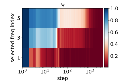
Figure 1: Using CG to learn $f(x)=\sin x+\sin 3x+\sin 5x$. $\Delta_{F}(k)$ of three selected important frequencies against different training epochs. Blue indicates large relative error, while red indicates small relative error.

We also use CG algorithm to train a convolutional network to fit MNIST. The F-Principle also holds in the training process, see Figure 2 for different variances $\delta$ of the Gaussian function.

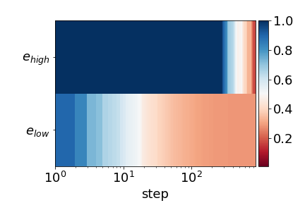
(a) $\delta=2$

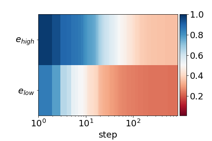
(b) $\delta=7$

Figure 2: Using CG to learn MNSIT. The F-Principle is examined for different $\delta$. $e_{\mathrm{low}}$ and $e_{\mathrm{high}}$ indicated by color against training epoch.

3.2 Truncated Newton algorithm

Truncated Newton algorithm (TNC), also called Newton Conjugate-Gradient, is a nonlinear method based on Newton method. The CG method is designed to solve positive definite systems, however, the Hessian matrix may have negative eigenvalues to lead to an inaccurate solution. TNC is a Hessian-free optimization method (Nash, 1985). The detail of TNC algorithm is given in Appendix.

In this experiment, we use TNC to train the 1-100-10-1 DNN to learn the target function with two frequency peaks, i.e., $f(x)=\sin x+\sin 3x$. Again, as shown in Figure 3, the DNN converges gradually from low-frequency to high frequency.

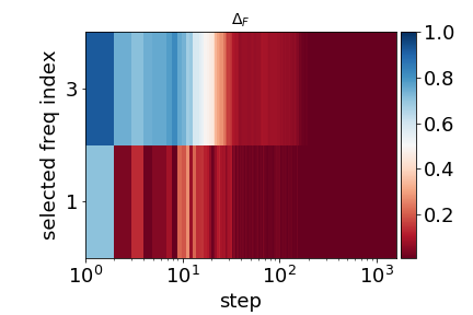
Figure 3: Using TNC to learn $f(x)=\sin x+\sin 3x$. $\Delta_{F}(k)$ of three selected important frequencies against different training epochs.

In our experiments, we point out that the results of training DNN by TNC to regress the target function (5) are not perfect, which is caused by the fact that the search direction is not the descent direction. This also may be influenced by the Hessian matrix, which may not keep positive definite in the training process. For $f(x)=\sin x+\sin 3x$, the low-frequency components is converged first, and it is regressed perfectly.

3.3 BFGS and L-BFGS

In this subsection, we use BFGS and L-BFGS, which are quasi-Newton methods, to train neural networks. The detail of BFGS algorithm is given in Appendix.

In Figure 4(a), we use BFGS to train a DNN of 1-100-10-1 to learn the target function (5). Similarly, the DNN converges gradually from low-frequency to high frequency.

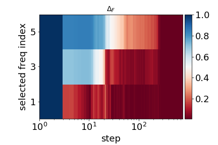
(a) BFGS

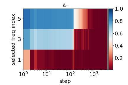
(b) L-BFGS

Figure 4: Using BFGS in (a) and L-BFGS in (b) to learn $f(x)=\sin x+\sin 3x+\sin 5x$. $\Delta_{F}(k)$ of three selected important frequencies against different training epochs.

L-BFGS uses a limited memory algorithm based on BFGS. This method only uses the data of the recent steps, which can simplify the computation and memory (Nocedal & Wright, 2006; Byrd et al., 1995). The detail of L-BFGS algorithm is given in Appendix.

In Figure 4(b), we use L-BFGS to train a DNN of 1-500-50-1 to learn the target function (5). It is clear that the DNN converges gradually from low-frequency to high frequency in this example.

We further use L-BFGS to train a CNN to learn MNIST. As shown in Fig. 5, for different filter width, we still observe that the high frequency part converges slower, that is, F-Principle.

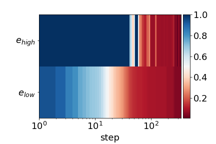
(a) $\delta=2$

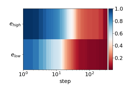
(b) $\delta=7$

Figure 5: Using L-BFGS to learn MNSIT. The F-Principle is examined for different $\delta$. $e_{\mathrm{low}}$ and $e_{\mathrm{high}}$ indicated by color against training epoch.

In this section, we have used experiments to show that a training algorithm, which uses gradient information but not a gradient-descent method, can still lead to the phenomenon of F-Principle. In the next section, we would show that even using a training algorithm without using gradient information, the F-Principle can still hold.

4 Gradient is not necessary

In this section, we use two non-gradient-based optimization algorithm (i.e., Powell’s method, Particle Swarm Optimization (PSO)) and a Monte-Carlo-like algorithm, to examine the F-Principle.

4.1 Powell’s method

Powell’s method, a conjugate direction method, performs sequential one-dimensional minimization along each vector of a direction set, in which the direction set is updated at each iteration (Powell, 1964). The method used here is a modification of Powell’s method. The loss function can be non-differentiable, since no derivative is taken. The detail of Powell’s method is given in Appendix.

The Powell’s method is slow in solving large scale optimization problems, such as training DNN, since it needs large internal memory and computations. Therefore, we use Powell’s method to train a small DNN of 1-100-1 to learn $f(x)=\sin x+\sin 3x$. Considering the two frequency peaks of the target function, as shown in Figure 6(a), one can see that the DNN converges the low-frequency components first.

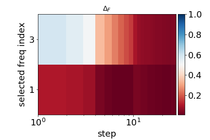
(a) Powell’s Method

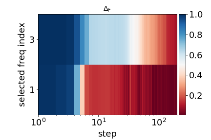
(b) PSO

Figure 6: Using non-gradient-based method to learn $f(x)=\sin x+\sin 3x$. $\Delta_{F}(k)$ of selected important frequencies against different training epochs.

4.2 Particle Swarm Optimization

Particle Swarm Optimization (PSO) does random search in parameter space, inspired by the moving of the swarm of birds. It can be viewed as a mid-level form of artificial life or biologically derived algorithm, and highly depends on stochastic processes. The PSO algorithm is given in appendix:

In this experiment, we use PSO to train a DNN of 1-100-10-1 to learn target function: $f(x)=\sin x+\sin 3x$. As shown in Figure 6(b), the DNN learns the low-frequency components first.

4.3 Monte-Carlo-Like algorithm

We found the F-Principle also holds in the following Monte-Carlo-Like algorithm: $\bm{\theta}_{j+1}$ is any element in

$$S=\{{\theta}|L(\theta)<L(\bm{\theta_{j}}),\left\|{\theta-\bm{\theta_{j}}}\right\|<\delta\},$$

unless $S$ is empty. We train a DNN of 1-500-200-1 to learn target function $f(x)=\sin x+\sin 3x$. Considering the important frequency peaks of the target function. As shown in Figure 7, the DNN converges the low-frequency components first.

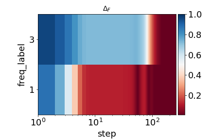
Figure 7: Using Monte-Carlo-Like algorithm to learn $f(x)=\sin x+\sin 3x$. $\Delta_{F}(k)$ of selected important frequencies against different training epochs.

5 Discussion and Conclusion

In this paper, we report the F-Principle in the training process of DNN using several non-gradient-descent-based methods. These empirical studies significantly extend the current understanding of the F-Principle. For future work, it is worth to study a mechanism of the F-Principle independent of gradient descent.

Appendix A Gradient

For the evaluation of gradient, we use the following difference scheme:

$$L_{\theta_{i}}(\bm{\theta}) \approx g_{\theta_{i}}(\bm{\theta})=\frac{L(\cdots,\bm{\theta_{i-1}},\bm{\theta_{i}}+\zeta,\bm{\theta_{i+1}},\cdots)-L(\cdots,\bm{\theta_{i-1}},\bm{\theta_{i}},\bm{\theta_{i+1}},\cdots)}{\zeta}$$ (6)

$$\nabla L =(L_{\theta_{1}},\cdots,L_{\theta_{i}},\cdots,L_{\theta_{P}})\approx g_{\theta}=(g_{\theta_{1}},\cdots,g_{\theta_{i}},\cdots,g_{\theta_{P}})\ \ \ \ \ \forall\ 0\leq i\leq P$$

Here, $P=(m_{0}+1)\times m_{1}+(m_{1}+1)\times m_{2}+(m_{2}+1)\times m_{3}+\cdots(m_{H-1}+1)\times m_{H}$ is the number of the parameters, and $\zeta$ is a small number defined by user, usually associated with $\epsilon$ or the accuracy of the machine’s floating point: $acc$. We set $\zeta=\sqrt{acc}$, which is approximately $1.49\times 10^{-8}$ in the following experiments.

Appendix B 1-d search

Before the introduction of the 1-d line search, there are some sub-options needed to introduce first, the evaluation of $\alpha_{0}$ is in the Algorithm 1:

Algorithm 1 Evaluation of $\alpha_{0}$ in 1-d search

1:procedure  (Input $\alpha_{\min}$, $\alpha_{\max}$, $\alpha_{r}$, $\phi$, $i$)

2:     if $i>0$ then

3:         $cchk:=0.2\left|\alpha_{\max}-\alpha_{\min}\right|,\alpha_{0}:=cubicmin(\alpha_{\max},\alpha_{\min},\alpha_{r},\phi)$      

4:     if $i>0$ or $min\{\left|\alpha_{\max}-\alpha_{0}\right|,\left|\alpha_{\min}-\alpha_{0}\right|\}\leq cchk$ then

5:         $qchk:=0.1\left|\alpha_{\max}-\alpha_{\min}\right|,\ \alpha_{0}:=\min(\alpha_{\max},\alpha_{\min},\phi)$

6:     else

7:         output $\alpha_{0}$ and end this algorithm      

8:     if $\min\{\left|\alpha_{\max}-\alpha_{0}\right|,\left|\alpha_{\min}-\alpha_{0}\right|\}\leq qchk$ then

9:         $\alpha_{0}:=\frac{\alpha_{\max}+\alpha_{\min}}{2}$, output $\alpha_{0}$ and end this algorithm      

In the algorithm, $cubicmin(\alpha_{\max},\alpha_{\min},\alpha_{r},\phi)$ returns the minimum of $C(x)$ in $[\alpha_{\min},\alpha_{\max}]$, where $C(x)$ is a cubic polynomial that goes through the points $(\alpha_{\min},\phi(\alpha_{\min}))$, $(\alpha_{\max},\phi(\alpha_{\max})),\ (\alpha_{r},\phi(\alpha_{r}))$ with derivative at $\alpha_{\min}$ of $\phi^{\prime}(\alpha_{\min})$; in the Step3, $quadmin(\alpha_{\max},\alpha_{\min},\phi)$ returns the minimum of $Q(x)$ in $[\alpha_{\min},\alpha_{\max}]$, where $Q(x)$ is a quadratic polynomial that goes through the points $(\alpha_{\min},\phi(\alpha_{\min}))$, $(\alpha_{\max},\phi(\alpha_{\max}))$ with derivative at $\alpha_{\min}$ of $\phi^{\prime}(\alpha_{\min})$.

In the 1-d line search, under a given boundary $\alpha_{\max}$, we use the following method (for the computation of $\bm{\theta_{k+1}}$ in our algorithms) to find a point in interval $[\bm{\theta_{k}},\bm{\theta_{k}}+\alpha_{\max}\bm{d}]$, which makes the searching process dsatisfy strong Wolfe conditions in Algorithm 2.

Algorithm 2 Finding $\alpha_{0}$ satisfy strong Wolfe conditions

1:procedure  (Input Input $\bm{\theta_{k}}$, direction $\bm{d}$)

2:     Set $i:=0$, $\alpha_{min}:=0$, $\alpha_{max}:=50$, $\alpha_{0}=1$, $\alpha_{r}=0$, $\sigma=0.9$, $\rho=10^{-4}$, $maxiter=10$, $\phi(\alpha)=L(\bm{\theta_{k}}+\alpha\bm{d})$, $\alpha_{0}=1.01\times 2\frac{\phi(\alpha_{0})-\phi(0)}{\phi^{\prime}(0)}$

3:     if $\alpha_{0}<0$ or $\alpha_{0}=Null$ then

4:         $\alpha_{0}=1$      

5:     while $i\leq maxiter$ and $\left|\phi^{\prime}(\alpha_{0})\right|>-\sigma\phi^{\prime}(\alpha_{min})$ do

6:         if $\phi(\alpha_{0})>\phi(0)+\rho\alpha_{0}\phi^{\prime}(0)$ or $\phi(\alpha_{0})\geq\phi(\alpha_{min})$ then

7:              $\alpha_{r}:=\alpha_{max}$, $\alpha_{max}:=\alpha_{0}$;

8:         else if $\phi^{\prime}(\alpha_{0})(\alpha_{max}-\alpha_{min})\geq 0$ then

9:              $\alpha_{r}:=\alpha_{max}$, $\alpha_{max}:=\alpha_{min}$;

10:              $\alpha_{min}=\alpha_{0}$;

11:         else

12:              $\alpha_{r}=\alpha_{min}$;

13:              $\alpha_{min}=\alpha_{0}$;          

14:         Evaluate $\alpha_{0}$ using $\alpha_{min}$, $\alpha_{max}$, $\alpha_{r}$, $i$, $\phi$;

15:         $i:=i+1$      

16:     if $\left|\phi^{\prime}(\alpha_{0})\right|\leq-\sigma\phi^{\prime}(\alpha_{min})$ then

17:         Output: $\bm{\theta_{k+1}}:=\bm{\theta_{k}}+\alpha_{0}\bm{d}$, and end this algorithm;

18:     else

19:         Output: ’algorithm failed’ and end this algorithm;      

In algorithm 2, there is an option called ${}^{\prime}Evaluate\ \alpha_{0}\ ^{\prime}$, which is the algorithm 1, and $\phi^{\prime}$ is defined by the difference scheme similar in Appendix A. One may use some other algorithm to make the searching satisfy strong Wolfe conditions, the above one is also used in Python’s scipy.optimize.

Algorithm 3 CG

1:procedure  (Input $\bm{\theta_{j}}:=\theta_{0}$, $\epsilon>0$, $M\in\mathbb{N}$)

2:     Set $j:=0$;

3:     Compute $g_{j}=g(\bm{\theta_{j}})$;

4:     while $j\leq M$ and $\left\|{g_{j}}\right\|>\epsilon$ do

5:         $\bm{d_{j}}:=-g_{j}$;

6:         Do 1-d line search $(\bm{d}:=\bm{d_{j}})$, evaluate $\bm{\theta_{j+1}}$, $j:=j+1$;

7:         Compute $g_{j}=g(\bm{\theta_{j}})$;

8:         $\beta:=\frac{g_{j}^{T}(g_{j}-g_{j-1})}{g_{j-1}^{T}g_{j-1}}$, $\bm{d_{j}}:=-g_{j}+\beta d_{j-1}$;

9:         if $\bm{d_{j}}^{T}g_{j}>0$ then

10:              $\bm{d_{j}}:=-g_{j}$;               

11:     output $\bm{\theta_{j}}$ and end this algorithm;

Algorithm 4 TNC

1:procedure  (Input $\bm{\theta_{j}}:=\theta_{0}$, $\epsilon>0$, $M\in\mathbb{N}$)

2:     Set $j:=0$;

3:     Compute $g_{j}=g(\bm{\theta_{j}})$, $H_{j}=H(\bm{\theta_{j}})$;

4:     while $j\leq M$ and $\left\|{g_{j}}\right\|>\epsilon$ do

5:         $p_{0}=0$, $r_{0}=-g_{j}$, $l_{0}=r_{0}$, $\delta_{0}=r_{0}^{T}r_{0}$, $i=0$;

6:         while $l_{i}^{T}q_{i}>\epsilon\delta_{i}$ and $i<M$ do

7:              $\alpha_{i}=\frac{r_{i}^{T}r_{i}}{l_{i}^{T}q_{i}}$, $p_{i+1}=p_{i}+\alpha_{i}l_{i}$, $r_{i+1}=r_{i}-\alpha_{i}q_{i}$

8:              if $\frac{\left\|{r_{i+1}}\right\|}{\left\|{g_{j}}\right\|}\leq\eta$ then

9:                  $\bm{d_{j}}=\bm{p_{i}}$;

10:                  break;

11:              else

12:                  $\beta_{i}=\frac{r_{i+1}^{T}r_{i+1}}{r_{i}^{T}r_{i}}$, $l_{i+1}=r_{i+1}+\beta_{i}l_{i}$, $\delta_{i+1}=r_{i+1}^{T}r_{i+1}+\beta_{i}^{2}\delta_{i}$; $i:=i+1$;                        

13:         $\bm{d_{j}}=\left\{\begin{aligned} l_{0}&\ i=0\\ p_{i}&\ i\geq 0\end{aligned}\right.$

14:         Do 1-d line search $(\bm{d}:=\bm{d_{j}})$, evaluate $\bm{\theta_{j+1}}$, $j:=j+1$;

15:         Compute $g_{j}=g(\bm{\theta_{j}})$, $H_{j}=H(\bm{\theta_{j}})$;      

16:     output $\bm{\theta_{j}}$ and end this algorithm;

Algorithm 5 BFGS

1:procedure  (Input $\bm{\theta_{j}}:=\theta_{0}$, $\epsilon>0$, $M\in\mathbb{N}$, $H_{0}=I$)

2:     Set $j:=0$;

3:     Compute $g_{j}=g(\bm{\theta_{j}})$;

4:     while $j\leq M$ and $\left\|{g_{j}}\right\|>\epsilon$ do

5:         $\bm{d_{j}}:=-H_{j}g_{j}$;

6:         Do 1-d line search $(\bm{d}:=\bm{d_{j}})$, evaluate $\bm{\theta_{j+1}}$, $g_{j+1}=g(\bm{\theta_{j+1}})$, $s_{j}=\bm{\theta_{j+1}}-\bm{\theta_{j}}$, $y_{j}=g_{j+1}-g_{j}$;

7:         Compute $H_{j+1}=(I-\frac{s_{j}y_{j}^{T}}{s_{j}^{T}y_{j}})H_{j}(I-\frac{y_{j}s_{j}^{T}}{s_{j}^{T}y_{j}})+\frac{s_{j}s_{j}^{T}}{s_{j}^{T}y_{j}}$;

8:         $\beta:=\frac{g_{j}^{T}(g_{j}-g_{j-1})}{g_{j-1}^{T}g_{j-1}}$, $\bm{d_{j}}:=-g_{j}+\beta d_{j-1}$, $j=j+1$;      

9:     output $\bm{\theta_{j}}$ and end this algorithm;

Algorithm 6 L-BFGS

1:procedure  (Input $\bm{\theta_{j}}:=\theta_{0}$, $\epsilon>0$, $M\in\mathbb{N}$, $m\in\mathbb{N}$)

2:     Set $j:=0$;

3:     Compute $g_{j}=g(\bm{\theta_{j}})$, $\bm{d_{0}}=g_{0}$;

4:     while $j\leq M$ and $\left\|{g_{j}}\right\|>\epsilon$ do

5:         Do 1-d line search $(\bm{d}:=\bm{d_{j}})$, evaluate $\bm{\theta_{j+1}}$, $g_{j+1}=g(\bm{\theta_{j+1}})$, $s_{j}=\bm{\theta_{j+1}}-\bm{\theta_{j}}$, $y_{j}=g_{j+1}-g_{j}$, $\rho_{j}=\frac{1}{y_{j}^{T}s_{j}}$, $j:=j+1$;

6:         if $j\leq m$ then

7:              $\delta:=0$, $L:=j$;

8:         else

9:              $\delta:=j-m$, $L=m$;          

10:         $q_{L}=g_{j}$, $i=L-1$;

11:         while $i\geq 0$ do

12:              $k=i+\delta$, $\alpha_{i}=\rho_{k}s_{k}^{T}q_{i+1}$, $q_{i}=q_{i+1}-\alpha_{i}y_{k}$;

13:              $i:=i-1$;          

14:         $r_{0}=Iq_{0}=q_{0}$, $i:=0$;

15:         while $i\leq L-1$ do

16:              $k=i+\delta$, $\beta_{i}=\rho_{k}y_{k}^{T}r_{i}$, $r_{i+1}=r_{i}+(\alpha_{i}-\beta_{i})s_{k}$;

17:              $i:=i+1$;          

18:         $\bm{d_{j}}=r_{L}$;      

19:     output $\bm{\theta_{j}}$ and end this algorithm;

Algorithm 7 Powell’s algorithm

1:procedure  (Input $\bm{\theta_{j}}:=\theta_{0}$, $y_{0}=\bm{\theta_{j}}$, $\epsilon>0$, $M\in\mathbb{N}$, $S_{0}=(s_{0},s_{1},\cdots,s_{p-1})=I$)

2:     Set $j:=0$, $k:=1$;

3:     Compute $g_{j}=g(\bm{\theta_{j}})$;

4:     while $k\leq p$ do

5:         $\lambda_{k-1}=argminL(y_{k-1}+\lambda s_{k-1})$, $y_{k}=y_{k-1}+\lambda_{k-1}s_{k-1}$;

6:         $k:=k+1$;      

7:     $s_{p}=y_{p}-y_{0}$;

8:     while $j\leq M$ and $\left\|{s_{p}}\right\|>\epsilon$ do

9:         $\Delta_{m}=max\{L(y_{i})-L(y_{i+1})$, $0\leq i\leq p-1\}=L(y_{m})-L(y_{m+1})$;

10:         $f_{1}=L(y_{0})$, $f_{2}=L(y_{p})$, $f_{3}=L(2y_{p}-y_{0})$;

11:         if $2(f_{1}-2f_{2}+f_{3})(f_{1}-f_{2}-\Delta_{m})^{2}<\Delta(f_{1}-f_{3})^{2}$ then

12:              $\lambda_{p}=argminL(y_{p}+\lambda s_{p})$, $\bm{\theta_{j+1}}=y_{p}+\lambda_{p}s_{p}$;

13:              $s_{k}=s_{k+1}$, for $k=m:p-1$;

14:         else

15:              $\bm{\theta_{j+1}}=y_{p}$, $j:=j+1$;          

16:         while $k\leq p$ do

17:              $\lambda_{k-1}=argminL(y_{k-1}+\lambda s_{k-1})$, $y_{k}=y_{k-1}+\lambda_{k-1}s_{k-1}$;

18:              $k:=k+1$;          

19:         $s_{p}=y_{p}-y_{0}$;      

20:     output $\bm{\theta_{j}}$ and end this algorithm; Note: This algorithm uses golden section method (0.618 method) to find the minimum of $\lambda$ in the bracket between $[0,1]$.

Algorithm 8 PSO

1:procedure  (Input $\bm{\theta_{j}}:=\theta_{0}$, $\epsilon>0$, $M\in\mathbb{N}$, $m\in\mathbb{N}$, $N=2p$, $H_{0}=(I,-I)=(h_{1},\cdots,h_{N})$, $\bm{\theta_{j}}^{(1)},\bm{\theta_{j}}^{(2)},\cdots,\bm{\theta_{j}}^{(N)}$ are randomly set around $\theta_{0}$)

2:     Set $j:=0$;

3:     Set ${\alpha_{j}}^{(i)}=\arg\min\{L(\alpha),\alpha\in\{L(\bm{\theta_{0}}^{(i)}),L(\bm{\theta_{1}}^{(i)}),\cdots,L(\bm{\theta_{j}}^{(i)})\}\},\ \forall 1\leq i\leq N$

4:     $\bm{\theta_{j+1}}=\arg\min\{L(\alpha),\alpha\in\{{\alpha_{j}}^{(1)},{\alpha_{j}}^{(2)},\cdots,{\alpha_{j}}^{(N)}\}\}$;

5:     while $j\leq M$ and $\left\|{\bm{\theta_{j-m}}-\bm{\theta_{j}}}\right\|>\epsilon$ do

6:         $\bm{\theta_{j}}^{(i)}:=\bm{\theta_{j-1}}^{(i)}+h_{i}+2r_{1}^{(i,j)}({\alpha^{(i)}_{j}}-\bm{\theta_{j-1}}^{(i)})+2r_{2}^{(i,j)}(\bm{\theta_{j}}-\bm{\theta_{j-1}}^{(i)})$;

7:         Set ${\alpha_{j}}^{(i)}=\arg\min\{L(\alpha),\alpha\in\{L(\bm{\theta_{0}}^{(i)}),L(\bm{\theta_{1}}^{(i)}),\cdots,L(\bm{\theta_{j}}^{(i)})\}\},\ \forall 1\leq i\leq N$

8:         $\bm{\theta_{j+1}}=\arg\min\{L(\alpha),\alpha\in\{{\alpha_{j}}^{(1)},{\alpha_{j}}^{(2)},\cdots,{\alpha_{j}}^{(N)}\}\}$;

9:         $j:=j+1$;      

10:     output $\bm{\theta_{j}}$ and end this algorithm; Note: $r_{1}^{(i,j)},\ r_{2}^{(i,j)}\sim U([0,1])$, while $U([0,1])$ is the uniform distribution on $[0,1]$.

Algorithm 9 Monte-Carlo-like method

1:procedure  (Input $\bm{\theta_{j}}:=\theta_{0}$, $\epsilon>0$, $M\in\mathbb{N}$, $m\in\mathbb{N}$)

2:     Set $j:=0$;

3:     while $j\leq M$ and $\left\|{L(\bm{\theta}_{j})-L(\bm{\theta}_{j-m})}\right\|>\epsilon$ do

4:         $\bm{\theta^{(k)}_{j}}\sim N(\bm{\theta_{j}},\delta)$ independently, $\forall\ 1\leq k\leq M$;

5:         $\bm{\theta_{j+1}}:=argmin\{L(\bm{\theta_{j}}),L(\bm{\theta_{j}^{(k)}})|\ \forall\ 1\leq k\leq M\}$, $j:=j+1$      

6:     output $\bm{\theta_{j}}$ and end this algorithm;

References

• BAAI (2020) BAAI. Suggested notation for machine learning. https://github.com/Mayuyu/suggested-notation-for-machine-learning, 2020.
• Biland et al. (2019) Simon Biland, Vinicius C Azevedo, Byungsoo Kim, and Barbara Solenthaler. Frequency-aware reconstruction of fluid simulations with generative networks. arXiv preprint arXiv:1912.08776, 2019.
• Bordelon et al. (2020) Blake Bordelon, Abdulkadir Canatar, and Cengiz Pehlevan. Spectrum dependent learning curves in kernel regression and wide neural networks. arXiv preprint arXiv:2002.02561, 2020.
• Byrd et al. (1995) R H Byrd, P Lu, and J. Nocedal. A limited memory algorithm for bound constrained optimization. SIAM Journal on Scientific and Statistical Computing, 16(5):1190–1208, 1995.
• Cai et al. (2019) Wei Cai, Xiaoguang Li, and Lizuo Liu. A phase shift deep neural network for high frequency wave equations in inhomogeneous media. Arxiv preprint, arXiv:1909.11759, 2019.
• Cao et al. (2019) Yuan Cao, Zhiying Fang, Yue Wu, Ding-Xuan Zhou, and Quanquan Gu. Towards understanding the spectral bias of deep learning. arXiv preprint arXiv:1912.01198, 2019.
• E et al. (2019) Weinan E, Chao Ma, and Lei Wu. Machine learning from a continuous viewpoint. arXiv preprint arXiv:1912.12777, 2019.
• Jacot et al. (2018) Arthur Jacot, Franck Gabriel, and Clément Hongler. Neural tangent kernel: Convergence and generalization in neural networks. In Advances in neural information processing systems, pp. 8571–8580, 2018.
• Jagtap et al. (2020) Ameya D Jagtap, Kenji Kawaguchi, and George Em Karniadakis. Adaptive activation functions accelerate convergence in deep and physics-informed neural networks. Journal of Computational Physics, 404:109136, 2020.
• Li et al. (2020) Xi-An Li, Zhi-Qin John Xu, and Lei Zhang. A multi-scale dnn algorithm for nonlinear elliptic equations with multiple scales. Communications in Computational Physics, 28(5):1886–1906, 2020.
• Liu et al. (2020) Ziqi Liu, Wei Cai, and Zhi-Qin John Xu. Multi-scale deep neural network (mscalednn) for solving poisson-boltzmann equation in complex domains. Communications in Computational Physics, 28(5):1970–2001, 2020.
• Luo et al. (2019) Tao Luo, Zheng Ma, Zhi-Qin John Xu, and Yaoyu Zhang. Theory of the frequency principle for general deep neural networks. arXiv preprint arXiv:1906.09235, 2019.
• Luo et al. (2020a) Tao Luo, Zheng Ma, Zhiwei Wang, Zhi-Qin John Xu, and Yaoyu Zhang. Fourier-domain variational formulation and its well-posedness for supervised learning. arXiv preprint arXiv:2012.03238, 2020a.
• Luo et al. (2020b) Tao Luo, Zheng Ma, Zhi-Qin John Xu, and Yaoyu Zhang. On the exact computation of linear frequency principle dynamics and its generalization. arXiv preprint arXiv:2010.08153, 2020b.
• Ma et al. (2020) Chao Ma, Lei Wu, and E Weinan. The slow deterioration of the generalization error of the random feature model. In Mathematical and Scientific Machine Learning, pp. 373–389. PMLR, 2020.
• Nash (1985) Stephen G Nash. Preconditioning of truncated-newton methods. SIAM Journal on Scientific and Statistical Computing, 6(3):599–616, 1985.
• Nocedal & Wright (2006) Jorge Nocedal and Stephen Wright. Numerical optimization. Springer Science & Business Media, 2006.
• Powell (1964) Michael JD Powell. An efficient method for finding the minimum of a function of several variables without calculating derivatives. The computer journal, 7(2):155–162, 1964.
• Rahaman et al. (2019) Nasim Rahaman, Devansh Arpit, Aristide Baratin, Felix Draxler, Min Lin, Fred A Hamprecht, Yoshua Bengio, and Aaron Courville. On the spectral bias of deep neural networks. International Conference on Machine Learning, 2019.
• Ronen et al. (2019) Basri Ronen, David Jacobs, Yoni Kasten, and Shira Kritchman. The convergence rate of neural networks for learned functions of different frequencies. In Advances in Neural Information Processing Systems, pp. 4763–4772, 2019.
• Wang et al. (2020a) Feng Wang, Alberto Eljarrat, Johannes Müller, Trond R Henninen, Rolf Erni, and Christoph T Koch. Multi-resolution convolutional neural networks for inverse problems. Scientific reports, 10(1):1–11, 2020a.
• Wang et al. (2020b) Jihong Wang, Zhi-Qin John Xu, Jiwei Zhang, and Yaoyu Zhang. Implicit bias with ritz-galerkin method in understanding deep learning for solving pdes. arXiv preprint arXiv:2002.07989, 2020b.
• Xu et al. (2019a) Zhi-Qin J Xu, Yaoyu Zhang, and Yanyang Xiao. Training behavior of deep neural network in frequency domain. International Conference on Neural Information Processing, pp.  264–274, 2019a.
• Xu & Zhou (2020) Zhi-Qin John Xu and Hanxu Zhou. Deep frequency principle towards understanding why deeper learning is faster. arXiv preprint arXiv:2007.14313, AAAI-21, 2020.
• Xu et al. (2019b) Zhi-Qin John Xu, Yaoyu Zhang, Tao Luo, Yanyang Xiao, and Zheng Ma. Frequency principle: Fourier analysis sheds light on deep neural networks. arXiv preprint arXiv:1901.06523, 2019b.
• Yang & Salman (2019) Greg Yang and Hadi Salman. A fine-grained spectral perspective on neural networks. arXiv preprint arXiv:1907.10599, 2019.
• You et al. (2020) Haoran You, Chaojian Li, Pengfei Xu, Yonggan Fu, Yue Wang, Xiaohan Chen, Yingyan Lin, Zhangyang Wang, and Richard G Baraniuk. Drawing early-bird tickets: Towards more efficient training of deep networks. International Conference on Learning Representations, 2020.
• Zhang et al. (2019) Yaoyu Zhang, Zhi-Qin John Xu, Tao Luo, and Zheng Ma. Explicitizing an implicit bias of the frequency principle in two-layer neural networks. arXiv preprint arXiv:1905.10264, 2019.