Meta Variationally Intrinsic Motivated Reinforcement Learning for Decentralized Traffic Signal Control

Abstract

The goal of traffic signal control is to coordinate multiple traffic signals to improve the traffic efficiency of a district or a city. In this work, we propose a novel Meta Variationally Intrinsic Motivated (MetaVIM) RL method, and aim to learn the decentralized polices of each traffic signal only conditioned on its local observation. MetaVIM makes three novel contributions. Firstly, to make the model available to new unseen target scenarios, we formulate the traffic signal control as a meta-learning problem over a set of related tasks. The train scenario is divided as multiple partially observable Markov decision process (POMDP) tasks, and each task corresponds to a traffic light. In each task, the neighbours are regarded as an unobserved part of the state. Secondly, we assume that the reward, transition and policy functions vary across different tasks but share a common structure, and a learned latent variable conditioned on the past trajectories is proposed for each task to represent the specific information of the current task in these functions, then is further brought into policy for automatically trade off between exploration and exploitation to induce the RL agent to choose the reasonable action. In addition, to make the policy learning stable, four decoders are introduced to predict the received observations and rewards of the current agent with/without neighbour agents’ policies, and a novel intrinsic reward is designed to encourage the received observation and reward invariant to the neighbour agents. Empirically, extensive experiments conducted on CityFlow demonstrate that the proposed method substantially outperforms existing methods and shows superior generalizability.

Introduction

Traffic signals that direct traffic movements play an important role for efficient transportation. Conventional methods control traffic signals by fixed-time plans (?) or hand-crafted heuristics (?). However, these methods are predefined and cannot adapt to dynamic and uncertain traffic conditions. Recently, deep reinforcement learning (RL) (?; ?; ?; ?; ?) has been applied to traffic signal control, where an RL agent directly interacts with the environment and learns to control an intersection. RL methods have demonstrated superior performance to conventional control methods. However, most of existing RL methods consider an intersection independently, ignoring the interaction between neighboring agents (intersections), and thus obtain only suboptimal performance. Ideally, optimizing traffic signal control in a road network can be modelled as a multi-agent reinforcement learning (MARL) problem and learned by centralized learning (?; ?; ?). However, as the joint action space grows exponentially with the number of agents, it is infeasible to learn in a large road network. In addition, centralized learning needs agents’ communication or the joint state, which are often unavailable or costly in realistic deployment. Therefore, how to learn decentralized policies in the MARL setting is the key to advance RL for traffic signal control.

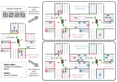
Figure 1: Illustration of the task uncertainty in multi-intersection control scenario. For intersection 1, the current policy is to choose North-South-Straight-Green conditioned on its local observation. However, under the same state, take the same action, when neighbour’s policy changes, transition to different states.

To learn effective decentralized policies, there are two main challenges. Firstly, in a city or a district, there are thousands of intersections. It is impractical to learn an individual policy for each intersection. Parameter sharing may help. However, each intersection has different traffic pattern, and a simply shared policy hardly learns and acts optimally at all the intersections. To address this challenge, we formulate traffic signal control in a road network as a meta-learning problem; i.e., traffic signal control at each intersection is a task and a policy is learned to adapt to various tasks. Reward function and state transition of these tasks vary across these tasks but also share similarity, since they follow the same traffic rules and have similar optimization goals. Therefore, we represent each task as a learned and low-dimensional latent variable, which is obtained by encoding the past trajectory in each task. The latent variable is a part of the input of the learned policy, which captures task specific information and help to improve the policy adaption.

Secondly, for each task, the received rewards and observations are uncertain to the current agent as illustrated in Fig. 1, which may lead the policy learning unstable and non-convergent. In other words, even if the agent performs the same action on a same observation at different times, the agent may receive different rewards and next observations because neighbour agents may perform different actions. To overcome this, four decoders are introduced to predict the next observations and rewards with/without neighbour agents’ policies, respectively. The decoders also take as input the latent variable to identify specific tasks. In order to make the learning stable, we argue that the prediction of observation and reward should be robust to neighbour agents’ policies. Hence, an intrinsic reward is designed to encourage the policy to reduce the differences between the predicted reward (and observation) only relying on the current agent’s policy and the one using both the current agent’s and the neighbour agents’ policies.

Traffic signal control is also modeled as a meta-learning problem in (?). However, our method is advanced in several ways: firstly, their meta-training is based on multiple independent MDPs and ignore the influence of neighbour agents, while our method takes neighbour agents’ policies into consideration that is critical in learning decentralized policies; secondly, our method learns a latent variable to represent task specific information, which can not only balance exploration and exploitation (?), but also help to learn the shared structures of reward and transition across tasks.

Empirically, we conduct extensive experiments on CityFlow (?) in Hangzhou (China), Jinan (China), New York (USA), and Shenzhen (China) road networks under various traffic patterns and demonstrate that the proposed method substantially outperforms existing methods and shows superior adaptivity.

Related Work

Reinforcement Learning in Traffic Signal Control

Most RL based traffic signal control methods formulates the task as a single agent learning problem or decentralized learning problem of multi-agent such as (?; ?; ?; ?; ?; ?; ?). All these above methods aim to learn the policy by the observation only and ignore the influence of neighbours. Several methods (?; ?) consider the neighbours, while they both need the whole state in testing and are hard to deploy in the unseen target scenarios. To improve the generality of the model, (?) employs mete-learning to the task. Compared with (?), our method learns a latent variable to help to learn the task-shared structure of policy, and uses neighbour’s information to form intrinsic motivation.

Multi-agent Reinforcement Learning

Independent learning (IL) (?) suffers from the environmental non-stationarity owing to other agents keeping updating. Centralized learning (CL) treats the entire multi-agent environment as a joint single-agent environment. Many current state-of-the-art methods follow Centralized training and decentralized execution (CTDE) paradigm. For instance, COMA  (?) and MADDPG (?) explore multi-agent policy gradients for the settings of local reward and shared reward respectively. Meanwhile, value-function factorization is the most popular method for value-based multi-agent RL. VDN (?), QMIX (?) and QTRAN (?) are proposed to directly factorize the joint action-value function into individual ones for decentralized execution.

Latent Variable and Meta-Learning

Recently, a series of meta-learning methods have been proposed combined with latent variable. (?) use priviledged information separately learns the policy and the task belief. (?) disentangles task inference and control by using online probabilistic filtering of latent task variables to solve a new task from small amounts of experience. (?) recast memory-based meta-learning within a Bayesian framework. Model parameters is patitioned into context parameters and shared parameters in (?), and the shared parameters are meta-trained and shared across tasks. MDP parameters are obtained from the context using generalized linear models in (?).

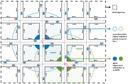
Figure 2: The illustration of POMDPs in traffic signal control. We formulate the traffic signal control as a meta-learning problem across multiple POMDPs. In a POMDP, agent can only obtain its local observation and regard the neighbours’ policies as the unobserved part of the environment.

Intrinsic Reward

Intrinsic reward is usually motivated to perform an activity for its own sake and personal rewards. In (?), curiosity is regarded as the intrinsic reward signal. (?) uses the form of $\alpha/\sqrt{N}$ as the intrinsic reward.(?) uses density models to measure an agent’s uncertainty about its environment. (?) uses asymmetric self-play as intrinsic reward. (?) uses the errors between cooperating and performing actions sequentially as an intrinsic reward. (?) uses the KL divergence between the action distributions of neighbors knowing my actions and ignorant of my actions.

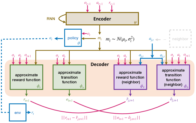
Figure 3: MetaVIM consists of a mVAE and a policy network. RL agent is augmented with a latent variable $m_{i}$, obtained by encoding over past trajectories $\tau_{i,:t}$ of POMDP$(i)$ to represent the POMDP-specific information. The traffic signal control is formulated as a meta-learning problem over a set of POMDPs, the multi-head decoder $\bm{d_{i}(\cdot)}$ is trained over a larger and diverse replay buffer for capturing the common knowledge across tasks. Intrinsic reward is the inference error to encourage the approximations invariant to the neighbours.

Problem Statement

The method aims to learn the traffic signal control policy from the training transportation scenario, and the learned policy can be generalized to the unseen scenarios except the training scenario. Therefore, the meta-learning framework is employed. Specifically, the training scenario is divided into multiple Partially Observable Markov Decision Processes (POMDPs) (?), and POMDP$(i)$ corresponds to the traffic signal $i$ where $i\in{0,1,...,N}$ and $N$ is the number of traffic signals (or intersections) in the scenario. For each traffic signal $i$, POMDP$(i)$ is defined by the tuple $\langle\mathcal{O}_{i},\mathcal{S}_{i},\mathcal{A}_{i},{R}_{i},{T}_{i},H_{i}\rangle$ consisting of: $\mathcal{O}_{i}$ is a set of local observations which can be visited by each agent, $\mathcal{S}_{i}$ is a finite set of resulting states, $\mathcal{A}_{i}$ is a finite set of actions, $\mathcal{R}_{i}$ is the reward function, $\mathcal{T}_{i}$ is the transition function, $H_{i}$ is the horizon (episode length). Observation $o_{i}\in\mathcal{O}_{i}$ includes the number of vehicles on each incoming lanes $x(m)\left(m\in L_{in}\right)$ and the current phase of the intersection, where phase is the part of the signal cycle allocated to any combination of traffic movements receiving the right-of-way simultaneously during one or more intervals (?). A four-phase diagram includes North-South-Straight-Green, North-South-Left-Green, East-West-Straight-Green and East-West-Straight-Green respectively, as illustrated in Fig. 1. Action space $\mathcal{A}_{i}$ is the finite discrete set of possible actions where each action means one phase is selected. At the time step $t$, the agent chooses action $a_{i,t}\in\mathcal{A}_{i}$. We assume the different traffic signals have the same action space as same as (?; ?). State $s_{i,t}\in\mathcal{S}_{i}$ is the POMDP state at time step $t$ including the observed part $o_{i,t}$ and the unobserved part $u_{i,t}=\{{o}_{i,t}^{-1},{a}_{t}^{-1}\}$, where ${o}_{i,t}^{-1}$ and ${a}_{i,t}^{-1}$ is the observations and actions of the neighbours, respectively. The neighbours are modeled as a part of the environment to the current traffic signal, and this is also the main difference compared with the existing work (?) which ignores the influence of the neighbours. Transition function ${T}_{i}(o_{i,t+1},u_{i,t+1}|o_{i,t},a_{i,t},u_{i,t})$ is a transition probability function induced by performing action $a_{i,t}$ on the POMDP$i$ where $t$ is the time clamp. At the time step $t+1$, $o_{i,t+1}$ and $u_{i,t+1}$ are independent with each other, hence ${T}_{i}(o_{i,t+1},u_{i,t+1}|o_{i,t},a_{i,t},u_{i,t})={T}_{i}(o_{i,t+1}|o_{i,t},a_{i,t},u_{i,t})\times{T}_{i}(u_{i,t+1}|o_{i,t},a_{i,t},u_{i,t})$. Reward function $r_{i,t}=R_{i}(o_{i,t+1},u_{i,t+1},o_{i,t},u_{i,t},a_{t})$ is the payoff of performing the action $a_{t}$ in current state.

In a POMDP, the transition and reward functions are unknown, while the results $o_{(i,t+1)}$ is observed in both training and testing, and $r_{i,t}$ is observed in training at time $t+1$. Based on the observations, the parameterized policy function of current POMDP is defined as the probability of choosing each action $\pi^{\theta}_{i}(a_{i,t}|o_{i,t})$, where $a_{i,t}\in\mathcal{A}$ and $\theta$ is the network parameter. In the typical meta-learning setting, the reward, transition and policy functions that are unique to each POMDP are unknown, but also share some structure across the different POMDPs (?). Therefore, a learned stochastic latent variable $m_{i}$ is proposed to represent each POMDP$(i)$. Then the reward, transition and policy functions for each POMDP$(i)$ can be approximated as follows:

$$\pi^{\theta}_{i}(a_{i,t}|o_{i,t})\approx\pi^{\theta}(a_{i,t}|o_{i,t};m_{i}),$$

$$R_{i}(o_{i,t+1},u_{i,t+1},o_{i,t},u_{i,t},a_{t})$$

$$\ \ \ \approx R(o_{i,t+1},u_{i,t+1},o_{i,t},u_{i,t},a_{t};m_{i}),$$

$$T_{i}(o_{i,t+1},u_{i,t+1}|o_{i,t},a_{i,t},u_{i,t})$$

$$\ \ \ \approx T(o_{i,t+1},u_{i,t+1}|o_{i,t},a_{i,t},u_{i,t};m_{i}),$$ (1)

where $\pi^{\theta}$, $R$ and $T$ are shared across different POMDPs. Since $m_{i}$ is sufficient to identify POMDP$(i)$, we remove the subscript $i$ of $a_{i,t}$, $o_{i,t}$ and $u_{i,t}$ hereafter for simplicity. In summary, the goal of the method is how to infer the POMDP-specific latent variable $m_{i}$ and learn the POMDP-shared $\pi^{\theta}_{i}$ by meta-learning.

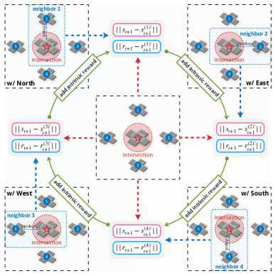
Figure 4: Intrinsic reward illustration. Intrinsic motivation is considered as the sum of the predicted error between the inferences with/without neighbor’s policy under four circumstances (for 4-way intersection).

Method

Model

As illustrated in Fig. 3, the framework of the proposed Meta Variationally Intrinsic Motivated (MetaVIM) model consists of 2 main parts: Firstly, a multi-head VAE (mVAE) contains a encoder and four decoders where the encoder employs the past observation, action and reward trajectory $\tau_{i,:t}$ to generate the latent variables $m_{i}$ drawn from a posterior distribution $p(m_{i}|\tau_{i,:t})$, and four decoders predict the received rewards and transitions used to design the instinct reward (more details see Eq. 3). Secondly, a policy network is introduced to model the current agent’s policy conditioned on its observation and latent variable. The decoders and intrinsic reward need the neighbours’ actions which is obtained by other POMDPs, and they are only used in the training. The encoder and policy network are deployed in the realistic application, and they are conditioned on the agent’s observation (history). The setting is reasonable because the training often occurs on the simulator where agents can communicate freely.

In MetaVIM, the latent variables $m_{i}$ is generated by the trajectories of POMDP$(i)$, and the encoder could be shared across different POMDPs. In addition, the decoders and policy network correspond to $R$, $T$ and $\pi^{\theta}$ in Eq. 1, hence they are also shared. These characteristics make the meta-learning possible. That is, the network trained in the training POMDPs can be transferred to the unseen POMDPs directly.

Policies with Latent Variables

At any time step $t$, RNN is firstly employed in the encoder $e(\cdot)$ as a memory for tracking characteristics of trajectory $\tau_{i,:t}$, and the output are the mean $\mu_{i}$ and standard deviation $\sigma_{i}$. Then, the latent variable $m_{i}$ is sampled from the Gaussian distribution $m_{i}\sim\mathcal{N}(\mu_{i},\sigma_{i}^{2})$. Finally, the policy network takes the observation $o_{t}$ and the latent variable $m_{i}$ as the inputs and predict the policy $\pi^{\theta}(a_{t}|o_{t};m_{i})$. Besides representing the POMDP-specific information, the latent variable $m_{i}$ can be used to reason about the POMDP uncertainty and help to trade off the exploration and exploitation (?). The standard deviation $\sigma_{i}$ is regarded as the agent’s familiarity to the POMDP$(i)$. At the beginning of learning, the dispersive distribution of $m_{i}$ necessitates the agent perform diverse actions to explore. As the learning continues, the agent becomes familiar with the current POMDP and the latent posterior distribution $\mathcal{N}(\mu_{i},\sigma_{i}^{2})$ gradually stabilized, the agent learns to take reasonable action $a_{t}$ from the history $\tau_{i,:t}$, and the resulting policy $\pi$ quickly becomes familiar with the current POMDP correspondingly.

Intrinsic Reward

A widely-used reward of one traffic light is observed by estimating the queue length of corresponding intersection (?): $r_{t}=w\times q_{t}$, where $w$ is the negative weight and $q_{t}$ is the queue length on each incoming lanes $q_{t}(m)\left(m\in L_{in}\right)$ at the time step $t$. That is, $r_{t}$ encourages to reduce the queue length of the traffic light. The reward $r_{t}$ is calculated from the traffic light control environment, hence it is also called environment reward or extrinsic reward.

Since $r_{t}$ not only relies on the current agent’s observation $o_{t}$ and action $a_{t}$ but also the neighbours’ observations and actions, the reward $r_{t}$ is uncertain to the current agent’s policy. In other words, even if the agent performs the same action on a same observation at different times, the agent may receive different rewards and observations because neighbour agents may perform different actions. In the ideal case, a stable policy $\pi^{\theta}_{i}$ should satisfy that $o_{t+1}\sim T(o_{t+1}|o_{t},a_{t},u_{t};m_{i})$ and $R(o_{t+1},u_{t+1},o_{t},u_{t},a_{t};m_{i})$ are irrelevant to any $u_{t}$ when $a_{t}\sim\pi^{\theta}_{i}$. Consider the neighbours’ polices at its POMDP, we have:

$$T(o_{t+1}|o_{t},a_{t},u_{t};m_{i})=$$

$$\qquad T(o_{t+1}|o_{t},a_{t},o_{j,t},a_{j,t},u_{t}^{-j};m_{i}),$$

$$R(o_{t+1},u_{t+1},o_{t},u_{t},a_{t};m_{i})=$$

$$\qquad R(o_{t+1},o_{j,t+1},u^{-j}_{t+1},o_{t},o_{j,t},u^{-j}_{t},a_{t},a_{j,t};m_{i}),$$ (2)

for $\forall u_{t}$ and $u^{-j}_{t}$, where $j$ is any neighbour agent of $i$, $u_{t}^{-j}$ is the unobserved part of $i$ expect the observation and action of neighbour $j$, and $a_{t}\sim\pi_{i}$ and $a_{j,t}\sim\pi_{j}$. The policy $\pi_{j}$ of the neighbour $j$ is obtained from its corresponding POMDP.

Based on Eq. Intrinsic Reward, an intrinsic reward is designed:

$$r^{int}_{t}=-\sum_{j}\left(\big{|}\big{|}r_{t+1}-\tilde{r}_{j,t+1}\big{|}\big{|}+\big{|}\big{|}o_{t+1}-\tilde{o}_{j,t+1}\big{|}\big{|}\right),$$ (3)

where $j$ is the neighbour and $r_{t+1}$, $\tilde{r}_{j,t+1}$, $o_{t+1}$ and $\tilde{o}_{j,t+1}$ are defined as:

$$r_{t+1} =R(o_{t+1},u_{t+1},o_{t},u_{t},a_{t};m_{i}),$$

$$\tilde{r}_{j,t+1} =R(o_{t+1},o_{j,t+1},u^{-j}_{t+1},o_{t},o_{j,t},u^{-j}_{t},a_{t},a_{j,t};m_{i}),$$

$$o_{t+1} \sim T(o_{t+1}|o_{t},a_{t},u_{t};m_{i}),$$

$$\tilde{o}_{j,t+1} \sim T(o_{t+1}|o_{t},a_{t},o_{j,t},a_{j,t},u_{t}^{-j};m_{i}),$$ (4)

for any $u_{t}$ and $u_{t}^{-j}$.

In the POMDP, $R(\cdot)$ and $T(\cdot)$ are unknown. To calculate Eq. 3, four decoders parameterized by $\phi_{r}$, $\phi_{\tilde{r}}$, $\phi_{o}$ and $\phi_{\tilde{o}}$ are employed to predict $r_{t+1}$, $\tilde{r}_{j,t+1}$, $o_{t+1}$ and $\tilde{o}_{j,t+1}$ respectively. Based on Eq. Intrinsic Reward, the inputs of these four decoders are $(o_{t+1},o_{t},a_{t},m_{i})$, $(o_{t+1},o_{t},a_{t},a_{j,t},m_{i})$,$(o_{t},a_{t},m_{i})$, $(o_{t},a_{t},a_{j,t},m_{i})$ respectively, and the outputs correspond to $r_{t+1}$, $\tilde{r}_{j,t+1}$, $o_{t+1}$ and $\tilde{o}_{j,t+1}$ respectively. We don’t take $u_{t}$ and $u_{t}^{-j}$ as inputs because Eq. Intrinsic Reward is available for any $u_{t}$ and $u_{t}^{-j}$, and the predictions should be irrelevant to $u_{t}$. In addition, the neighbour agent’s action is drawn from its policy which is conditioned on its own observation, hence we remove $o_{j,t}$ from the inputs to avoid information redundancy. The framework of these four decoders are illustrated in Fig. 3.

Learning

The parameters of MetaVIM consists of a policy network $\pi^{\theta}(a_{t}|o_{t},m_{i})$ and a mVAE where contains a encoder $e^{\psi}(m_{i}|\tau_{i,:t})$ and 4 decoders $p^{\phi_{r}}(r_{t+1}|o_{t+1},o_{t},a_{t},m_{i})$, $p^{\phi_{\tilde{r}}}(\tilde{r}_{t+1}|o_{t+1},o_{t},a_{t},a_{j,t},m_{i})$, $p^{\phi_{o}}(o_{t+1}|o_{t},a_{t},m_{i})$ and $p^{\phi_{\tilde{o}}}(\tilde{o}_{t+1}|o_{t},a_{t},a_{j,t},m_{i})$ , where $\theta$, $\psi$, $\phi_{r}$, $\phi_{\tilde{r}}$, $\phi_{o}$ and $\phi_{\tilde{o}}$ are the corresponding network parameters. The decoders are denoted as $p^{\phi_{r}}(r_{t+1})$, $p^{\phi_{\tilde{r}}}(\tilde{r}_{t+1})$, $p^{\phi_{o}}(o_{t+1})$ and $p^{\phi_{\tilde{o}}}(\tilde{o}_{t+1})$ for simplicity hereinafter.

Given the POMDP$(i)$, the past trajectory is collected as $\tau_{i,:t}=\{o^{\tau}_{0},a^{\tau}_{0},r^{\tau}_{1},...,o^{\tau}_{t-1},a^{\tau}_{t-1},r^{\tau}_{t},o^{\tau}_{t},a_{t}\}$, where $a^{\tau}_{t}\sim\pi^{\theta}(a_{t}|o_{t},m_{i})$ and $o^{\tau}_{t}\sim T(\cdot)$. Based on $\tau_{i,:t}$ , the variational evidence lower bound (ELBO) (?) is defined as:

$$ELBO(\psi,\phi_{r},\phi_{\tilde{r}},\phi_{o},\phi_{\tilde{o}}|\tau_{i,:t})$$

$$=\mathbb{E}_{e^{\psi}(m_{i}|\tau_{i,:t})}\sum\limits_{t^{\prime}=0}^{t-1}(\log p^{\phi_{r}}(r^{\tau}_{t^{\prime}+1})+\log p^{\phi_{\tilde{r}}}(r^{\tau}_{t^{\prime}+1})$$

$$+\log p^{\phi_{o}}(o^{\tau}_{t^{\prime}+1})+\log p^{\phi_{\tilde{o}}}(o^{\tau}_{t^{\prime}+1}))-KL(e^{\psi}(m_{i}|\tau_{i,:t})||q(m_{i})).$$ (5)

The first 4 terms are often referred to as the reconstruction loss, and the term $KL(e^{\psi}(m_{i}|\tau_{i,:t})||q(m_{i}))$ is the KL-divergence between the variational posterior and the prior distribution of $q(m_{i})$ which is set $\mathcal{N}(0,\mathcal{I})$. Suppose $\rho_{i}$ is the trajectory distribution induced by our policy and the transition f unction $T_{i}(\cdot)$ in POMDP$(i)$, then the learning objective of the mAE is to maximize the ELBO over $\rho$:

$$\max\limits_{\psi,\phi_{r},\phi_{\tilde{r}},\phi_{o},\phi_{\tilde{o}}}\mathbb{E}_{\tau_{i,:t}\sim\rho_{i}}ELBO(\psi,\phi_{r},\phi_{\tilde{r}},\phi_{o},\phi_{\tilde{o}}|\tau_{i,:t}).$$ (6)

For the policy network $\theta$, the learning objective is to maximize the cumulative reward as well as the intrinsic reward $r^{int}_{t}$ in Eq. 3:

$$\max\limits_{\theta}J(\theta)=\mathbb{E}_{\begin{subarray}{c}a_{t}\sim\pi^{\theta}(a_{t}|o_{t},m_{i})\\ m_{i}\sim\mathcal{N}(\mu_{i},\sigma_{i}^{2})\end{subarray}}\sum\limits_{t=0}^{H}(r_{t}+\alpha r^{int}_{t}),$$ (7)

where $\alpha$ is a positive weight.

A concise description of the meta-training procedure is provided in Alg. 1. In our experiments, we therefore optimize the policy network and the mVAE using different optimizers and learning rates. We train the RL agent and the mVAE using different data buffers: $\mathcal{D}^{\pi}$ only collects the most recent data since we use on-policy algorithms in our experiments, and for the $\mathcal{D}^{mVAE}$ we maintain larger buffer of observed trajectories. At meta-test time, we roll out the policy in each POMDP to evaluate performance. The multi-head decoder is not used at test time, and no gradient adaptation is done: $\theta$ and $\psi$ are shared across different POMDPs and the policy has learned to act approximately optimal during meta-training.

Output: $\theta$, $\psi$, $\phi_{r}$, $\phi_{\tilde{r}}$, $\phi_{o}$, $\phi_{\tilde{o}}$.

Initialize $\theta$, $\psi$, $\phi_{r}$, $\phi_{\tilde{r}}$, $\phi_{o}$, $\phi_{\tilde{o}}$ randomly.

Initialize the buffer $\mathcal{D}^{mVAE}$ and $\mathcal{D}^{\pi}$ as empty sets respectively.

for iteration $k\in\{1,2,...K\}$ do

       for POMDP $i\in\{1,2,...N\}$ do

             Generate the trajectory $\tau_{i,:H}$ where the latent variable is inferred by $e^{\psi}$ and the actions are sampled from $\pi^{\theta}$.

             Update $\mathcal{D}^{mVAE}$ and $\mathcal{D}^{\pi}$ by $\tau_{i,:H}$.

       end for

      Update $\theta$ by Eq. 7 using PPO (?).

       Update $\psi$, $\phi_{r}$, $\phi_{\tilde{r}}$, $\phi_{o}$, $\phi_{\tilde{o}}$ by Eq. 6 and Eq. Learning.

end for

Algorithm 1 MetaVIM Meta-RL Algorithm

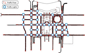
Figure 5: Overview of the Shenzhen (China) road network. There are total 33 traffic signal intersections across the area.

Table 1: Performance on the Common Testing Mode. The smaller evaluation values mean the better performances.

Model	Hangzhou			Jinan			Newyork			Shenzhen			Mean
	real	mixedlow	mixedhigh	real	mixedlow	mixedhigh	real	mixedlow	mixedhigh	real	mixedlow	mixedhigh
Random	727.05	1721.25	1794.85	836.53	1547.33	1733.49	1858.41	1865.32	2105.19	728.65	1775.37	1965.38	1554.90
MaxPressure	416.82	2449.00	2320.65	355.12	839.09	1218.13	380.42	488.25	1481.48	389.45	753.23	1387.87	1039.96
Fixedtime	718.29	1756.41	1787.58	814.09	1532.82	1739.69	1849.78	1865.33	2086.59	786.54	1705.16	1845.03	1540.61
FixedtimeOffset	736.63	1755.79	1725.17	854.40	1553.84	1720.45	1919.54	1901.23	2141.79	798.46	1886.32	2065.90	1588.29
SlidingFormula	441.80	1102.02	1241.17	576.71	759.58	1251.32	1096.32	986.64	1656.37	452.30	876.01	1347.31	982.30
SOTL	1209.26	2051.70	2062.49	1453.97	1779.60	1991.03	1890.55	1923.80	2140.15	1376.52	1902.73	2098.09	1823.32
Individual RL	743.00	1704.73	1819.57	843.63	1552.97	1745.07	1867.86	1869.44	2100.68	769.47	1753.28	1845.34	1551.25
MetaLight	480.77	1465.87	1576.32	784.98	984.02	1854.38	261.34	482.45	2145.49	694.83	954.25	2083.26	1147.33
PressLight	529.64	1538.64	1754.09	809.87	1173.74	1930.98	302.87	437.91	1846.76	639.04	834.09	1832.76	1135.87
CoLight	297.89	960.71	1077.29	511.43	733.10	1217.17	159.81	305.40	1457.56	438.45	657.55	1367.38	767.75
MetaVIM (w/o RS)	302.93	923.49	1643.98	593.30	837.49	1532.88	152.48	298.44	1834.73	426.48	676.23	1630.29	906.89
MetaVIM	284.28	893.98	986.74	492.04	694.56	1189.56	149.39	288.43	1387.93	408.28	622.46	1272.84	724.21

Experiments

A city-level open-source simulation platform CityFlow (?) is adopted to evaluate the method. More details of implementation such as the network architecture and hyper-parameters are list in the supplementary.

Settings

Datasets

The evaluation scenarios come from four real road networks of different scales, including Hangzhou (China), Jinan (China), New York (USA) and Shenzhen (China). The road networks and data of Hangzhou, Jinan and New York are from the public datasets The road network map of Shenzhen is derived from OpenStreetMap containing 33 traffic signal lights as shown in Fig. 5, and the traffic flow is generated based on the traffic trajectories collected from 80 red-light cameras and 16 monitoring cameras in a hour. There are 1,775 valid driving records in the span of 3600 seconds after data cleaning.

At each scenario, three three traffic flow configurations are employed including: (1) The real refers to the real one-hour traffic flow distribution. (2) The mixed_low which is a mixed traffic flow with a total flow of 2550 in one hour, in order to simulate a light peak. As shown in Fig. 6, the arrival rate of the traffic flow changes every 10 minutes, which is used to simulate the uneven traffic flow distribution in the real world. (3) The mixed_high is a mixed traffic flow with a total flow of 4770 in one hour, in order to simulate a heavy peak. The difference from the mixed_low setting is that the arriving rate of vehicles during 1200-1800s increased from 0.33 vehicles/s to 4.0 vehicles/s, which increased the arrival rate of vehicles during peak periods. In this scenario, there will be more vehicles accumulated in the road network.

Evaluation Criteria

The average travel time is adopted as the evaluation criteria, widely used in the field of transportation, which is the optimization goal of the Wardrop First Principle (UE, User Equilibrium) (?). That is, when reaching the user equilibrium state, the journey times in all routes actually used are less than those that would be experienced by a single vehicle on any unused route.

Testing Mode

The method is evaluated in two modes: 1) Common Testing Mode: the model trained on one scenario with one traffic flow configuration is tested on the same scenario with the same configuration. It is widely used to validate the ability of the RL algorithm to find the optimal policy; 2) Meta-Test Mode: we train the model in the Hangzhou road network and transfer the model to other three networks directly. It is used to validate the generality of the model.

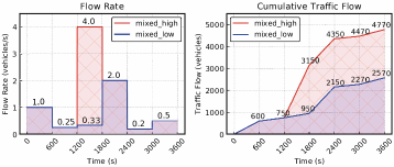
Figure 6: Illustration of mixed flow. The left figure shows the arrival rate of vehicles, and the right figure shows the cumulative number of vehicles arriving in one hour.

Table 2: Comparisons on the Meta-Test Mode. The original means the model is trained on the current testing scenario, and the transfer stands for the model is trained on the road map of Hangzhou.

Model	Jinan			Newyork			Shenzhen			Decline ratio
	real	mixedlow	mixedhigh	real	mixedlow	mixedhigh	real	mixedlow	mixedhigh
Individual RL (origin)	843.63	1552.97	1745.07	1867.86	1869.44	2100.68	769.47	1753.28	1845.34	—
Individual RL (transfer)	1198.46	2198.36	2493.46	2578.04	2330.65	2837.84	1046.37	2487.46	2513.89	38%
MetaLight (origin)	784.98	984.02	1854.38	261.34	482.45	2145.49	694.83	954.25	2083.26	—
MetaLight (transfer)	983.23	982.01	2287.46	316.69	593.20	2487.25	865.39	1139.48	2593.01	19%
PressLight (origin)	2593.01	1173.74	1930.98	302.87	437.91	1846.76	639.04	834.09	1832.76	—
PressLight (transfer)	1119.73	1703.54	2693.65	429.03	569.62	2376.54	906.47	1287.45	2673.89	41%
CoLight (origin)	511.43	733.10	1217.17	159.81	305.40	1457.56	438.45	657.55	1367.38	—
CoLight (transfer)	—	—	—	—	—	—	—	—	—	—
MetaVIM (origin)	492.04	694.56	1189.56	149.39	288.43	1387.93	408.28	622.46	1272.84	—
MetaVIM (transfer)	513.45	729.46	1362.91	153.87	341.89	1477.32	443.56	682.36	1401.63	9%

Comparisons

Baselines

We compare MetaVIM with 10 related baselines which are categorized into two types:

$\bullet$ Conventional methods (?) including Random where a phase is randomly selected from the candidate phases, MaxPressure (?) which is a leading conventional method and selects the phase by maximizing the pressure, Fixedtime which executes each phase in a phase loop with a pre-defined span of phase duration, FixedtimeOffset where multiple intersections use the same synchronized fix-time plan, SlidingFormula designed based on the expert experience, and SOTL (?) which is a self-organizing traffic light control method and chooses a plan among several candidate options.

$\bullet$ RL-based methods consist of Individual RL (?) which controls all agents independently based on DQN, CoLight (?) where the graph convolution and attention mechanism is employed to model the neighbors’ information, MetaLight (?) which is a value-based meta reinforcement learning method via parameter initialization, and PressLight (?) which combines the traditional traffic method MaxPressure with RL technology together.

These methods are evaluated under in the same setting for fairness, and their results are counted by running their source codes . All the baselines are evaluated under three different seeds, and the mean is taken as the final result. The action interval is five seconds for each method, and the horizon is 3600 seconds for each episode.

Evaluation on Common Testing

Table 5 lists the comparative results on the common testing mode, and it is evident that: 1) In general, RL methods perform better than convolutional methods, and it indicates the advantage of the RL. Moreover, MetaVIM is superior to other methods clearly in all scenarios and configurations, demonstrates the effectiveness of the method. 2) The MetaVIM shows good generalization for different scenarios and configurations. For example, MaxPressure and SlidingFormula perform good results in Hangzhou with the real configuration. While under the mixed_low and mixed_high traffic conditions, MaxPressure perform significantly worse than other methods. In contrast, MetaVIM can not only achieve good performance under diverse configurations of Hangzhou, but also shows great stability. 3) The MetaVIM outperforms Individual RL, MetaLight and PrssLight with 827.04, 423.12 and 411.66, respectively. The reason is that they learn the traffic light’s police only using its observation and ignore the influence of the neighbours, while the MetaVIM considering the neighbours as the unobserved part of the current light to help learning. 4) The neighbours’ information is modeled in CoLight and it performs well. The results of MetaVIM is superior to CoLight on each scenario and configuration, resulting mean 43.54 improvement. Compared to Colight, MetaVIM proposes an intrinsic reward to help the policies learning stable. In addition, Colight needs the communications among the agents in testing, which is unnecessary in MetaVIM. This makes MetaVIM easy to deploy.

Evaluation on Meta-Test

The comparative results evaluated on the meta-test mode is shown in Table 2. The “original” means the model is trained on the current testing scenario, and the “transfer” stands for the model is trained on the road map of Hangzhou. From the results, we can obtain follow findings: 1) Colight needs the whole state information in both training and testing, hence it cannot be used for a new scenario which contains different number intersections compared wit the training scenario. It indicates the necessity of learning the decentralized policy. 2) The performances of Individual RL and PressLight drop 38% and 41% when the model is transferred. It shows that the models learned by the common RL algorithms indeed rely on the training scenario. 3) MetaLight is more robust to different scenarios than Individual RL and PressLight, and it demonstrates the advantage of the meta-learning framework. Overall, MetaVIM achieve the state-of-the-art performance and only drops 9% when transferring the model. The reason is that the leaned latent variable $m_{i}$ can represent the task-specific information and helps to learn the across-task shared policy function better.

Ablations

For ablation studies, we compare with the variants of MetaVIM to verify the effectiveness of each component of MetaVIM. As illustrated in Table 5, we removed the intrinsic reward, only using the VAE part without using reward shaping as MetaVIM (w/o RS). Comparing MetaVIM and MetaVIM (w/o RS), results demonstrate that under real and mixed_low configurations, MetaVIM (w/o RS) performances are similar to the integral MetaVIM, only slightly weaker. However, when applied to mixed_high configuration, MetaVIM substantially outperforms MetaVIM (w/o RS) . This verifies that when the road network becomes more complicated and the dynamics of the road network increases, heuristic reward shaping via intrinsic reward is really effective, helping to learn more reasonable collaborative behaviors. If we removed the mVAE from the MetaVIM, then MetaVIM only has a policy network, and since Decoder is discarded, additive neighbours’ policies can not further be added in, the baseline is similar to independent control. Compared with Individual RL, MetaVIM achieves better performance, demonstrating mVAE could help agents obtain valuable information from the past trajectories and learn better policies. More analysis of other components are listed in the supplementary.

Conclusions

In this work, we propose a novel MetaVIM RL method to learn the decentralized polices in the traffic light control task. The MetaVIM makes three contributions. Firstly, the traffic signal control task is formulated as a meta-learning problem. The training scenario is divided into multiple POMDPs, where each POMDP corresponds to a traffic light and its neighbours are modeled as the unobserved part of the state. Secondly, a learned latent variable conditioned on the past trajectories is proposed for each task to represent the specific information, and helps to learn the POMDP-shared policy function. In addition, to make the policy learning stable, 4 decoders are introduced to predict the observations and rewards of each POMDP with/without neighbour agents’ policies, and a novel intrinsic reward is designed to encourage the predicted results invariant to the neighbours. Extensive experiments conducted on CityFlow demonstrate that the effectiveness and superior generalizability of MetaVIM.

Appendix A Supplementary Material of
“Meta Variationally Intrinsic Motivated Reinforcement Learning
for Decentralized Traffic Signal Control”

To better explain the method, we introduce more preliminaries of the traffic signal control task, the used notations in the main text, implementation details and more experimental results (especially the component analysis) in the supplementary material. In addition, the existing RL-based traffic signal control methods are listed in detail to clarify our contributions.

Appendix B Preliminary

Here we explain some concepts in the traffic signal control task.

Incoming/Outgoing Lanes

For an intersection, the incoming lanes refer to the lanes where the vehicles are about to enter the intersection as illustrated in Fig. 7. Generally, the direction of the incoming lanes depends on the driving direction. For example, the incoming lanes are on the right in China due to cars drive on the right-hand side of the road, while in the United States cars drive on the left-hand side of the road, hence the incoming lanes locate on the left side. Note that vehicles on the incoming lanes are affected by the traffic signal at the current intersection. However, the outgoing lanes are free from the influences induced by the traffic signal. For a three-lane road, the incoming lanes correspond to turning left, going straight and turning right from the middle to the side, respectively. For a four-leg intersection, 12 incoming lanes and 12 outgoing lanes are marked in Fig. 7.

Phase

Phase is a controller timing unit associated with the control of one or more movements, representing the permutation and combination of different traffic flows. A phase is a right-of-way, yellow change, and red chearance intervals in a cycle that are assigned to an independent traffic movement. The order of a series of phases called phase sequence.

Average Travel Time

The average travel time indicates the traffic situation at the intersection. A vehicle from the start point to the end point is regarded as a travel, and the sum of the time spending on the road including the stopped delay times is called the travel time. In a given period of time horizon, the average time spent by all vehicles is called the average travel time. Assuming that the driving speed of the vehicle is relatively stable, reasonable signal light control will reduce the delay time of the vehicles, the average travel time will decline correspondingly.

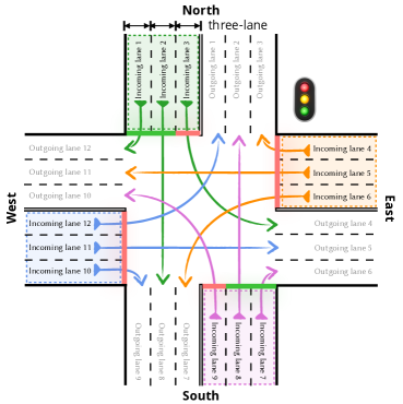
Figure 7: Illustration of incoming and outgoing lanes.

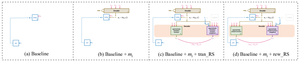
Figure 8: The evaluated models in the component analysis

Appendix C Notations

There are a few of mathematical symbols in the main text, and we conclude them in Table 3 to read the main text easily.

Appendix D Implementation Details

MetaVIM consists of a policy network and a multi-head variational autoencoder (mVAE), where the hyperparameters and specific network architecture used in the experiment are listed in Table  4.

During the learning, the replay buffer of policy network $\mathcal{D}^{\pi}$ collects the 60 most recent samples, and each sample contains the observation, action, reward, predicted action value, the latent mean and variable calculated by the encoder. The replay buffer of the mVAE $\mathcal{D}^{mVAE}$ maintains 100,000 trajectories. At every parallel processes time steps, $\mathcal{D}^{mVAE}$ collects the previous observation, current observation, action, task info about the current POMDP and the neighbor’s action.

Appendix E Experiments

Datasets Description

The road network map of Hangzhou (China), Jinan (China), New York (USA) and Shenzhen (China) are illustrated in Fig. 9. The road networks of Jinan and Hangzhou contain 12 and 16 intersections in $4\times 3$ and $4\times 4$ grids, respectively. The road network of New York includes 48 intersections in $16\times 3$ grid. The road network of Shenzhen contains 33 intersections, which is not grid compared to other three maps.

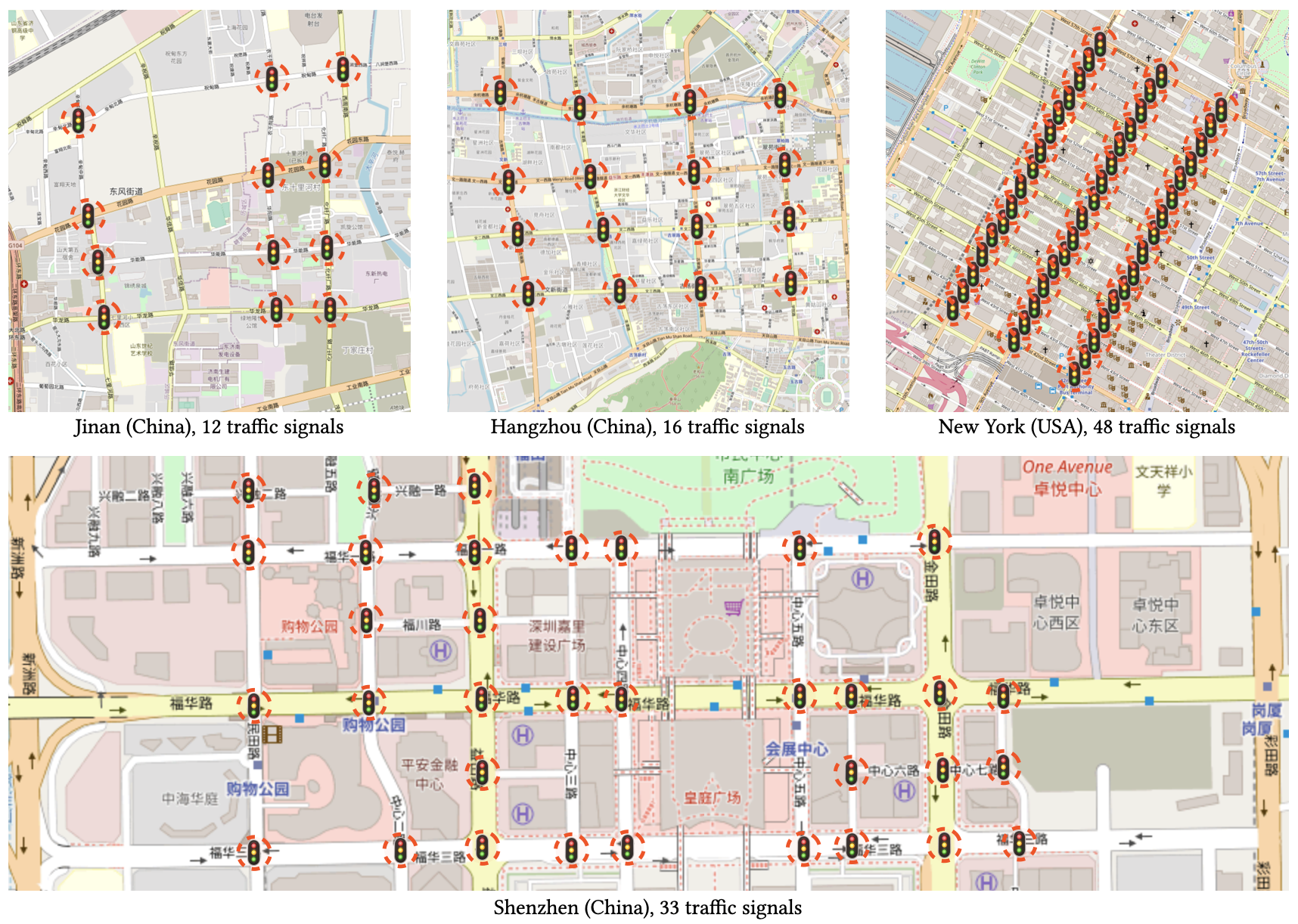
Figure 9: The illustration of the road networks. The first row shows the road networks of Jinan (China), Hangzhou (China) and New York (China), containing 12, 16 and 48 traffic signals respectively, and the second row shows the road network of Shenzhen containing 33 traffic signals.

Table 3: Notations

Component	Notation	Meaning
	$N$	number of traffic signals
	$\mathcal{O}_{i}$	a set of observations
	$\mathcal{S}_{i}$	a set of states
	$\mathcal{A}_{i}$	a set of actions
	$\mathcal{R}_{i}$	reward function
	$\mathcal{T}_{i}$	transition function
	$\mathcal{H}_{i}$	horizon (episode length)
	$t$	current time step
	$o_{i,t}$	$o_{i,t}\in\mathcal{O}_{i}$, the observation of agent $i$ at time step $t$
	$u_{i,t}$	$u_{i,t}=\{{o}_{i,t}^{-1},{a}_{t}^{-1}\}$, the unobserved part of agent $i$ at time step $t$
Policy	$s_{i,t}$	$s_{i,t}\in\mathcal{S}_{i}$, the POMDP state of agent $i$ at time step $t$,
	$a_{i,t}$	$a_{i,t}\in\mathcal{A}_{i}$, the action of agent $i$ at time step $t$
	$r_{i,t}$	the reward of agent $i$ for taking the action $a_{t}$ in current state
	${o}_{i,t}^{-1}$	the observations of the neighbours
	${a}_{i,t}^{-1}$	the actions of the neighbours
	$\pi^{\theta}_{i}(a_{i,t}|o_{i,t})$	policy of agent $i$
	$\theta$	the policy network parameter
	$u_{t}^{-j}$	the unobserved part of agent $i$
	$r^{int}_{t}$	intrinsic reward
	$\mathcal{D}^{\pi}$	replay buffer of the policy
	$i$	$i\in{0,1,...,N}$, a POMDP (a traffic signal)
	$\tau_{i,:t}$	past trajectories
	$m_{i}$	$m_{i}\sim\mathcal{N}(\mu_{i},\sigma_{i}^{2})$, latent variable
	$\mu_{i}$	mean of latent variable $m_{i}$
	$\sigma_{i}$	standard deviation of latent variable $m_{i}$
	$d_{i}(\cdot)$	multi-head decoder
	$p(m_{i}|\tau_{i,:t})$	posterior distribution
	$r_{t+1}$	predicted reward of decoder $p^{\phi_{r}}$
	$\tilde{r}_{j,t+1}$	predicted reward of decoder $p^{\phi_{\tilde{r}}}$
mVAE	$o_{t+1}$	predicted observation of decoder $p^{\phi_{o}}$
	$\tilde{o}_{j,t+1}$	$i^{th}$ predicted observation of decoder $p^{\phi_{\tilde{o}}}$
	$e^{\psi}(m_{i}|\tau_{i,:t})$	encoder
	$p^{\phi_{r}}(r_{t+1})$	a part of decoder, approximate reward function
	$p^{\phi_{\tilde{r}}}(\tilde{r}_{t+1})$	a part of decoder approximate reward function with neighbor’s policy
	$p^{\phi_{o}}(o_{t+1})$	a part of decoder, approximate observation function
	$p^{\phi_{\tilde{o}}}(\tilde{o}_{t+1})$	a part of decoder approximate observation function with neighbor’s policy
	$\rho_{i}$	trajectory distribution of POMDP $i$
	$\mathcal{D}^{mVAE}$	replay buffer of the mVAE
	$x(m)$	$x(m)\left(m\in L_{in}\right)$, the number of vehicles on each incoming lanes
Environment	$p$	phase
	$q_{t}$	queue length on each incoming lanes $q_{t}(m)$
	$j$	any neighbour agent of $i$

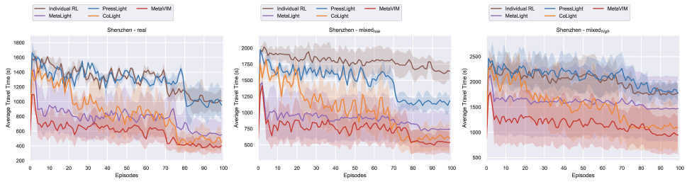
Figure 10: Learning curves of MetaVIM and other existing methods in the Shenzhen road network map. The first, second and third columns correspond to the real, mixed_low and mixed_high configurations respectively. Compared with Individual RL and PressLight, which can not capture the agent-to-agent helpful information thus to show poor performances, MetaVIM achieves better performance and shows great stability.

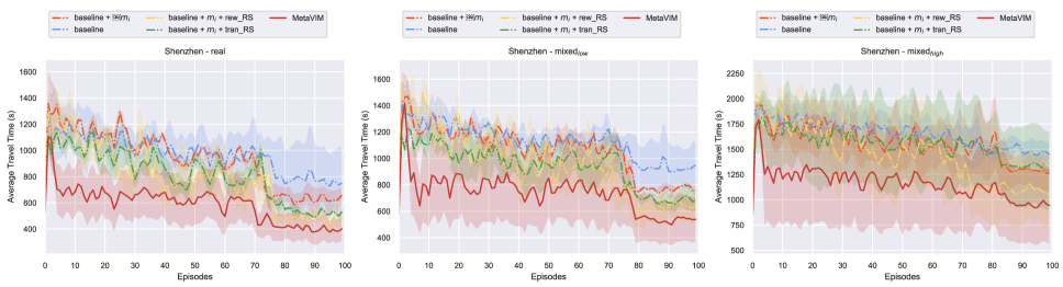
Figure 11: Learning curves of different models in the Shenzhen road network map. The final model MetaVIM outperforms all other models, and it indicates that each component contributes positively.

Table 4: Implementation details of MetaVIM

Number of policy steps	3600
Discount factor $\gamma$	0.95
Policy minibatch	16
mVAE minibatch	25
Value loss coefficient	0.5
Entropy coefficient	0.01
ELBO loss coefficient	1.0
Latent space dimensionality	5
Aggregator hidden size	64
Policy network architecture	2 hidden layers,
	32 nodes each,
	Tanh activations
Policy network optimizer	Adam with learning rate 0.0007 and epsilon 1e-5
Encoder architecture	FC layer with 40 nodes,
	GRU with hidden size 64,
	output layer with 10 outputs ($\mu$ and $\sigma$),
	ReLU activations
Transition Decoder architecture	2 hidden layers,
	32 nodes each,
	25 outputs heads,
	ReLU activations
Reward Decoder architecture	2 hidden layers,
	32 nodes each,
	25 outputs heads,
	ReLU activations
mVAE optimizer	Adam with learning rate 0.001 and epsilon 1e-5

Component Analysis

To better validate the contribution of each proposed component, five models are evaluated on the common testing mode in the Shenzhen road network map:

$\bullet$ Baseline (Fig. 8 (a)): We remove the mVAE and only keep the policy network, the latent variable $m_{i}$ is also removed from the input of the policy network;

$\bullet$ Baseline + $m_{i}$ (Fig. 8 (b)): The encoder is introduced and the latent variable $m_{i}$ is inputted to the policy network.

$\bullet$ Baseline + $m_{i}$ + tran_RS (Fig. 8 (c)): Based on Baseline + $m_{i}$, the transition encoders $\phi_{o}$ and $\phi_{\tilde{o}}$ are used to predict transitions, and only $\big{|}\big{|}o_{t+1}-\tilde{o}_{j,t+1}\big{|}\big{|}$ is remained in Eq. (3) of the main text;

$\bullet$ Baseline + $m_{i}$ + rew_RS (Fig. 8 (d)): Based on Baseline + $m_{i}$ + rew_RS, the reward encoders $\phi_{r}$ and $\phi_{\tilde{r}}$ are used to predict rewards, and only $\big{|}\big{|}r_{t+1}-\tilde{r}_{j,t+1}\big{|}\big{|}$ is remained in Eq. (3) of the main text;

$\bullet$ MetaVIM : The full model where all of the proposed components are employed, that is, it is equivalent to “Baseline + $m_{i}$ + tran_RS + rew_RS”. All of these 5 models are trained on a horizon of 3600 seconds for 100 episodes, respectively.

The qualitative evaluation results are listed in Table 5 and the learning curves are shown in Fig.  11. We can obtain the follow findings: 1) Among these 5 models, the performance of Baseline is the worst. The reason is that it is hard to learn the effective decentralized policy independently in the traffic light signal task, where one agent’s reward and transition are affected by its neighbours. 2) Compared with the baseline, the improvement of Baseline + $m_{i}$ demonstrates the effectiveness of the latent variable $m_{i}$. The latent variable not only identifies the POMDP-specific information and helps to learn POMDP-shared policy network, but also trades off the exploration and exploitation during the RL procedure. 3) The tran_RS and tran_RS are both effective because each of them encourages the policy learning stable. Compared to them, the superiority of MetaVIM indicates tran_RS and tran_RS are complementary to each other. 4) Overall, all of the proposed components contribute positively to the final model.

Table 5: Performances of different models on the Common Testing Mode. The smaller evaluation values mean the better performances.

Model	Hangzhou			Jinan			Newyork			Shenzhen			Mean
	real	mixedlow	mixedhigh	real	mixedlow	mixedhigh	real	mixedlow	mixedhigh	real	mixedlow	mixedhigh
Random	727.05	1721.25	1794.85	836.53	1547.33	1733.49	1858.41	1865.32	2105.19	728.65	1775.37	1965.38	1554.90
MaxPressure	416.82	2449.00	2320.65	355.12	839.09	1218.13	380.42	488.25	1481.48	389.45	753.23	1387.87	1039.96
Fixedtime	718.29	1756.41	1787.58	814.09	1532.82	1739.69	1849.78	1865.33	2086.59	786.54	1705.16	1845.03	1540.61
FixedtimeOffset	736.63	1755.79	1725.17	854.40	1553.84	1720.45	1919.54	1901.23	2141.79	798.46	1886.32	2065.90	1588.29
SlidingFormula	441.80	1102.02	1241.17	576.71	759.58	1251.32	1096.32	986.64	1656.37	452.30	876.01	1347.31	982.30
SOTL	1209.26	2051.70	2062.49	1453.97	1779.60	1991.03	1890.55	1923.80	2140.15	1376.52	1902.73	2098.09	1823.32
Individual RL	743.00	1704.73	1819.57	843.63	1552.97	1745.07	1867.86	1869.44	2100.68	769.47	1753.28	1845.34	1551.25
MetaLight	480.77	1465.87	1576.32	784.98	984.02	1854.38	261.34	482.45	2145.49	694.83	954.25	2083.26	1147.33
PressLight	529.64	1538.64	1754.09	809.87	1173.74	1930.98	302.87	437.91	1846.76	639.04	834.09	1832.76	1135.87
CoLight	297.89	960.71	1077.29	511.43	733.10	1217.17	159.81	305.40	1457.56	438.45	657.55	1367.38	767.75
baseline	526.38	1501.93	1674.98	793.84	1093.84	1904.93	298.48	432.94	1793.84	593.84	813.93	1732.94	1096.82
baseline+$m_{i}$	302.93	923.49	1643.98	593.30	837.49	1532.88	152.48	298.44	1834.73	426.48	676.23	1630.29	906.89
baseline+$m_{i}$+tran_RS	348.88	1134.09	1289.03	694.21	863.32	1406.92	189.22	368.90	1783.77	472.94	694.46	1416.13	888.49
baseline+$m_{i}$+rew_RS	338.48	1049.86	1274.94	683.58	849.85	1375.92	173.56	327.84	1738.95	453.94	683.94	1372.42	860.27
MetaVIM	284.28	893.98	986.74	492.04	694.56	1189.56	149.39	288.43	1387.93	408.28	622.46	1272.84	724.21

Appendix F RL based Traffic Signal Control Methods

Traditional signal control methods have many limitations. In recent years, there have been many research data-driven reinforcement learning methods. In a single agent environment, (?) introduces a phase gate on the basis of DQN in a simple two-phase scenario, and can select different sub-networks to generate decisions under different phases. (?) proposed the FRAP method, by introducing phase competition, priority is given to traffic signals with large traffic volume. (?) discusses the rationality of state design and reward design in the intelligent body on the problem of traffic signal control. It is not that good results can be achieved by repeatedly stacking some indicators, and finally a simplified design scheme can achieve good results in experiments. performance. (?) aims at the problem that RL methods are difficult to converge, and uses cases collected from classic methods to accelerate learning and achieve more effective exploration. In a multi-agent environment, (?) is an independent single-agent control method. The agent just greedily maximizes its reward, lacking communication and collaboration. (?) centrally optimizes multiple intersections to achieve collaboration, but the centralized method cannot be scaled to a more complex environment, because the state space and action space will explode in dimensionality. (?) is a decentralized method. With the help of graph convolutional neural network, the hidden state of neighbors is added, but it is only for self-decision. (?) adds multi-head attention on the basis of graph convolution. As the number of hops increases, the receptive field gradually expands, but these methods are not directly related to reward. (?), (?) and (?) use the max-pressure method to optimize the action with the largest throughput, which is a network-level control. (?) is a single-agent reinforcement learning method based on meta-learning. It learns the initialization parameters and applies it to each multi-agent scenario. Unlike them, instead of learning a set of initialization parameters, we learn embedding and implement rapid updates on this basis. In addition, we also added the estimated errors between the enlightening Decoders as intrinsic rewards, resulting in more collaborative behaviors.

References

- [Andrychowicz et al. 2017] Andrychowicz, M.; Wolski, F.; Ray, A.; Schneider, J.; Fong, R.; Welinder, P.; McGrew, B.; Tobin, J.; Abbeel, O. P.; and Zaremba, W. 2017. Hindsight experience replay. In Advances in neural information processing systems.
- [Bellemare et al. 2016] Bellemare, M.; Srinivasan, S.; Ostrovski, G.; Schaul, T.; Saxton, D.; and Munos, R. 2016. Unifying count-based exploration and intrinsic motivation. In Advances in neural information processing systems.
- [Chen et al. 2020] Chen, C.; Wei, H.; Xu, N.; Zheng, G.; Yang, M.; Xiong, Y.; Xu, K.; and Li, Z. 2020. Toward a thousand lights: Decentralized deep reinforcement learning for large-scale traffic signal control. In AAAI.
- [Chitnis et al. 2020] Chitnis, R.; Tulsiani, S.; Gupta, S.; and Gupta, A. 2020. Intrinsic motivation for encouraging synergistic behavior. arXiv preprint arXiv:2002.05189.
- [Cools, Gershenson, and D’Hooghe 2013] Cools, S.-B.; Gershenson, C.; and D’Hooghe, B. 2013. Self-organizing traffic lights: A realistic simulation. In Advances in applied self-organizing systems. Springer.
- [Dafermos and Sparrow 1969] Dafermos, S. C., and Sparrow, F. T. 1969. The traffic assignment problem for a general network. Journal of Research of the National Bureau of Standards B 73(2).
- [El-Tantawy, Abdulhai, and Abdelgawad 2013] El-Tantawy, S.; Abdulhai, B.; and Abdelgawad, H. 2013. Multiagent reinforcement learning for integrated network of adaptive traffic signal controllers (marlin-atsc): methodology and large-scale application on downtown toronto. IEEE Transactions on Intelligent Transportation Systems 14(3):1140–1150.
- [Foerster et al. 2017] Foerster, J.; Farquhar, G.; Afouras, T.; Nardelli, N.; and Whiteson, S. 2017. Counterfactual multi-agent policy gradients. arXiv preprint arXiv:1705.08926.
- [Humplik et al. 2019] Humplik, J.; Galashov, A.; Hasenclever, L.; Ortega, P. A.; Teh, Y. W.; and Heess, N. 2019. Meta reinforcement learning as task inference. arXiv preprint arXiv:1905.06424.
- [Jaques et al. 2019] Jaques, N.; Lazaridou, A.; Hughes, E.; Gulcehre, C.; Ortega, P.; Strouse, D.; Leibo, J. Z.; and De Freitas, N. 2019. Social influence as intrinsic motivation for multi-agent deep reinforcement learning. In International Conference on Machine Learning. PMLR.
- [Kingma and Welling 2013] Kingma, D. P., and Welling, M. 2013. Auto-encoding variational bayes. arXiv preprint arXiv:1312.6114.
- [Koonce and Rodegerdts 2008] Koonce, P., and Rodegerdts, L. 2008. Traffic signal timing manual. Technical report, United States. Federal Highway Administration.
- [Kuyer et al. 2008] Kuyer, L.; Whiteson, S.; Bakker, B.; and Vlassis, N. 2008. Multiagent reinforcement learning for urban traffic control using coordination graphs. In Joint European Conference on Machine Learning and Knowledge Discovery in Databases. Springer.
- [Lowe et al. 2017] Lowe, R.; Wu, Y. I.; Tamar, A.; Harb, J.; Abbeel, O. P.; and Mordatch, I. 2017. Multi-agent actor-critic for mixed cooperative-competitive environments. In Advances in neural information processing systems.
- [Mannion, Duggan, and Howley 2016] Mannion, P.; Duggan, J.; and Howley, E. 2016. An experimental review of reinforcement learning algorithms for adaptive traffic signal control. In Autonomic road transport support systems. Springer.
- [Modi and Tewari 2019] Modi, A., and Tewari, A. 2019. Contextual markov decision processes using generalized linear models.
- [Nishi et al. 2018] Nishi, T.; Otaki, K.; Hayakawa, K.; and Yoshimura, T. 2018. Traffic signal control based on reinforcement learning with graph convolutional neural nets. In 2018 21st International Conference on Intelligent Transportation Systems (ITSC). IEEE.
- [Oliehoek, Amato, and others 2016] Oliehoek, F. A.; Amato, C.; et al. 2016. A concise introduction to decentralized POMDPs, volume 1. Springer.
- [Ortega et al. 2019] Ortega, P. A.; Wang, J. X.; Rowland, M.; Genewein, T.; Kurth-Nelson, Z.; Pascanu, R.; Heess, N.; Veness, J.; Pritzel, A.; Sprechmann, P.; et al. 2019. Meta-learning of sequential strategies. arXiv preprint arXiv:1905.03030.
- [Pathak et al. 2017] Pathak, D.; Agrawal, P.; Efros, A. A.; and Darrell, T. 2017. Curiosity-driven exploration by self-supervised prediction. In Proceedings of the IEEE Conference on Computer Vision and Pattern Recognition Workshops.
- [Rakelly et al. 2019] Rakelly, K.; Zhou, A.; Finn, C.; Levine, S.; and Quillen, D. 2019. Efficient off-policy meta-reinforcement learning via probabilistic context variables. In International conference on machine learning.
- [Rashid et al. 2018] Rashid, T.; Samvelyan, M.; De Witt, C. S.; Farquhar, G.; Foerster, J.; and Whiteson, S. 2018. Qmix: Monotonic value function factorisation for deep multi-agent reinforcement learning. arXiv preprint arXiv:1803.11485.
- [Schulman et al. 2017] Schulman, J.; Wolski, F.; Dhariwal, P.; Radford, A.; and Klimov, O. 2017. Proximal policy optimization algorithms. arXiv preprint arXiv:1707.06347.
- [Son et al. 2019] Son, K.; Kim, D.; Kang, W. J.; Hostallero, D. E.; and Yi, Y. 2019. Qtran: Learning to factorize with transformation for cooperative multi-agent reinforcement learning. arXiv preprint arXiv:1905.05408.
- [Sukhbaatar et al. 2017] Sukhbaatar, S.; Lin, Z.; Kostrikov, I.; Synnaeve, G.; Szlam, A.; and Fergus, R. 2017. Intrinsic motivation and automatic curricula via asymmetric self-play. arXiv preprint arXiv:1703.05407.
- [Sunehag et al. 2018] Sunehag, P.; Lever, G.; Gruslys, A.; Czarnecki, W. M.; Zambaldi, V. F.; Jaderberg, M.; Lanctot, M.; Sonnerat, N.; Leibo, J. Z.; Tuyls, K.; et al. 2018. Value-decomposition networks for cooperative multi-agent learning based on team reward. In AAMAS.
- [Tan 1993] Tan, M. 1993. Multi-agent reinforcement learning: Independent vs. cooperative agents. In Proceedings of the tenth international conference on machine learning.
- [Van der Pol and Oliehoek 2016] Van der Pol, E., and Oliehoek, F. A. 2016. Coordinated deep reinforcement learners for traffic light control. Proceedings of Learning, Inference and Control of Multi-Agent Systems (at NIPS 2016).
- [Varaiya 2013] Varaiya, P. 2013. The max-pressure controller for arbitrary networks of signalized intersections. In Advances in Dynamic Network Modeling in Complex Transportation Systems. Springer.
- [Wei et al. 2018] Wei, H.; Zheng, G.; Yao, H.; and Li, Z. 2018. Intellilight: A reinforcement learning approach for intelligent traffic light control. In Proceedings of the 24th ACM SIGKDD International Conference on Knowledge Discovery & Data Mining.
- [Wei et al. 2019a] Wei, H.; Chen, C.; Zheng, G.; Wu, K.; Gayah, V.; Xu, K.; and Li, Z. 2019a. Presslight: Learning max pressure control to coordinate traffic signals in arterial network. In Proceedings of the 25th ACM SIGKDD International Conference on Knowledge Discovery & Data Mining.
- [Wei et al. 2019b] Wei, H.; Xu, N.; Zhang, H.; Zheng, G.; Zang, X.; Chen, C.; Zhang, W.; Zhu, Y.; Xu, K.; and Li, Z. 2019b. Colight: Learning network-level cooperation for traffic signal control. In Proceedings of the 28th ACM International Conference on Information and Knowledge Management.
- [Xiong et al. 2019] Xiong, Y.; Zheng, G.; Xu, K.; and Li, Z. 2019. Learning traffic signal control from demonstrations. In Proceedings of the 28th ACM International Conference on Information and Knowledge Management.
- [Zang et al. 2020] Zang, X.; Yao, H.; Zheng, G.; Xu, N.; Xu, K.; and Li, Z. 2020. Metalight: Value-based meta-reinforcement learning for traffic signal control. In Proceedings of the AAAI Conference on Artificial Intelligence, volume 34.
- [Zhang et al. 2019] Zhang, H.; Feng, S.; Liu, C.; Ding, Y.; Zhu, Y.; Zhou, Z.; Zhang, W.; Yu, Y.; Jin, H.; and Li, Z. 2019. Cityflow: A multi-agent reinforcement learning environment for large scale city traffic scenario. In The World Wide Web Conference.
- [Zheng et al. 2019a] Zheng, G.; Xiong, Y.; Zang, X.; Feng, J.; Wei, H.; Zhang, H.; Li, Y.; Xu, K.; and Li, Z. 2019a. Learning phase competition for traffic signal control. In Proceedings of the 28th ACM International Conference on Information and Knowledge Management.
- [Zheng et al. 2019b] Zheng, G.; Zang, X.; Xu, N.; Wei, H.; Yu, Z.; Gayah, V.; Xu, K.; and Li, Z. 2019b. Diagnosing reinforcement learning for traffic signal control. arXiv preprint arXiv:1905.04716.
- [Zintgraf et al. 2019a] Zintgraf, L.; Shiarli, K.; Kurin, V.; Hofmann, K.; and Whiteson, S. 2019a. Fast context adaptation via meta-learning. In International Conference on Machine Learning. PMLR.
- [Zintgraf et al. 2019b] Zintgraf, L.; Shiarlis, K.; Igl, M.; Schulze, S.; Gal, Y.; Hofmann, K.; and Whiteson, S. 2019b. Varibad: A very good method for bayes-adaptive deep rl via meta-learning. arXiv preprint arXiv:1910.08348.