Exact Coverage Analysis of Intelligent Reflecting Surfaces with Nakagami-m Channels

Abstract

Intelligent Reflecting Surfaces (IRS) are a promising solution to enhance the coverage of future wireless networks by tuning low-cost passive reflecting elements (referred to as metasurfaces), thereby constructing a favorable wireless propagation environment. Different from prior works, which assume Rayleigh fading channels and do not consider the direct link between a base station and a user, this article develops a framework based on moment generation functions (MGF) to characterize the coverage probability of a user in an IRS-aided wireless systems with generic Nakagami-m fading channels in the presence of direct links. In addition, we demonstrate that the proposed framework is tractable for both finite and asymptotically large values of the metasurfaces. Furthermore, we derive the channel hardening factor as a function of the shape factor of Nakagami-m fading channel and the number of IRS elements. Finally, we derive a closed-form expression to calculate the maximum coverage range of the IRS for given network parameters. Numerical results obtained from Monte-Carlo simulations validate the derived analytical results.

I Introduction

Intelligent reflecting surfaces (IRSs) are considered as among one of the key enabling technologies for 6G wireless networks. IRSs are fabricated surfaces of electromagnetic (EM) material that are electronically controlled with integrated electronics and have unique wireless communication capabilities. IRSs do not need any power supply, complex signal processing, or encoding and decoding processes, which are especially used to improve the signal quality at the receiver [1, 2]. IRSs enable telecommunication operators to create a controllable channel propagation environment [3]. Recent results have revealed that reconfigurable intelligent surfaces can effectively control the wavefront, e.g., the phase, amplitude, frequency, and even polarization, of the impinging signals without complex signal processing operations.

Recently, a handful of research works have considered the coverage analysis of a user, assuming IRS-only transmissions with no direct transmission link between a base station (BS) and a user [4, 5, 6, 2, 7, 8, 9, 10]. For instance, Ertugrul et al. [2] proposed a preliminary model to characterize the bit error rate of an IRS-assisted communication system with large number of IRS elements and applied central limit theorem (CLT). Yang et al. [4] characterized the coverage of an IRS-aided communication system with large number of IRS elements, applied CLT, and compared it with the relaying systems using Rayleigh fading channels. Zhang et al. [5] investigated the downlink performance of IRS-aided non-orthogonal multiple access (NOMA) networks via stochastic geometry. Yue and Liu [6] investigated the coverage probability in an IRS-assisted downlink NOMA networks.

Samuh and Salhab [7] approximated the outage probability, average symbol error probability (ASEP), and average channel capacity using the first term of Laguerre expansion. Trigui et al. [8] derived the outage and ergodic capacity considering generalized Fox’H fading channel. The expressions are in the form of multi-integral expressions and closed-forms are in the form of multi-variate Fox’H functions. Considering Nakagami-m fading channels, Ferreira et al. [9] derived the exact bit error probability considering quadrature amplitude and binary phase-shift keying (BPSK) modulations when the number of IRS elements, $n$, is equal to 2 and 3. The IRS-aided channel distributions for two and three IRS elements are given in the form of double and quadruple integrals, respectively. For large values of $n$, central limit theorem (CLT) was applied. Sharma and Garg [10] investigated the performance of IRSs with full duplex technology in terms of outage and error probabilities. The authors considered Nakagami-m fading channels and applied CLT.

None of the aforementioned research considered direct links; therefore, it is difficult to identify scenarios in which IRS-assisted transmissions outperform direct transmissions. Furthermore, most existing works assumed asymptotically large numbers of IRS elements and leverage on CLT [11, 6]. Recently, Lyu and Zhang [11] derived the spatial user throughput considering Rayleigh fading, taking into account direct links. However, to avoid tedious convolution of the probability density functions (PDFs) of the direct link and IRS-aided link, they approximated the PDF of the cumulative channel gain using instead of with the gamma distribution.

Different from the aforementioned works, our contributions can be summarized as follows:

• We provide a comprehensive moment generating function (MGF)-based framework to derive the exact coverage probability of a user in an IRS-aided wireless system, assuming generic Nakagami-m fading channels in the presence of direct link.

• The proposed framework is analytically tractable for both finite and asymptotically large numbers of the IRS elements, while allowing single integral coverage probability expressions. In contrast to CLT-based approximations or moment-based Gamma approximations, the proposed MGF-based approach can accurately reflect the behavior of IRS-assisted communication in all operating regimes.

• Furthermore, we derive the channel hardening factor as a function of the shape parameter of Nakagami-m fading channel and the number of IRS elements. The channel hardening factor reveals the conditions under which the channel becomes nearly deterministic, resulting in improved reliability and less frequent channel estimation.

• We derive a closed-form expression to calculate the maximum coverage of the IRS for the given network parameters.

• Numerical results obtained from Monte-Carlo simulations validate the analytical results and obtain useful insights related to the impact of a finite number of IRS elements, channel hardening in IRS-aided Nakagami-faded transmissions, the coverage range of the IRS, and the scenarios in which IRS-aided transmission gains can exceed direct transmission gains.

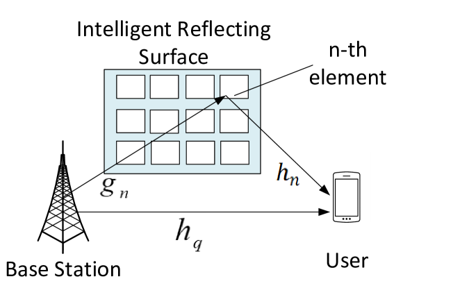
Figure 1: Intelligent reflecting surface-aided wireless system.

II System Model and Assumptions

We consider a downlink IRS-aided communication system composed of a BS, a user, and an IRS equipped with $N$ reflecting metasurfaces (as shown in Fig. 1). The BS and user are equipped with only one antenna. We assume that the IRS is placed between the BS and user to improve the user’s signal quality in the presence of direct transmissions. We assume that the IRS can obtain the full channel state information (CSI) to compute the phase shifts that maximize the signal-to-noise ratio (SNR) at the receiver [12, 13, 2].

Let $\mathbf{g}\overset{\Delta}{=}[g_{1},...,g_{N}]^{T}\in\mathbb{C}^{N\times 1}$, $\mathbf{h}\overset{\Delta}{=}[h_{1},...,h_{N}]^{T}\in\mathbb{C}^{N\times 1}$, and $h_{q}\in\mathbb{C}$ denote the baseband equivalent channels from the BS to the IRS, from the IRS to the user equipment (UE), and from the BS to the UE, respectively. Let $\mathbf{\Phi}\overset{\Delta}{=}\mathrm{diag}\{[e^{j\phi_{1}},...,e^{j\phi_{N}}]\}$ denote the phase-shifting matrix of the IRS, where $\phi_{n}\in[0,2\pi)$ is the phase shift by element $n$ on the incident signal, and $j$ denotes the imaginary unit. The cascaded BS-IRS-UE channel is then modeled as a concatenation of three components, namely, the BS-IRS spatial stream link, IRS reflecting with phase shifts, and the IRS-UE link, and given by [14] as $h_{c}\overset{\Delta}{=}\mathbf{g}^{T}\mathbf{\Phi}\mathbf{h}$. Note that the cascaded channel phase $\angle(g_{n}h_{n})$ for each IRS element $n=[1,...,N]$ can be obtained via channel estimation. The IRS then adjusts the phase shift $\boldsymbol{\phi}=[\phi_{1},...,\phi_{N}]$ such that the $N$ reflected signals are of the same phase at its served UE’s receiver by setting $\phi_{n}=-\angle(g_{n}h_{n})$, $n=1,...,N$. Therefore, the overall cascaded channel gain is as follows:

$$|h_{c}|=|\mathbf{g}|^{T}|\mathbf{h}|=\sum_{n=1}^{N}|g_{n}||h_{n}|.$$ (1)

We assume that the BS-UE channel phase $\angle h_{q}$ is also known and the IRS can perform a common phase-shift such that $h_{c}$ and $h_{q}$ are co-phased and hence coherently combined at the UE [4], with the overall channel amplitude denoted by

$$T=|h_{c}|+|h_{q}|.$$ (2)

We denote $l$, $r$ and $d$ as the BS-UE, BS-IRS and UE-IRS distances, respectively. The channel amplitude from the BS to the $n$-th element of IRS and from the $n$-th element of the IRS to the UE can then be modeled, respectively, as follows:

$$|g_{n}|\overset{\Delta}{=}\zeta^{1/2}\varepsilon_{g}r_{n}^{-\alpha/2},|h_{n}| \overset{\Delta}{=}\zeta^{1/2}\varepsilon_{h}d_{n}^{-\alpha/2}.$$ (3)

Similarly, the BS-UE channel amplitude is modeled as follows:

$$|h_{q}|\overset{\Delta}{=}\zeta\varepsilon_{q}l^{-\alpha/2},$$ (4)

where path-loss exponent $\alpha\geq 2$ and $\zeta=(\frac{\text{carrier wavelength}}{4\pi})^{2}$ is the near-field path loss factor at a reference distance of one meter (1 m) as a function of the carrier frequency. The distribution of the Nakagami-m fading channel gain $\varepsilon_{x}$ is thus given as follows:

$$f_{\varepsilon_{x}}(x)=\frac{2m^{m}x^{2m-1}}{\Omega^{m}\Gamma(m)}\exp\left(\frac{-mx^{2}}{\Omega}\right),x>0,$$ (5)

where $x\in\{g,h,q\}$ denotes the BS-IRS, IRS-UE and BS-UE links, respectively, and $\Gamma(.)$ is the gamma function. The fading severity parameter is $m\in[1,2,...,\infty)$ and the mean fading power is denoted by $\Omega$. Note that $m\geq 0.5$ is the shape (or fading figure) parameter. Rayleigh fading is a special case of Nakagami-m when $m=1$.

Let $P$ denote the BS downlink transmit power for each UE. If the typical UE is served by the BS only, then its received SNR can be modeled as follows:

$$\mathrm{SNR}_{B}\overset{\Delta}{=}P|h_{q}|^{2}\hat{\sigma}^{-2}=P\zeta\varepsilon_{q}l^{-\alpha}\hat{\sigma}^{-2},$$ (6)

where $l=\sqrt{r^{2}+d^{2}-2rd\cos{({\color[rgb]{0,0,0}\psi})}}$ and ${\color[rgb]{0,0,0}\psi}$ is the angle between the BS-IRS and IRS-UE link, and $\hat{\sigma}^{2}$ is the variance of the additive white Gaussian noise at the UE receiver. On the other hand, if the UE is served by both the IRS and BS, then its received SNR can be modeled as follows:

$$\mathrm{SNR}_{S} \overset{\Delta}{=}P(|h_{c}|+|h_{q}|)^{2}\hat{\sigma}^{-2}=P\left(\sum_{n=1}^{N}|g_{n}||h_{n}|+|h_{q}|\right)^{2}\hat{\sigma}^{-2}.$$

III Exact Coverage Probability Analysis

The coverage probability is defined by the complementary cumulative distribution function (CCDF) of the SNR (i.e., $\mathbb{P}[{\rm SNR}>\theta]$, where $\theta$ denotes the predefined threshold for correct signal reception) and is characterized as follows:

$$\mathcal{C}_{S} =\mathbb{P}[{\rm SNR_{S}}>\theta]=\mathbb{P}[P(|h_{c}|+|h_{q}|)^{2}\hat{\sigma}^{-2}>\theta],$$

$$={\color[rgb]{0,0,0}\mathbb{P}\Big{[}T>\left(\frac{\theta\hat{\sigma}^{2}}{P}\right)^{1/2}\Big{]}=1-F_{T}\left(\left(\frac{\theta\hat{\sigma}^{2}}{P}\right)^{1/2}\right)},$$ (7)

where $F_{T}(.)$ is the CDF of $T$. Following is our methodology: (i) deriving the Laplace transform (or moment generating function (MGF)) of $h_{c}$, $h_{q}$, and $T$ considering asymptotically large values of reflecting elements $N$ in Section III.A and finite values of $N$ in Section III.B, (ii) deriving the characteristic function (CF) of $T$, and (iii) applying Gil-Pelaez inversion to the CF of $T$.

III-A Asymptotically Large Values of Reflecting Elements $N$

The channel amplitude of the BS-IRS-UE signal that goes through element $n$ follows scaled double Nakagami-m, i.e.,

$$|h_{c}|\stackrel{{\scriptstyle(a)}}{{\approx}}\zeta r^{-\alpha/2}d^{-\alpha/2}\sum_{n=1}^{N}Y_{n}=\rho(r,d)\sum_{n=1}^{N}\varepsilon_{g}\varepsilon_{h},$$

where (a) follows from the limited size of the UE and the IRS, i.e., $d_{n}\approx d$ and $r_{n}\approx r$. Note that $Y_{n}$ denotes a double Nakagami-m distributed random variable with independent but not necessarily identically distributed (i.n.i.d) $\varepsilon_{h}$ and $\varepsilon_{g}$ variables and $\rho(r,d)=\zeta r^{-\alpha/2}d^{-\alpha/2}$.

For large values of $N$, the PDF of $|h_{c}|$ can be derived as:

$${h_{c}}\stackrel{{\scriptstyle(a)}}{{\approx}}\mathcal{N}\left(\rho(r,d)N\mathbb{E}[Y_{n}],\rho(r,d)^{2}N\mathrm{var}\{Y_{n}\}\right),$$ (8)

where $\mathcal{N}(\mu,\sigma^{2})$ denotes the Gaussian random variable with mean $\mu$ and variance $\sigma^{2}$. Note that step (a) follows from applying the central limit theorem (CLT) which dictates that $\sum_{n=1}^{N}Y_{n}$ approaches normal distribution as $N\rightarrow\infty$ and scaling the normal distribution with $\rho(r,d)$. The distribution of a normal random variable $X$ scaled with a constant $c$ is given by $cX\sim\mathcal{N}(c\mu,c^{2}\sigma^{2})$, where $\mu$ is the mean and $\sigma^{2}$ is the variance. The $b$-th order moment of a double Nakagami-m RV $Y_{n}$ can be given as [15]:

$$\mathbb{E}[Y_{n}^{b}]=\prod_{i=1}^{2}\frac{\Gamma(m_{i}+b/2)}{\Gamma(m_{i})}\left(\frac{\Omega_{i}}{m_{i}}\right)^{b/2}.$$ (9)

Therefore, the mean and variance of $Y_{n}$ are as follows:

$$\mu_{Y}=\mathbb{E}[Y_{n}]\overset{\Delta}{=}\prod_{i=1}^{2}\frac{\Gamma(m_{i}+1/2)}{\Gamma(m_{i})}\left(\frac{\Omega_{i}}{m_{i}}\right)^{1/2},$$

$$\sigma_{Y}^{2}=\mathrm{var}\{Y_{n}\}\overset{\Delta}{=}\mathbb{E}[Y_{n}^{2}]-\mathbb{E}[Y_{n}]^{2}=$$

$$=\prod_{i=1}^{2}\frac{\Gamma(m_{i}+1)}{\Gamma(m_{i})}\left(\frac{\Omega_{i}}{m_{i}}\right)-\left(\prod_{i=1}^{2}\frac{\Gamma(m_{i}+1/2)}{\Gamma(m_{i})}\left(\frac{\Omega_{i}}{m_{i}}\right)^{1/2}\right)^{2}.$$

Now given the distribution of $|h_{c}|$, the coverage probability can be derived as in the following lemma.

Lemma 1.

Applying the Gil-Pelaez inversion[16], the coverage probability can be obtained as $\mathcal{C}_{S}=1-F_{T}(t),$ where

$$F_{T}(t)=\frac{1}{2}+\frac{1}{\pi}\int_{0}^{\infty}\frac{\Im\left(e^{j\omega t}\varphi_{T}(\omega)\right)}{\omega}\text{d}\omega,$$ (10)

where $\Im(w)$ is imaginary part of $w\in\mathbb{C}$ and $j\overset{\Delta}{=}\sqrt{-1}$. The characteristic function of $T$ can be given as follows:

$$\varphi_{T}(\omega)=e^{-\mu_{Y}j\omega-\frac{1}{2}\sigma_{Y}^{2}\omega^{2}}\frac{\Gamma(m+0.5)}{\sqrt{\pi}}U\left(m,0.5,\frac{-(c_{1}\omega)^{2}\Omega}{4m}\right).$$

Proof.

Since $h_{q}$ is a scaled Nakagami-m distributed random variable, we first characterize the MGF of Nakagami-m variable $M_{Z}(s)$ as follows:

$$M_{Z}(s) =\int_{0}^{\infty}\frac{2m^{m}{Z}^{2m-1}}{\Omega^{m}\Gamma(m)}\exp\left(\frac{-m{Z}^{2}}{\Omega}\right)\exp(-sZ)dZ,$$

$$=\frac{1}{\sqrt{\pi}}\Gamma(m+0.5)U\left(m,0.5,\frac{s^{2}\Omega}{4m}\right),$$ (11)

where $U(a,b,z)$ is the confluent hypergeometric function. On the other hand, since we characterize $h_{c}$ as normally distributed after applying CLT in Eq. (8), the MGF of normally distributed variable $M_{h_{c}}(s)$ can be given as follows:

$$M_{h_{c}}(s) =\exp\left(-\mu_{Y}s+\frac{1}{2}\sigma_{Y}^{2}s^{2}\right).$$ (12)

Since $|h_{c}|$ and $|h_{q}|$ are independent, the MGF of $T=|h_{c}|+|h_{q}|$ can be obtained by the multiplication of the MGFs of the random variables $h_{c}$ and $h_{q}$ as follows:

$$M_{T}(s){=}M_{h_{c}}(s)M_{h_{q}}(s)\stackrel{{\scriptstyle(a)}}{{=}}M_{h_{c}}(s)M_{Z}(c_{1}s),$$ (13)

where step (a) follows from the scaling property of MGF $M_{h_{q}}(c_{1}s)$ which is scaled with constant $c_{1}$, where $|h_{q}|\overset{\Delta}{=}\zeta^{1/2}l^{-\alpha/2}\varepsilon_{q}^{1/2}=c_{1}\varepsilon_{q}^{1/2}$ and $c_{1}\overset{\Delta}{=}\zeta^{1/2}l^{-\alpha/2}$. ∎

For Rayleigh fading channels, the MGF of $T$ can be simplified as in the following corollary.

Corollary 1.

For $m=1$, the direct channel $h_{q}$ becomes scaled Rayleigh distributed random variable. Thus, using the identity $U(1,0.5,z)=e^{z}z^{0.5}\Gamma(-0.5,z)$, $M_{Z}(s)$ in Lemma 1 can be simplified as follows:

$$M_{Z}(s)=1-\frac{s\sqrt{\pi\Omega}}{2}e^{\frac{s^{2}\Omega}{4}}\mathrm{erfc}\left(\frac{s\sqrt{\Omega}}{2}\right),$$ (14)

where erfc($\cdot$) is the complementary error function.

III-B Finite Values of Reflecting Elements $N$

When $N$ is not a sufficiently large value, i.e., a finite value, the coverage probability $\mathcal{C}_{S}=1-F_{T}(t)$ can be characterized via the following lemma.

Lemma 2.

For finite values of $N$, we characterize the MGF of $|h_{c}|=\zeta r^{-\alpha/2}d^{-\alpha/2}\sum_{n=1}^{N}Y_{n}$ considering that $Y_{n}$ is independent for all $n$, i.e.,

$$M_{h_{c}}(c_{2}s)=\prod_{n=1}^{N}M_{Y_{n}}(c_{2}s),$$ (15)

where $c_{2}=\zeta r^{-\alpha/2}d^{-\alpha/2}$ is the scaling factor. Since $Y_{n}$ is a double Nakagami-m RV, its MGF can be given as follows [15]:

$$M_{Y_{n}}(s)=\frac{1/\sqrt{\pi}}{\prod_{i=1}^{2}\Gamma(m_{i})}G_{2,2}^{2,2}\Bigg{[}\frac{4}{s^{2}}\prod_{i=1}^{2}\frac{m_{i}}{\Omega_{i}}\Bigg{|}\begin{matrix}1/2&1\\ m_{1}&m_{2}\end{matrix}\Bigg{]},$$ (16)

where $G[\cdot]$ is the Meijer’s G-function [17].

For independent and identically distributed (i.i.d.) $\varepsilon_{g}$ and $\varepsilon_{h}$, we simplify the MGF of $|h_{c}|$ as follows.

Corollary 2.

For i.i.d. $\varepsilon$, $Y_{n}$ follows a Gamma distribution, the MGF of $h_{c}$ can thus be given as follows [18]:

$$M_{h_{c}}(c_{2}s)=\left(1+\frac{c_{2}s\Omega}{m}\right)^{-Nm}.$$ (17)

Since $|h_{c}|$ and $|h_{q}|$ are independent, the MGF of $T=|h_{c}|+|h_{q}|$ can be obtained as follows:

$$M_{T}(s){=}M_{h_{c}}(c_{2}s)M_{h_{q}}(s)\stackrel{{\scriptstyle(a)}}{{=}}M_{h_{c}}(c_{2}s)M_{Z}(c_{1}s),$$ (18)

where step (a) follows from substituting $M_{h_{q}}(s)$ given in Eq. (III-A). The coverage probability can then be obtained using Gil-Pelaez inversion in Lemma 1.

III-C Channel Hardening for Double Nakagami-m Channels

Let $\kappa$ denote the ratio between the mean $\mu_{Y}$ and standard deviation $\sigma_{Y}$ of $|h_{c}|$:

$$\kappa \overset{\Delta}{=}\frac{\mu_{Y}}{\sigma_{Y}}=\frac{\rho(r,d)N\mathbb{E}[Y]}{\sqrt{\rho(r,d)^{2}N\mathrm{var}\{Y\}}},$$

$$\stackrel{{\scriptstyle(a)}}{{=}}\frac{\sqrt{N}{[\Gamma(m+1/2)]^{2}}}{\sqrt{[\Gamma(m+1)]^{2}\Gamma(m)^{2}-[\Gamma(m+1/2)]^{4}}},$$ (19)

where (a) follows when $m_{1}=m_{2}=m$. The ratio $\kappa$ is a function of $N$ and $m$ and it is an indicator for channel hardening. Equation (19) implies a “channel hardening” effect where the channel hardening increases as the number of IRS elements $N$ increases and fading severity $m$ increases. The impact of channel hardening increases with the increasing mean value of $Y$ and decreases with the increase in standard deviation of $Y$. When $m_{1}=m_{2}=m=1$, i.e., Rayleigh channels, we get $\kappa\overset{\Delta}{=}\frac{\sqrt{N}}{\sqrt{0.621}}$. When $m_{1}=m_{2}=m=0.5$, i.e., Nakagami-m channels with severe fading, the channel hardening decreases $\kappa=\frac{\sqrt{N}}{\sqrt{1.4674}}$. The channel hardening effect can be used to find a condition where IRSs are beneficial to the coverage of typical user, that is, $\zeta l^{-\alpha}<\zeta^{2}r^{-\alpha}d^{-\alpha}$.

III-D IRS Coverage Range $D$

To obtain insights related to the maximum coverage range of IRS transmissions, we derive the condition under which the outage probability becomes unity.

Lemma 3.

The coverage range of IRS can be derived as:

$$d=\bigg{[}\frac{\sqrt{\frac{\theta\hat{\sigma}^{2}}{2P}}r^{\alpha/2}}{\zeta(N\mathbb{E}[Y_{n}])}\bigg{]}^{-2/\alpha}.$$ (20)

Proof.

The outage probability is defined as $\mathbb{P}[{\rm SNR}<\theta]$, where $\theta$ denotes the predefined threshold for correct signal reception and is characterized as follows:

$$\mathcal{O} =\mathbb{P}[{\rm SNR}<\theta]=\mathbb{P}[P|h_{c}|^{2}\hat{\sigma}^{-2}<\theta]=F_{h_{c}}\left(\pm\sqrt{\frac{\theta\hat{\sigma}^{2}}{P}}\right),$$

where $F_{h_{c}}(h)$ is the CDF of $|h_{c}|$. Since $|h_{c}|$ is a random variable with Gaussian distribution and its PDF is given in Eq. (8), the outage can be given as follows:

$$\mathcal{O} =0.5\left(\operatorname{erf}\left(\frac{\sqrt{\frac{\theta\hat{\sigma}^{2}}{P}}-\mu}{\sigma\sqrt{2}}\right)-\operatorname{erf}\left(\frac{-\sqrt{\frac{\theta\hat{\sigma}^{2}}{P}}-\mu}{\sigma\sqrt{2}}\right)\right),$$ (21)

where $\mu=\rho(r,d)N\mathbb{E}[Y_{n}]$, $\sigma=\sqrt{\rho(r,d)^{2}N\mathrm{var}\{Y_{n}\}}$, and $\rho(r,d)=\zeta r^{-\alpha/2}d^{-\alpha/2}$. To determine the coverage range of the IRS, we calculate $d$ that satisfies $\mathcal{O}=F_{h_{c}}(h)=1$ as:

$$\operatorname{erf}\left(\frac{\sqrt{\frac{\theta\hat{\sigma}^{2}}{P}}-\mu}{\sigma\sqrt{2}}\right)+\operatorname{erf}\left(\frac{\sqrt{\frac{\theta\hat{\sigma}^{2}}{P}}+\mu}{\sigma\sqrt{2}}\right)=2.$$ (22)

The aforementioned equation holds closely when

$$\sqrt{\frac{\theta\hat{\sigma}^{2}}{P}}=4\mu\quad\text{and}\quad\frac{\mu}{\sigma\sqrt{2}}=\frac{\sqrt{N}\mathbb{E}[Y_{n}]}{\sqrt{\mathrm{var}[Y_{n}]}}\geq 0.5.$$ (23)

Finally, solving (23) results in the coverage range as given in Lemma 3. ∎

IV Numerical Results and Discussions

In this section, we first present the simulation parameters. Then, we validate our numerical results using Monte-Carlo simulations and use the developed analytical models to obtain insights related to the coverage probability of the typical user as a function of the number of IRS elements, SNR threshold, fading severity, and distance between the UE and the IRS.

IV-1 Simulation Parameters

Unless otherwise stated, we use the following simulation parameters throughout our numerical results. The transmission power of the BS is $P=2.5$ Watts. The distance $l=500$ meters when $\psi=85^{\circ}$, the distance $r=500$ meters, and the distance $d=100$ meters. The path loss exponent for the BS is set to $\alpha=4$. The network downlink bandwidth is $W=100$ MHz allocated for the BS. The receiver noise is calculated as [19, 20] $\hat{\sigma}^{2}=-174\text{ dBm/Hz}+10\log_{10}(W)+10\text{ dB}$.

IV-2 Coverage as a function of SNR threshold

The proposed analytical model is validated using Monte Carlo simulations implemented in MATLAB. We performed simulations over $10,000$ network configurations with different Nakagami-m fading severity parameters and IRS equipped with asymptotically large number of IRS elements. As can be seen in Fig. 2, the analytical results of the derived coverage probability under different Nakagami fading parameters $m=0.5,1,2$ match the simulation results. This confirms the accuracy of the analytical expressions derived above for our model. As observed from Fig. 2, as $m$ increases, the coverage probability increases due to decreasing fading severity (increasing m). When $m=1$, this represents the coverage probability of Rayleigh fading.

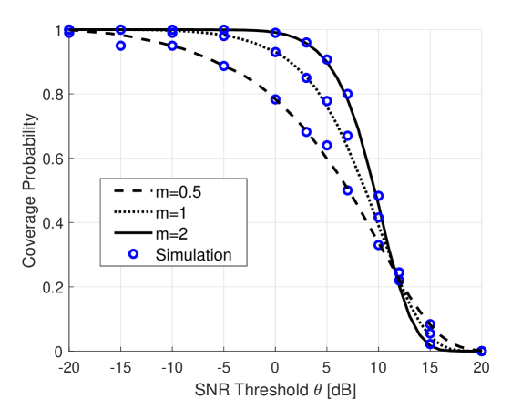
Figure 2: Coverage probability as a function of SNR threshold $\theta$ for $N=500$ reflecting antenna elements, $\alpha=4$, $\theta=5$ dB, $d=100$ m, $r=500$ m, $P=2.5$ W.

IV-3 Coverage as a function of number of IRS Elements

Fig. 3 illustrates the coverage probability $\mathcal{C}_{S}$ of the typical user as a function of finite number of IRS elements and distance from the IRS. We can see that by increasing the distance from the IRS and lower number of IRS elements, the coverage of the typical user significantly decreases. The IRS link is beneficial for small values of distance $d$ between the user and the IRS. In particular, for large values of $d$, the coverage from IRS link is nearly zero and the achieved 60% coverage can be observed only due to the direct link which is independent of the distance between the UE and the IRS.

Most of the existing research works considered asymptotically large numbers of IRS elements and relied on CLT, which may not yield accurate results. The reason is that an IRS surface is typically of a finite size and thereby possesses a finite number of IRS elements in practice. Fig. 3 offers insights related to the impact of a finite number of IRS elements on the coverage probability. This numerical result quantifies the performance gap considering both finite and infinite number of IRS elements (as illustrated by the difference in the coverage probability when $N=10$ and when $N=500$) and signifies the importance of exact coverage analysis.

Figure 3: Coverage probability as a function of the IRS elements $N$ when $m=0.5$, $\alpha=4$, $\theta=5$dB, $r=500$ m, $p=2.5$ W (The blue data points are obtained from analysis. The dotted black lines are obtained from simulations).

IV-4 Coverage probability as a function of the user’s distance from the IRS

Fig. 4 illustrates the coverage probability as a function of the user’s distance from the IRS and offers insights related to the benefits of IRS-aided transmissions over the direct link. In particular, the graph provides a comparative analysis of three modes of operation, 1) direct transmission, 2) IRS-aided transmission, and 3) IRS-aided transmission with direct link. We highlight points A and B in Fig. 4 where operations modes can be switched in order to enhance coverage probability. Furthermore, we note that the IRS link is beneficial for small values of distance $d$ between the user and the IRS. The graph in Fig. 4 indicates the maximum coverage distance of the IRS. That is, in the absence of a direct link, a user can choose the IRS if its distance is less than 30 m from the IRS equipped with 500 elements. If the direct link is available, it is beneficial to combine both signals up to a distance of 70 m. On the other hand, if the IRS is equipped with 100 elements, the user can choose the IRS if its distance is less than 20 m. If the direct link is available, it is beneficial to combine both signals up to a distance of 40 m. Our closed-form result given in Lemma 3 and numerical result in Fig. 4 provide visualization of the maximum coverage range of a given IRS and thus can be a useful tool for interference evaluation in large-scale networks.

Figure 4: Comparison of the coverage probability as a function of the user’s distance from the IRS, $m=0.5$.

IV-5 Channel hardening

In order to show the effect of channel hardening, in Fig. 5, we plot $\kappa$ as a function of the number of reflecting antenna elements $N$. As we can see in Fig. 5, given a value $N$, as $m$ increases (fading decreases), the channel hardening factor $\kappa$ also increases. Channel hardening correlates with a nearly deterministic channel with improved reliability, and requires less frequent channel estimation.

Figure 5: $\kappa$ as a function of number of reflecting antenna elements $N$ for different values of $m$.

V Conclusion

We characterize the coverage probability of IRS-aided communication networks with Nakagami-m channels, taking into account the direct link between the BS and UE in our model. The results reveal that the number of intelligent reflecting surfaces $N$ has a significant impact on the system performance, and that the use of IRSs enhances coverage for edge users. Our results show that the assumption of asymptotically large numbers of IRS in most of existing work can overestimate the users’ coverage probability compared to the exact users’ coverage probability. We provide a comparative analysis of three important IRS system modes of operation, 1) direct transmission, 2) IRS-aided transmission, and 3) IRS-aided transmission with direct link. We highlight points where modes have to be switched to achieve better coverage probability. Moreover, increasing the number of intelligent reflecting surfaces $N$ and reducing the fading severity (i.e., increasing the fading severity parameter) enhances the channel hardening in IRS-aided communication networks. Finally, we propose a closed-form expression to characterize the IRS coverage range for any network parameters.

References

- [1] M. Di Renzo, M. Debbah, D.-T. Phan-Huy, A. Zappone, M.-S. Alouini, C. Yuen, V. Sciancalepore, G. C. Alexandropoulos, J. Hoydis, H. Gacanin et al., “Smart radio environments empowered by reconfigurable AI meta-surfaces: An idea whose time has come,” EURASIP Journal on Wireless Communications and Networking, vol. 2019, no. 1, pp. 1–20, 2019.
- [2] E. Basar, M. Di Renzo, J. De Rosny, M. Debbah, M.-S. Alouini, and R. Zhang, “Wireless communications through reconfigurable intelligent surfaces,” IEEE Access, vol. 7, pp. 116 753–116 773, 2019.
- [3] C. Liaskos, S. Nie, A. Tsioliaridou, A. Pitsillides, S. Ioannidis, and I. Akyildiz, “A new wireless communication paradigm through software-controlled metasurfaces,” IEEE Communications Magazine, vol. 56, no. 9, pp. 162–169, 2018.
- [4] L. Yang, Y. Yang, M. O. Hasna, and M.-S. Alouini, “Coverage, probability of SNR gain, and DOR analysis of RIS-aided communication systems,” IEEE Wireless Communications Letters, 2020.
- [5] C. Zhang, W. Yi, Y. Liu, Z. Qin, and K. K. Chai, “Downlink analysis for reconfigurable intelligent surfaces aided NOMA networks,” arXiv preprint arXiv:2006.13260, 2020.
- [6] X. Yue and Y. Liu, “Performance analysis of intelligent reflecting surface assisted NOMA networks,” arXiv preprint arXiv:2002.09907, 2020.
- [7] M. H. Samuh and A. M. Salhab, “Performance analysis of reconfigurable intelligent surfaces over Nakagami-m fading channels,” arXiv preprint arXiv:2010.07841, 2020.
- [8] I. Trigui, W. Ajib, and W.-P. Zhu, “A comprehensive study of reconfigurable intelligent surfaces in generalized fading,” arXiv preprint arXiv:2004.02922, 2020.
- [9] R. C. Ferreira, M. S. Facina, F. A. De Figueiredo, G. Fraidenraich, and E. R. De Lima, “Bit error probability for large intelligent surfaces under double-nakagami fading channels,” IEEE Open Journal of the Communications Society, vol. 1, pp. 750–759, 2020.
- [10] P. K. Sharmay and P. Garg, “Intelligent reflecting surfaces to achieve the full-duplex wireless communication,” IEEE Communications Letters, 2020.
- [11] J. Lyu and R. Zhang, “Spatial throughput characterization for intelligent reflecting surface aided multiuser system,” IEEE Wireless Communications Letters, 2020.
- [12] Q. Wu and R. Zhang, “Towards smart and reconfigurable environment: Intelligent reflecting surface aided wireless network,” IEEE Communications Magazine, vol. 58, no. 1, pp. 106–112, 2019.
- [13] T. Shafique, H. Tabassum, and E. Hossain, “Optimization of wireless relaying with flexible UAV-borne reflecting surfaces,” IEEE Transactions on Communications, 2020.
- [14] Q. Wu and R. Zhang, “Intelligent reflecting surface enhanced wireless network via joint active and passive beamforming,” IEEE Transactions on Wireless Communications, vol. 18, no. 11, pp. 5394–5409, 2019.
- [15] G. K. Karagiannidis, N. C. Sagias, and T. Mathiopoulos, “The N* nakagami fading channel model,” in 2005 2nd International Symposium on Wireless Communication Systems. IEEE, 2005, pp. 185–189.
- [16] J. Gil-Pelaez, “Note on the inversion theorem,” Biometrika, vol. 38, no. 3-4, pp. 481–482, 1951.
- [17] A. Jeffrey and D. Zwillinger, Table of integrals, series, and products. Elsevier, 2007.
- [18] G. K. Karagiannidis, N. C. Sagias, and T. A. Tsiftsis, “Closed-form statistics for the sum of squared nakagami-m variates and its applications,” IEEE Transactions on Communications, vol. 54, no. 8, pp. 1353–1359, 2006.
- [19] H. Ibrahim, H. Tabassum, and U. T. Nguyen, “The meta distributions of the SIR/SNR and data rate in coexisting sub-6GHz and millimeter-wave cellular networks,” IEEE Open Journal of the Communications Society, vol. 1, pp. 1213–1229, 2020.
- [20] ——, “Meta distribution of SIR in dual-hop Internet-of-Things (IoT) networks,” in ICC 2019-2019 IEEE International Conference on Communications (ICC). IEEE, 2019, pp. 1–7.