CSIS: compressed sensing-based enhanced-embedding capacity image steganography scheme

Abstract

Image steganography plays a vital role in securing secret data by embedding it in the cover images. Usually, these images are communicated in a compressed format. Existing techniques achieve this but have low embedding capacity. Enhancing this capacity causes a deterioration in the visual quality of the stego-image. Hence, our goal here is to enhance the embedding capacity while preserving the visual quality of the stego-image. We also intend to ensure that our scheme is resistant to steganalysis attacks.

This paper proposes a Compressed Sensing Image Steganography (CSIS) scheme to achieve our goal while embedding binary data in images. The novelty of our scheme is the combination of three components in attaining the above-listed goals. First, we use compressed sensing to sparsify cover image block-wise, obtain its linear measurements, and then uniquely select permissible measurements. Further, before embedding the secret data, we encrypt it using the Data Encryption Standard (DES) algorithm, and finally, we embed two bits of encrypted data into each permissible measurement. This is the first attempt to rigorously embed more than one bit. Second, we propose a novel data extraction technique, which is lossless and completely recovers our secret data. Third, for the reconstruction of the stego-image, we use the least absolute shrinkage and selection operator (LASSO) for the resultant optimization problem. This has the advantages of fast convergence and easy implementation. This component is also new.

We perform experiments on several standard grayscale images and a color image, and evaluate embedding capacity, Peak Signal-to-Noise Ratio (PSNR) value, mean Structural Similarity (SSIM) index, Normalized Cross-Correlation (NCC) coefficients, and entropy. We achieve 1.53 times more embedding capacity as compared to the most recent scheme. We obtain an average of 37.92 dB PSNR value, and average values close to $1$ for both the mean SSIM index and the NCC coefficients, which are considered good. Moreover, the entropy of cover images and their corresponding stego-images are nearly the same. These assessment metrics show that CSIS substantially outperforms existing similar steganography schemes.

1 Introduction

The primary concern during the transmission of digital data over communication media is that anybody can access this data. Hence, to protect this data from being accessed by illegitimate users, the sender must employ some security mechanisms. In general, there are two main approaches used to protect secret data; cryptography Stalling and steganography Abbas . In cryptography, the encryption process transforms the secret data, known as plain-text, into cipher-text using an encryption key. This text is in unreadable form, hence, it attracts the opponents to exploit the content of the cipher-text by employing some brute-force attacks Stalling . However, steganography avoids this scenario.

Steganography is derived from the Greek words steganos means “covered or secret" and graphie means “writing". In steganography, the secret data is hidden into some other unsuspected cover media so that it is visually imperceptible. Here, both the secret data as well as the cover media may be text or multimedia. The media obtain after embedding secret data into cover media is called stego-media. Some recent steganography schemes that use text as cover media are MMT_2020 and Mathematics_2020 . In MMT_2020 , the authors have proposed an Arabic text steganography scheme, where the secret message is hidden within the text by using Unicode standard encoding. In Mathematics_2020 , the authors have proposed a character-level text generation-based linguistic steganography scheme, where the secret message is embedded in the text's content.

Recently, the steganography schemes that use images as the cover media have gained a lot of research interest due to their heavy use in Internet-based applications Typically, these images are transmitted in a compressed format. So here, we focus on compressed domain-based image steganography. In this, the challenges are;

1. Improving the embedding capacity.

2. Maintaining the quality of the stego-image.

3. The scheme should be resistant to steganographic attacks.

Although images can be embedded into images, our focus is on embedding binary data into images.

In the following paragraphs, first we discuss the way in which secret data can be embedded into cover images, then we summarize some existing schemes and their limitations, and finally we argue how the scheme presented in this paper outperforms the existing schemes.

Secret data can be embedded in images by two ways; spatially and by using a transform. In the spatial domain based image steganography scheme, secret data is embedded directly into the image by some modification in the values of the image pixels. Some well-known schemes here are listed in Abbas ; Chan1 ; Steg_2019_FGT ; Intech_2016 ; Intech2_2016 ; IEEE_2016 ; JIS_2018 ; Arabian_3D_Mesh_2018 . In the transform domain based image steganography scheme, first, the image is transformed into frequency components, and then the secret data is embedded into these components. Some commonly used such schemes are JSteg Jsteg , F5 F5 , and Outguess Outguess . Some other techniques, which do not carry specific names are given in references Chang ; Liu ; Pan ; Steg_ExpertSystem ; Steg_Rohit ; JAIS_2017 ; Elsvier_2018 ; IEEE_2019 ; Rohit_arXiv .

The spatial domain based image steganography outperforms the transform domain one in terms of embedding capacity, but the stego-image has a high amount of redundant data. Digital images transmitted through communication media are usually of this type. Since transform based schemes reduce the redundancy present in the image and represent it in a compressed form, they are preferred for transmission.

Most of the transform domain based scheme follow either Discrete Cosine Transform (DCT) or Wavelet Transform (WT). The DCT based schemes are also called the JPEG compression based image steganography techniques. Several variants of DCT based schemes have been proposed in the literature Jsteg ; F5 ; Outguess ; Chang ; Liu ; Pan ; Steg_Rohit ; JAIS_2017 ; Elsvier_2018 ; IEEE_2019 ; Rohit_arXiv . For the schemes Jsteg ; F5 ; Outguess ; Chang ; Liu ; Pan ; Steg_Rohit ; Elsvier_2018 ; IEEE_2019 , secret data is binary bits, and for JAIS_2017 ; Rohit_arXiv , secret data is images.

In Jsteg ; Outguess ; Chang , the secret data is embedded by flipping the least significant bit (LSB) of the quantized DCT coefficients obtained from the cover image. This process is considered as a direct embedding mechanism. Alternatively, methods in F5 ; Liu ; Pan ; Steg_Rohit ; Elsvier_2018 ; IEEE_2019 ; JAIS_2017 ; Rohit_arXiv are considered as indirect steganography schemes in which the quantized DCT coefficient values are altered according to certain secret message bits or secret image pixels. By steganalysis, which is the study of detecting the secret data hidden using steganography, it has been observed that the indirect steganography mechanism is superior to the direct one due to its capability in resisting certain statistical attacks. The most common statistical attacks are the chi-square test, and the shrinkage effect Westfeld ; Fridrich ; Patsakis . Hence, the schemes Jsteg ; Outguess ; Chang are not resistant to such attacks, while the schemes F5 ; Liu ; Pan ; Steg_Rohit ; Elsvier_2018 ; IEEE_2019 ; JAIS_2017 are resistant to them, but their embedding capacity is limited. If we try to increase the embedding capacity of the later schemes, then the quality of the stego-images gets degraded. The scheme Rohit_arXiv has high embedding capacity with resistance to steganographic attacks, but here, the secret data is the images, which is different from our goal of embedding binary data in images.

Most recent Wavelet transform based steganography schemes are given in Steg_ExpertSystem ; DWT_2019 . In Steg_ExpertSystem , the authors have proposed a steganography scheme based upon edge identification and XOR coding that uses Wavelet transformation. This scheme is resistant to steganographic attacks, but here also the embedding capacity is significantly less. As above, if we try to increase embedding capacity, then the quality of stego-image gets degraded. The scheme given in DWT_2019 embeds a medical image into a cover image using Redundant Integer Wavelet Transform (RIWT) and DCT. This scheme's purpose is again different from ours of embedding binary data in images.

As discussed above, conventional transform domain based image steganography schemes provide good visual quality stego-image and are resistant to steganographic attacks, but their embedding capacity is limited. If we try to increase their embedding capacity, then the stego-image quality degrades. To overcome this limitation, in this manuscript, we utilize another paradigm, the compressed sensing, which also fulfills all the requirements of image steganography. Next, we present literature regarding compressed sensing-based steganography schemes. These works help to achieve some of the above objectives of steganography but not all, which we do.

In Sreedhanya , and Rohit , steganography schemes based on compressed sensing and Singular Value Decomposition (SVD) have been presented. In these schemes, secret medical image data is embedded into an image cover media. Both these approaches use a similar embedding approach, but use compressed sensing differently. In these, first, encrypted measurements of the secret image are obtained using the compressed sensing technique, and then these encrypted measurements are embedded into the cover image using SVD based embedding algorithm. In Sreedhanya , the PSNR (Peak Signal-to-Noise Ratio, discussed in Section 4.2.2) value of the stego-image is greater than 30 dB, which shows that it produces good quality stego-images. But the PSNR value of the constructed secret image is very low, i.e. the quality of the secret image is degraded very much. In contrast, in Rohit , both the stego-image as well as the reconstructed secret image preserved good visual quality. But, the goal in both these schemes is different from ours. In these schemes, the secret data is an image. If these techniques are applied on binary data that we want to embed, the information will be lost. In Pan , the authors have proposed an image steganography scheme based on sub-sampling and compressed sensing. In this scheme, the PSNR value of the stego-image is greater than 30 dB, also the secret data is binary. However, the embedding capacity in this scheme is very low.

Moreover, some other compressed sensing-based image steganography schemes are listed in Patsakis , Patsakis1 , and MMT_2019 . In Patsakis , the authors have presented the application of compressed sensing to detect steganographic content in the LSB steganography scheme. In Patsakis1 , the authors have proposed a DCT steganography classifier based on a compressed sensing technique. Here, the original image is identified from a set of images containing the original image and some instances of stego images. In MMT_2019 , the authors have proposed an image steganalysis technique for secret signal recovery. These steganography schemes are not related to our work because the focus of Patsakis and MMT_2019 is steganalysis, while Patsakis1 focuses on steganography classifier. Hence, we do not discuss these schemes in detail.

The scheme that we propose satisfies all the goals mentioned in the earlier paragraphs, i.e. increased embedding capacity without degrading the quality of stego-images as well as making the scheme resistant to steganalysis attacks. Our scheme has three components, which we discussed next. The first component of our scheme consists of three parts; (1) we use compressed sensing to sparsify cover image block-wise and obtain linear measurements. Here, we design an adaptive measurement matrix instead of using a random one. Using our adaptive measurement matrix, we uniquely select a large number of permissible measurements compared to existing schemes. Hence, we achieve a high embedding capacity. Moreover, these measurements act as encoded transformed coefficients, and hence, this adds security to our proposed scheme as well; (2) we encrypt the secret data using the Data Encryption Standard (DES) algorithm Stalling . This adds another layer of security to our scheme; (3) we embed two bits of secret data into each permissible measurement instead of commonly embedding one bit per measurement. This is a first attemp to rigorously embed more than one bit. Second, we completely extract secret data without any loss using our extraction algorithm. Third, we use the alternating direction method of multipliers (ADMM) solution of the least absolute shrinkage and selection operator (LASSO) formulation of the underlined optimization problem in the stego-image construction. The advantages of using ADMM and LASSO are that they have broad applicability in the domain of image processing, require a little assumption on the objective function's property, have fast convergence, and are easy to implement. This is also a completely new contribution.

For performance evaluation, we perform experiments on standard test images. To check the quality of stego-image, we reconstruct it from the obtained modified measurements and then compare it with its corresponding cover image. We evaluate embedding capacity, Peak Signal-to-Noise Ratio (PSNR) value, mean Structural Similarity (SSIM) index, Normalized Cross-Correlation (NCC) coefficient, and entropy. We achieve 1.53 times more embedding capacity when compared with the most recent scheme of this category. We achieve a maximum of 40.86 dB and an average of 37.92 dB PSNR values, which are considered good. The average values of mean SSIM index and NCC coefficients are close to 1, which are again considered good. Moreover, the entropy of cover images and their corresponding stego-images are nearly the same. In the Experimental Results section, we also show that our scheme outperforms existing compression based steganography schemes Jsteg ; F5 ; Outguess ; Liu ; Pan ; Steg_Rohit ; Steg_2019_FGT ; Steg_ExpertSystem .

The rest of the paper has four more sections. Section 2 describes the compressed sensing technique. Section 3 explains our proposed steganography scheme including embedding of the data, extracting it, and stego-image reconstruction process. Section 4 presents the experimental results. Finally, Section 5 gives conclusions and future work.

2 Compressed Sensing

Compressed sensing is used to acquire and reconstruct the signal efficiently. Traditionally, the successful reconstruction of the signal from the measured signal must follow the popular Nyquist/ Shannon sampling theorem, which states that the sampling rate must be at least twice the signal bandwidth. In many applications such as image, audio, video, data mining, and wireless communications & networks, where the signal is sparse or sparsified in some domain, the Nyquist rate is too high to achieve. There is a fairly new paradigm, called compressed sensing that can represent the sparse signal by using a sampling rate significantly lower than the Nyquist sampling rate Candes ; Donoho . Hence, the application of compressed sensing has gained popularity in many areas. Some of them are image processing Romberg , radar system Steeghs , MRI Imaging CS_MRI , and noise separation from data Romberg .

Compressed sensing projects the sparse signal onto a small number of linear measurements in such a way that the structure of this signal remains the same. The sparse signal can be reconstructed approximately from these measurements by an optimization technique. However, the reconstruction of the signal is possible only when the original signal is sparse, and it satisfies the Restricted Isometric Property (RIP) Candes2 (discussed in Section 2.2). If the original signal is not sparse, then it can often be artificially sparsified. A brief description of signal sparsification, obtaining linear measurements, and reconstruction of the approximate sparse signal is given next.

2.1 Signal Sparsification

Let the original signal be $x\in\mathbb{R}^{N\times 1}$. The signal x is K sparse when it has maximum K number of non-zeros coefficients, i.e. $\left\|x\right\|_{0}\leq K$, where $||\cdot||_{0}$ denotes the $\ell_{0}-norm$ of a vector, and the remaining coefficients are zero or nearly zero. Let the original signal x not be sparse and be represented in-terms of $\left\{\psi_{i}\right\}_{i=1}^{N}$ basis vectors each of length $N\times 1$, then

$$s=\Psi^{T}x,$$ (1)

where, $s\in\mathbb{R}^{N\times 1}$ and $\Psi=\left[\psi_{1},\psi_{2},...,\psi_{N}\right]\in\mathbb{R}^{N\times N}$ is an orthogonal matrix. If $K\ll N$ then this signal is sparsifiable Candes3 , $s$ is the sparse representation of $x$, and $\Psi$ is the corresponding sparsification matrix.

2.2 Sensing Matrix and Linear Measurements

In the compressed sensing framework, we acquire $M(M<N)$ linear measurements from the inner product between the original signal $x\in\mathbb{R}^{N\times 1}$ and M measurement vectors $\left\{\phi_{i}\right\}_{i=1}^{M}$, where $\phi_{i}\in\mathbb{R}^{N\times 1}$. Considering the measurement/ sensing matrix as $\Phi=\left[\phi_{1}^{T};\phi_{2}^{T};...;\phi_{M}^{T}\right]\in\mathbb{R}^{M\times N}$, the measurements $y\in\mathbb{R}^{M\times 1}$ are given as Candes3

$$y=\Phi x.$$ (2)

If the input signal is not sparse but sparsifiable, then using the above theory we get

$$y=\Phi\Psi s=\Theta s,$$ (3)

where $\Theta=\Phi\Psi$ is again the measurement matrix of size $M\times N$. Usually, in the compressed sensing framework, the measurement matrix is nonadaptive. That is, the measurement matrix is fixed and does not depend on the signal. However, in certain cases, adaptive measurements can lead to significant performance improvement.

The main concern here is to design the measurement matrix in such a way so that the most of the information and the structure of the signal is preserved in the measurements. This would imply that original signal would be recovered efficiently from these measurements. To achieve this, for all K-sparse signals $s$, the measurement matrix should hold the following inequality Candes2 .

$$\left(1-\delta_{K}\right)\leq\frac{\left\|\Theta s\right\|_{2}^{2}}{\left\|s\right\|_{2}^{2}}\leq\left(1+\delta_{K}\right),$$ (4)

where $\delta_{K}\in(0,1)$ is an isometric constant. The above inequality is called the RIP that informally says that the $\ell 2-norm$ of the sparse signal $s$ and the measurement $\Theta s$ should be comparable. Apart from satisfying the RIP, the minimum number of measurements required, i.e. the minimum value of $M$, is also a concern in the measurement matrix design.

2.3 Reconstruction of the Approximate Signal

As discussed in the previous subsection, size of the measurement $y=\Phi x=\Phi\Psi s=\Theta s$ is less than the size of the original signal $s$. Hence, the reconstruction of the signal from measurements becomes an ill-posed problem. That is, the solution of an under-determined linear system of equations is to be found. If the matrix $\Theta$ satisfies the RIP, then the sparse signal $s$ can be reconstructed approximately by solving the following optimization problem Baraniuk :

$$\min_{s}\left\{\text{number of i such that}\>s\left(i\right)\neq 0\right\}$$ (5)

$$\text{Subject to}\hskip 2.84544pt\Phi\Psi s=y.$$

In the above equation, the function to be minimized is simply the number of nonzero coefficients in the vector $s$. This equation is referred to as $\ell_{0}-norm$ minimization problem. It is combinatorial and an NP-hard problem Baraniuk . The other approach is to substitute the $\ell_{0}-norm$ by the closest convex norm, i.e. the $\ell_{1}-norm$, or

$$\min_{s}\left\|s\right\|_{1}$$ (6)

$$\text{Subject to}\hskip 2.84544pt\Phi\Psi s=y,$$

where $||\cdot||_{1}$ denotes the $\ell_{1}-norm$ of a vector. The approach to reconstruct the sparse signal $s$ by solving the above equation is termed as a convex optimization method.

Other approaches such as Greedy based (OMP OMP , CoSaMP Needell ), sparse reconstruction by separable approximation Stephen , Bayesian strategy David , and ADMM solution of the LASSO formulation of the above optimization problem can also be used to reconstruct the sparse signal from the measurements ADMMSBoyd ; Lasso .

Next, we give a brief idea of LASSO and ADMM, which we use. The general LASSO problem is given as Lasso

$$\min_{z}\left\{\frac{1}{2}\|Az-b\|_{2}^{2}+\lambda\|z\|_{1}\right\},$$ (7)

where $z\in\mathbb{R}^{n}$, $A\in\mathbb{R}^{p\times n}$, $b\in\mathbb{R}^{p}$, $\|\cdot\|_{2}$ is the $\ell_{2}$ norm and $\lambda>0$ is a scalar regularization parameter also called Lagrangian parameter ParaLarPD . Further, (7) is transformed into a form solvable by ADMM ADMMSBoyd . That is

$$\begin{split}&\min\limits_{z,z_{1}}\left\{\frac{1}{2}\|Az-b\|_{2}^{2}+\lambda\|z_{1}\|_{1}\right\}\\ &\text{ Subject to }z-z_{1}=0.\end{split}$$ (8)

Finally, ADMM solve the above optimization problem.

Now, we discuss how to solve our signal reconstruction problem, i.e. (LABEL:eq:_CS_reconstruction_l1) by LASSO and ADMM. For our case, $\Theta=\Phi\Psi$ is the measurement matrix, and $\Theta\in\mathbb{R}^{M\times N}$. In the compressed sensing framework, matrix $\Theta$ is underdetermined, i.e. $M<N$. Hence, there is equivalent solution of (LABEL:eq:_CS_reconstruction_l1), which is given as l1_Lasso

$$\min_{s}\left\{\frac{1}{2}\left\|\Theta s-y\right\|_{2}^{2}+\lambda\left\|s\right\|_{1}\right\}$$ (9)

Here, we observe that (LABEL:eq:_CS_reconstruction_Lasso) is equivalent to (7) with $\Theta=A$, $s=z$ and $y=b$.

Finaly, we briefly mention a theoretical result related to reconstruction. In Candes4 , it is shown that for sufficiently small constant C ($C>0$), the K-sparse signal $s$ of size N can be approximately reconstructed from M measurements $y$ if $M\geq CK\left(\log N\right)$. After recovering the sparse signal $s$, the original signal $x$ can be obtained as $x=\Psi s$. For us, this property holds.

3 Proposed Method

Our proposed compressed sensing-based image steganography scheme consists of the following components; data embedding, data extraction, and stego-image construction, which are discussed in the respective sections below.

Algorithm 1 Embedding Rule

1: 

• $y$: Sequence of transform coefficients.

• S: Encrypted secret bit sequences which is to be embedded.

2: 

• $z$: The modified version of transform coefficients.

3:if ($length(S)<2\times length(y)$) then

4:    for $j=1$ to $length(y)$ do

5:       if (${y}\left(j\right)=-1$ or ${y}\left(j\right)=0$ or ${y}\left(j\right)=+1$) then

6:          ${z}={y}$  (Do not embed in these measurements)

7:       else

8:          if (${y}\left(j\right)\%2=0$) then

9:             if (${y}\left(j\right)\%4=0$) then

10:                if ($S\left(j\right)=00$) then

11:                   ${z}={y}+1$

12:                else if ($S\left(j\right)=01$) then

13:                   ${z}={y}$

14:                else if ($S\left(j\right)=10$) then

15:                   ${z}={y}-1$

16:                else if ($S\left(j\right)=11$) then

17:                   ${z}={y}+2$ or ${z}={y}-2$

18:                end if

19:             else

20:                if ($S\left(j\right)=00$) then

21:                   if (${y}\neq 2$) then

22:                      ${z}={y}-1$

23:                   else

24:                      ${z}={y}+3$

25:                   end if

26:                else if ($S\left(j\right)=01$) then

27:                   if (${y}\neq-2$) then

28:                      ${z}={y}+2$

29:                   else

30:                      ${z}={y}-2$

31:                   end if

32:                else if ($S\left(j\right)=10$) then

33:                   if (${y}\neq-2$) then

34:                      ${z}={y}+1$

35:                   else

36:                      ${z}={y}-3$

37:                   end if

38:                else if ($S\left(j\right)=11$) then

39:                   ${z}={y}$

40:                end if

41:             end if

42:          else

43:             if ((${y}\left(j\right)-1)\%4=0$) then

44:                if ($S\left(j\right)=00$) then

45:                   ${z}={y}$

46:                else if ($S\left(j\right)=01$) then

47:                   ${z}={y}-1$

48:                else if ($S\left(j\right)=10$) then

49:                   ${z}={y}-2$

50:                else if ($S\left(j\right)=11$) then

51:                   ${z}={y}+1$

52:                end if

53:             else

54:                if ($S\left(j\right)=00$) then

55:                   ${z}={y}+2$

56:                else if ($S\left(j\right)=01$) then

57:                   ${z}={y}+1$

58:                else if ($S\left(j\right)=10$) then

59:                   ${z}={y}$

60:                else if ($S\left(j\right)=11$) then

61:                   ${z}={y}-1$

62:                end if

63:             end if

64:          end if

65:       end if

66:    end for

67:else

68:    Whole secret data cannot be embedded. Try short length secret data.

69:end if

70:return $z$

3.1 Data Embedding

Figure 1: The Embedding Process

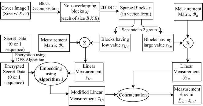
The first step in any compressed sensing-based image steganography scheme is the input image's sparsification if it is not sparse at the start. This step is equivalent to the signal sparsification of Section 2.1. Methods such as K-SVD, DCT, Discrete Walsh Transform, Stationary Wavelet Transform, and Discrete Rajan Transform provide good sparsification. Since the distortion due to DCT is less, we use it as our sparsifying agent. To further reduce the distortion, instead of sparsifying the whole image at once, first, we decompose the cover image into non-overlapping blocks of the same size, and then each block is sparsified.

Let the image I's size be $r1\times r2$ and each block size be $B\times B$, then we have $(r1\times r2)/B^{2}$ number of blocks. In our case, $r1=r2$ and $B$ completely divides $r1$. The block-wise sparsification is now done as

$$s_{i}=DCT\left(x_{i}\right),$$ (10)

where $i=1,2,\cdots,(r1\times r2)/B^{2}$, $x_{i}$ and $s_{i}$ are the $i^{th}$ original and sparse blocks of the same size, i.e. $B\times B$, respectively. Next, we convert each block into their vector representation by stacking them column-wise. Thus, $s_{i}$ becomes a vector of size $B^{2}\times 1$. Because of sparsification, each sparse vector has few coefficients of large values and the remaining coefficients of very small values or zero. Hence, we categories each vector into two groups. Let $p_{1}$ be the number of coefficients having large values and $p_{2}$ be the number of coefficients having small values or zero values. Note that here, $p_{1}<p_{2}$ as each of these vectors are sparse in nature and $p_{1}+p_{2}=B^{2}$. We represent each vector in two groups based upon these coefficients, i.e. $s_{i,u}\in\mathbb{R}^{p_{1}}$ and $s_{i,v}\in\mathbb{R}^{p_{2}}$. Now, we project each sparse vector onto linear measurements using a measurement matrix, which is equivalent to Section 2.2.

There are two ways to choose the measurement matrix: either randomly or deterministically. Randomly generated matrices such as the Independent and Identically Distributed (i.i.d.) Gaussian matrix, the Bernoulli matrix or other matrices generated by probabilistic methods are nonadaptive, although they satisfy the RIP. Deterministically generated matrices are the ones that are designed such that specific properties are satisfied, e.g., adaptiveness and the RIP. We design a deterministic matrix that is adaptive to our sparse vector since this improves the efficiency of compressed sensing. To achieve RIP here, the projected linear measurements are enforced to have almost the same $\ell_{2}-norm$ as that of the sparse vector.

One way to design the measurement matrix is to first analyze the distribution of all $B^{2}$ coefficients in each sparse vector, and then find the $m$ indices out of these that give maximum $\ell_{2}-norm$ Xiaorong . That is ,

$$E_{max}^{|m|}=\max_{i\in m\subset B^{2}}\left\|s_{i}\right\|_{2}^{2},$$ (11)

where $|m|$ is the number of entries in set $m$ and $E_{max}^{|m|}$ is a variable that stores the maximum value of square of $\ell_{2}$-norm of vector $s_{i}$ for $i\in m\subset B^{2}$. However, in this paper, we use the property of DCT to design the measurement matrix. This property states that DCT coefficients can be divided into three sets; low frequency, middle frequency, and high frequency components. Low frequency corresponds to the overall image information, middle frequency corresponds to the structure of the image, and high frequency corresponds to the noise or small variance. For image reconstruction, only lower and middle frequency components are useful. Hence, we select $m$ indices out of all $B^{2}$ indices that correspond to these two sets of frequency Chang . Here, $|m|$ is a user-defined parameter such that $p_{1}<|m|<p_{1}+p_{2}$, and is discussed in Experimental Results section. As discussed earlier, in this subsection we have two groups of sparse vectors $s_{i,u}$ and $s_{i,v}$. Hence, we design two different measurement matrices $\Phi_{u}$ and $\Phi_{v}$ corresponding to $s_{i,u}$ and $s_{i,v}$, respectively.

Since $\left\|s_{i,u}\right\|_{2}$ is close to $\left\|s_{i}\right\|_{2}$ because $s_{i,u}$ contains large value coefficients of $s_{i}$, we project $s_{i,u}$ onto the same number of linear measurements. Thus, we have $\Phi_{u}=\alpha I_{p_{1}}$, where $I_{p_{1}}$ is the identity matrix of size $p_{1}\times p_{1}$, and $\alpha$ is a small constant.

As mentioned in Section 2.2, the main purpose of measurement matrix is to project the sparse vector onto less number of linear measurements. Hence, we project $s_{i,v}$ onto $|m|-p_{1}$ measurements or the size of $\Phi_{v}$ is $(|m|-p_{1})\times p_{2}$. To construct $\Phi_{v}$, we first take a random Hadamard matrix of size $p_{2}\times p_{2}$, which is a standard procedure in compressed sensing literature Hadamard , and then we choose $|m|-p_{1}$ rows from the available $p_{2}$ rows. These rows map to the last of $|m|-p_{1}$ indices from the index set $m$. This is because the first $p_{1}$ indices have the overall image information, and hence, map to construction of $\Phi_{u}$.

We use the same measurement matrices for all blocks. This is because, for all blocks of an image, the distribution of coefficients of the generated sparse vectors is almost the same. Thus, for each block $i=1,2,\dots,(r1\times r2)/B^{2}$, the block-wise linear measurements vector $y_{i}\in\mathbb{R}^{|m|}$ is given as

$$y_{i}=\begin{bmatrix}y_{i,u}\\ y_{i,v}\end{bmatrix}=\begin{bmatrix}\Phi_{u}s_{i,u}\\ \Phi_{v}s_{i,v}\end{bmatrix}.$$ (12)

Using the standard terminology Candes ; Donoho , the measurements $y_{i,u}$ are called the ordinary samples or non-compressed samples, and the measurements $y_{i,v}$ are called the compressed sensing samples.

Next, we discuss the encryption process of the secret data $D$ that is to be embedded. This data is a sequence of $0s$ and $1s$. As mentioned in the Introduction, this provides an extra layer of security to the embedded data. For this, we first encrypt this data by using DES algorithm to obtain the encrypted secret data $S$ (which is also a sequence of $0s$ and $1s$) Stalling . DES is a fairly standard algorithm used for data encryption Stalling . Then, we represent $S$ as a set of two-two bits, i.e. $S=\left\{S_{1},S_{2},\dots,S_{n}\right\}$, where each $S_{L}$ consists of two bits.

Next, we embed the secret data in our linear measurements $y_{i}$. The embedding rule is summarized in Algorithm 1, and helps to embed two bits into the transform coefficients. The rule is designed in such a way so that the secret data could be extracted without any loss, discussed in Data Extraction and Experimental Result sections. We embed the data in $y_{i,v}$ and not $y_{i,u}$. This is because $y_{i,u}$ corresponds to sparse vector coefficients of large values, and embedding in it leads to degradation of image quality. Further, in $y_{i,v}$, the secret data is embedded selectively. We do not embed in $y_{i,v}$ with measurement value of $-1$, $0$ and $1$. This is because our embedding algorithm concatenates the measurement values with integers from $-3$ to $+3$, and if these values are $-1$, $0$ or $1$, then we may end up getting many $0s$ after concatenation, which leads to difficulty in the extraction process. After embedding in other measurement values of $y_{i,v}$, we obtain the modified $y_{i,v}$, which is termed as $z_{i,v}$. That is,

$$z_{i,v}=\begin{cases}y_{i,v}&\text{if }y_{i,v}=-1,\>0\>or\>1\\ y_{i,v}+c&\text{otherwise},\end{cases}$$ (13)

where $c\in\{-3,-2,-1,0,1,2,3\}$. We obtain our stego-data by concatenating the measurements $y_{i,u}$ and $z_{i,v}$ as $\begin{bmatrix}y_{i,u}\\ z_{i,v}\end{bmatrix}$. The block diagram for this complete data embedding process is given in Fig. 1.

3.2 Data Extraction

In this section, we explain the process of extracting embedded secret data from our stego-data. The steps of this extraction process are given below, which are exactly reverse to our data embedding process.

1. Separate the measurements $z_{i,v}$ from the stego-data, i.e. $\begin{bmatrix}y_{i,u}\\ z_{i,v}\end{bmatrix}$, where $i=1,2,\dots,(r1\times r2)/B^{2}$ is the block number, and $u,v$ are indices available from the previous subsection.

2. Extract only those measurements from $z_{i,v}$ whose values are not equal to $-1$, $0$ or $1$. The embedding rule ensures that the embedded data could be extracted without loss. In other words, Algorithm 1 ensures that no secret data is embedded in measurements with values $-1$, $0$ and $1$.

3. Extract the encrypted message ${S}^{\prime}$ from the measurements obtained in the above step by applying Algorithm 2.

4. Decrypt this ${S}^{\prime}$ by DES algorithm, and obtain the extracted secret data $D^{\prime}$.

Figure 2: The Extraction Process

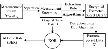
Now, we check the correctness of this extracted secret data $D^{\prime}$ by comparing it with original secret data $D$. For this, we use the Bit Error Rate (BER), which is given as Pan

$$\text{Error Bits (EB)}=D\bigoplus{D}^{\prime},$$ (14)

$$BER=\frac{\text{Number of ones in EB}}{\text{Size of D}}\times 100\%,$$ (15)

where $\bigoplus$ denotes the bitwise XOR/ Exclusive OR operation. The BER value for our steganography scheme is $0\%$, i.e. we successfully extract complete secret data without any error. This is the property of our embedding rule. The above extraction process is represented via a block diagram in Fig. 2.

Algorithm 2 Extraction Rule

1: 

• $z$: Sequence of modified linear measurements. These are $z_{i,v}$ that are not having value equal to $0$, $1$ or $-1$. See extraction process in Section 3.2.

2: 

• ${S}^{\prime}$: Encrypted secret bit sequences.

3:for $j=1$ to $length(z)$ do

4:    if (${y}\left(j\right)=-1$ or ${y}\left(j\right)=0$ or ${y}\left(j\right)=+1$) then

5:       Continue

6:    else

7:       if (${z}\left(j\right)\%2=0$) then

8:          if (${z}\left(j\right)\%4=0$) then

9:             ${S}^{\prime}\left(j\right)=01$

10:          else

11:             ${S}^{\prime}\left(j\right)=11$

12:          end if

13:       else

14:          if ((${z}\left(j\right)-1)\%4=0$) then

15:             ${S}^{\prime}\left(j\right)=00$

16:          else

17:             ${S}^{\prime}\left(j\right)=10$

18:          end if

19:       end if

20:    end if

21:end for

22:return ${S}^{\prime}$

3.3 Stego-Image Construction

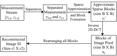
When the stego-data is transferred over a communication media, the intruder can access this data from the public channel and can try to construct the stego-image. If the intruder obtains a high visual quality image, then the goal of steganography is fulfilled. This is because he/ she will not be able to judge whether some data is hidden in the image or not. Therefore, in this subsection, we give the steps to construct the stego-image from the stego-data, which is equivalent to Section 2.3. We refer this process as construction rather than reconstruction.

1. Obtain the approximate sparse vector ${s}^{\prime}$ from the stego-data and measurement matrices $\Phi_{u}$ and $\Phi_{v}$ as (recall (12))

   $${s}^{\prime}_{i,u}=\Phi_{u}^{-1}y_{i,u},\>and$$ (16)

   $${s}^{\prime}_{i,v}=ADMM\_LASSO\left(z_{i,v},\Phi_{v}\right).$$

   Here, as discussed in Section 2.3, we use ADMM and LASSO to construct ${s}^{\prime}_{i,v}$. The sparse vector ${s}^{\prime}$ is obtained by concatenating ${s}^{\prime}_{i,u}$ and ${s}^{\prime}_{i,v}$. Here, the size of ${s}^{\prime}_{i,u}$, ${s}^{\prime}_{i,v}$, and ${s}^{\prime}$ is the same as that of $s_{i,u}$, $s_{i,v}$, and $s$, respectively.

2. Convert each vector ${s}^{\prime}_{i}$ into a block of size $B\times B$.

3. Apply two-dimensional Inverse DCT (IDCT) to each of these blocks to generate blocks ${x}^{\prime}_{i}$ of image. That is, recall (10),

   $${x}^{\prime}_{i}=IDCT\left({s}^{\prime}_{i}\right).$$ (17)

4. Construct the stego-image of size $r1\times r2$ by arranging all these blocks ${x}^{\prime}_{i}$.

The block representation of these steps is given in Fig. 3. We show in the Experimental Results section that image obtained from this stego-data preserves the quality of the original image.

Figure 3: Stego-Image Construction

As earlier, we term our proposed steganography scheme as Compressed-Sensing-Image-Steganography (CSIS) because we use compressed sensing to enhance the embedding capacity of the image steganography scheme.

4 Experimental Results

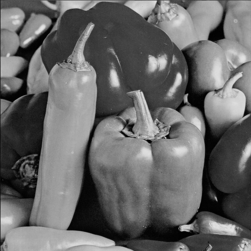
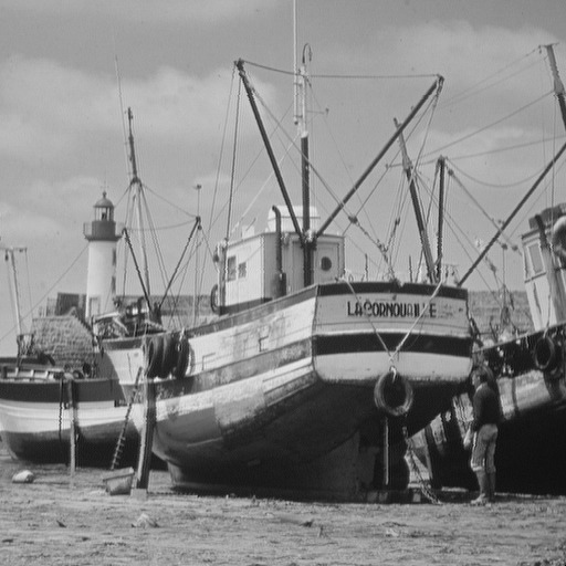
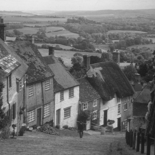
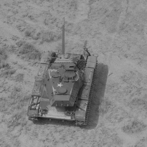
Experiments are carried out in MATLAB on a machine with an Intel Core i3 processor @2.30 GHz and 4GB RAM. We use a set of standard grayscale images to test our CSIS. Sample test images are shown in Fig. 4 and Fig. 5. These images have the varying texture property and are taken from the miscellaneous category of USC-SIPI image database SIPI and two other public domain databases ImageDatabase1 ; ImageDatabase2 .

The miscellaneous category of USC-SIPI database consists of 24 grayscale images. Some images, such as Lena, and Tiffany are no longer available in this database. These images have played a significant role in image processing, and literature. Thus, we use other public-domain test images databases ImageDatabase1 ; ImageDatabase2 for them. A total of seven such images are chosen. Hence, we have a total of 31 grayscale images. Our CSIS is also applicable to color images, and we pick one of them from USC-SIPI database.

In this manuscript, we report average values of all the 31 images with detailed results for 10 images due to space limitations. This is further justified by the fact that the image processing literature has used these 10 images or a subset of them.

The size of each of test images is $512\times 512$, i.e. $r1\times r2$. We take blocks of size $8\times 8$, i.e. $B\times B$. As earlier, the size of measurement matrix $\Phi_{u}$ is $p_{1}\times p_{1}$. Recall from Section 3.1, $p_{1}$ is the number of coefficients with large values/ low frequency in the input sparse vector. For commonly used images, this value is between $10$ and $14$ Chang ; NC . Since the measurement matrix cannot be different for every input matrix, we do experiments with three different values of $p_{1}$ ($10$, $12$ and $14$) to find the optimal one here. Again from Section 3.1, the size of measurement matrix $\Phi_{v}$ is $(|m|-p_{1})\times p_{2}$. We take $|m|$ from the following range Chang ; NC : $\{32,35,36,37,39,40,42,47\}$, and as before, $p_{2}=B\times B-p_{1}$ (i.e. $p_{2}=64-p_{1}$). For secret data, we use randomly generated data, which is sequence of $0$ and $1$ bits.

First, we check the embedding capacity of our proposed scheme. Second, we do the similarity analysis between the cover images and the constructed stego-images by assessing . Third, in the remainder of this section, we do security analysis, perform five comparisons with existing steganography schemes, and also experiment with a color image.

(a) Lena

(b) Peppers

(c) Boat

(d) Goldhill

(e) Zelda

Figure 4: Test images used in our experiments

(a) Tiffany

(b) Living room

(c) Tank

(d) Airplane

(e) Camera man

Figure 5: Continued from Fig. 4; test images used in our experiments

4.1 Embedding Capacity Analysis

Embedding capacity is defined as the maximum number of bits embedded in the cover media, which is the image here. The embedding capacity of our proposed steganography scheme depends on the sampling rate (SR), which is given as

$$SR=\frac{\text{Total Linear Measurements}}{\text{Total Pixels in Cover Image}}.$$ (18)

We have $r_{1}\times r_{2}$ total pixels in the cover image and $|m|$ linear measurements for each block with $\frac{r1\times r2}{B\times B}$ number of blocks. Therefore, our sampling rate is

$$SR=\left(\frac{|m|}{r1\times r2}\right)\times\left(\frac{r1\times r2}{B\times B}\right)=\frac{\left|m\right|}{B\times B}.$$ (19)

From this definition, it is evident that embedding capacity mainly depends upon $|m|$, however, the compressed image quality depends upon both $p_{1}$ and $|m|$. Therefore, to maintain the quality of stego-image while enhancing embedding capacity, the combination of these parameters is critical.

For different combinations of $p_{1}$ and $|m|$, in Table 4.1, we give the embedding capacity in bits of our proposed CSIS for the 10 test images of Fig. 4 and Fig. 5 and the average capacity for all the 31 images. We analyze the data of this table by comparing $p_{1}$ and $|m|-p_{1}$ instead of $p_{1}$ and $|m|$ because the former set directly maps to the number of ordinary samples and compressed sensing samples, respectively. When $p_{1}$ is constant, and $|m|-p_{1}$ is increased, the number of compressed sensing samples increases, where the secret data bits are embedded, leading to increased capacity. For example, consider columns $2$ and $3$ of Table 4.1, we can observe that the embedding capacity increases when $p_{1}$ is constant, i.e. $10$ and $|m|-p_{1}$ is increased from $22$ to $25$. When $|m|-p_{1}$ is constant and $p_{1}$ is increased, the number of compressed sensing samples decrease leading to decreased embedding capacity. For example, consider columns $3$ and $4$, we observe that embedding capacity decreases when $|m|-p_{1}$ is constant, i.e. $25$ and $p_{1}$ is increased from $10$ to $12$.

Embedding capacity (in bits) obtain by proposed CSIS for different parameters and for different test images Test image Parameters $p_{1}=10$ $|m|=32$ $p_{1}=10$ $|m|=35$ $p_{1}=12$ $|m|=37$ $p_{1}=12$ $|m|=40$ $p_{1}=12$ $|m|=42$ $p_{1}=12$ $|m|=47$ $p_{1}=14$ $|m|=36$ $p_{1}=14$ $|m|=39$ Lena 171087 194519 194265 217491 232924 272130 170361 193679 Peppers 173091 196725 196357 219641 235265 274890 172304 196193 Boat 171563 194819 194559 217665 233430 272162 170738 194167 Goldhill 174359 198019 197477 221155 236888 276297 173674 197031 Zelda 170447 193811 193635 216639 232441 270830 170080 192951 Tiffany 170457 193717 193291 216419 231924 270386 169747 192739 Living room 174534 198336 198216 222186 238076 277904 174402 198336 Tank 174961 198933 198395 222165 238276 277972 174564 198223 Airplane 167255 189865 189195 212003 227341 265207 165822 188313 Camera man 161201 183181 180375 202601 215917 251596 157618 177801 Avg. of 10 images 170895 194192 193576 216796 232248 270937 169931 192943 Avg. of 31 images 152786 176645 174678 198080 214135 251989 150023 173564

4.2 Stego-image Quality Assessment

In general, when the embedding capacity increases, the visual quality of stego-image degrades. Hence, with increased embedding capacity, preserving the visual quality of stego-image is also essential. There is no universal metric to judge the quality of stego-image. However, we check the quality of stego-image by examining the similarity between cover images and their corresponding stego-images.

This check is done in two ways. Initially we perform a visual or subjective check. The subjective measure is a good way to assess the quality of stego-image, but it depends on many factors like viewing distance, the display device, the lighting condition, viewer's vision ability, and viewer's mood. Therefore, it is necessary to design mathematical models to assess the quality of stego-images, which we discuss next.

4.2.1 Subjective or Visual Measure

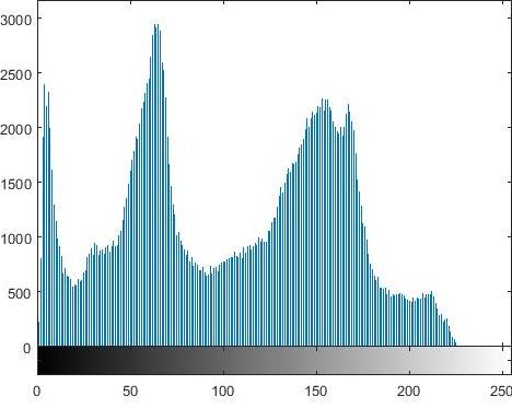
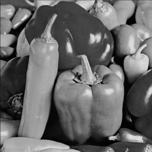
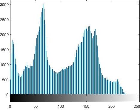
Human observers are the final arbiter of image quality. Therefore, the subjective measure is a perfect way of assessing the quality of the images. Here, we construct stego-images corresponding to different test images used in our experiment for different combinations of $p_{1}$ and $|m|$. This result shows that the stego-images are almost similar to their corresponding cover images. The same is true for their corresponding histograms also. As an example, we present the visual comparison for ‘Pepper’ cover image for one set of parameters; $p_{1}=12$ and $|m|=37$. Fig. 6 shows the (a) ‘Pepper’ cover image (b) ‘Pepper’ cover image histogram (c) ‘Pepper’ stego-image (d) ‘Pepper’ stego-image histogram. From these figures, we observe that the stego-image is almost similar to its corresponding cover image and their corresponding histograms are also very similar.

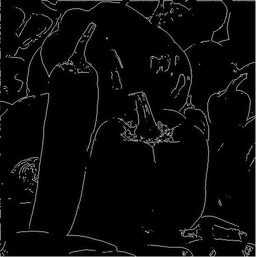
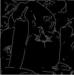
We also construct the edge map diagrams for both the cover image and its corresponding stego-image for this same example. These edge maps are shown in Fig. 7(a) and Fig. 7(b), respectively. We can see from these figures that both the edge maps are almost the same. Hence, the visual quality of the cover image and its corresponding stego-image is almost similar.

(a) ‘Pepper’ cover image

(b) Cover image histogram

(c) ‘Pepper’ stego-image

(d) Stego-image histogram

Figure 6: ‘Pepper’ cover image, its stego-image, and their corresponding histogram using parameter $p_{1}$=12 and $|m|$=37.

(a) Cover image edge map

(b) Stego-image edge map

Figure 7: Edge maps of ‘Pepper’ cover image and its stego-image using parameter $p_{1}$=12 and $|m|$=37.

4.2.2 Objective or Numerical Measures

These measures compare the cover images and their corresponding stego-images based on some numerical criteria that do not require extensive subjective studies. Hence, in recent times, these measures are more commonly used for image quality assessment. These include; Peak Signal-to-Noise Ratio (PSNR), mean Structural Similarity (SSIM) index, Normalized Cross-Correlation (NNC) coefficient, and entropy. We discuss all of them below.

PSNR

We compute the PSNR value to evaluate the imperceptibility of stego-images. That is,

$$PSNR=10\log_{10}\frac{R^{2}}{MSE}\>dB,$$ (20)

where $MSE$ represents the mean square error between the cover image $I$ and the stego-image $SI$, $R$ is the maximum intensity of pixel, which is $255$ for grayscale images, and dB refer to decibel. The $MSE$ is calculated as

$$MSE=\frac{\sum_{i=1}^{r1}\sum_{j=1}^{r2}\left(I\left(i,\,j\right)-SI\left(i,\,j\right)\right)^{2}}{r1\times r2},$$ (21)

where $r1$ and $r2$ represent the row and column numbers of the digital image, respectively, and $I(i,j)$ and $SI(i,j)$ represent the pixel value of the cover image and the constructed stego-image, respectively.

A higher PSNR value indicates the higher imperceptibility of the stego-image. In general, a value higher than 30 dB is considered to be good since human eyes can hardly distinguish the distortion in the stego-image Liu ; Zhang2013 . The PSNR values of the stego-images corresponding to 10 test images of Fig. 4 and 5, and average for all 31 images for different combination of $p_{1}$ and $|m|$ are given in Table 4.2.2. From this table, we can easily observe that this value is higher than 30 dB for all combinations of parameters and for all images.

Value of PSNR (in dB) obtain by proposed CSIS for different parameters and for different test images Test image Parameters $p_{1}=10$ $|m|=32$ $p_{1}=10$ $|m|=35$ $p_{1}=12$ $|m|=37$ $p_{1}=12$ $|m|=40$ $p_{1}=12$ $|m|=42$ $p_{1}=12$ $|m|=47$ $p_{1}=14$ $|m|=36$ $p_{1}=14$ $|m|=39$ Lena 34.34 35.11 35.62 36.15 36.71 37.31 36.33 36.91 Peppers 34.05 34.35 35.23 35.76 36.21 36.98 35.44 35.81 Boat 32.67 33.07 33.84 34.25 34.72 36.84 34.37 34.81 Goldhill 32.69 33.61 34.06 34.54 35.12 35.32 34.33 34.93 Zelda 39.31 39.61 40.10 41.32 40.02 42.67 40.73 42.46 Tiffany 33.64 33.96 34.69 35.88 36.49 37.23 35.73 36.37 Living room 30.94 31.29 32.07 32.98 33.31 33.78 33.48 33.64 Tank 34.27 34.32 35.13 35.62 35.98 36.98 35.36 35.87 Airplane 32.89 34.15 34.88 35.78 36.39 37.91 34.43 35.42 Camera man 35.71 36.89 37.52 38.86 39.38 40.86 40.04 40.65 Avg. of 10 images 34.051 34.636 35.314 36.114 36.433 37.588 36.024 36.687 Avg. of 31 images 34.245 34.883 35.593 36.379 36.668 37.921 36.282 36.901

Means SSIM Index

It is an image quality assessment metric used to measure the structural similarity between two images SSIM . This measure is based on the assumption that the human visual system (HVS) is more adapted to the image's structural information. The mean SSIM (MSSIM) index is given as

$$SSIM(x,y)=\frac{(2\mu_{x}\mu_{y}+C_{1})(2\sigma_{xy}+C_{2})}{(\mu_{x}^{2}+\mu_{y}^{2}+C_{1})(\sigma_{x}^{2}+\sigma_{y}^{2}+C_{2})},$$ (22)

$$MSSIM(I,SI)=\frac{1}{M}\sum_{j=1}^{M}SSIM(i_{j},si_{j}),$$ (23)

where $SSIM(x,y)$ calculates the SSIM index for vectors $x$ and $y$, and $MSSIM$ $(I,SI)$ calculates the mean SSIM between cover image $I$ and stego-image $SI$, i.e. for the overall image quality. Here, $\mu_{x}$ is the weighted mean of $x$, $\mu_{y}$ is the weighted mean of $y$, $\sigma_{x}$ is the weighted standard deviation of $x$, $\sigma_{y}$ is the weighted standard deviation of $y$, $\sigma_{xy}$ is the weighted covariance between $x$ and $y$, $C_{1}$ & $C_{2}$ are arbitrary constants, $i_{j}$ & $si_{j}$ are the content of the cover image and stego-image, respectively, at the $j^{th}$ local window, and $M$ is the number of local windows. We took the values of all these parameters according to SSIM . The value of the mean SSIM index lies between $0$ and $1$, where the value $0$ indicates that there is no similarity between the two images, and the value $1$ indicates that the images are exactly similar.

The mean SSIM index values between the stego-images and their corresponding cover images for different combination of $p_{1}$ and $|m|$ are given in Table 4.2.2. As earlier, 10 images from 4 and 5 are extensively analyze and average of 31 images is reported. From this table, we observe that all these values are close to $1$, which represents that the stego-images are very much similar in structure to their corresponding cover images.

Value of Mean SSIM index obtain by proposed CSIS for different parameters and for different test images Test image Parameter $p_{1}=10$ $|m|=32$ $p_{1}=10$ $|m|=35$ $p_{1}=12$ $|m|=37$ $p_{1}=12$ $|m|=40$ $p_{1}=12$ $|m|=42$ $p_{1}=12$ $|m|=47$ $p_{1}=14$ $|m|=36$ $p_{1}=14$ $|m|=39$ Lena 0.9308 0.9394 0.9475 0.9518 0.9562 0.9672 0.9512 0.9558 Peppers 0.9203 0.9225 0.9291 0.9463 0.9424 0.9547 0.9333 0.9383 Boat 0.9211 0.9356 0.9444 0.9517 0.9575 0.9663 0.9484 0.9545 Goldhill 0.9011 0.9122 0.9236 0.9343 0.9421 0.9532 0.9227 0.9359 Zelda 0.9512 0.9563 0.9613 0.9657 0.9694 0.9768 0.9628 0.9678 Tiffany 0.9239 0.9315 0.9357 0.9434 0.9501 0.9596 0.9369 0.9437 Living room 0.9012 0.9092 0.9211 0.9332 0.9384 0.9460 0.9341 0.9382 Tank 0.8835 0.8857 0.9006 0.9094 0.9197 0.9388 0.9086 0.9131 Airplane 0.9463 0.9525 0.9605 0.9646 0.9673 0.9755 0.9607 0.9692 Camera man 0.9677 0.9752 0.9839 0.9864 0.9871 0.9907 0.9838 0.9868 Avg. of 10 images 0.9198 0.9272 0.9360 0.9445 0.9492 0.9598 0.9398 0.9463 Avg. of 31 Images 0.9206 0.9276 0.9365 0.9449 0.9498 0.9601 0.9412 0.9471

NCC Coefficient

Normalized correlation (NC) metric measures the degree of similarity between two images, and when the two images are independent, this correlation is called normalized cross-correlation (NCC) NC . The NCC coefficient is given as

$$NCC=\frac{\sum_{i=1}^{r1}\sum_{j=1}^{r2}I(i,j)SI(i,j)}{\sum_{i=1}^{r1}\sum_{j=1}^{r2}I^{2}(i,j)},$$ (24)

where $r1$ and $r2$ represent the row and column numbers of the digital image, respectively. $I(i,j)$ and $SI(i,j)$ represent the pixel value of the cover image and the constructed stego-image, respectively. The value equal to 1 indicates that both the images are exactly similar. For our experiments, the values of NCC are given in Table 4.2.2. The set of images used are same as for PSNR and SSIM. We observe that all these values are close to 1, which means that the stego-images are almost identical to their corresponding cover images.

Value of normalized cross-correlation obtain by proposed CSIS for different parameters and for different test images Test image Parameter $p_{1}=10$ $|m|=32$ $p_{1}=10$ $|m|=35$ $p_{1}=12$ $|m|=37$ $p_{1}=12$ $|m|=40$ $p_{1}=12$ $|m|=42$ $p_{1}=12$ $|m|=47$ $p_{1}=14$ $|m|=36$ $p_{1}=14$ $|m|=39$ Lena 0.9985 0.9988 0.9989 0.9991 0.9991 0.9992 0.9991 0.9993 Peppers 0.9982 0.9983 0.9985 0.9987 0.9988 0.9989 0.9985 0.9988 Boat 0.9979 0.9983 0.9985 0.9987 0.9988 0.9989 0.9987 0.9989 Goldhill 0.9976 0.9981 0.9983 0.9986 0.9987 0.9988 0.9982 0.9986 Zelda 0.9991 0.9993 0.9994 0.9995 0.9995 0.9997 0.9994 0.9995 Tiffany 0.9992 0.9993 0.9994 0.9995 0.9995 0.9996 0.9994 0.9995 Living room 0.9962 0.9961 0.9962 0.9971 0.9972 0.9964 0.9970 0.9982 Tank 0.9987 0.9988 0.9992 0.9991 0.9992 0.9993 0.9993 0.9991 Airplane 0.9989 0.9991 0.9993 0.9994 0.9994 0.9995 0.9993 0.9995 Cameraman 0.9989 0.9991 0.9994 0.9994 0.9994 0.9995 0.9995 0.9996 Avg. of 10 images 0.9983 0.9985 0.9989 0.9989 0.9989 0.9989 0.9988 0.9991 Avg. of 31 images 0.9983 0.9985 0.9990 0.9989 0.9989 0.9989 0.9990 0.9991

Entropy

In general, entropy is defined as the measure of average uncertainty of a random variable, which here is the average number of bits required to describe the random variable. In the context of an image, it is a statistical measure of randomness that can be used to characterize the texture of the image Gonzalez . For a grayscale image, entropy is given as

$$Entropy=-\sum_{i=0}^{255}(p_{i}\log_{2}p_{i}),$$ (25)

where $p_{i}$ is the probability of value $i$ pixel of the image. Table 4.2.2 gives the entropy values for the cover images and their corresponding stego-images for different combinations of $p_{1}$ and $|m|$. The set of images used are same as for PSNR, SSIM, and NCC. From this table, we observe that for all these combinations of $p_{1}$ and $|m|$, the entropy of the cover images and their corresponding stego-images are almost similar.

Entropy comparison of cover images and their corresponding stego-images obtain by proposed CSIS using different parameters Test image Cover image Stego-image using different parameters $p_{1}=10$ $|m|=32$ $p_{1}=10$ $|m|=35$ $p_{1}=12$ $|m|=37$ $p_{1}=12$ $|m|=40$ $p_{1}=12$ $|m|=42$ $p_{1}=12$ $|m|=47$ $p_{1}=14$ $|m|=36$ $p_{1}=14$ $|m|=39$ Lena 7.4456 7.4552 7.4581 7..4569 7.456 7.4545 7.4534 7.4551 7.4536 Peppers 7.5715 7.5924 7.5924 7.5908 7.5911 7.5901 7.5889 7.5897 7.5898 Boat 7.1238 7.1323 7.1339 7.1322 7.1334 7.1337 7.1331 7.1277 7.1304 Goldhill 7.4778 7.4653 7.4686 7.4704 7.4723 7.4719 7.4731 7.469 7.4717 Zelda 7.2668 7.2625 7.2635 7.2638 7.2643 7.2649 7.2652 7.2633 7.2642 Tiffany 6.6015 6.6076 6.6063 6.6046 6.606 6.6074 6.607 6.6096 6.6076 Living room 7.2950 7.4200 7.4200 7.4253 7.4260 7.4261 7.4262 7.4267 7.4278 Tank 5.4957 6.3614 6.3728 6.3771 6.3829 6.3846 6.3871 6.3709 6.3815 Airplane 6.7025 6.773 6.7637 6.7535 6.7501 6.7468 6.7396 6.7614 6.7454 Camera man 7.0482 7.0743 7.0763 7.0738 7.0703 7.0683 7.0664 7.0726 7.0661 Avg. of 10 images 7.0028 7.1144 7.0691 7.07678 7.1152 7.1148 7.1140 7.1145 7.1138 Avg. of 31 images 6.9985 6.6451 7.7132 6.7124 6.6476 6.6462 6.6447 6.6469 6.6448

4.3 Security Analysis

Since the proposed CSIS is a transform domain based technique and it employs indirect embedding strategy, i.e. it does not follow the LSB flipping method,and hence, it is immune to statistical attacks Westfeld ; PM1_steganography . Also, CSIS does not lead to the shrinkage effect. That means, after embedding, the nonzero coefficients do not modify to zero value, and hence attacks against F5 Fridrich ; PM1_steganography are not considered.

Moreover, in CSIS, the measurement matrix $\Phi$ is considered as the secret-key, which is shared between the sender and the legitimate receiver. If the eavesdropper intercepts the stego-image by a randomly generated measurement matrix, he cannot not enter the embedding domain without the original secret-key. Hence, we achieve increased security in our proposed system. To justify this, we extract the secret data in two ways, i.e. by using the correct measurement matrix and by using a measurement matrix that is very close to the original one, and obtain the BER (discussed in Section 3.2) between the original secret data the extracted one.

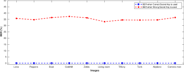
In Fig. 8, we present this BER for earlier discussed 10 cover images, and for the parameter $p_{1}$=12 and $|m|$=37. In this figure, we see that for the correct secret-key, the BER is 0, and for a tiny difference in the measurement matrix, i.e. wrong secret-key, the BER is very high, which is 35% to 40%. That is, even a small change in the secret-key will lead to an extreme shift in accuracy between the original secret data and the extracted one.

Figure 8: BER with the correct and with a wrong secret-key (i.e. measurement matrix)

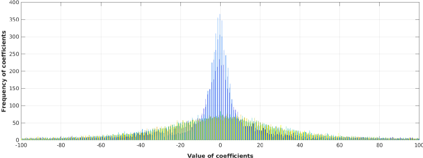
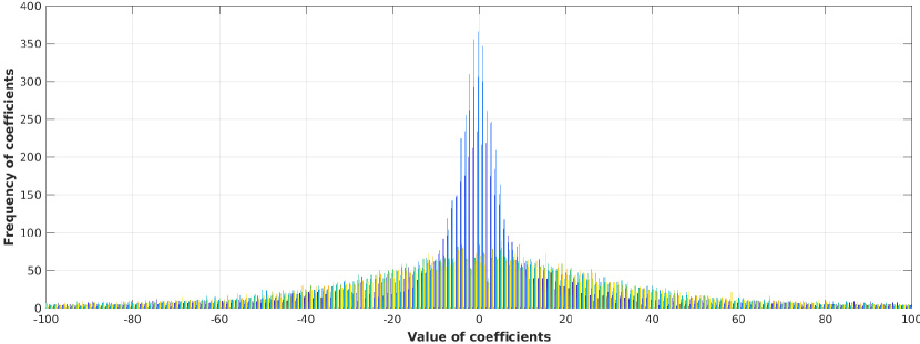
In addition to the above security analysis, we also measure the security by analyzing the distribution of the measurements and their corresponding modified measurements, i.e. after embedding the secret data. For ‘Pepper’ image with parameter $p_{1}$=12 and $|m|$=37, this distribution of the original measurements and the modified measurements is shown in Fig. 9(a) and Fig. 9(b), respectively. The green and blue colors are automatically added by Matlab and do not have any significance here. From these figures, we see that the distribution for both cases is almost the same. We also check these distributions for all the images and obtain the same results. We do not include these in this manuscript due to space limitations.

(a) Original measurements

(b) Modified measurements

Figure 9: Distribution of measurements for ‘Peppers’ image

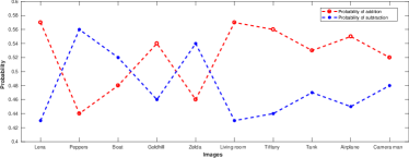
The preservation of distribution of measurements in the earlier two histograms can also be justified by the probability of addition and subtraction operation decided by our algorithm. In Fig. 10, we plot this probability. From this figure, we see that the lines of probabilities of addition and subtraction operation oscillate around 0.5. Here, the minimum and maximum deviation to 0.5 are 0.02 and 0.07, respectively, i.e. for proposed CSIS, the probabilities of both the addition and the subtraction are nearly the same. The distribution of measurements and the probability of addition & subtraction operation as discussed have justified that for our proposed CSIS, the likelihood of detecting data embedding by an eavesdropper is significantly low.

Figure 10: Probability of addition and subtraction operation

4.4 Performance Comparison

In this subsection, we compare the performance of the proposed CSIS with the existing steganography schemes. This result is given in Table 4.4. In this table, the first column represents the comparison metrics, and the remaining columns give the metric data for different steganography schemes.

Performance comparison between proposed CSIS and various other steganography schemes Metrics Steganography Schemes CSIS Ref. Steg_2019_FGT Ref. Jsteg Ref. F5 Ref. Outguess Ref. Liu Ref. Pan Ref. Steg_ExpertSystem Ref. Steg_Rohit Capacity (in bits) 174678 262144 41267 41451 20644 55001 950 57568 113960 PSNR (in dB) 30.94 to 40.86 36.51 34.39 35.00 34.54 32.54 35.52 49.89 36.64 Compression Based Yes No Yes Yes Yes Yes Yes No Yes Resistant to Chi-square Yes No No Yes Yes Yes Yes Yes Yes Resistant to Shrinkage Effect Yes NA Yes No Yes Yes Yes Yes Yes Secret Key Yes No No No No No Yes No No

In the first row of Table 4.4, we compare the average embedding capacity over all the 31 images. We report these embedding capacity for the parameter $p_{1}=12$ & $|m|=37$. In this table, we do not compare these results for all the images because the existing schemes' data are not available for all the images. From the first row of this table, we observe that on an average our steganography scheme has approximately $0.67$, $4.23$, $4.21$, $8.46$, $3.18$, $183.87$, $3.03$ and $1.53$ times embedding capacity as compared to references Steg_2019_FGT , Jsteg , F5 , Outguess , Liu , Pan , Steg_ExpertSystem , and Steg_Rohit , respectively. Here, we can see that our proposed scheme has a higher embedding capacity compared to all schemes except the one, which is Steg_2019_FGT . The reason for this is that this scheme is based on embedding secret data in the spatial domain. As discussed in the Introduction, spatial domain based embedding techniques have a higher embedding capacity, but they are prone to security issues. Also, these techniques are not based on compression, which is the main motivation of this manuscript. Further, as evident from Table 4.1, for a set of parameters $p_{1}=12$ and $|m|=47$, CSIS has 270937, and 251989 bits embedding capacity for the average of 10 and 31 images, respectively. Hence, for this set of parameters, CSIS has approximately the same embedding capacity as that of Steg_2019_FGT .

In the second row of this table, for our scheme we report the range of PSNR values when considering all sets of parameters and again all 31 images. From the second row of this table, we observe that similar to existing steganography schemes, our CSIS also has PSNR values greater than 30 dB, which is considered good Liu ; Zhang2013 .

The purpose of the proposed CSIS is to embed secret data in the compressed domain. Hence, in the third row of Table 4.4, we check which schemes are based on compression and which are not. From this row, we observe that except Steg_2019_FGT ; Steg_ExpertSystem , our CSIS and all other schemes are based on compression. Finally, from the fourth row to the sixth row of Table 4.4, we compare the security of these schemes by checking whether they are resistant to chi-square attack or not, resistant to shrinkage effect or not, and use any secret-key or not. We observe that only our proposed CSIS and Pan schemes pass all the three security tests. Hence, we can conclude that out of all these schemes, only CSIS fulfills all the goals of steganography with higher embedding capacity.

4.5 Experiments on Color Image

All the above experiments were performed on the grayscale images. However, we also show the applicability of our proposed CSIS on a color image. For this we only use ‘Pepper’ color image of resolution $512\times 512$, and perform experiments for $p_{1}=12$ and $|m|=37$ as well as $p_{1}=14$ and $|m|=36$.

The performance analysis of our proposed scheme on color cover image ($512\times 512$ Pepper color image) using different parameters. Parameters Embedding capacity PSNR Mean SSIM Normalized cross-correlation (NCC) (for different color component) Entropy Red Green Blue Average Cover image Stego image $p_{1}=12$, $|m|=37$ 503863 33.89 0.9913 0.9990 0.9981 0.9963 0.9978 7.669 7.723 $p_{1}=14$, $|m|=36$ 573657 33.71 0.9843 0.9989 0.9979 0.9960 0.9976 7.669 7.724 Average 538760 33.80 0.9878 0.9990 0.9980 0.9962 0.9978 7.669 7.723

(a) Color cover image

(b) Color stego image

Figure 11: $512\times 512$ ‘Pepper’ color cover image and stego-image using parameter $p_{1}$=12, $|m|$=37.

Fig. 11 shows the subjective/ visual measure for ‘Pepper’ color image for $p_{1}=12$, $|m|=37$. From this figure, we observe that the cover image and its corresponding stego-image are almost similar. Table 4.5 gives the results for other measures like embedding capacity, PSNR values, mean SSIM index, NCC coefficients for the different color components, and entropy for both cover image and stego-image. We can observe from this table that the embedding capacity of our color image is approximately three times the embedding capacity of ‘Pepper’ grayscale image for the same set of parameters. Please see columns $4$ and $8$ of Table 4.1. This is because of the presence of three color components in the color image. Also, the PSNR values here are greater than 30 dB, and mean SSIM index & NCC coefficients are all close to $1$, which shows that the stego-image is almost similar to its corresponding cover images. Finally, we compare the entropy of the cover image and the stego-image. We see that entropy for both these images is almost the same.

5 Conclusions and Future Work

We present an enhanced-embedding capacity image steganography scheme based on compressed sensing technique. Here, we combine three components to achieve increased embedding capacity without degrading the quality of stego-images, as well as making it resistant to steganalysis attacks. First, we use compressed sensing to sparsify cover image block-wise and obtain its linear measurements using a matrix. We uniquely select a large number of permissible measurements. Hence, we achieve a high embedding capacity. Since the measurement matrix is a secret-key that is shared between the sender and the legitimate receiver, this adds extra security to our scheme. Also, we encrypt the secret data using the DES algorithm and then embed two bits of secret data into each permissible measurement instead of embedding one bit per measurement. Second, we propose a technique of data extraction that is lossless and recovers our secret data entirely. Third, we use ADMM solution of the LASSO formulation of the obtained optimization problem in the stego-image construction. The reason for selecting them is that they have broad applicability in the field of image processing, require less assumptions on the property of the objective function, have fast convergence, and are easy to implement.

We initially perform experiments on several standard grayscale images that vary in texture, and with different sets of parameters and randomly generated binary data as our secret data. For performance evaluation, we calculate embedding capacity, PSNR value, mean SSIM index, NCC coefficient, and entropy. Experiments show that our proposed CSIS achieves higher embedding capacity than existing steganography schemes that follow compression. We achieve 1.53 times more embedding capacity as compared to the most recent scheme of the similar category. PSNR values coming out of our scheme are more than 30 dB, which is considered good. Both mean SSIM index and NCC coefficients values are close to one, which shows that the cover images and their corresponding stego-images are almost similar. This similarity is further supported by the fact that we obtain approximately the same entropy value for both the cover images and their corresponding stego-images. Further, we also show the applicability of CSIS on a color image. Again, the results obtained are almost the same as that of grayscale images. However, we get approximately three times higher embedding capacity for the color image because of the presence of the three component in color images.

In future, we plan to embed the secret data in text, audio, and video. Other future works include extending this work for a real-time application such as hiding fingerprint data, iris data, medical information of patients, and personal signature. As mentioned in the Introduction, another line of work is embedding images inside images. Since a lot of work has been done in embedding a single image, we will focus on hiding multiple secret images and multilevel image steganography scheme.

References

- [1] W. Stallings, Cryptography and network security: principles and practice. Prentice Hall, 2019.
- [2] M. Khodaei and K. Faez, “New adaptive steganographic method using least-significant-bit substitution and pixel-value differencing,” IET Image processing, vol. 6, no. 6, pp. 677–686, 2012.
- [3] N. Alanazi, E. Khan, and A. Gutub, “Efficient security and capacity techniques for arabic text steganography via engaging unicode standard encoding,” Multimedia Tools and Applications, Accessed on 22 October 2019. [Online] https://link.springer.com/article/10.1007/s11042-020-09667-y.
- [4] L. Xiang, S. Yang, Y. Liu, Q. Li, and C. Zhu, “Novel linguistic steganography based on character-level text generation,” Mathematics, vol. 8, no. 9, p. 1558, 2020.
- [5] S. Sarreshtedari and M. A. Akhaee, “One-third probability embedding: a new 1 histogram compensating image least significant bit steganography scheme,” IET image processing, vol. 8, no. 2, pp. 78–89, 2013.
- [6] S. Devi, M. N. Sahoo, K. Muhammad, W. Ding, and S. Bakshi, “Hiding medical information in brain MR images without affecting accuracy of classifying pathological brain,” Future Generation Computer Systems, vol. 99, pp. 235 – 246, 2019.
- [7] S. Khan, T. Khan, T. Mahmood, and N. Ahmad, “Analysis of data hiding in R, G and B channels of color image using various number of LSBs,” in 2016 Sixth International Conference on Innovative Computing Technology (INTECH), pp. 270–274, IEEE, 2016.
- [8] A. Ul Islam, F. Khalid, M. Shah, Z. Khan, T. Mahmood, A. Khan, U. Ali, and M. Naeem, “An improved image steganography technique based on MSB using bit differencing,” in 2016 Sixth International Conference on Innovative Computing Technology (INTECH), pp. 265–269, IEEE, 2016.
- [9] W. Zhang, Z. Zhang, L. Zhang, H. Li, and N. Yu, “Decomposing joint distortion for adaptive steganography,” IEEE Transactions on Circuits and Systems for Video Technology, vol. 27, no. 10, pp. 2274–2280, 2017.
- [10] A. Rehman, T. Saba, T. Mahmood, Z. Mehmood, M. Shah, and A. Anjum, “Data hiding technique in steganography for information security using number theory,” Journal of Information Science, vol. 45, no. 6, pp. 767–778, 2018.
- [11] M. Shah, W. Zhang, H. Hu, H. Zhou, and T. Mahmood, “Homomorphic encryption-based reversible data hiding for 3D mesh models,” Arabian Journal for Science and Engineering, vol. 43, pp. 8145–8157, 2018.
- [12] JSteg Source, Last accessed on 22 October 2019. https://zooid.org/~paul/crypto/jsteg/.
- [13] A. Westfeld, “F5—a steganographic algorithm,” in Information Hiding (I. S. Moskowitz, ed.), vol. 2137, pp. 289–302, Springer Berlin Heidelberg, 2001.
- [14] N. Provos, “Defending against statistical steganalysis,” in Proceedings of the 10th Conference on USENIX Security Symposium, vol. 10 of SSYM’01, pp. 323–336, USENIX Association, 2001.
- [15] C.-C. Chang, T.-S. Chen, and L.-Z. Chung, “A steganographic method based upon JPEG and quantization table modification,” Information Sciences, vol. 141, no. 1, pp. 123–138, 2002.
- [16] C.-L. Liu and S.-R. Liao, “High-performance JPEG steganography using complementary embedding strategy,” Pattern Recognition, vol. 41, no. 9, pp. 2945–2955, 2008.
- [17] J.-S. Pan, W. Li, C.-S. Yang, and L.-J. Yan, “Image steganography based on subsampling and compressive sensing,” Multimedia Tools and Applications, vol. 74, no. 21, pp. 9191–9205, 2015.
- [18] H. Al-Dmour and A. Al-Ani, “A steganography embedding method based on edge identification and XOR coding,” Expert Systems with Applications, vol. 46, pp. 293–306, 2016.
- [19] A. K. Pal, K. Naik, and R. Agrawal, “A steganography scheme on JPEG compressed cover image with high embedding capacity,” The International Arab Journal of Information Technology, vol. 16, no. 1, pp. 116–124, 2019.
- [20] D. R. I. M. Setiadi and E. H. Rachmawanto, “Secure image steganography algorithm based on DCT with OTP encryption,” Journal of Applied Intelligent System, vol. 2, no. 1, pp. 1–11, 2017.
- [21] Y. Zhang, C. Qin, W. Zhang, F. Liu, and X. Luo, “On the fault-tolerant performance for a class of robust image steganography,” Signal Processing, vol. 146, pp. 99–111, 2018.
- [22] J. Tao, S. Li, X. Zhang, and Z. Wang, “Towards robust image steganography,” IEEE Transactions on Circuits and Systems for Video Technology, vol. 29, no. 2, pp. 594–600, 2019.
- [23] R. Agrawal, “SABMIS: -minimization and sparse approximation based blind multi-image steganography scheme,” Tech. Rep. arXiv:2007.05025 [cs.MM], ArXiV, 2020. https://arxiv.org/abs/2007.05025 .
- [24] A. Westfeld and A. Pfitzmann, “Attacks on steganographic systems,” in Information Hiding (A. Pfitzmann, ed.), vol. 1768, pp. 61–76, Springer Berlin Heidelberg, 2000.
- [25] J. Fridrich, M. Goljan, and D. Hogea, “Steganalysis of JPEG images: Breaking the F5 algorithm,” in Information Hiding (F. A. P. Petitcolas, ed.), vol. 2578, pp. 310–323, Springer Berlin Heidelberg, 2003.
- [26] C. Patsakis, N. Aroukatos, and S. Zimeras, “LSB steganographic detection using compressive sensing,” in Intelligent Interactive Multimedia Systems and Services (G. A. Tsihrintzis, M. Virvou, L. C. Jain, and R. J. Howlett, eds.), vol. 11, pp. 219–225, Springer Berlin Heidelberg, 2011.
- [27] S. Arunkumar, V. Subramaniyaswamy, V. Vijayakumar, N. Chilamkurti, and R. Logesh, “SVD-based robust image steganographic scheme using RIWT and DCT for secure transmission of medical images,” Measurement, vol. 139, pp. 426–437, 2019.
- [28] A. V. Sreedhanya and K. P. Soman, “Ensuring security to the compressed sensing data using a steganographic approach,” Bonfring International Journal of Advances in Image Processing, vol. 3, no. 1, pp. 01–07, 2013.
- [29] R. Thanki, S. Borra, V. Dwivedi, and K. Borisagar, “A steganographic approach for secure communication of medical images based on the DCT-SVD and the compressed sensing (CS) theory,” The Imaging Science Journal, vol. 65, no. 8, pp. 457–467, 2017.
- [30] C. Patsakis and N. Aroukatos, “A DCT steganographic classifier based on compressive sensing,” in 2011 Seventh International Conference on Intelligent Information Hiding and Multimedia Signal Processing, pp. 169–172, IEEE, 2011.
- [31] H. Zhao, J. Ren, J. Zhan, Y. Xiao, S. Y. Zhao, F. Lei, M. Assaad, and C. Li, “Compressive sensing based secret signals recovery for effective image steganalysis in secure communications,” Multimedia Tools and Applications, vol. 78, pp. 29381–29394, 2019.
- [32] E. J. Candès, J. Romberg, and T. Tao, “Robust uncertainty principles: exact signal reconstruction from highly incomplete frequency information,” IEEE Transactions on Information Theory, vol. 52, no. 2, pp. 489–509, 2006.
- [33] D. L. Donoho, “Compressed sensing,” IEEE Transactions on Information Theory, vol. 52, no. 4, pp. 1289–1306, 2006.
- [34] J. Romberg, “Imaging via compressive sampling,” IEEE Signal Processing Magazine, vol. 25, no. 2, pp. 14–20, 2008.
- [35] R. Baraniuk and P. Steeghs, “Compressive radar imaging,” in 2007 IEEE Radar Conference, pp. 128–133, IEEE, 2007.
- [36] J. Chul Ye, “Compressed sensing MRI: a review from signal processing perspective,” BMC Biomedical Engineering, vol. 1, no. 8, pp. 1–17, 2018.
- [37] E. J. Candès, “The restricted isometry property and its implications for compressed sensing,” Comptes Rendus Mathematique, vol. 346, no. 9, pp. 589–592, 2008.
- [38] L. Ji-xin, L. Xiao-fei, H. Guang, S. Ning, D. Kun, and S. Quan-sen, “Colour compressed sensing imaging via sparse difference and fractal minimisation recovery,” IET Image Processing, vol. 9, no. 5, pp. 369–380, 2014.
- [39] H. Yuan, H. Song, X. Sun, K. Guo, and Z. Ju, “Compressive sensing measurement matrix construction based on improved size compatible array LDPC code,” IET Image Processing, vol. 9, no. 11, pp. 993–1001, 2015.
- [40] T. T. Cai and L. Wang, “Orthogonal matching pursuit for sparse signal recovery with noise,” IEEE Transactions on Information theory, vol. 57, no. 7, pp. 4680–4688, 2011.
- [41] D. Needell and J. A. Tropp, “CoSaMP: Iterative signal recovery from incomplete and inaccurate samples,” Applied and Computational Harmonic Analysis, vol. 26, no. 3, pp. 301–321, 2009.
- [42] S. J. Wright, R. D. Nowak, and M. A. T. Figueiredo, “Sparse reconstruction by separable approximation,” IEEE Transactions on Signal Processing, vol. 57, no. 7, pp. 2479–2493, 2009.
- [43] W. Chen, D. Wipf, Y. Wang, Y. Liu, and I. J. Wassell, “Simultaneous Bayesian sparse approximation with structured sparse models,” IEEE Transactions on Signal Processing, vol. 64, no. 23, pp. 6145–6159, 2016.
- [44] S. Boyd, N. Parikh, E. Chu, B. Peleato, and J. Eckstein, “Distributed optimization and statistical learning via the alternating direction method of multipliers,” Foundations and Trends in Machine Learning, vol. 3, no. 1, pp. 1–122, 2011.
- [45] H. J. Hwang, S. Kim, and H. J. Kim, “Reversible data hiding using least square predictor via the LASSO,” EURASIP Journal on Image and Video Processing, vol. 2016, no. 1, p. 42, 2016.
- [46] R. Agrawal, K. Ahuja, C. H. Hoo, T. D. A. Nguyen, and A. Kumar, “ParaLarPD: Parallel FPGA router using primal-dual sub-gradient method,” Electronics, vol. 8, no. 12, p. 1439, 2019.
- [47] M. S. Asif and J. Romberg, “Dynamic updating for minimization,” IEEE Journal of selected topics in signal processing, vol. 4, no. 2, pp. 421–434, 2010.
- [48] E. Candès and J. Romberg, “Sparsity and incoherence in compressive sampling,” Inverse problems, vol. 23, no. 3, pp. 969–985, 2007.
- [49] X. Xu, J. Zhang, A. Huang, and B. Jiang, “An adaptive measurement scheme based on compressed sensing for wideband spectrum detection in cognitive WSN,” Journal of Electronics (China), vol. 29, no. 6, pp. 585–592, 2012.
- [50] U. Dias and M. E. Rane, “Comparative analysis of sensing matrices for compressed sensed thermal images,” in 2013 International Mutli-Conference on Automation, Computing, Communication, Control and Compressed Sensing (iMac4s), pp. 265–270, IEEE, 2013.
- [51] The USC-SIPI Images Database, Last accessed on 22 October 2019. http://sipi.usc.edu/database/.
- [52] Images Database, Last accessed on 22 October 2019. https://homepages.cae.wisc.edu/~ece533/images/.
- [53] Images Database, Last accessed on 22 October 2019. http://imageprocessingplace.com/root_files_V3/image_databases.htm.
- [54] S. A. Parah, J. A. Sheikh, N. A. Loan, and G. M. Bhat, “Robust and blind watermarking technique in DCT domain using inter-block coefficient differencing,” Digital Signal Processing, vol. 53, pp. 11–24, 2016.
- [55] Y. Zhang, J. Jiang, Y. Zha, H. Zhang, and S. Zhao, “Research on embedding capacity and efficiency of information hiding based on digital images,” International Journal of Intelligence Science, vol. 3, no. 02, pp. 77–85, 2013.
- [56] W. Habib, T. Sarwar, A. M. Siddiqui, and I. Touqir, “Wavelet denoising of multiframe optical coherence tomography data using similarity measures,” IET Image Processing, vol. 11, no. 1, pp. 64–79, 2016.
- [57] R. C. Gonzalez, R. E. Woods, and S. L. Eddins, Digital image processing using MATLAB. Pearson Education India, 2004.
- [58] L. Yu, Y. Zhao, R. Ni, and Z. Zhu, “PM1 steganography in JPEG images using genetic algorithm,” Soft Computing, vol. 13, no. 4, pp. 393–400, 2009.