$k$-Inflation-corrected Einstein-Gauss-Bonnet Gravity with Massless Primordial Gravitons

Abstract

In the present paper, we study the inflationary phenomenology of a $k$-inflation corrected Einstein-Gauss-Bonnet theory. Non-canonical kinetic terms are known for producing Jean instabilities or superluminal sound wave velocities in the aforementioned era, but we demonstrate in this work that by adding Gauss-Bonnet string corrections and assuming that the non-canonical kinetic term $\omega X^{\gamma}$ is in quadratic, one can obtain a ghost free description. Demanding compatibility with the recent GW170817 event forces one to accept that the relation $\ddot{\xi}=H\dot{\xi}$ for the scalar coupling function $\xi(\phi)$. As a result, the scalar functions of the theory are revealed to be interconnected and by assuming a specific form for one of them, specifies immediately the other. Here, we shall assume that the scalar potential is directly derivable from the equations of motion, once the Gauss-Bonnet coupling is appropriately chosen, but obviously the opposite is feasible as well. As a result, each term entering the equations of motion, can be written in terms of the scalar field and a relatively tractable phenomenology is produced. For quadratic kinetic terms, the resulting scalar potential is quite elegant functionally. Different exponents, which lead to either a more perplexed solution for the scalar potential, are still a possibility which was not further studied. We also discuss in brief the non-Gaussianities issue under the slow-roll and constant-roll conditions holding true, and we demonstrate that the predicted amount of non-Gaussianities is significantly enhanced in comparison to the $k$-inflation free Einstein-Gauss-Bonnet theory.

I Introduction

Describing the inflationary era in a consistent way is one of the main task in modern theoretical cosmology. To date, there are two main ways to describe the inflationary era, with the first being by using the single scalar field description Guth:1980zm ; Linde:1993cn ; Linde:1983gd , while the other is by using the modified gravity description Nojiri:2017ncd ; Nojiri:2010wj ; Nojiri:2006ri ; Capozziello:2011et ; Capozziello:2010zz ; Olmo:2011uz . Both ways are appealing, however the modified gravity description is somewhat more complete since it offers the appealing possibility of describing the inflationary and the dark energy era by using the same theoretical framework Nojiri:2003ft ; Odintsov:2020iui ; Odintsov:2020nwm ; Sa:2020qfd . Of course we need also to mention that bouncing cosmology is an also quite appealing alternative to inflation bounces . On the other hand, string theory is to date the most complete high energy completion of general relativity and of the Standard Model, and it is therefore natural to assume that it will have some imprints on the low-energy inflationary Lagrangian. It is a well known fact that the inflationary era is essentially a classical theory, in which era, the Universe is four dimensional and also evolves in a classical way, with quantum effects affecting the evolution in a subdominant way. In this sense, Einstein-Gauss-Bonnet theories Hwang:2005hb ; Nojiri:2006je ; Cognola:2006sp ; Nojiri:2005vv ; Nojiri:2005jg ; Satoh:2007gn ; Bamba:2014zoa ; Yi:2018gse ; Guo:2009uk ; Guo:2010jr ; Jiang:2013gza ; Kanti:2015pda ; vandeBruck:2017voa ; Kanti:1998jd ; Pozdeeva:2020apf ; Fomin:2020hfh ; DeLaurentis:2015fea ; Chervon:2019sey ; Nozari:2017rta ; Odintsov:2018zhw ; Kawai:1998ab ; Yi:2018dhl ; vandeBruck:2016xvt ; Kleihaus:2019rbg ; Bakopoulos:2019tvc ; Maeda:2011zn ; Bakopoulos:2020dfg ; Ai:2020peo ; Odintsov:2019clh ; Oikonomou:2020oil ; Odintsov:2020xji ; Oikonomou:2020sij ; Odintsov:2020zkl ; Odintsov:2020sqy ; Odintsov:2020mkz ; Easther:1996yd ; Antoniadis:1993jc ; Antoniadis:1990uu ; Kanti:1995vq ; Kanti:1997br . have an elevated role in the description of the inflationary era, since these theories provide a string-motivated modification of the canonical scalar field inflationary theory, with the low-energy string corrections appearing as Gauss-Bonnet corrections. However, the GW170817 event back in 2017 GBM:2017lvd altered the perception of the viability of a modified gravity theory, since, the gravitational wave speed was found to have the same propagation speed as that of lights. Since there is no fundamental reason coming from particle physics which indicates that the graviton should change its mass, at least to our knowledge, it is natural to assume that the primordial gravitational waves should have a propagation speed equal to unity in natural units. This sole constraint has already excluded many theories that predicted a primordial tensor mode spectrum with propagation speed different that that of light’s, see for example Ezquiaga:2017ekz , and Einstein-Gauss-Bonnet theories belong to this class of excluded theories. In some recent works we introduced a new formalism that offers a remedy to the non-viability issue of Einstein-Gauss-Bonnet theories and related theories, in view of the GW170817 event Odintsov:2019clh ; Oikonomou:2020oil ; Odintsov:2020xji ; Odintsov:2020zkl ; Odintsov:2020sqy ; Oikonomou:2020sij ; Odintsov:2020mkz . The basic new feature of these new theories which are GW170817 compatible, is that the scalar potential and the Gauss-Bonnet scalar coupling function should no longer be considered as independent functions that can be freely chosen, but these must be related in a specific way.

In this work, we extend the theoretical framework of GW170817-compatible Einstein-Gauss-Bonnet theories, to include $k$-inflation corrections ArmendarizPicon:1999rj ; Chiba:1999ka ; ArmendarizPicon:2000dh ; Matsumoto:2010uv ; ArmendarizPicon:2000ah ; Chiba:2002mw ; Malquarti:2003nn ; Malquarti:2003hn ; Chimento:2003zf ; Chimento:2003ta ; Scherrer:2004au ; Aguirregabiria:2004te ; ArmendarizPicon:2005nz ; Abramo:2005be ; Rendall:2005fv ; Bruneton:2006gf ; dePutter:2007ny ; Babichev:2007dw ; Deffayet:2011gz ; Kan:2018odq ; Unnikrishnan:2012zu ; Li:2012vta , thus non-canonical higher order kinetic terms for the scalar field. The motivation for this addition is three fold: Firstly in order to see whether a viable inflationary phenomenology can be generated in this case, secondly in order to see whether the non-Gaussianities are enhanced in this case, and thirdly, $k$-inflation might offer the possibility of also describing the dark energy era. The focus in this paper will be on the first two aforementioned issues, namely the inflationary phenomenology and the non-Gaussianities issue, and as we demonstrate, it is possible to produce viable inflationary phenomenology, and also the non-Gaussianities of the primordial power spectrum are significantly enhanced in comparison to the $k$-inflation free Einstein-Gauss-Bonnet theory.

II Einstein-Gauss-Bonnet $k$-Inflation Dynamics

We commence by defining the gravitational action corresponding to an $k$-Inflation-corrected Einstein-Gauss-Bonnet gravity, which is,

$$\centering S=\int{d^{4}x\sqrt{-g}\left(\frac{R}{2\kappa^{2}}-\alpha X-\omega X^{\gamma}-V(\phi)-\xi(\phi)\mathcal{G}\right)},\,\@add@centering$$ (1)

with $R$ being the Ricci scalar, $\kappa=\frac{1}{M_{P}}$ the gravitational constant and $M_{P}$ the reduced Planck mass, while $X=\frac{1}{2}g^{\mu\nu}\partial_{\mu}\phi\partial_{\nu}\phi$ and $V(\phi)$ are the kinetic term and scalar potential. Also $\mathcal{G}$ denotes the Gauss-Bonnet invariant defined as $\mathcal{G}=R^{2}-4R_{\mu\nu}R^{\mu\nu}+R_{\mu\nu\sigma\rho}R^{\mu\nu\sigma\rho}$ with $R_{\mu\nu}$ and $R_{\mu\nu\sigma\rho}$ being the Ricci and Riemann tensor respectively and lastly, $\xi(\phi)$ signifies the Gauss-Bonnet scalar coupling function. Concerning the non-canonical kinetic term, we mention that $\omega$ is a constant with mass dimensions [m]^4-4γ for consistency. Similarly, $\alpha$ shall take the values $0,1$ but we shall leave it as it is in order to have the phantom case available for the reader. In the present paper, we shall also assume that the cosmological background corresponds to that of a flat Friedman-Robertson-Walker (FRW) metric, with the line element being,

$$\centering ds^{2}=-dt^{2}+a^{2}(t)\delta_{ij}dx^{i}dx^{j},\,\@add@centering$$ (2)

where $a(t)$ denotes the scale factor. In consequence, the Ricci and Gauss-Bonnet scalars are written as $R=12H^{2}+6\dot{H}$ and $\mathcal{G}=24H^{2}(\dot{H}+H^{2})$, with $H$ being Hubble’s parameter $H=\frac{\dot{a}}{a}$ and the “dot” signifies differentiation with respect to the cosmic time. Furthermore, by assuming that the scalar field is homogeneous, then the kinetic term is simplified greatly as now $X=-\frac{1}{2}\dot{\phi}^{2}$. Due to this definition, we shall limit our work to only integer values for $\gamma$ in order to avoid the emergence of complex numbers.

Theories with non-canonical kinetic terms are known for producing a formula for the velocity of the gravitational waves with does not necessarily coincide with the speed of light. Before we proceed with the equations of motion, it is worth taking care of the constraints imposed by the GW170817 event. In order for this particular model not to be at variance with the GW170817 event, we demand that in natural units where $c=1$, the velocity of the gravitational waves is equal to unity. Thus,

$$\centering c_{T}^{2}=1-\frac{Q_{f}}{2Q_{t}},\,\@add@centering$$ (3)

must be equated to unity. Here, we make use of certain auxiliary functions defined as $Q_{f}=16(\ddot{\xi}-H\dot{\xi})$ and $Q_{t}=\frac{1}{\kappa^{2}}-8\dot{\xi}H$. As a result, compatibility is restored once the numerator of the second term is equated to zero, meaning that $\ddot{\xi}=H\dot{\xi}$. This case was studied in Odintsov:2020sqy for the slow-roll case and in turn, the following differential equation was found to constraint the functional form of the Gauss-Bonnet coupling,

$$\centering\dot{\phi}\simeq H\frac{\xi^{\prime}}{\xi^{\prime\prime}}\,.\@add@centering$$ (4)

where “prime” denotes differentiation with respect to the scalar field $\phi$.

The gravitational action is a powerful tool since it contains stored all the available information about the inflationary era. Implementing the variation principle with respect to the metric tensor and the scalar potential, produces the gravitational field equation and also the continuity equation of the scalar field. By separating the equations of motion in time and space components, the equations of motion are derived which read,

$$\centering\frac{3H^{2}}{\kappa^{2}}=-\alpha X+\omega(1-2\gamma)X^{\gamma}+V(\phi)+24\dot{\xi}H^{3},\,\@add@centering$$ (5)

$$\centering\dot{H}=\kappa^{2}(\alpha X+\omega\gamma X^{\gamma}+8\dot{\xi}H\dot{H}),\,\@add@centering$$ (6)

$$\centering\alpha(\ddot{\phi}+3H\dot{\phi})+(\ddot{\phi}(2\gamma-1)+3H\dot{\phi})\omega\gamma X^{\gamma-1}+V^{\prime}+\xi^{\prime}\mathcal{G}=0,\,\@add@centering$$ (7)

where for $\gamma\to 1$ one obtains the usual Einstein-Gauss-Bonnet equations of motion. This is the set of differential equations that must be solved in order to extract results for a given model during the inflationary era. However, this model is hard to solve analytically, hence, certain approximations must be made in order to proceed. Here, we shall make two kinds of approximations. The first is the slow-roll approximation, where one assumes that the scalar field has an inferior canonical kinetic term compared to the scalar potential. This approximation will be extended to the non-canonical kinetic term as well, hence the slow-roll approximations are,

$$\centering\dot{H}\@add@centering \ll H^{2}, \alpha X+\omega X^{\gamma} \ll V \ddot{\phi} \ll H\dot{\phi}.\,$$ (8)

These inequalities refer to the order of magnitude and not the sign of each term. Subsequently, the equations of motion can be simplified greatly,

$$\centering H^{2}\simeq\frac{\kappa^{2}V}{3},\,\@add@centering$$ (9)

$$\centering\dot{H}\simeq\kappa^{2}(\alpha X+\omega\gamma X^{\gamma}).\,\@add@centering$$ (10)

$$\centering V^{\prime}+3H\dot{\phi}(\alpha+\omega\gamma X^{\gamma-1})\simeq 0,\,\@add@centering$$ (11)

Let us now proceed with the designation of certain auxiliary parameters which shall play a significant role in subsequent calculations. These parameters are slowly varying obviously. Firstly, we define the set of the slow-roll indices as,

$$\centering\epsilon_{1}\@add@centering =-\frac{\dot{H}}{H^{2}}, \epsilon_{2} =\frac{\ddot{\phi}}{H\dot{\phi}}, \epsilon_{3} =0, \epsilon_{5} =\frac{Q_{a}}{2HQ_{t}}, \epsilon_{6} =\frac{\dot{Q}_{t}}{2HQ_{t}},\,$$ (12)

where $Q_{a}=-8\dot{\xi}H^{2}$ and again, $Q_{t}=\frac{1}{\kappa^{2}}-8\dot{\xi}H$. Here, the index $\epsilon_{4}$ was omitted simply because it is of no interest. The same can be said about indices $\epsilon_{5}$ and $\epsilon_{6}$ but since they are derived from the string corrections, they are presented for the sake of completeness. Moreover, the functions which shall be utilized have the following form,

$$\centering\delta_{\xi}\@add@centering =\kappa^{2}H\dot{\xi}, \epsilon_{s} =\epsilon_{1}-4\delta_{\xi}, \eta_{s} =\frac{\dot{\epsilon}_{s}}{H\epsilon_{s}}, s =\frac{\dot{c}_{s}}{Hc_{s}}.$$ (13)

These functions are of paramount importance since they are strongly connected with the observed quantities as we shall show in the following. Before we proceed with the observational quantities however, we note that $c_{s}$ is the field propagation velocity defined as,

$$\centering c_{s}^{2}=\kappa^{4}\frac{2\omega_{1}^{2}\omega_{2}H-\omega_{2}^{2}\omega_{1}+4\omega_{1}\dot{\omega}_{1}\omega_{2}-2\omega_{1}^{2}\dot{\omega}_{2}}{4\Sigma}\@add@centering$$ (14)

where,

$$\centering\Sigma=\kappa^{4}\frac{\omega_{1}(4\omega_{1}\omega_{3}+9\omega_{2}^{2})}{12},\,\@add@centering$$ (15)

$$\centering\omega_{1}=Q_{t},\,\@add@centering$$ (16)

$$\centering\omega_{2}=\frac{2H}{\kappa^{2}}-24H^{2}\dot{\xi},\,\@add@centering$$ (17)

$$\centering\omega_{3}=-\left(\frac{3H}{\kappa}\right)^{2}-3\alpha X-3\omega\gamma(2\gamma-1)X^{\gamma}+144H^{3}\dot{\xi},\,\@add@centering$$ (18)

Finally, the predicted amount of non-Gaussianities for each model can be evaluated from the equilateral non-linear term DeFelice:2011zh ,

$$\centering f_{NL}^{eq}=\frac{85}{324}\left(1-\frac{1}{c_{s}^{2}}\right)-\frac{10}{81}\frac{\lambda}{\Sigma}+\frac{55}{36}\frac{\epsilon_{s}}{c_{s}^{2}}+\frac{5}{12}\frac{\eta_{s}}{c_{s}^{2}}-\frac{85}{54}\frac{s}{c_{s}^{2}}-\frac{10}{81}\delta_{\xi}\left(2-\frac{29}{c_{s}^{2}}\right),\,\@add@centering$$ (19)

with $\lambda$ being,

$$\centering\lambda=-\omega\gamma(\gamma-1)X^{\gamma}\left(1+\frac{2(\gamma-2)}{3}\right).\,\@add@centering$$ (20)

In the case of Einstein-Gauss-Bonnet gravity with canonical kinetic term, the expected deviation from the Gaussian distribution is small while on the other hand, the non-Gaussianities are now expected to be enhanced due to the inclusion of a non-canonical kinetic term. Finally, the observed quantities which shall be evaluated and compared to the recent Planck 2018 data are the scalar spectral index of primordial curvature perturbations $n_{S}$, the spectral index of tensor perturbations $n_{T}$ and the tensor-to-scalar ratio $r$, connected to the previously defined slow-roll parameters as shown below,

$$\centering n_{S}\@add@centering =1-2\epsilon_{1}-\eta_{s}-s, n_{T} =-2\epsilon_{1}, r =16\epsilon_{s}c_{s},\,$$ (21)

with the corresponding values being

$$\centering n_{S}\@add@centering =0.9649\pm 0.0042,68\%C.L r <0.064,95\%C.L,\,$$ (22)

The main goal is to evaluate those quantities during the first horizon crossing by finding the initial value of the scalar field. One can evaluate the final value of the scalar field in the first place by simply assuming that the slow-roll index $\epsilon_{1}$ becomes of order $\mathcal{O}(1)$. The initial value in turn can be evaluated from the $e$-foldings number, since in this framework, it is equal to,

$$\centering N=\int_{\phi_{i}}^{\phi_{f}}{\frac{\xi^{\prime\prime}}{\xi^{\prime}}d\phi}\,,\@add@centering$$ (23)

Although the procedure seems tedious, one must be wary not to produce Jeans instabilities, meaning field propagation velocities which obey the relation $c_{s}^{2}<0$ and also superluminal velocities where $c_{s}>1$. The latter case does not respect causality, but there exist certain cases which produce such result, therefore they should be avoided. In the following, we shall study simple coupling functions which manage to simplify the ratio $\xi^{\prime}/\xi^{\prime\prime}$ which appears in the equations of motion. These functions were proved to be capable of producing a viable phenomenology in the canonical case.

III Confronting String Corrected k-Inflation with Observations

In this section, we present a variety of models which have been studied in previous works of ours Odintsov:2019clh ; Oikonomou:2020oil ; Odintsov:2020xji ; Odintsov:2020zkl ; Odintsov:2020sqy ; Oikonomou:2020sij ; Odintsov:2020mkz , using the canonical kinetic term in Einstein-Gauss-Bonnet gravity theory. We shall also show that apart from being viable, the models are also capable of predicting a larger amount of non-Gaussianities which is an important distinction between the $k$-inflation and the ordinary Einstein-Gauss-Bonnet models.

III.1 Error Function Model in the Presence of a Higher Order Kinetic Term

Let us assume that the coupling function is that of Eq. (39) with $\alpha=1$ and $\gamma=2$. Also, in order to avoid confusion between the models, we shall use subscripts in similar parameters. The subscript in the first model is 1. Hence, let the Gauss-Bonnet coupling be,

$$\centering\xi(\phi)=\frac{2\Lambda_{1}}{\sqrt{\pi}}\int_{0}^{\delta_{1}\kappa\phi}{e^{-x^{2}}dx}\,,\@add@centering$$ (24)

As a result, Eq. (11) produces the following scalar potential,

$$\centering V(\phi)=\frac{12\delta_{1}^{4}(\alpha-4\delta_{1}^{2})}{\omega}(\kappa\phi)^{2}\,,\@add@centering$$ (25)

where the integration constant is set equal to zero for simplicity. In turns out that the scalar potential has an elegant power-law form and specifically it follows a squared law form. Then consequently,

$$\centering\epsilon_{1}=\frac{1}{2(\delta_{3}\kappa\phi)^{2}}\,,\@add@centering$$ (26)

$$\centering\epsilon_{2}=0\,,\@add@centering$$ (27)

$$\centering\epsilon_{5}=\frac{4\Lambda_{1}\kappa^{4}V(\phi)}{3\sqrt{\pi}\delta_{1}\kappa\phi e^{(\delta_{1}\kappa\phi)^{2}}+8\Lambda_{1}\kappa^{4}V(\phi)}\,,\@add@centering$$ (28)

$$\centering\epsilon_{6}=\frac{2\Lambda_{1}\left(\kappa^{4}V(\phi)(2(\delta_{1}\kappa\phi)^{2}+1)-\kappa\phi\kappa^{3}V^{\prime}(\phi)\right)}{(\delta_{1}\kappa\phi)^{2}\left(3\sqrt{\pi}\delta_{1}\kappa\phi e^{(\delta_{1}\kappa\phi)^{2}}+8\Lambda_{1}\kappa^{4}V(\phi)\right)}\,,\@add@centering$$ (29)

$$\centering\delta_{\xi}=-\frac{\kappa^{3}\xi^{\prime}(\phi)V(\phi)}{6\delta_{1}^{2}\kappa\phi}\,,\@add@centering$$ (30)

$$\centering\lambda=-\frac{\omega}{2}\left(\frac{V(\phi)}{12(\delta_{3}^{2}\kappa\phi)^{2}}\right)^{2}\,,\@add@centering$$ (31)

These are the the only simple auxiliary parameters of the model and each quantity can be constructed from them. It is worth mentioning that $\epsilon_{2}=0$ or in other words $\ddot{\phi}=0$. Thus, $\phi(t)$ is a simple linear function of time and hence the time duration of the inflationary era can be extracted for the initial and final value of the scalar field. These values can be evaluated from the condition $\epsilon_{1}(\phi_{f})=1$, which terminates inflation and afterwards the value $\phi_{i}$ if the scalar field, during the first horizon crossing, can be derived from the $e$-folding number (23). As a result, we obtain the following expressions,

$$\centering\phi_{f}=\pm\frac{1}{\sqrt{2}\delta_{1}\kappa}\,,\@add@centering$$ (32)

$$\centering\phi_{i}=\pm\frac{\sqrt{N+(\delta_{1}\kappa\phi_{f})^{2}}}{\delta_{1}\kappa}\,.\@add@centering$$ (33)

We shall use only the positive values. Assigning the values ($\omega$, $\Lambda_{1}$, $N$, $\delta_{1}$)=(-0.001, 1, 60, 0.1), in reduced Planck Units, then $n_{S}=0.966942$, $n_{T}=-0.0165289$, $r=0.026526$, $f_{NL}^{eq}=-5.6528$ and $c_{s}=0.200603$, which are compatible results with the recent Planck 2018 data Akrami:2018odb and also the model is free from ghost degrees of freedom, for these values. In addition, $\phi_{i}=77.7817$, $\phi_{f}=7.07107$ and moreover, $\epsilon_{1}=0.00826$, $\epsilon_{2}=4.4\cdot 10^{-16}$, $\epsilon_{5}=-3.5\cdot 10^{-24}=\epsilon_{6}$ which indicates that the slow-roll approximations hold true. Lastly, $\delta_{\xi}=8.95\cdot 10^{-25}$, $\epsilon_{s}=\epsilon_{1}$, $s=3.39\cdot 10^{-17}$, $\eta_{s}=0.0165289$. When it comes to the validity of the necessary approximations, we note that $\dot{H}/H^{2}\sim\mathcal{O}(10^{-3})$ as mentioned before, $\alpha X+\omega X^{\gamma}\sim\mathcal{O}(10)$ and $\ddot{\phi}/H\dot{\phi}\sim\mathcal{O}(10^{-16})$, which is numerically expected as $\epsilon_{2}=0$. Furthermore, the string corrections can be neglected since $24\dot{\xi}H^{3}\sim\mathcal{O}(10^{-20})$, $16\dot{\xi}H\dot{H}\sim\mathcal{O}(10^{-22})$ and $24\xi^{\prime}H^{4}\sim\mathcal{O}(10^{-20})$ while $V^{\prime}\sim\mathcal{O}(10^{2})$, so all the approximations are justifiable. Our results are also supported by Figs. 1 and 2 for some sets of values of the free parameters.

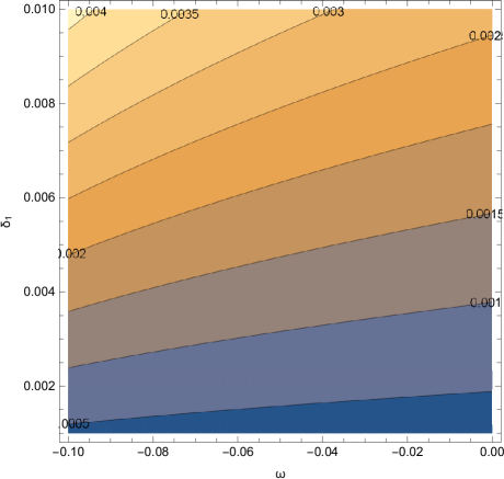
Figure 1: Tensor-to-scalar ratio $r$ depending on the parameters $\omega$ and exponent $\delta_{1}$ ranging from $[-0.01,-0.0001]$ and [0.001,0.01] respectively.

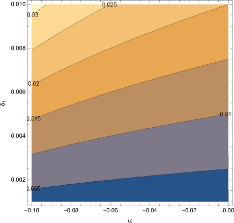
Figure 2: Field propagation velocity $c_{s}$ during the first horizon crossing depending on parameters $\omega$ and $\delta_{1}$ ranging from $[-0.01,-0.0001]$ and [0.001,0.01] respectively. It can easily be inferred that these values respect causality.

The model under study unfortunately should be rendered as intrinsically unrealistic. This is because $c_{s}=1.31198$ during the final stage of the inflationary era, which was not the case with the models studied in our previous works. In consequence, causality is violated and hence it is apparent that for some values of the free parameters, ghost degrees of freedom make their presence apparent. However, slight change in the numerical value of the non canonical kinetic term restores viability. This time, for $\omega=10^{-8}$ we have $n_{S}=0.966942$, $r=0.0264463$, $n_{T}=-0.0165289$ and $f_{NL}^{eq}=-5.68995$ while $c_{s}=0.2$ and $c_{s}=0.999998$ during the initial and final stage of the inflationary era respectively. In this case, causality is restored while the approximations assumed previously still apply. This is indicative of the fact that the free parameters of the theory must be chosen properly in certain cases in order to achieve compatibility. One should not naively designate the free parameters for even a slight detail as the one present in this paper, the sound speed at the end of the inflationary era, can turn the model into unrealistic. The behavior of the speed $c_{s}$ depending on various parameters can be found in Fig. 2. The only difference is the scalar potential. The same applies to the constant-roll case which shall be studied in the following section.

As a last comment, it would be wise to address the issue of the free parameters, and especially their range of values and the overall impact on the approximations made. In this first model, the only parameters that affect the results significantly are the ones showcased in the previous diagrams, namely the non canonical parameter $\omega$ and the exponent $\delta_{1}$ of the error function Gauss-Bonnet coupling. For the non canonical parameter $\omega$, it is essential to assume that its value is positive in this case in order to achieve a non superluminal velocity at the end of the inflationary era only, otherwise everything is in aggrement with the Planck 2018 data, whereas a negative value could still result in a viable $c_{s}$ only if $\delta$ is increased, however this is prohibited since $r$ becomes greater than 0.064 and thus cannot be accepted. A decisive factor as mentioned before is exponent $\delta_{1}$ which for greater values,for instance $\delta_{1}=-0.3$, the tensor-to-scalar ratio becomes equal to $r=0.07933$ which is obviously not an acceptable value. Moreover, such an increase results in a decrease in the equilateral nonlinear term to $f_{NL}^{eq}=-0.3332$. On the other hand, a decrease of the aforementioned exponent is acceptable since it decreases the tensor-to-scalar ratio and results in a rather significant increase on the amount of non Gaussianities. As an example, we mention that $\delta_{1}=-0.03$ generates an $f_{NL}^{eq}=-67.0681$ while the sound wave velocity during the initial and final stage remains real and below unity. Finally, the order of the Gauss-Bonnet coupling, namely the free parameter $\lambda_{1}$ is not so significant. It turns out that no observed index is dependent on it however it is worth mentioning that the sound speed at the final change can be altered from $\lambda_{1}$, only if it obtains a quite large value, for instance $\lambda_{1}\sim\mathcal{O}(10^{12})$ and beyond. Note however that an extreme value of $\mathcal{O}(10^{24})$ and greater would result in a direct violation of the approximations.

IV Einstein-Gauss-Bonnet $k$-Inflation Phenomenology with Constant-Roll Conditions

In the previous examples we showcased how the slow-roll assumptions facilitate our study greatly. In general, the fact that $\ddot{\phi}\ll H\dot{\phi}$ simplifies the continuity equation and an elegant analytic form for the scalar potential can be extracted. Another condition which has the same effect is the constant-roll evolution for the scalar field. This is a quite interesting case since in its core is a theory which can potentially produce non-Gaussianities in the primordial power spectrum, thus an enhanced equilateral non-linear term $f_{NL}^{eq}$ is naturally produced. Let us commence our study by introducing the constant-roll condition, that is $\ddot{\phi}=\beta H\dot{\phi}$ where $\beta$ is the constant-roll parameter. Essentially, from the previous results, it becomes apparent that $\epsilon_{2}=\beta$ hence we shall limit our work to only small values of $\beta$. From Eq. (3), one obtains the new time derivative for the scalar field, which is written as,

$$\centering\dot{\phi}=H\frac{(1-\beta)\xi^{\prime}}{\xi^{\prime\prime}}\,,\@add@centering$$ (34)

which as expected has the same limit as Eq. (4) for $\beta\to 0$. Consequently, the equations of motion are altered as follows,

$$\centering H^{2}\simeq\frac{\kappa^{2}V}{3},\,\@add@centering$$ (35)

$$\centering\dot{H}\simeq\kappa^{2}(\alpha X+\omega\gamma X^{\gamma}).\,\@add@centering$$ (36)

$$\centering V^{\prime}+H\dot{\phi}(\alpha(3+\beta)+\omega\gamma(\beta(2\gamma-1)+3)X^{\gamma-1})\simeq 0.\,\@add@centering$$ (37)

Since $\dot{\phi}$ is now proportional to $\beta$, both the scalar potential and the kinetic term are influenced, so typically equations (35)-(36) depend on $\beta$ even though it is not explicitly present. The rest auxiliary parameters and the slow-roll conditions as well, have the same forms as before however they also appear to depend on $\beta$. The only parameter which should be further amended, since it is of paramount importance in this particular formalism, is the $e$-folding number, which is essentially written in terms of the constant-roll parameter as,

$$\centering N=\frac{1}{1-\beta}\int_{\phi_{i}}^{\phi_{f}}{\frac{\xi^{\prime\prime}}{\xi^{\prime}}}\,,\@add@centering$$ (38)

IV.1 Revisiting the Error Function Model with the Constant-Roll Evolution

Let us now proceed with an example. Suppose that the Gauss-Bonnet coupling is once again an error function, for convenience since it simplifies the ratio $\xi^{\prime}/\xi^{\prime\prime}$. Let,

$$\centering\xi(\phi)=\frac{2\Lambda_{2}}{\sqrt{\pi}}\int_{0}^{\delta_{2}\kappa\phi}{e^{-x^{2}}dx}\,,\@add@centering$$ (39)

Then as a result, the scalar potential must have the following form in order for the continuity equation to be satisfied,

$$\centering V(\phi)=\frac{(2\delta_{2}^{2}\kappa\phi)^{2}\left(\alpha\left(\beta^{2}+2\beta-3\right)+12\delta_{2}^{2}\right)}{-(1-\beta)^{3}(\beta+1)\omega}\,,\@add@centering$$ (40)

which is simply a power-law potential with a constraint scalar amplitude. Essentially, even if the Gauss-Bonnet scalar coupling choice seems bizarre, the resulting scalar potential is elegant. In consequence, the slow-roll conditions along with the auxiliary parameters are now,

$$\centering\epsilon_{1}=-\frac{(1-\beta)^{2}\left((1-\beta)^{2}\omega V(\phi)-12\alpha\delta_{2}^{4}\kappa^{2}\phi^{2}\right)}{96\delta_{2}^{8}\kappa^{4}\phi^{4}}\,,\@add@centering$$ (41)

$$\centering\epsilon_{5}=\frac{4(\beta-1)\kappa^{3}\Lambda_{2}V(\phi)}{8(\beta-1)\kappa^{3}\Lambda_{2}V(\phi)-3\sqrt{\pi}\delta_{2}\phi e^{\delta_{2}^{2}\kappa^{2}\phi^{2}}}\,,\@add@centering$$ (42)

$$\centering\epsilon_{6}=-\frac{2(\beta-1)^{2}\kappa\Lambda_{2}\left(-\phi V^{\prime}(\phi)+2\delta_{2}^{2}\kappa^{2}\phi^{2}V(\phi)+V(\phi)\right)}{\delta_{2}^{2}\phi^{2}\left(8(\beta-1)\kappa^{3}\Lambda_{2}V(\phi)-3\sqrt{\pi}\delta_{2}\phi e^{\delta_{2}^{2}\kappa^{2}\phi^{2}}\right)}\,,\@add@centering$$ (43)

$$\centering\epsilon_{s}=\frac{4(1-\beta)\kappa^{3}\Lambda_{2}V(\phi)e^{-\delta_{2}^{2}\kappa^{2}\phi^{2}}}{3\sqrt{\pi}\delta_{2}\phi}-\frac{3\left(\frac{(1-\beta)^{4}\omega V(\phi)^{2}}{288\delta_{2}^{8}\kappa^{4}\phi^{4}}-\frac{\alpha(1-\beta)^{2}V(\phi)}{24\delta_{2}^{4}\kappa^{2}\phi^{2}}\right)}{V(\phi)}\,,\@add@centering$$ (44)

$$\centering\delta_{\xi}=\frac{(\beta-1)\kappa^{3}\Lambda_{2}V(\phi)e^{-\delta_{2}^{2}\kappa^{2}\phi^{2}}}{3\sqrt{\pi}\delta_{2}\phi}\,,\@add@centering$$ (45)

$$\centering\lambda=-\frac{(\beta-1)^{4}\omega V(\phi)^{2}}{288\delta_{2}^{8}\kappa^{4}\phi^{4}}\,,\@add@centering$$ (46)

Here we presented only a sample of the auxiliary parameters. From the simple form of index $\epsilon_{1}$, given that the potential is also a power-law, the final value of the scalar field of the inflationary era can be derived. Furthermore, since the Gauss-Bonnet coupling was chosen on purpose so as the ratio $\xi^{\prime}/\xi^{\prime\prime}$ is simplified, the initial value of the scalar field during the first horizon crossing is also derivable. The values of the scalar field for the case at hand are,

$$\centering\phi_{i}=\frac{\sqrt{\delta_{2}^{2}\kappa^{2}\phi_{f}^{2}+(1-\beta)N}}{\delta_{2}\kappa}\,,\@add@centering$$ (47)

$$\centering\phi_{f}=\pm\frac{\sqrt{1-\beta}\sqrt{-\alpha\beta^{2}+\alpha\beta+6\delta_{2}^{2}}}{\sqrt{12\beta\delta_{2}^{4}\kappa^{2}+12\delta_{2}^{4}\kappa^{2}}}\,,\@add@centering$$ (48)

Designating ($\omega$, $\alpha$, $\Lambda_{2}$, $\delta_{2}$, $N$, $\beta$)=(10, 1, 1, 0.4, 60, 0.001) produces compatible with the observations results as $n_{S}=0.966941$, $r=0.0135517$, $n_{T}=-0.0165296$ and $f_{NL}^{eq}=-22.8587$ are acceptable values. The non-Gaussianities are obviously enhanced, since $f_{NL}^{eq}=-22.8587$ in this case. Furthermore, the field propagation velocity in the initial and final stage has the numerical values of $c_{s}=0.102481$ and $c_{s}=0.100141$ respectively, which suggests a decrease but more importantly predicts no Jeans instabilities, hence the model is free of ghosts. The behavior of the inflationary phenomenology parameters and of the sound wave speed can be found in Figs. 3 and 4, for various sets of values of the free parameters. The slow-roll indices obtain the values $\epsilon_{1}=0.0082648$, $\epsilon_{5}=\epsilon_{6}=2\cdot 10^{-27}$ which is practically zero and moreover the auxiliary slow-varying parameters are $\delta_{\xi}=-5\cdot 10^{-28}$, $s=5\cdot 10^{-18}$, $\eta_{s}=0.0165289$ and $\lambda=-0.00645602$. It should be noted here that even though $\beta\ll 1$, the overall phenomenology is quite different between the slow-roll and constant-roll cases, something that can easily be ascertained from the numerical values of the auxiliary parameters, for instance the field propagation velocity. A notable feature of the model is that $f_{NL}^{eq}$ is quite large, thus the primordial power spectrum of this model has enhanced non-Gaussianities, and actually to a large magnitude. This is also the main difference between the canonical and $k$-inflation-corrected models.

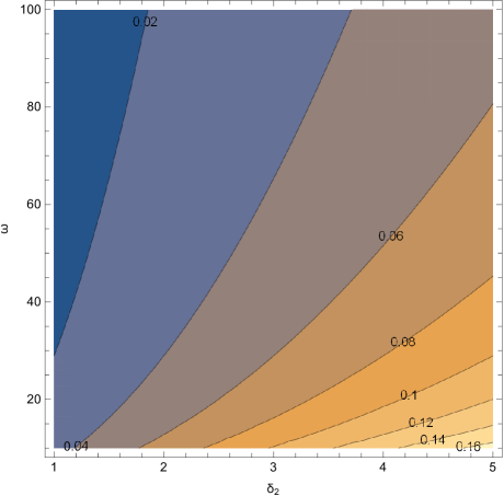
Figure 3: Tensor-to-scalar ratio $r$ depending on the non canonical parameter $\omega$ and exponent $\delta_{2}$ ranging from $[10,100]$ and [1,5] respectively. Apart from the acceptable values, it is clear that there exists also pairs which produce incompatible with the observations tensor-to-scalar ratio.

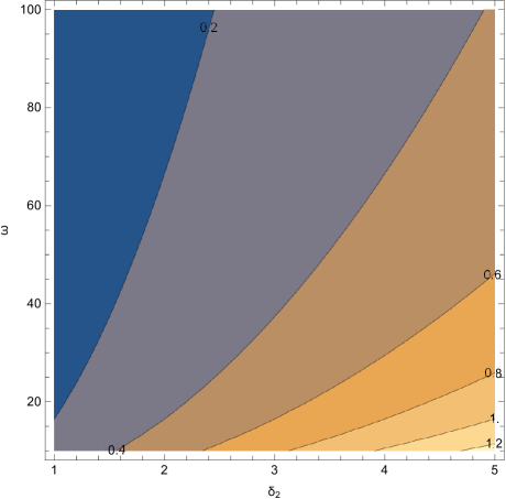
Figure 4: Field propagation velocity $c_{s}$ during the first horizon crossing depending on parameters $\omega$ and $\delta_{2}$ ranging from $[10,100]$ and [1,5] respectively. For certain pairs, the resulting velocity is greater than unity, meaning causality is violated and hence are unacceptable. Moreover, these pairs also produce an unacceptable value for the tensor-to-scalar ratio so they are also excluded from an observation perspective.

When it comes to the parameter $\alpha$, we mention that during the first horizon crossing, either values $\alpha=-1,0$ are capable of producing viable results but during the final stage, the field velocity becomes complex, therefore with this approach, $\alpha$ gives rise to ghosts. Exponent $\delta_{2}$ affects the results, in particular increasing its value results in a decrease to the tensor-to-scalar ratio and a subsequent increase to the equilateral non-linear term, while the scalar spectral index remains invariant. The constant-roll parameter on the other hand affects only the scalar spectral index $n_{S}$ and the amount of non-Gaussianities, meaning $f_{NL}^{eq}$. Essentially, increasing $\beta$ leads to a subsequent increase in $n_{S}$ while it lowers the value of $f_{NL}^{eq}$. Finally, $\omega$ influences only the tensor-to-scalar ratio and the equilateral non-linear term. Decreasing its order of magnitude leads to an enhanced $f_{NL}^{eq}$ while it decreases $r$. Also, $\omega$ must be negative in order to avoid the emergence of ghosts. Finally, for the approximations made, we mention that $\dot{H}/H^{2}\sim\mathcal{O}(10^{-3})$, $\alpha X+\omega X^{\gamma}\sim\mathcal{O}(10^{-2})$ and $V\sim\mathcal{O}(1)$. Furthermore, $24\dot{\xi}H^{3}\sim\mathcal{O}(10^{-26})$, $16\dot{\xi}H\dot{H}\sim\mathcal{O}(10^{-28})$ and $24\xi^{\prime}H^{4}\sim\mathcal{O}(10^{-25})$ while $V^{\prime}\sim\mathcal{O}(10^{-1})$, hence all the approximations indeed apply.

As in the slow-roll case, let us examine the impact of the free parameters on the observed indices and the sound wave velocity. As shown in Figs. 3 and 4, $\delta_{2}$ and $\omega$ are once again the decisive factors on $r$ and $c_{s}$. Furthermore, the Gauss-Bonnet dimensionless parameter, $\lambda_{2}$ in this case, does not influence the results, apart from the sound wave velocity during the ending stage on inflation and once again only by extreme values. It stands to reason that the two model have similar dependencies on $\omega$ and $\delta_{2}$. The new addition, the constant-roll parameter seems to be quite interesting. Here, $\beta$is not prohibited to obtain large values, in fact $\beta=0.2$ for instance seems to produce results which are in agreement with recent observations, as $n_{S}=0.9674$, $r=0.01472$ and $f_{NL}=-18.2796$. Here, the amount of non Gaussianities is decreased, and no violation of causality is observed neither during the first horizon crossing not the end of the inflationary era. For larger values of the constant-roll parameter, the scalar spectral index passes the threshold and no longer resides in the area of acceptance. This is also one of the reasons a small value for the constant-roll parameter was chosen in the first place, so as to achieve compatibility for $n_{S}$, enhance $f_{NL}^{eq}$ and obtain a slow-roll index $\epsilon_{2}$ of order $\mathcal{O}(10^{-3})$, meaning a small value as the rest slow-roll indices. The opposite applies when the constant-roll parameter is negative and therefore, $\beta=-0.3$ can enhance further the non Gaussianities and produce viable sound wave velocities but the scalar spectral index is once again outside of the bound. Thus, compatibility can indeed be achieved with the Planck 2018 collaboration once the constant-roll parameter is roughly of order $\mathcal{O}(10^{-1})$ and below.

Similar to the previous case, the value of $\gamma=-1$ is more than capable of producing compatible with the observations results while simultaneously being free of ghosts. Also, between the slow-roll and constant-roll evolution, there exists no significant difference in the case on non-Gaussianities. Lastly, the reader should not be discouraged and think that this formalism works only under the error function Gauss-Bonnet coupling. In principle, there exists no limitation however the error function is quite convenient given that the ratio $\xi^{\prime}/\xi^{\prime\prime}$ appears in our calculations. Other couplings such as a power-law and an exponential should also work.

V Conclusions

Studying the dynamics of an Einstein-Gauss-Bonnet gravity accompanied by a non-canonical kinetic term during the inflationary era has revealed many interesting features. Firstly, the realization that the gravitational waves propagate through spacetime with the velocity of light, makes it abundantly clear that the scalar functions of the theory, in this case the scalar potential and the Gauss-Bonnet coupling, are interconnected, or in other words cannot be freely designated. Furthermore, the kinetic term is strongly dependent on the Gauss-Bonnet coupling, meaning that the non-canonical kinetic part is itself interconnected with string corrections. In this paper, we showed that the $k$-inflation-corrected Einstein-Gauss-Bonnet gravity, under both the slow-roll and constant-roll conditions, is capable of producing viable phenomenology since the observational quantities are compatible with the latest observations coming from the Planck 2018 data. Since a non-canonical kinetic term is present, the amount of non-Gaussianities, as expected, is enhanced but still resides in the area of acceptance. The only obstacle is this framework is the field propagation velocity $c_{s}$ which can lead to Jeans instabilities or superluminal velocities. As demonstrated, the choice of a quadratic kinetic term is capable of producing a ghost free model without violating causality, by choosing appropriately the values of the free parameters. Moreover, certain models may seem to lead to viable phenomenology. Finally, we mention that the slow-roll approach for the scalar field is not mandatory and in fact the constant-roll assumption is also an option capable for producing viable results. Undoubtedly, the same principles are expected to apply in the case of a non-minimal coupling between the Ricci scalar and the scalar field. Finally, an important outcome of this work is that the primordial non-Gaussianities in the power spectrum, are enhanced in the presence of the $k$-inflation corrections, for both the constant and slow-roll conditions. The magnitude of the equilateral momentum non-linear term $f_{NL}^{eq}$ in the constant-roll case, is reportable and quite large in magnitude.

References

- (1) A. H. Guth, Phys. Rev. D 23 (1981) 347. doi:10.1103/PhysRevD.23.347
- (2) A. D. Linde, Phys. Rev. D 49 (1994) 748 doi:10.1103/PhysRevD.49.748 [astro-ph/9307002].
- (3) A. D. Linde, Phys. Lett. 129B (1983) 177. doi:10.1016/0370-2693(83)90837-7
- (4) S. Nojiri, S. D. Odintsov and V. K. Oikonomou, Phys. Rept. 692 (2017) 1 doi:10.1016/j.physrep.2017.06.001 [arXiv:1705.11098 [gr-qc]].
- (5) S. Nojiri and S. D. Odintsov, Phys. Rept. 505 (2011) 59 doi:10.1016/j.physrep.2011.04.001 [arXiv:1011.0544 [gr-qc]].
- (6) S. Nojiri and S. D. Odintsov, eConf C 0602061 (2006) 06 [Int. J. Geom. Meth. Mod. Phys. 4 (2007) 115] doi:10.1142/S0219887807001928 [hep-th/0601213].
- (7) S. Capozziello and M. De Laurentis, Phys. Rept. 509 (2011) 167 doi:10.1016/j.physrep.2011.09.003 [arXiv:1108.6266 [gr-qc]].
- (8) V. Faraoni and S. Capozziello, Fundam. Theor. Phys. 170 (2010). doi:10.1007/978-94-007-0165-6
- (9) G. J. Olmo, Int. J. Mod. Phys. D 20 (2011) 413 doi:10.1142/S0218271811018925 [arXiv:1101.3864 [gr-qc]].
- (10) S. Nojiri and S. D. Odintsov, Phys. Rev. D 68 (2003), 123512 doi:10.1103/PhysRevD.68.123512 [arXiv:hep-th/0307288 [hep-th]].
- (11) S. D. Odintsov and V. K. Oikonomou, EPL 129 (2020) no.4, 40001 doi:10.1209/0295-5075/129/40001 [arXiv:2003.06671 [gr-qc]].
- (12) S. D. Odintsov and V. K. Oikonomou, Phys. Rev. D 101 (2020) no.4, 044009 doi:10.1103/PhysRevD.101.044009 [arXiv:2001.06830 [gr-qc]].
- (13) P. M. Sa, Universe 6 (2020) no.6, 78 [arXiv:2002.09446 [gr-qc]].
-
(14)
R. Brandenberger and P. Peter,
Found. Phys. 47 (2017) no.6, 797
doi:10.1007/s10701-016-0057-0
[arXiv:1603.05834 [hep-th]].;
J. de Haro and Y. F. Cai, Gen. Rel. Grav. 47 (2015) no.8, 95 doi:10.1007/s10714-015-1936-y [arXiv:1502.03230 [gr-qc]].;
Y. F. Cai, Sci. China Phys. Mech. Astron. 57 (2014) 1414 doi:10.1007/s11433-014-5512-3 [arXiv:1405.1369 [hep-th]]. - (15) J. c. Hwang and H. Noh, Phys. Rev. D 71 (2005) 063536 doi:10.1103/PhysRevD.71.063536 [gr-qc/0412126].
- (16) S. Nojiri, S. D. Odintsov and M. Sami, Phys. Rev. D 74 (2006) 046004 doi:10.1103/PhysRevD.74.046004 [hep-th/0605039].
- (17) G. Cognola, E. Elizalde, S. Nojiri, S. Odintsov and S. Zerbini, Phys. Rev. D 75 (2007) 086002 doi:10.1103/PhysRevD.75.086002 [hep-th/0611198].
- (18) S. Nojiri, S. D. Odintsov and M. Sasaki, Phys. Rev. D 71 (2005) 123509 doi:10.1103/PhysRevD.71.123509 [hep-th/0504052].
- (19) S. Nojiri and S. D. Odintsov, Phys. Lett. B 631 (2005) 1 doi:10.1016/j.physletb.2005.10.010 [hep-th/0508049].
- (20) M. Satoh, S. Kanno and J. Soda, Phys. Rev. D 77 (2008) 023526 doi:10.1103/PhysRevD.77.023526 [arXiv:0706.3585 [astro-ph]].
- (21) K. Bamba, A. N. Makarenko, A. N. Myagky and S. D. Odintsov, JCAP 1504 (2015) 001 doi:10.1088/1475-7516/2015/04/001 [arXiv:1411.3852 [hep-th]].
- (22) Z. Yi, Y. Gong and M. Sabir, Phys. Rev. D 98 (2018) no.8, 083521 doi:10.1103/PhysRevD.98.083521 [arXiv:1804.09116 [gr-qc]].
- (23) Z. K. Guo and D. J. Schwarz, Phys. Rev. D 80 (2009) 063523 doi:10.1103/PhysRevD.80.063523 [arXiv:0907.0427 [hep-th]].
- (24) Z. K. Guo and D. J. Schwarz, Phys. Rev. D 81 (2010) 123520 doi:10.1103/PhysRevD.81.123520 [arXiv:1001.1897 [hep-th]].
- (25) P. X. Jiang, J. W. Hu and Z. K. Guo, Phys. Rev. D 88 (2013) 123508 doi:10.1103/PhysRevD.88.123508 [arXiv:1310.5579 [hep-th]].
- (26) P. Kanti, R. Gannouji and N. Dadhich, Phys. Rev. D 92 (2015) no.4, 041302 doi:10.1103/PhysRevD.92.041302 [arXiv:1503.01579 [hep-th]].
- (27) C. van de Bruck, K. Dimopoulos, C. Longden and C. Owen, arXiv:1707.06839 [astro-ph.CO].
- (28) P. Kanti, J. Rizos and K. Tamvakis, Phys. Rev. D 59 (1999) 083512 doi:10.1103/PhysRevD.59.083512 [gr-qc/9806085].
- (29) E. O. Pozdeeva, M. R. Gangopadhyay, M. Sami, A. V. Toporensky and S. Y. Vernov, arXiv:2006.08027 [gr-qc].
- (30) I. Fomin, arXiv:2004.08065 [gr-qc].
- (31) M. De Laurentis, M. Paolella and S. Capozziello, Phys. Rev. D 91 (2015) no.8, 083531 doi:10.1103/PhysRevD.91.083531 [arXiv:1503.04659 [gr-qc]].
- (32) S. Chervon, I. Fomin, V. Yurov and A. Yurov, doi:10.1142/11405
- (33) K. Nozari and N. Rashidi, Phys. Rev. D 95 (2017) no.12, 123518 doi:10.1103/PhysRevD.95.123518 [arXiv:1705.02617 [astro-ph.CO]].
- (34) S. D. Odintsov and V. K. Oikonomou, Phys. Rev. D 98 (2018) no.4, 044039 doi:10.1103/PhysRevD.98.044039 [arXiv:1808.05045 [gr-qc]].
- (35) S. Kawai, M. a. Sakagami and J. Soda, Phys. Lett. B 437, 284 (1998) doi:10.1016/S0370-2693(98)00925-3 [gr-qc/9802033].
- (36) Z. Yi and Y. Gong, Universe 5 (2019) no.9, 200 doi:10.3390/universe5090200 [arXiv:1811.01625 [gr-qc]].
- (37) C. van de Bruck, K. Dimopoulos and C. Longden, Phys. Rev. D 94 (2016) no.2, 023506 doi:10.1103/PhysRevD.94.023506 [arXiv:1605.06350 [astro-ph.CO]].
- (38) B. Kleihaus, J. Kunz and P. Kanti, arXiv:1910.02121 [gr-qc].
- (39) A. Bakopoulos, P. Kanti and N. Pappas, Phys. Rev. D 101 (2020) no.4, 044026 doi:10.1103/PhysRevD.101.044026 [arXiv:1910.14637 [hep-th]].
- (40) K. i. Maeda, N. Ohta and R. Wakebe, Eur. Phys. J. C 72 (2012) 1949 doi:10.1140/epjc/s10052-012-1949-6 [arXiv:1111.3251 [hep-th]].
- (41) A. Bakopoulos, P. Kanti and N. Pappas, arXiv:2003.02473 [hep-th].
- (42) W. Ai, [arXiv:2004.02858 [gr-qc]].
- (43) S. D. Odintsov and V. K. Oikonomou, Phys. Lett. B 797 (2019) 134874 doi:10.1016/j.physletb.2019.134874 [arXiv:1908.07555 [gr-qc]].
- (44) V. K. Oikonomou and F. P. Fronimos, [arXiv:2007.11915 [gr-qc]].
- (45) S. D. Odintsov, V. K. Oikonomou and F. P. Fronimos, Annals Phys. 420 (2020), 168250 doi:10.1016/j.aop.2020.168250 [arXiv:2007.02309 [gr-qc]].
- (46) V. K. Oikonomou and F. P. Fronimos, [arXiv:2006.05512 [gr-qc]].
- (47) S. D. Odintsov and V. K. Oikonomou, Phys. Lett. B 805 (2020), 135437 doi:10.1016/j.physletb.2020.135437 [arXiv:2004.00479 [gr-qc]].
- (48) S. D. Odintsov, V. K. Oikonomou and F. P. Fronimos, [arXiv:2003.13724 [gr-qc]].
- (49) S. D. Odintsov, V. K. Oikonomou, F. P. Fronimos and S. A. Venikoudis, Phys. Dark Univ. 30 (2020), 100718 doi:10.1016/j.dark.2020.100718 [arXiv:2009.06113 [gr-qc]].
- (50) R. Easther and K. i. Maeda, Phys. Rev. D 54 (1996) 7252 doi:10.1103/PhysRevD.54.7252 [hep-th/9605173].
- (51) I. Antoniadis, J. Rizos and K. Tamvakis, Nucl. Phys. B 415 (1994) 497 doi:10.1016/0550-3213(94)90120-1 [hep-th/9305025].
- (52) I. Antoniadis, C. Bachas, J. R. Ellis and D. V. Nanopoulos, Phys. Lett. B 257 (1991), 278-284 doi:10.1016/0370-2693(91)91893-Z
- (53) P. Kanti, N. Mavromatos, J. Rizos, K. Tamvakis and E. Winstanley, Phys. Rev. D 54 (1996), 5049-5058 doi:10.1103/PhysRevD.54.5049 [arXiv:hep-th/9511071 [hep-th]].
- (54) P. Kanti, N. Mavromatos, J. Rizos, K. Tamvakis and E. Winstanley, Phys. Rev. D 57 (1998), 6255-6264 doi:10.1103/PhysRevD.57.6255 [arXiv:hep-th/9703192 [hep-th]].
- (55) B. P. Abbott et al. “Multi-messenger Observations of a Binary Neutron Star Merger,” Astrophys. J. 848 (2017) no.2, L12 doi:10.3847/2041-8213/aa91c9 [arXiv:1710.05833 [astro-ph.HE]].
- (56) J. M. Ezquiaga and M. Zumalacarregui, Phys. Rev. Lett. 119 (2017) no.25, 251304 doi:10.1103/PhysRevLett.119.251304 [arXiv:1710.05901 [astro-ph.CO]].
- (57) C. Armendariz-Picon, T. Damour and V. F. Mukhanov, Phys. Lett. B 458 (1999) 209 doi:10.1016/S0370-2693(99)00603-6 [hep-th/9904075].
- (58) T. Chiba, T. Okabe and M. Yamaguchi, Phys. Rev. D 62 (2000) 023511 doi:10.1103/PhysRevD.62.023511 [astro-ph/9912463].
- (59) C. Armendariz-Picon, V. F. Mukhanov and P. J. Steinhardt, Phys. Rev. Lett. 85 (2000) 4438 doi:10.1103/PhysRevLett.85.4438 [astro-ph/0004134].
- (60) J. Matsumoto and S. Nojiri, Phys. Lett. B 687 (2010) 236 doi:10.1016/j.physletb.2010.03.030 [arXiv:1001.0220 [hep-th]].
- (61) C. Armendariz-Picon, V. F. Mukhanov and P. J. Steinhardt, Phys. Rev. D 63 (2001) 103510 doi:10.1103/PhysRevD.63.103510 [astro-ph/0006373].
- (62) T. Chiba, Phys. Rev. D 66 (2002) 063514 doi:10.1103/PhysRevD.66.063514 [astro-ph/0206298].
- (63) M. Malquarti, E. J. Copeland, A. R. Liddle and M. Trodden, Phys. Rev. D 67 (2003) 123503 doi:10.1103/PhysRevD.67.123503 [astro-ph/0302279].
- (64) M. Malquarti, E. J. Copeland and A. R. Liddle, Phys. Rev. D 68 (2003) 023512 doi:10.1103/PhysRevD.68.023512 [astro-ph/0304277].
- (65) L. P. Chimento and A. Feinstein, Mod. Phys. Lett. A 19 (2004) 761 doi:10.1142/S0217732304013507 [astro-ph/0305007].
- (66) L. P. Chimento, Phys. Rev. D 69 (2004) 123517 doi:10.1103/PhysRevD.69.123517 [astro-ph/0311613].
- (67) R. J. Scherrer, Phys. Rev. Lett. 93 (2004) 011301 doi:10.1103/PhysRevLett.93.011301 [astro-ph/0402316].
- (68) J. M. Aguirregabiria, L. P. Chimento and R. Lazkoz, Phys. Rev. D 70 (2004) 023509 doi:10.1103/PhysRevD.70.023509 [astro-ph/0403157].
- (69) C. Armendariz-Picon and E. A. Lim, JCAP 0508 (2005) 007 doi:10.1088/1475-7516/2005/08/007 [astro-ph/0505207].
- (70) L. R. Abramo and N. Pinto-Neto, Phys. Rev. D 73 (2006) 063522 doi:10.1103/PhysRevD.73.063522 [astro-ph/0511562].
- (71) A. D. Rendall, Class. Quant. Grav. 23 (2006) 1557 doi:10.1088/0264-9381/23/5/008 [gr-qc/0511158].
- (72) J. P. Bruneton, Phys. Rev. D 75 (2007) 085013 doi:10.1103/PhysRevD.75.085013 [gr-qc/0607055].
- (73) R. de Putter and E. V. Linder, Astropart. Phys. 28 (2007) 263 doi:10.1016/j.astropartphys.2007.05.011 [arXiv:0705.0400 [astro-ph]].
- (74) E. Babichev, V. Mukhanov and A. Vikman, JHEP 0802 (2008) 101 doi:10.1088/1126-6708/2008/02/101 [arXiv:0708.0561 [hep-th]].
- (75) C. Deffayet, X. Gao, D. A. Steer and G. Zahariade, Phys. Rev. D 84 (2011) 064039 doi:10.1103/PhysRevD.84.064039 [arXiv:1103.3260 [hep-th]].
- (76) N. Kan, K. Shiraishi and M. Yashiki, arXiv:1811.11967 [gr-qc].
- (77) S. Unnikrishnan, V. Sahni and A. Toporensky, JCAP 1208 (2012) 018 doi:10.1088/1475-7516/2012/08/018 [arXiv:1205.0786 [astro-ph.CO]].
- (78) S. Li and A. R. Liddle, JCAP 1210 (2012) 011 doi:10.1088/1475-7516/2012/10/011 [arXiv:1204.6214 [astro-ph.CO]].
- (79) A. De Felice and S. Tsujikawa, JCAP 1104 (2011) 029 doi:10.1088/1475-7516/2011/04/029 [arXiv:1103.1172 [astro-ph.CO]].
- (80) Y. Akrami et al. [Planck Collaboration], arXiv:1807.06211 [astro-ph.CO].