An a posteriori strategy for adaptive schemes in time and space

Abstract

A nonlinear adaptive procedure for optimising both the schemes in time and space is proposed in view of increasing the numerical efficiency and reducing the computational time. The method is based on a four-parameter family of schemes we shall tune in function of the physical data (velocity, diffusion), the characteristic size in time and space, and the local regularity of the function leading to a nonlinear procedure. The a posteriori strategy we adopt consists in, given the solution at time $t^{n}$, computing a candidate solution with the highest accurate schemes in time and space for all the nodes. Then, for the nodes that present some instabilities, both the schemes in time and space are modified and adapted in order to preserve the stability with a large time step. The updated solution is computed with node-dependent schemes both in time and space. For the sake of simplicity, only convection-diffusion problems are addressed as a prototype with a two-parameters five-points finite difference method for the spatial discretisation together with an explicit time two-parameters four-stages Runge-Kutta method. We prove that we manage to obtain an optimal time-step algorithm that produces accurate numerical approximations exempt of non-physical oscillations.

1 Introduction

High order discrete schemes for equations involving hyperbolic operators are likely to produce non physical oscillations. Even for linear problems, a nonlinear routine is mandatory to control the over- and under-shooting in the vicinity of points where the solution presents large gradients. Technologies such as MUSCL or WENO [19, 20], among the most popular, have been developed for half a century and manage to efficiently reduce or eliminate the numerical instabilities, namely to avoid the oscillations near the discontinuities and the extrema points. More specifically, for the convection-diffusion problems, different approaches have been considered: variable-order non-oscillatory scheme (VONOS), hybrid-linear parabolic approximation (HLPA), sharp and monotonic algorithm for realistic transport (SMART), weighted-average coefficient ensuring boundedness (WACEB), convergent and universally bounded interpolation scheme for the treatment of advection (CUBISTA) and an adaptive bounded version of the QUICK with estimated streaming terms (QUICKEST) called ADBQUICKEST (see references for these methods in [12]). The numerical solution obtained with these schemes is at least second-order accurate in regions where the solution is smooth enough but retains the first-order approximation in regions where the solution presents large gradients for the sake of stability.

All the stabilisation procedures mainly address the scheme in space whereas the scheme in time is merely discretised with a Runge-Kuta (RK) method or its Strong Stability Preserving (SSP) version [26, 27]. Very little attention has been paid on the time discretisation and a nonlinear dynamical procedure for optimising both the schemes in time and space is desirable to increase the numerical efficiency. Several traditional numerical methods were revisited in order to articulate space and time schemes together, aiming to increase the allowable time step. Bourchtein [5] constructed an explicit central difference method of second order applied to the one- and two-dimensional advection equations based on the generalised leap-frog type method with the main goal of increasing the allowable time step, with some deterioration in the accuracy of the solution. Chadha and Madden [7] consider the numerical solution of a linear time dependent advection–diffusion problem by an implicit two-weight, three-point central finite difference scheme. They extend the scheme proposed by them in [8], to incorporate an optimal time step selection algorithm for the method. The resulting method, based on optimal values of weights and optimal time-stepping, is of fifth-order in space, and third-order in time.

Other numerical schemes are based on prediction-correction techniques [25]. In [4], the authors present an adaptive finite element scheme for the advection-reaction-diffusion equation based on a stabilized finite element method combined with a residual error estimator. The adaptive process corrects the meshes allowing to capture boundary and inner layers very sharply and without significant oscillations. In [17], the authors have developed some a posteriori error estimates using a stabilized scheme combined with a shock-capturing technique to control the local oscillations in the crosswind direction. In [28], the author has introduced an error estimate for the advection–diffusion equation based on the solution of local problems on each element of the triangulation. Artificial compression method (ACM) based filter scheme is also investigated in [29]. The spatially fourth-order (or higher non-dissipative) scheme in space is used at all times but additional numerical dissipation is made at the shock layers to control the stability.

In the last decade, the a posteriori paradigm has been developed to prevent the numerical solution from creating non physical oscillations: the so-called Multidimensional Optimal Order Detection Method (MOOD) method [9, 10]. The principle consists in building a candidate solution with the highest order scheme in space. Then the guess solution admissibility is analysed using detectors to check some physical properties of non physical oscillations. The nodes that present non-compliance’s solution are tagged and the numerical scheme is only altered for that points by reducing the scheme order (basically adding more viscosity or reducing the polynomial reconstruction degree). The numerical approximation for the cured nodes and their neighbours is computed again to eliminate the oscillations. The goal of this the paper is the design of an adaptive technique, based on the a posteriori paradigm, to provide the optimal choice of the time and space schemes, that enables to compute a stable solution with the largest time step.

To present our strategy, we deal with the one-dimension linear convection-diffusion problem since all the important ingredients are already addressed in this simple scalar equation and enable to highlight the connections between the scheme in time and the scheme in space. Notice that, even a linear problem requires a nonlinear routine for stabilisation when dealing with rough solutions and the convection-diffusion equation involves the two main operator in simulations. For the sake of simplicity, we only consider two schemes in space and two schemes in time with very different characteristics and we aim to optimise the space accuracy and the time step to produce physically admissible numerical solutions with no spurious oscillations.

The crucial point lies on the confrontation between the discretisations in space and time: the eigenvalues associated to the space scheme have to fit into the stability domain of the RK scheme. Several parameters play a major role in the trade-off between accuracy and stability. On the one hand, the scheme in space together with the Péclet number determine the eigenvalues distribution in the complex plane. On the other hand, the RK scheme stability region and the accuracy is characterised by the Butcher tableau [6]. At last, the stability condition between the two schemes is controlled by the Courant–Friedrichs–Lewy (CFL) condition depending on the time discretisation parameter $\Delta t$.

In this study, we consider a two-parameter family of finite difference schemes in space that characterise the spectrum and the accuracy. Similarly, the time discretization is a two-parameter family of schemes by considering a four-stage RK method where we impose to be at least second-order. The global method is a four-parameter family of schemes we shall tune in function of the physical data (velocity, diffusion), the characteristic size in time and space, and the local regularity of the function leading to a nonlinear procedure since the scheme depends on the approximation itself.

The design of the schemes in space has to respect some basic principles in order to produce an eligible blending. First we only consider five-point finite difference methods involving the same centred stencil but the coefficients are node dependent. Similarly the four-stage RK scheme is also node dependent and it is mandatory that the four sub-steps are the same for all the nodes for the sake of compatibility leading to some additional constraints in the design of the Butcher’s tableau. The a posteriori strategy we adopt consists in, given the solution at time $t^{n}$, computing a candidate solution with the highest accurate scheme in time and space for all the nodes. Then applying the detectors, we determine the nodes to be corrected and switch the scheme in space. Unfortunately, it usually leads to a reduction of the local time step for the sake of stability. To overcome such a problem and preserve a large time step, we may have to switch the time scheme. We then obtain, the optimal combination of time and space schemes for each node and iteration while we use the common time step to update the solution.

The organisation of the paper is the following. We briefly present in Section 2 the spectral analysis of the five-point finite difference method focusing on the spectral curves description with respect to the two free parameters. Section 3 is dedicated to the four-stage RK method where we analyse the impact of the two free parameters on the stability region. The stability of the time and space schemes combination is carried out in Section 4 where we determine the optimal time step for each scenario. Finally, Section 5 presents our a posteriori method to design a node by node optimal scheme both in time and space. At last in Section 6 conclusions and perspectives are drawn.

2 Discrete convection-diffusion operator analysis

This section is dedicated to the spectrum of the discrete convection-diffusion operator we shall use in our stability analysis. Let $\phi=\phi(x)$ be a smooth 1-periodic function defined in $\mathbb{R}$, i.e., $\phi(x+1)=\phi(x)$. We define the convection-diffusion operator

$$\mathfrak{E}[\phi]=-u\phi^{\prime}+\kappa\phi^{\prime\prime},$$ (1)

where $u\geq 0$ and $\kappa\geq 0$ are the convective and diffusive coefficients, respectively. We restrict the study case to the bounded domain $[0,1]$ by applying a periodic condition. Let $I\in\mathbb{N}$ and $\Delta x=1/I$. We denote $x_{i}=i\Delta x$, $i\in\mathbb{Z}$, a uniform discretisation of the real axis and set $\Psi=(\psi_{i})_{i\in\mathbb{Z}}$ a vector with an infinite number of real value entries. Periodicity yields $\psi_{i+I}=\psi_{i}$, for all $i\in\mathbb{Z}$, hence the relevant data is only given by components $\psi_{i}$, $i=1,\ldots,I$. We shall use the same notation $\Psi=(\psi_{i})_{i=1}^{I}$ to denote both the whole vector and its finite representation, being the other components given by periodicity.

2.1 Five-point discrete schemes

A generic conservative five-point numerical scheme is defined by an ordered list of 5 coefficients which we indicate with

$$E=(a_{-2},a_{-1},a_{0},a_{1},a_{2}),\quad a_{j}\in\mathbb{R},j=-2,\ldots,2,$$ (2)

where the coefficients satisfy the null summation constraint for the sake of conservation

$$a_{-2}+a_{-1}+a_{0}+a_{1}+a_{2}=0.$$

For any $I$-periodic vector $\Psi=(\psi_{i})_{i\in\mathbb{Z}}$, the $E$-scheme applied to $\Psi$ provides the vector $E\Psi$ given component-wise by

$$(E\Psi)_{i}=a_{-2}\psi_{i-2}+a_{-1}\psi_{i-1}+a_{0}\psi_{i}+a_{1}\psi_{i+1}+a_{2}\psi_{i+2},\quad i\in\mathbb{Z}.$$

Periodicity of $\Psi$ yields that $E\Psi$ also satisfies the periodicity property hence the finite vector representation $E\Psi=((E\Psi)_{i})_{i=1}^{I}$ completely describes the whole vector. We highlight the four particular cases

$$E_{1}=\mathopen{}\mathclose{{}\left(\frac{1}{12},-\frac{2}{3},0,\frac{2}{3},-\frac{1}{12}}\right),\qquad E_{2}=\mathopen{}\mathclose{{}\left(-\frac{1}{12},\frac{4}{3},-\frac{5}{2},\frac{4}{3},-\frac{1}{12}}\right),$$

$$E_{3}=\mathopen{}\mathclose{{}\left(-\frac{1}{2},1,0,-1,\frac{1}{2}}\right), E_{4}=\mathopen{}\mathclose{{}\left(1,-4,6,-4,1}\right),$$

that provide approximations for the first-, second-, third-, and fourth-order derivatives, respectively. Denoting $\Psi=(\phi(x_{i}))_{i\in\mathbb{Z}}$ for any regular $1$-periodic function $\phi=\phi(x)$, consistency errors read

$$(E_{1}\Psi)_{i}=\phi^{(1)}(x_{i})+\mathcal{O}(\Delta x^{4}),\qquad (E_{2}\Psi)_{i}=\phi^{(2)}(x_{i})+\mathcal{O}(\Delta x^{4}),$$

$$(E_{3}\Psi)_{i}=\phi^{(3)}(x_{i})+\mathcal{O}(\Delta x^{2}), (E_{4}\Psi)_{i}=\phi^{(4)}(x_{i})+\mathcal{O}(\Delta x^{2}).$$

The fourth-order five-point discretisation of operator (1) is given by the optimal combination

$$E=-\frac{u}{\Delta x}\mathopen{}\mathclose{{}\left(E_{1}-\frac{E_{2}}{Pe}}\right),$$

where $Pe=\frac{u\,\Delta x}{\kappa}$ represents the cell Péclet number. Instabilities may appear and one has to damp the oscillations by using third- and fourth-derivative approximations. To this end, we consider more general five-point conservative schemes of the form

$$E=E(\theta_{3},\theta_{4},Pe)=-\frac{u}{\Delta x}\mathopen{}\mathclose{{}\left(E_{1}-\frac{E_{2}}{Pe}+\theta_{3}E_{3}+\theta_{4}E_{4}}\right),$$ (3)

parameterised by $\theta_{3},\theta_{4}\in\mathbb{R}$, and $Pe$. Substituting the expressions of $E_{1}$, $E_{2}$, $E_{3}$, and $E_{4}$, scheme $E$ reads

$$E(\theta_{3},\theta_{4},Pe)=-\frac{u}{\Delta x}\mathopen{}\mathclose{{}\left(\frac{(12\theta_{4}-6\theta_{3}+1)Pe+1}{12Pe},-\frac{(12\theta_{4}-3\theta_{3}+2)Pe+4}{3Pe},}\right.\\ \mathopen{}\mathclose{{}\left.\frac{12\theta_{4}Pe+5}{2Pe},-\frac{(12\theta_{4}+3\theta_{3}-2)Pe+4}{3Pe},\frac{(12\theta_{4}+6\theta_{3}-1)Pe+1}{12Pe}}\right).$$ (4)

Remark 1

If $u=0$ and $\kappa\neq 0$ (pure diffusive problem), $Pe=0$ and expression (4) should be rewritten specifically for $u=0$ taking into account $\theta_{3}$ and $\theta_{4}$. If $\kappa=0$ and $u\neq 0$ (pure convective problem) we will write $Pe=+\infty$, and expression (4) should be rewritten for $\kappa=0$ taking again into account $\theta_{3}$ and $\theta_{4}$.

2.2 Spectra

Due to the periodicity assumption, scheme (2) results in a circulant square matrix $A$ of order $I$ with entries

$$a_{ij}=\begin{cases}a_{j-i}&\text{if }|j-i|\leq 2\\ a_{j-i-I}&\text{if }|j-i|\geq I-2\\ 0&\text{otherwise}.\end{cases}$$

Schematically, we have

$$A=\setcounter{MaxMatrixCols}{11}\begin{bmatrix}a_{0}&a_{1}&a_{2}&0&0&0&0&\cdots&0&a_{-2}&a_{-1}\\ a_{-1}&a_{0}&a_{1}&a_{2}&0&0&0&\cdots&0&0&a_{-2}\\ a_{-2}&a_{-1}&a_{0}&a_{1}&a_{2}&0&0&\cdots&0&0&0\\ 0&a_{-2}&a_{-1}&a_{0}&a_{1}&a_{2}&0&\cdots&0&0&0\\ \vdots&\vdots&\vdots&\vdots&\vdots&\vdots&\vdots&\ddots&\vdots&\vdots&\vdots\\ a_{2}&0&0&0&0&0&0&\cdots&a_{-1}&a_{0}&a_{1}\\ a_{1}&a_{2}&0&0&0&0&0&\cdots&a_{-2}&a_{-1}&a_{0}\\ \end{bmatrix}.$$

The eigenvectors of the circulant matrices associated to schemes $E_{1}$, $E_{2}$, $E_{3}$, and $E_{4}$ are the same, hence they also are the eigenvectors of the circulant matrix associated to scheme $E$ and independent of $\theta_{3}$, $\theta_{4}$, and $Pe$. They are given by

$$v^{(i)}=\begin{bmatrix}1&w_{i}&w_{i}^{2}&\cdots&w_{i}^{I-1}\end{bmatrix},\quad i=1,\ldots,I,$$

with $w_{i}=\exp\mathopen{}\mathclose{{}\left(2\pi\mathfrak{i}(i\Delta x)}\right)$ and $\mathfrak{i}$ the unit imaginary number [13]. Identifying the discrete scheme $E(\theta_{3},\theta_{4},Pe)$ with the respective circulant matrix $A(\theta_{3},\theta_{4},Pe)$, the eigenvalue $\lambda_{i}(E(\theta_{3},\theta_{4},Pe))$ associated to $v^{(i)}$ depends on coefficients $\theta_{3}$, $\theta_{4}$, and $Pe$. Taking into account scheme (3) we get

$$\lambda_{i}(E(\theta_{3},\theta_{4},Pe))=-\frac{u}{\Delta x}\mathopen{}\mathclose{{}\left(\lambda_{i}(E_{1})-\frac{\lambda_{i}(E_{2})}{Pe}+\theta_{3}\lambda_{i}(E_{3})+\theta_{4}\lambda_{i}(E_{4})}\right).$$ (5)

The eigenvalues for the four particular operators read:

• $\displaystyle\lambda_{i}(E_{1})=\mathfrak{i}\sin(2\pi i\Delta x)\mathopen{}\mathclose{{}\left(1-\frac{1}{3}\Big{\{}\cos(2\pi i\Delta x)-1\Big{\}}}\right)\in\mathopen{}\mathclose{{}\left[-\mathfrak{i}\frac{4}{3},\mathfrak{i}\frac{4}{3}}\right]$,

• $\displaystyle\lambda_{i}(E_{2})=\big{(}\cos(2\pi i\Delta x)-1\big{)}\mathopen{}\mathclose{{}\left(2-\frac{1}{3}\Big{\{}\cos(2\pi i\Delta x)-1\Big{\}}}\right)\in\mathopen{}\mathclose{{}\left[-\frac{16}{3},0}\right]$,

• $\displaystyle\lambda_{i}(E_{3})=2\mathfrak{i}\sin(2\pi i\Delta x)\big{(}\cos(2\pi i\Delta x)-1\big{)}\in[-2\mathfrak{i},2\mathfrak{i}]$,

• $\displaystyle\lambda_{i}(E_{4})=4\big{(}\cos(2\pi i\Delta x)-1\big{)}^{2}\in[0,16]$.

Letting $I\rightarrow+\infty$, we obtain the continuous parameterised spectral curve

$$\lambda(\mathcal{s};\theta_{3},\theta_{4},Pe)=\frac{u}{\Delta x}\rho(\mathcal{s};\theta_{3},\theta_{4},Pe),\quad\mathcal{s}\in[0,1],$$ (6)

with

$$\rho(\mathcal{s};\theta_{3},\theta_{4},Pe)=x(\mathcal{s};\theta_{3},\theta_{4},Pe)+\mathfrak{i}y(\mathcal{s};\theta_{3},\theta_{4},Pe)$$ (7)

where

$$x(\mathcal{s};\theta_{3},\theta_{4},Pe)=\frac{1}{Pe}\Big{\{}\cos(2\pi\mathcal{s})-1\Big{\}}\mathopen{}\mathclose{{}\left[2-\Big{\{}\cos(2\pi\mathcal{s})-1\Big{\}}\mathopen{}\mathclose{{}\left(\frac{1}{3}+4Pe\theta_{4}}\right)}\right],$$ (8)

$$y(\mathcal{s};\theta_{3},\theta_{4},Pe)=-\sin(2\pi\mathcal{s})\mathopen{}\mathclose{{}\left[1-\Big{\{}\cos(2\pi\mathcal{s})-1\Big{\}}\mathopen{}\mathclose{{}\left(\frac{1}{3}-2\theta_{3}}\right)}\right].$$ (9)

Remark 2

It is worth noting that the spectral curve shape is characterised by function $\rho(\mathcal{s};\theta_{3},\theta_{4},Pe)$ while $\frac{u}{\Delta x}$ is a scaling factor we shall blend with the time step parameter to produce a CFL-like coefficient.

2.3 Centered and upwind schemes

The centered scheme corresponds to $\theta_{3}=0$ and $\theta_{4}=0$ and provides the optimal fourth-order of accuracy. The corresponding scheme for finite and positive $Pe$ reads

$$E_{\text{c}}=-\frac{u}{\Delta x}\mathopen{}\mathclose{{}\left(\frac{1+Pe}{12\,Pe},-\frac{4+2Pe}{3\,Pe},\frac{5}{2\,Pe},-\frac{4-2Pe}{3\,Pe},\frac{1-Pe}{12\,Pe}}\right).$$

We present in Table 1 the spectral curves for the centered scheme when $Pe\in]0,+\infty[$ and also for $Pe=0$ and $Pe=+\infty$.

Table 1: Spectral curves — centered scheme: $\theta_{3}=0$ and $\theta_{4}=0$.

$Pe$	spectrum curve $\lambda$	$\rho_{\text{c}}$
$]0,+\infty[$	$\displaystyle\lambda(\mathcal{s};Pe)=\frac{u}{\Delta x}\mathopen{}\mathclose{{}\left(x_{\text{c}}(\mathcal{s};Pe)+\mathfrak{i}y_{\text{c}}(\mathcal{s};Pe)}\right)$ $\displaystyle x_{\text{c}}(\mathcal{s};Pe)=\frac{1}{Pe}\mathopen{}\mathclose{{}\left(\cos(2\pi\mathcal{s})-1}\right)\mathopen{}\mathclose{{}\left(2-\frac{1}{3}\Big{(}\cos(2\pi\mathcal{s})-1\Big{)}}\right)$ $\displaystyle y_{\text{c}}(\mathcal{s};Pe)=-\sin(2\pi\mathcal{s})\mathopen{}\mathclose{{}\left(1-\frac{1}{3}\Big{(}\cos(2\pi\mathcal{s})-1\Big{)}}\right)$
$0$	$\displaystyle\lambda(\mathcal{s})=\frac{\kappa}{\Delta x^{2}}\mathopen{}\mathclose{{}\left(x_{\text{c}}(\mathcal{s})+\mathfrak{i}y_{\text{c}}(\mathcal{s})}\right)$ $\displaystyle x_{\text{c}}(\mathcal{s})=(\cos(2\pi\mathcal{s})-1)\mathopen{}\mathclose{{}\left[2-\frac{1}{3}(\cos(2\pi\mathcal{s})-1)}\right]$ $\displaystyle y_{\text{c}}(\mathcal{s})=0$
$+\infty$	$\displaystyle\lambda(\mathcal{s})=\frac{u}{\Delta x}\mathopen{}\mathclose{{}\left(x_{\text{c}}(\mathcal{s})+\mathfrak{i}y_{\text{c}}(\mathcal{s})}\right)$ $\displaystyle x_{\text{c}}(\mathcal{s})=0$ $\displaystyle y_{\text{c}}(\mathcal{s})=-\sin(2\pi\mathcal{s})\mathopen{}\mathclose{{}\left[1-\frac{1}{3}\Big{(}\cos(2\pi\mathcal{s})-1\Big{)}}\right]$

We define the weak upwind scheme by cancelling coefficient $a_{2}$ since we have assumed $u\geq 0$. Hence the following relation has to be satisfied

$$\theta_{4}+\frac{\theta_{3}}{2}=\frac{Pe-1}{12\,Pe}.$$ (10)

In order to get the optimal accuracy, we set $\theta_{3}=0$ leading to a third-order and deduce by relation (10) that $\theta_{4}=\frac{Pe-1}{12Pe}$. The scheme for finite and positive $Pe$ then reads

$$E_{\text{w}}=-\frac{u}{\Delta x}\mathopen{}\mathclose{{}\left(\frac{1}{6},-\frac{Pe+1}{Pe},\frac{Pe+4}{2Pe},\frac{Pe-3}{3Pe},0}\right).$$

We present in Table 2 the spectral curves for the weak-upwind scheme for $Pe\in]0,+\infty[$ and also for $Pe=0$ and $Pe=+\infty$.

Table 2: Spectral curves — weak upwind scheme: $\theta_{3}=0$, $\theta_{4}=\frac{Pe-1}{12Pe}$.

$Pe$	spectrum curve $\lambda$	$\rho_{\text{w}}$
$]0,+\infty[$	$\displaystyle\lambda(\mathcal{s};Pe)=\frac{u}{\Delta x}\mathopen{}\mathclose{{}\left(x_{\text{w}}(\mathcal{s};Pe)+\mathfrak{i}y_{\text{w}}(\mathcal{s};Pe)}\right)$ $\displaystyle x_{\text{w}}(\mathcal{s};Pe)=\frac{1}{Pe}\mathopen{}\mathclose{{}\left(\cos(2\pi\mathcal{s})-1}\right)\mathopen{}\mathclose{{}\left(2-\frac{Pe}{3}\Big{\{}\cos(2\pi\mathcal{s})-1\Big{\}}}\right)$ $\displaystyle y_{\text{w}}(\mathcal{s};Pe)=-\sin(2\pi\mathcal{s})\mathopen{}\mathclose{{}\left(1-\frac{1}{3}\mathopen{}\mathclose{{}\left(\cos(2\pi\mathcal{s})-1}\right)}\right)$
$0$	$\displaystyle\lambda(\mathcal{s})=\frac{\kappa}{\Delta x^{2}}\mathopen{}\mathclose{{}\left(x_{\text{w}}(\mathcal{s})+\mathfrak{i}y_{\text{w}}(\mathcal{s})}\right)$ $\displaystyle x_{\text{w}}(\mathcal{s})=2\Big{(}\cos(2\pi\mathcal{s})-1\Big{)}$ $\displaystyle y_{\text{w}}(\mathcal{s})=0$
$+\infty$	$\displaystyle\lambda(\mathcal{s})=\frac{u}{\Delta x}\mathopen{}\mathclose{{}\left(x_{\text{w}}(\mathcal{s})+\mathfrak{i}y_{\text{w}}(\mathcal{s})}\right)$ $\displaystyle x_{\text{w}}(\mathcal{s})=-\frac{1}{3}(\cos(2\pi\mathcal{s})-1)^{2}$ $\displaystyle y_{\text{w}}(\mathcal{s})=-\sin(2\pi\mathcal{s})\mathopen{}\mathclose{{}\left(1-\frac{1}{3}\mathopen{}\mathclose{{}\left(\cos(2\pi\mathcal{s})-1}\right)}\right)$

The strong upwind scheme consists in cancelling both coefficients $a_{1}$ and $a_{2}$ leading to the second-order full upwind three-point scheme with

$$\theta_{3}=\frac{3-Pe}{3\,Pe}\quad\text{and}\quad\theta_{4}=\frac{3\,Pe-7}{12\,Pe}.$$

The corresponding scheme for finite and positive $Pe$ reads

$$E_{\text{s}}=-\frac{u}{\Delta x}\mathopen{}\mathclose{{}\left(\frac{Pe-2}{2Pe},-\frac{2Pe-2}{Pe},\frac{3Pe-2}{2Pe},0,0}\right).$$

We present in Table 3 the spectral curves for the strong upwind scheme when $Pe\in]0,+\infty[$ and also for $Pe=0$ and $Pe=+\infty$.

Table 3: Spectral curves — strong upwind scheme: $\theta_{3}=\frac{3-Pe}{3Pe}$, $\theta_{4}=\frac{3Pe-7}{12Pe}$.

$Pe$	spectrum curve $\lambda$	$\rho_{\text{s}}$
$]0,+\infty[$	$\displaystyle\lambda(\mathcal{s};Pe)=\frac{u}{\Delta x}\mathopen{}\mathclose{{}\left(x_{\text{s}}(\mathcal{s};Pe)+\mathfrak{i}y_{\text{s}}(\mathcal{s};Pe)}\right)$ $\displaystyle x_{\text{s}}(\mathcal{s};Pe)=\frac{1}{Pe}\mathopen{}\mathclose{{}\left(\cos(2\pi\mathcal{s})-1}\right)\mathopen{}\mathclose{{}\left(2-(Pe-2)\Big{\{}\cos(2\pi\mathcal{s})-1\Big{\}}}\right)$ $\displaystyle y_{\text{s}}(\mathcal{s};Pe)=-\sin(2\pi\mathcal{s})\mathopen{}\mathclose{{}\left(1-\frac{Pe-2}{Pe}\Big{\{}\cos(2\pi\mathcal{s})-1\Big{\}}}\right)$	$]0,1[$ $[1,+\infty[$
$0$	$\displaystyle\lambda(\mathcal{s})=\frac{\kappa}{\Delta x^{2}}\rho(\mathcal{s})=\frac{\kappa}{\Delta x^{2}}\mathopen{}\mathclose{{}\left(x(\mathcal{s})+\mathfrak{i}y(\mathcal{s})}\right)$ $\displaystyle x_{\text{s}}(\mathcal{s})=2\cos(2\pi\mathcal{s})\Big{(}\cos(2\pi\mathcal{s})-1\Big{)}$ $\displaystyle y(\mathcal{s})=-2\sin(2\pi\mathcal{s})\Big{(}\cos(2\pi\mathcal{s})-1\Big{)}$
$+\infty$	$\displaystyle\lambda(\mathcal{s})=\frac{u}{\Delta x}\rho(\mathcal{s})=\frac{u}{\Delta x}\mathopen{}\mathclose{{}\left(x_{\text{s}}(\mathcal{s})+\mathfrak{i}y_{\text{s}}(\mathcal{s})}\right)$ $\displaystyle x_{\text{s}}(\mathcal{s})=-(\cos(2\pi\mathcal{s})-1)^{2}$ $\displaystyle y_{\text{s}}(\mathcal{s})=-\sin(2\pi\mathcal{s})\mathopen{}\mathclose{{}\left[2-\cos(2\pi\mathcal{s})}\right]$

Table 4 reports the relevant points of the spectral curves of the centered, weak upwind and strong upwind schemes marked on Tables 1, 2 and 3, respectively.

Table 4: Relevant points of the spectral curves

$Pe$	scheme	$A$	$B$	$C$
$]0,+\infty[$	centered weak upw	$(0,0)$	$(\frac{-2\sqrt{6}-1}{2Pe},1.37)$ $(-0.5-\frac{2.45}{Pe},1.37)$	$(-\frac{16}{3Pe},0)$ $(-\frac{4(3+Pe)}{3Pe},0)$
$]0,1[$ $[1,+\infty[$	strong upw	$(\frac{4(1-Pe)}{Pe},0)$ $(0,0)$	$(x_{\text{s},B,1},y_{\text{s},B,1}){\textsuperscript{a}}$ $(x_{\text{s},B,2},y_{\text{s},B,2}){\textsuperscript{b}}$	$(\frac{1}{Pe(Pe-2)},\frac{(Pe-1)\sqrt{3-2Pe}}{Pe(Pe-2)})$ $(\frac{4(1-Pe)}{Pe},0)$
$0$	centered weak upw strong upw	$(0,0)$	$(-5.33,0)$ $(-4,0)$ $(1.5,2.6)$	– – $(4,0)$
$+\infty$	centered weak upw strong upw	$(0,1.37)$ $(0,0)$ $(0,0)$	– $(-0.5,1.37)$ $(-1.87,2.2)$	– $(-1.33,0)$ $(-4,0)$

• $x_{\text{s},B,1}=\frac{(3-Pe+\sqrt{\xi})(1+Pe-\sqrt{\xi})}{4Pe(Pe-2)},y_{\text{s},B,1}=\frac{\sqrt{-2(2Pe-3)-2(Pe-1)\sqrt{\xi}}(3Pe-3-\sqrt{\xi})}{4Pe(Pe-2)}$,

• $x_{\text{s},B,2}=\frac{(3-Pe-\sqrt{\xi})(1+Pe+\sqrt{\xi})}{4Pe(Pe-2)},y_{\text{s},B,2}=\frac{\sqrt{-2(2Pe-3)+2(Pe-1)\sqrt{\xi}}(3Pe-3+\sqrt{\xi})}{4Pe(Pe-2)}$,
  where $\xi=3Pe^{2}-10Pe+9$.

We compare in Table 5 the spectral curves for the centered, weak upwind, and strong upwind schemes when $Pe=1,5,30$. We observe the similarity between centered and weak upwind space discretisations.

Table 5: Spectral curves for different values of $Pe$ for the three pairs $\theta_{3},\theta_{4}$ cases.

scheme	$\theta_{3}$	$\theta_{4}$	spectra
centered (fourth-order)	$0$	$0$
weak upwind (third-order)	$0$	$\frac{Pe-1}{12Pe}$
strong upwind (second-order)	$\frac{3-Pe}{3\,Pe}$	$\frac{3\,Pe-7}{12\,Pe}$

To highlight the interest of considering upwind schemes in order to improve the stability for large Péclet number, we present the extreme situation of a pure steady-state convective problem $\mathfrak{E}[\phi]=0$ with $u=1$ and $\kappa=0$ ($Pe=+\infty$) — benchmark 1. The manufactured solution is given by

$$\phi(x;\delta)=\frac{1}{\pi}\mathopen{}\mathclose{{}\left(1-\frac{2}{\pi}\arccos((1-\delta)\sin(\frac{\pi}{2}(2x-1)))}\right)\mathopen{}\mathclose{{}\left(\arctan(\frac{1}{\delta}\sin(\pi x))}\right),$$ (11)

where parameter $\delta$ controls the roughness of the function. In the present case, we take $\delta=0.1$ and carry out the numerical simulation with $I=25$. We display in Figure 1 the shape of the solution and report oscillations for the centered scheme approximation while the weak and strong upwind schemes eliminate the numerical artefact.

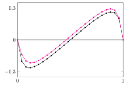
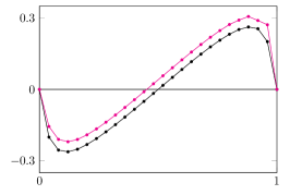
Figure 1: Exact ( ) and approximate ( ) solutions for benchmark 1: centered (left), strong (middle), and weak (right).

3 Time-dependent convection-diffusion equation

We now turn to the time-dependent problem, considering the one-dimensional, $1$-periodic in space, convection-diffusion equation. We seek function $\phi=\phi(x,t)$ solution of

$$\phi_{t}=\mathfrak{E}[\phi]+f,\quad\text{in }\Omega\times(0,t_{\text{f}}],$$ (12)

where $f=f(x,t)$ is a regular, $1$-periodic in space, source term, and $t_{\text{f}}>0$ is the final time. Initial condition is prescribed with $\phi(x,0)=\phi^{0}(x)$, $x\in\Omega$, while the periodic condition reads $\phi(0,t)=\phi(1,t)$, $t>0$.

Applying the method of lines, we seek for an approximation of the solution of the ordinary differential system of equations

$$\frac{\text{d}\Phi}{\text{d}t}=A\Phi+F,\quad\text{in }(0,t_{\text{f}}],$$ (13)

where vector $\Phi=\Phi(t)=(\phi_{i}(t))_{i=1}^{I}$, $\phi_{i}(t)\approx\phi(x_{i},t)$, and $A=A(\theta_{3},\theta_{4},Pe)$ is the circulant matrix associated to the scheme parameterised with $\theta_{3}$, $\theta_{4}$, and $Pe$. On the other hand, $F=F(t)=(f_{i}(t))_{i=1}^{I}$, $f_{i}(t)=f(x_{i},t)$, while the initial condition is given by $\phi_{i}(0)=\phi(x_{i},0)$.

3.1 Time discretisation

We aim at designing a multi-stage Runge-Kutta (RK) method to compute numerical approximations in time that provides the better trade-off between stability, accuracy, and positivity taking into account the cell Péclet number $Pe$ and the parameterisation of the spatial scheme with respect to $\theta_{3}$ and $\theta_{4}$.

Let $N$ be a positive integer and $(t^{n})_{n=0}^{N}$ the discrete times. We consider the uniform subdivision $t^{n}=n\Delta t$, $n=0,\ldots,N$, with the time step $\Delta t=\frac{t_{\text{f}}}{N}$. The generic $s$-stage Runge-Kutta method to solve the initial value ODE system (13) is given by

$$\Phi^{n,j}=\Phi^{n}+\Delta t\sum_{\ell=1}^{s}a_{j\ell}\mathcal{K}^{n,\ell},$$

$$\Phi^{n+1}=\Phi^{n}+\Delta t\sum_{j=1}^{s}b_{j}\mathcal{K}^{n,j},$$

$$\mathcal{K}^{n,j}=A\Phi^{n,j}+F(t^{n,j}),\quad j=1,\ldots,s,$$

where $\Phi^{n}=(\phi_{i}^{n})_{i=1}^{I}$, $\phi_{i}^{n}\approx\phi(x_{i},t^{n})$, and $\Phi^{n,j}=(\phi_{i}^{n,j})_{i=1}^{I}$, $\phi_{i}^{n,j}\approx\phi(x_{i},t^{n,j})$, with $t^{n,j}=t^{n}+\Delta tc_{j}$, are the intermediate time sub-steps.

We store the entries $(a_{j\ell})$, $(b_{j})$, and $(c_{j})$ in matrix $A_{\text{BT}}\in\mathbb{R}^{s\times s}$, vectors $b_{\text{BT}}\in\mathbb{R}^{s}$ and $c_{\text{BT}}\in\mathbb{R}^{s}$ respectively, presented in a table called Butcher tableau:

$c_{\text{BT}}$	$A_{\text{BT}}$
	$b_{\text{BT}}$

=

$c_{1}$	$a_{11}$	$\cdots$	$a_{1s}$
$\vdots$	$\vdots$		$\vdots$
$c_{s}$	$a_{s1}$	$\cdots$	$a_{ss}$
	$b_{1}$	$\cdots$	$b_{s}$

.

Notice that the explicit Runge-Kutta is achieved if $a_{ij}=0$ for $i\leq j$.

Equation (13) leads to the uncoupled linear differential system

$$\frac{\text{d}\tilde{\phi}_{i}}{\text{d}t}=\lambda_{i}(\theta_{3},\theta_{4},Pe)\tilde{\phi}_{i}+\tilde{f}_{i},\qquad\tilde{\phi}_{i}(0)=\tilde{\phi}_{i}^{0},\quad i=1,\ldots,I,$$ (14)

taking into account the circulant matrix $A$ eigenvalues given by equation (5), where $\tilde{\phi}_{i}=\tilde{\phi}_{i}(t)$ and $\tilde{f}_{i}=\tilde{f}_{i}(t)$ are the projections of $\phi_{i}$ and $f_{i}$, respectively, on the eigenbasis.

To deal with the stability of the Runge-Kutta scheme, we consider the homogeneous problem deriving from (14), by cancelling the source term $\tilde{f}_{i}$. Let $z_{i}=\Delta t\lambda_{i}(\theta_{3},\theta_{4},Pe)$. The $s$-stage order $p$ explicit Runge-Kutta scheme for the homogeneous equation associated with equation (14) reads

$${\tilde{\phi}}^{n+1}_{i}=R_{ps}(z_{i};w_{p+1},\ldots,w_{s}){\tilde{\phi}}^{n}_{i},\quad\textrm{with}\quad R_{ps}(z;w_{p+1},\ldots,w_{s})=1+\sum_{k=1}^{p}\frac{z^{k}}{k!}+\sum_{k=p+1}^{s}w_{k}z^{k},\quad z\in\mathbb{C},$$ (15)

where $R_{ps}$ is the polynomial transfer function and $w_{k}\in\mathbb{R}$, $k=p+1,\ldots,s$, stand for the free parameters when $p<s$. No free parameters are available if $s=p$ and we just denote $R_{p}(z)\equiv R_{pp}(z;)$ for the sake of simplicity. We recall that stability scheme is achieved when the complex values $z$ are such that the absolute value of polynomial $R_{ps}$ is lower than one and the set

$$\textrm{S\hskip-1.0ptR}_{ps}(w_{p+1},\ldots,w_{s})=\{z\in\mathbb{C}:|R_{ps}(z;w_{p+1},\ldots,w_{s})|<1\},$$ (16)

characterises the absolute stability region [15]. In addition, for $s=p$, we denote $\textrm{S\hskip-1.0ptR}_{p}\equiv\textrm{S\hskip-1.0ptR}_{pp}$.

As an example, we plot in Figure 2 the stability regions for three classical schemes: (i) $\textrm{S\hskip-1.0ptR}_{2}$ — order 2 with $w_{3}=w_{4}=0$, (ii) $\textrm{S\hskip-1.0ptR}_{3}$ — order 3 with $w_{3}=\frac{1}{6}$, $w_{4}=0$, and (iii) $\textrm{S\hskip-1.0ptR}_{4}$ — order 4 with $w_{3}=\frac{1}{6}$, $w_{4}=\frac{1}{24}$.

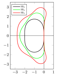
Figure 2: Stability regions of classical Runge-Kutta methods RK₂, RK₃, and RK₄.

3.2 Design of Optimal Absolute stability regions

The goal is to design an efficient explicit Runge-Kutta method allowing step sizes as large as possible, still preserving the linear stability. The key idea of the optimisation of Runge-Kutta methods for temporal integration is to determine the parameters that yield both the largest stability limit and the highest accuracy (expressed in terms of dissipation and dispersion). In [16], the authors focus on constructing a stability polynomial which allows the largest absolutely stable step size and corresponding Runge - Kutta method (number of stages and Butcher tableau) for a given problem when the spectrum of the initial value problem is known. They formulated a stability optimisation problem and constructed an algorithm based on convex optimisation techniques. They considered a global convergence in the case that the order of approximation is one and the spectrum encloses a star-like region. Their optimality criterium is the stability of the method. Ait-Haddou in [3] used the theory of polar forms of polynomials to obtain sharp bounds on the radius of the largest disc (absolute stability radius), and on the length of the largest possible real interval (parabolic stability radius) to be inscribed in the stability region associated to the stability polynomial of an explicit Runge-Kutta method. Schlegel et. al. [22] constructed a multirate time-step integration method for the convection equation. The method decouples different physical regions so that the time step size constraint becomes a local instead of a global restriction. Moreover, Schlegel introduced a generic recursive multirate Runge-Kutta scheme of third order accuracy. In [18], the author developed an optimization of the explicit two-derivative sixth-order Runge–Kutta method in order to obtain low dissipation and dispersion errors. The method depends on two free parameters, used for the optimisation and the spatial derivatives are discretized by finite differences and Petrov–Galerkin approximations.

In this study, we focus on 4-stage RK schemes ($s=4$) at least second-order ($p\geq 2$) as a guideline for a more general situation. As indicated by Table 5, the shape of spectral curve $\mathcal{s}\to\lambda(\mathcal{s};\theta_{3},\theta_{4},Pe)$ highly depends on the cell Péclet number and the parameters values. On the other hand, stability regions are controlled by $w_{3}$ and $w_{4}$ parameters and should be adapted in function of the spectrum curve to optimally embedded the curve into $\textrm{S\hskip-1.0ptR}_{ps}(w_{3},w_{4})$. Such an optimisation problem is almost intractable due to the high non-linearity involved in the construction of the functional to minimise and we observe there exist three major scenarios: (A) the spectral curve is almost vertical, (B) almost horizontal, and (C) an intermediate case (see Table 5). Consequently, we aim to determine two absolute stability regions corresponding to the two extreme scenarios.

3.2.1 The imaginary axis

Scenario (A) takes place for low diffusion schemes where the spectral curve is getting closer to the vertical axis as long as the Péclet number increases. We also deal with the fourth-order centered scheme where the spectrum lies “near” the left of the imaginary axis. Consequently, one has to design a RK scheme by seeking real constants $w_{3}$ and $w_{4}$ such that the stability region includes the largest segment of the imaginary axis centred at the origin.

The solution is given by the following optimisation problem

$$\max_{w_{3},w_{4}\in\mathbb{R}}\,\Big{\{}\eta;\ [-\eta\mathfrak{i},\eta\mathfrak{i}]\subset\textrm{S\hskip-1.0ptR}_{24}(w_{3},w_{4})\Big{\}},$$

but no analytical solution can be exhibited. Nevertheless, in [15], the authors present a solution of the optimal problem when one maximises $\eta$ for the three-parameters functional $\textrm{S\hskip-1.0ptR}_{14}(w_{2},w_{3},w_{4})$ (which contains the particular case $\textrm{S\hskip-1.0ptR}_{24}(w_{3},w_{4})$, since we have one more free parameter). It is shown that polynomial

$$P_{4}(z)=1+z+\frac{5}{9}z^{2}+\frac{4}{27}z^{3}+\frac{4}{81}z^{4}$$

provides the best largest segment of the imaginary axis with $\eta_{\max}=3$.

We plot in Figure 3 the two stability regions associated to the popular RK₄ scheme and the optimal solution proposed in [15]. We observe that the RK₄ scheme provides an excellent approximation with $\eta_{\max}=2\sqrt{2}$, [15]. Of course, the optimal case would provide a slightly bigger $\eta_{\max}$, but we consider that, for our application, the RK₄ is an excellent candidate for the first scenario.

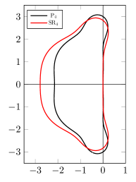
Figure 3: Stability region associated to polynomials $P_{4}$ and R₄.

3.2.2 The real axis

Scenario (B) concerns numerical schemes with large diffusion characterised by low Péclet numbers. Therefore, we seek real constants $w_{3}$ and $w_{4}$ such that the stability region includes the largest segment of the negative real axis starting at the origin. An additional difficulty is that the stability region may not be a simply connected region as exemplified in Figure 4. Consequently, we only consider the first connected region which contains the origin as the effective stability region. There are also stabilized explicit Runge - Kutta methods as, for example, Runge - Kutta - Chebyshev methods (RKC) dedicated to extended real stability intervals and useful for semi-discrete parabolic problems. A second-order RKC method was initially proposed by van der Houwen and Sommeijer [14] and a family of second- and fourth- order Orthogonal - Runge - Kutta - Chebyshev methods (ROCK) were proposed by Abdulle and Abdulle and Medovikov, [1, 2] but as we said these methods are based on Runge - Kutta and for our purposes, we only deal with original Runge - kutta.

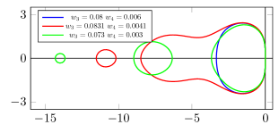
Figure 4: Stability regions for different values of $w_{3}$ and $w_{4}$.

Riha, in [21], proved that the optimal stability polynomial $\bar{R}_{ps}(z)$ of order $p$ and degree $s$

$$\bar{R}_{ps}(z;\bar{w}_{1},\ldots,\bar{w}_{s})=1+\sum_{k=1}^{p}\frac{z^{k}}{k!}+\sum_{k=p+1}^{s}\bar{w}_{k}z^{k}$$

such that

$$|\bar{R}_{ps}(z;\bar{w}_{1},\ldots,\bar{w}_{s})|\leq 1,\quad z\in[-\zeta,0],$$

is unique and satisfies the so-called ripple property:

Property 1 (ripple property)

Polynomial $R_{ps}(z;w_{1},\ldots,w_{s})$ satisfies the ripple property, if and only if, there exist $s-p+1$ points $x_{0}<x_{1}<\ldots<x_{s-p}<0$, with $x_{0}=-\zeta_{\max}$, such that

$$R_{ps}(x_{i};w_{1},\ldots,w_{s}) =-R_{ps}(x_{i+1};w_{1},\ldots,w_{s}), \quad i=0,1,\ldots,s-p-1,$$

$$|R_{ps}(x_{i};w_{1},\ldots,w_{s})| =1, \quad i=0,1,\ldots,s-p.$$

There are no explicit analytic expressions for the optimal $s-p+1$ coefficients $w_{k}$, $k=p+1,\ldots,s$, but the ripple property has been used to construct approximations to the optimal stability polynomial $R_{ps}(z)$ as proposed for example in [15, 23], where the authors show that the optimal bound $\zeta_{\max}$ depends on $s$ and satisfies $\zeta_{\max}=c_{p}s^{2}$, $c_{p}\in\mathbb{R}$, asymptotically with $s\to\infty$.

For $p=2$, there is a suitable approximate polynomial $B_{s}$ based on Chebyshev polynomials, given by M. Bakker in 1971, that generates about $80\%$ of the optimal interval and for $s=4$, the Bakker polynomial reads

$$B_{4}(z)=1+z+\frac{z^{2}}{2}+\frac{2z^{3}}{25}+\frac{z^{4}}{250},$$ (17)

where $\zeta_{\max}=10$, $w_{3}=\frac{2}{25}$, and $w_{4}=\frac{1}{250}$. We plot in Figure 5 the Baker polynomial representation and the corresponding stability region.

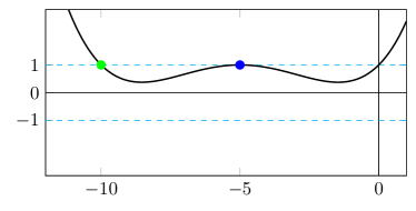
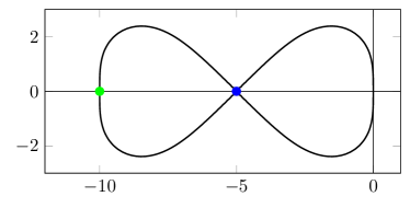
Figure 5: Baker polynomial $B_{4}=R_{24}(x;\frac{2}{25},\frac{1}{250})$ graph (left) and the corresponding stability region (right).

Such a stability region is suitable for $Pe=0$ but not for small values of $Pe$ since it is not radial at the origin. Consequently, we have considered a small perturbation of parameters $w_{3}$ and $w_{4}$ in order to produce a radial region still preserving a large interval on the real negative axis. We found a good trade-off with $w_{3}=0.0834$ and $w_{4}=0.0042$ providing $\zeta_{\max}\approx 11$. We plot in Figure 6 the polynomial curve and the corresponding region.

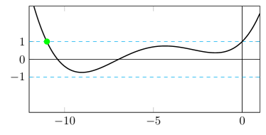
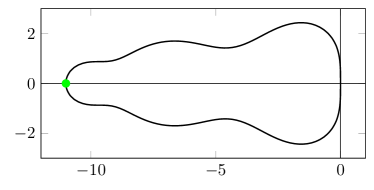
Figure 6: Polynomial $R_{24}\mathopen{}\mathclose{{}\left(x;0.083,0.0042}\right)$ graph (left) and the corresponding stability region (right).

3.2.3 Design of a non-negative scheme

A critical issue in some problems is to guarantee the positivity of the solution. Indeed, temperature, concentration, or density are physical quantities that must be non negative at the discrete level. Figure 6 shows that the polynomial does not satisfy this criterion. For instance, if $x\in]-10.3997,-6.9570[$, the scheme is stable but the polynomial is negative leading to a sign change.

We then consider a more constrained problem and define the new optimisation problem

$$\max_{w_{3},w_{4}\in\mathbb{R}}\Big{\{}\zeta;0.01\leq R_{24}(x;w_{3},w_{4})\leq 0.7,\forall x\in[-\zeta,0]\Big{\}},$$

to create the appropriated region. The lower bound $0.01$ and upper bound $0.7$ are prescribed in order to provide a radial domain. Indeed, extreme bound values $0.0$ and $1.0$ provide a stability region similar to Bakker polynomial displayed in Figure 5.

Numerical solution of the optimal problem provides $w_{3}=\frac{603}{6998}$ and $w_{4}=\frac{15}{3212}$ with $\zeta_{\max}\approx 9.43$ and we plot in Figure 7 the polynomial curve and the corresponding stability region. We obtain a large radial stability region with $\zeta_{\max}$ close to the one provided by the Bakker polynomial. On the other hand, the domain still preserves an important part of the horizontal axis in comparison to the non positive optimal case given in Figure 6.

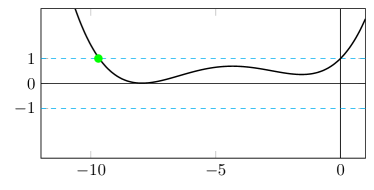
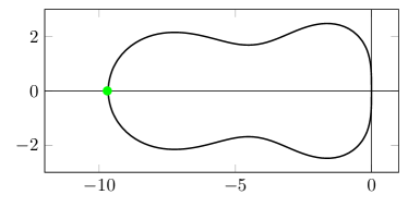
Figure 7: Polynomial $R_{\text{D}}(x)$ graph (left) and the corresponding stability region (right).

To conclude the analysis, scenario (A) concerns the low diffusive situation and the $R_{4}$ polynomial is well adapted for such situation. On the other hand, scenario (B) deals with high diffusive operator and the polynomial

$$R_{\text{D}}(z)=R_{24}\mathopen{}\mathclose{{}\left(z;\frac{603}{6998},\frac{15}{3212}}\right)$$

provides an excellent stability region.

3.3 Butcher tableau construction

Stability issue provides coefficients $w_{3}$ and $w_{4}$ for polynomial $R_{\text{D}}$ and one has to compute corresponding entries of Butcher tableau. We briefly outline the method for the general case $R_{24}(z;w_{3},w_{4})$ and provide the Butcher’s tableau for the two scenarios, taking into account a crucial restriction: the two tableaux must have the same time sub-steps for the sake of compatibility.

An explicit 4-stage Runge-Kutta method is given by the generic Butcher tableau

$c_{1}$	0	0	0	0
$c_{2}$	$a_{21}$	0	0	0
$c_{3}$	$a_{31}$	$a_{32}$	0	0
$c_{4}$	$a_{41}$	$a_{42}$	$a_{43}$	0
	$b_{1}$	$b_{2}$	$b_{3}$	$b_{4}$

Consistency yields

$$c_{i}=\sum_{j=1}^{i-1}a_{ij},\quad i=1,\ldots,4,$$

while the second-order assumption provides the constraints

$$\begin{bmatrix}1&1&1&1\end{bmatrix}b=1,\quad b^{\text{T}}c=\frac{1}{2}.$$ (18)

Additional constraints are considered:

• The Runge-Kutta scheme is fourth-order for the non-homogeneous equation $\phi^{\prime}(t)=f(t)$,

  $$\begin{bmatrix}(c_{1})^{2}&(c_{2})^{2}&(c_{3})^{2}&(c_{4})^{2}\end{bmatrix}b=\frac{1}{3},\qquad\begin{bmatrix}(c_{1})^{3}&(c_{2})^{3}&(c_{3})^{3}&(c_{4})^{3}\end{bmatrix}b=\frac{1}{4}.$$ (19)

• The four stage method has to satisfy the consistency condition to suit the polynomial $R_{24}(z;w_{3},w_{4})$,

  $$b^{\text{T}}Ac=w_{3},\qquad b^{\text{T}}A^{2}c=w_{4}.$$ (20)

Conditions (18), (19), and (20) are equivalent to the system

$$V^{\text{T}}b^{\text{T}}=\begin{bmatrix}1&1&1&1\\ c_{1}&c_{2}&c_{3}&c_{4}\\ c_{1}^{2}&c_{2}^{2}&c_{3}^{2}&c_{4}^{2}\\ c_{1}^{3}&c_{2}^{3}&c_{3}^{3}&c_{4}^{3}\\ \end{bmatrix}\begin{bmatrix}b_{1}\\ b_{2}\\ b_{3}\\ b_{4}\\ \end{bmatrix}=\begin{bmatrix}1\\ 1/2\\ 1/3\\ 1/4\\ \end{bmatrix}$$ (21)

together with equations

$$b_{3}a_{32}c_{2}+b_{4}(a_{42}c_{2}+a_{43}c_{3})=w_{3}$$ (22)

$$b_{4}a_{43}a_{32}c_{2}=w_{4}.$$ (23)

Assuming $c_{1}=0$, the determinant of the Vandermonde matrix $V$ is $(c_{4}-c_{3})(c_{3}-c_{2})c_{2}$ and two situations arise:

• If $c_{2}\neq 0$, $c_{4}\neq c_{3}$, and $c_{3}\neq c_{2}$, the system has a unique solution $b$. Hence in this case, we choose the free parameters to be $c_{2}$, $c_{3}$, $c_{4}$, and $a_{43}$. From the Vandermonde system, we obtain $b$.

• If $c_{2}=0$ or $c_{4}=c_{3}$ or $c_{3}=c_{2}$, we have a dependent linear system. For instance, assuming that $c_{2}=c_{3}$, system (21) turns to be

  $$\begin{bmatrix}1&1&1&1\\ 0&c_{2}&c_{2}&c_{4}\\ 0&0&0&c_{4}(c_{4}-c_{2})\\ 0&0&0&0\\ \end{bmatrix}\begin{bmatrix}b_{1}\\ b_{2}\\ b_{3}\\ b_{4}\\ \end{bmatrix}=\begin{bmatrix}1\\ 1/2\\ 1/3-c_{2}/2\\ 1/4-(c_{4}+c_{2})/3+c_{4}c_{2}/2\\ \end{bmatrix}.$$ (24)

  The system has several degrees of freedom we have to fix with relations

  $$\frac{1}{4}-\frac{c_{4}+c_{2}}{3}+\frac{c_{4}c_{2}}{2}=0,\quad c_{4}(c_{4}-c_{2})\neq 0,\quad c_{2}\neq 0.$$

  We get vector $b$ with

  $$b_{4}=\frac{2-3c_{2}}{6c_{4}(c_{4}-c_{2})},\quad b_{3}=\frac{3c_{4}-2}{6c_{2}(c_{4}-c_{2})}-b_{2},\quad b_{1}=\frac{c_{4}+c_{2}-1}{6c_{2}c_{4}}.$$

  Notice that the user has to choose the free parameters $c_{2}$, $a_{43}$, and $b_{2}$.

From vectors $c$ and $b$, we compute the remaining Butcher tableau elements $a_{21}$, $a_{31}$, $a_{32}$, $a_{41}$, and $a_{42}$ and we obtain

$$a_{21}=c_{2},\,\,\,a_{32}=\frac{w_{4}}{b_{4}a_{43}c_{2}},\,\,\,a_{42}=\frac{w_{3}-b_{4}a_{43}c_{3}-b_{3}c_{2}a_{32}}{b_{4}c_{2}},\,\,\,a_{31}=c_{3}-a_{32},\,\,\,a_{41}=c_{4}-a_{42}-a_{43}.$$

At last, we present in Table 6 the two Butcher tableaux with 4-stage corresponding to $R_{4}$ and $R_{\text{D}}$ polynomials. We tag the associated methods as RK₄ and RK${}_{\text{D}}$, respectively. It is important to notice that the RK${}_{\text{D}}$ has been designed with the same time sub-steps according to the classical RK₄ scheme.

Table 6: Butcher tableaux for the classical scheme $\text{RK}_{4}$ (left) and RK${}_{\text{D}}$ (right).

0	0	0	0	0
1/2	1/2	0	0	0
1/2	0	1/2	0	0
1	0	0	1	0
	1/6	1/3	1/3	1/6

0	0	0	0	0
1/2	1/2	0	0	0
1/2	334/861	373/3328	0	0
1	481/3310	587/1655	1/2	0
	1/6	0.4	4/15	1/6

4 Optimal time step for stability

We now reach the key point of the paper: the confrontation between the RK stability region with the spatial operator spectrum. More precisely, we have, on the one hand, a complex value parametric curve given by relation (6), $\mathcal{s}\in[0,1]\to\lambda(\mathcal{s};\theta_{3},\theta_{4},Pe)$ that contains all the eigenvalues $\lambda_{i}$ of the discrete operator. On the other hand, applying the RK scheme with time step $\Delta t$ and setting $z_{i}=\Delta t\lambda_{i}(\theta_{3},\theta_{4},Pe)$, one has to choose $\Delta t$ small enough such that $z_{i}\in\textrm{S\hskip-1.0ptR}_{ps}(w_{p+1},\ldots,w_{s})$ to guarantee the stability.

4.1 The CFL condition

Let

$$z(\mathcal{s};\theta_{3},\theta_{4},Pe)=\Delta t\lambda(\mathcal{s};\theta_{3},\theta_{4},Pe)=C_{\text{CFL}}\,\rho(\mathcal{s};\theta_{3},\theta_{4},Pe),$$ (25)

where $C_{\text{CFL}}=\frac{u\Delta t}{\Delta x}$ and $\rho$ be given by relation (7) for $u\neq 0$. Stability condition for the discrete problem is achieved if we satisfy the condition

$$C_{\text{CFL}}\,\rho(\mathcal{s};\theta_{3},\theta_{4},Pe)\subset\textrm{S\hskip-1.0ptR}_{24}(w_{3},w_{4}),\quad\mathcal{s}\in[0,1].$$ (26)

Note that the scheme stability depend on the six parameters $\theta_{3}$, $\theta_{4}$, $w_{3}$, $w_{4}$, $Pe$, and $C_{\text{CFL}}$ and the goal of this section is to analyse the stability of the full time-dependent convection-diffusion equation.

Remark 3

The stability condition combines two main ingredients. On the one hand, the shape of the stability region is characterised by function $\rho$ that provides a complex value curve where all the eigenvalues lie, independently of the space parameter $\Delta x$. On the other hand, the CFL value $C_{\text{CFL}}$ scales the previous curve to fit inside the stability region.

Assuming that scheme in space is given (parameters $\theta_{3}$, $\theta_{4}$ are prescribed) and the scheme in time is given (parameters $w_{3}$, $w_{4}$ are prescribed), we define the optimal CFL curve as a function of the Péclet number

$$Pe\to\widehat{C}_{\text{CFL}}(Pe)=\lim\sup\Big{\{}C_{\text{CFL}}\geq 0,\text{ such that }\eqref{eq:stability_CFL}\text{ holds}\Big{\}}.$$

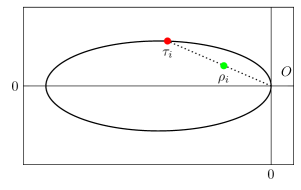
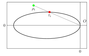
Figure 8: How to calculate the limiting scaling factor: $\widehat{C}_{\text{CFL}}>1$ (left) and $\widehat{C}_{\text{CFL}}<1$ (right).

We compute $\widehat{C}_{\text{CFL}}(Pe)=\widehat{C}_{\text{CFL}}(Pe;\theta_{3},\theta_{4},w_{3},w_{4})$ with the following algorithm (see Figure 8):

• Compute eigenvalues $\rho_{i}$, $i=1,\ldots,I$, from the space discretisation operator spectrum;

• Compute intersection points $\tau_{i}$ of the segment line $O\rho_{i}$ with the stability region boundary;

• Compute $\displaystyle\widehat{C}_{\text{CFL}}=\min_{i=1,\ldots,I}\frac{|\tau_{i}|}{|\rho_{i}|}$.

Afterwards the maximum stable time step is given by

$$\Delta t_{\max}=\frac{\widehat{C}_{\text{CFL}}\Delta x}{u}.$$ (27)

Remark 4

Two extreme situations require a specific treatment.

• If $Pe=0$, i.e., $u=0$, a CFL constant based on the velocity is no longer available. In that case, the spectrum is given in Table 1 for the centered scheme, Table 2 for the weak upwind, Table 3 for the strong upwind and reads

  $$\Delta t\lambda(\mathcal{s})=C_{\text{CFL}}\,\rho(\mathcal{s})=\frac{\kappa\Delta t}{\Delta x^{2}}\,2(\cos(2\pi\mathcal{s})-1)\mathopen{}\mathclose{{}\left\{\begin{array}[]{ll}(\frac{7}{6}-\frac{1}{6}\cos(2\pi\mathcal{s}))&\textrm{centered},\\ 1&\textrm{weak},\\ (\cos(2\pi\mathcal{s})-\mathfrak{i}\sin(2\pi\mathcal{s}))&\textrm{strong}.\end{array}}\right.$$

  In this case the maximum stable time step is given by

  $$\Delta t_{\max}=\frac{\widehat{C}_{\text{CFL}}\Delta x^{2}}{\kappa}.$$

• If $Pe=+\infty$, i.e., $\kappa=0$, one has to pass to the limit to determine the spectrum curve, remaining (27) valid.

As an example, we present in Figure 9 two situations with $Pe=5$ and $Pe=10$ where we adjust the CFL constant to fit the spectrum into the stability region: centered scheme in space with the RK₄ scheme in time (top left) and the RK_D (down left) while the pictures in second column present the weak upwind case.

	centered	weak upwind
	$Pe=10$, $\widehat{C}_{\text{CFL}}=2.0935$, $\Delta t_{\max}=0.0837$	$Pe=5$, $\widehat{C}_{\text{CFL}}=1.3117$, $\Delta t_{\max}=0.0525$
RK4
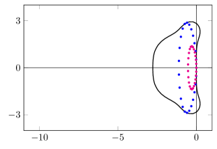
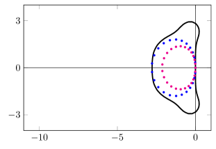
	$Pe=10$, $\widehat{C}_{\text{CFL}}=1.3479$, $\Delta t_{\max}=0.0539$	$Pe=5$, $\widehat{C}_{\text{CFL}}=1.7948$, $\Delta t_{\max}=0.0718$
RK${}_{\text{D}}$

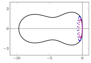
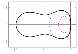
Figure 9: Examples of stability regions (    boundary of stability region;    “discrete” $\rho$;    “discrete” $\widehat{C}_{\text{CFL}}\,\rho$).

4.1.1 Analysis of spatial schemes

A full discretised scheme consists in fixing the time and spatial scheme parameters. We have identified two schemes in time — RK${}_{\text{D}}$ and RK₄ — for low and high Péclet situations and three schemes in space — centered, weak upwind, and strong upwind. We shall discard the strong upwind scheme due to the high dispersion effect. Indeed, let us consider the advection problem $\mathfrak{E}[\phi]=0$ with $u=1$ and $\kappa=0$ ($Pe=+\infty$). Function

$$\phi(x,t;\omega)=\sin(2\pi\omega(x-ut))$$

with $\omega=3$, is a periodic solution. We carry out the numerical simulation with the RK₄ scheme in time and the three schemes in space with $\Delta t=\Delta t_{\max}$ (see expression (27)) until the final time $t_{\text{f}}=1$. We plot the numerical solutions in Figure 10 computed with $I=25$ and $I=50$ nodes — benchmark 2. We observe the large phase errors produced by the strong upwind scheme which justify the choice to discard it.

$I$	centered	weak upwind	strong upwind
25
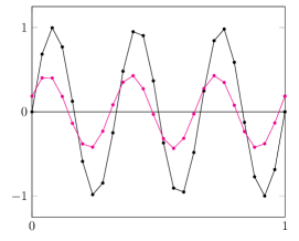
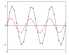
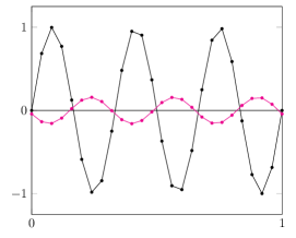
50

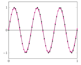
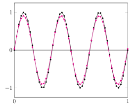
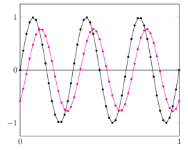
Figure 10: Exact ( ) and approximate ( ) solutions considering RK₄ time scheme for benchmark 2.

We turn to a situation where a rough function is convected ($u=1$, $\kappa=0$, $Pe=+\infty$) and compare the centered and weak upwind scheme. The manufactured solution is given by

$$\phi(x,t;\delta)=\frac{1}{\pi}\mathopen{}\mathclose{{}\left(1-\frac{2}{\pi}\arccos((1-\delta)\sin(\pi(x-t-\frac{1}{2})))}\right)\mathopen{}\mathclose{{}\left(\arctan(\frac{1}{\delta}\sin(\pi(x-t)))}\right)$$ (28)

with $\delta=0.01$ that corresponds to a rough solution due to the sharp transition. The numerical solutions are computed with the RK${}_{\text{4}}$ scheme in time taking $\Delta t=\Delta t_{\max}$, $I=25$, and the centered and weak upwind schemes in space — benchmark 3.

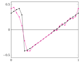
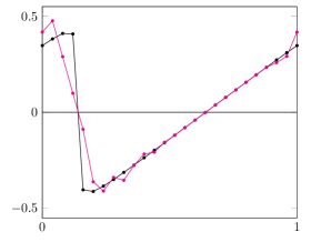
Figure 11: Exact ( ) and approximate ( ) solutions for $t_{\text{f}}=2\Delta t_{\max}$ considering RK₄ time scheme for benchmark 3: centered (left) and weak upwind (right).

In Figure 11 we present the numerical solutions after two time steps. We observe the centered scheme is more unstable with a larger number of over- and undershoots. Of course, a definitive method would consist in employing a high viscous scheme (the simple two-points upwind one) but with a dramatic cut of the accuracy. Hence, the weak upwind scheme is regarded as an alternative to the centered one when large oscillations appear.

4.1.2 Optimal CFL curves

The curves $Pe\to\widehat{C}_{\text{CFL}}(Pe;\theta_{3},\theta_{4},w_{3},w_{4})$ are determined for the four situations we want to highlight: RK₄ and RK${}_{\text{D}}$ for time; centered and weak upwind for space. We plot in Figure 12 the optimal CFL curves for the fourth-order centered scheme and the third order weak upwind scheme with $Pe\in[0.001,20]$ (note that the oscillations we observe for the centered case are a consequence of the discrete consideration of the spectral curve). We complement the figure with Table 7 indicating the optimal CFL values, $\widehat{C}_{\text{CFL}}$, for $Pe=0$ (an expression depending on $\Delta x$) and large Péclet values.

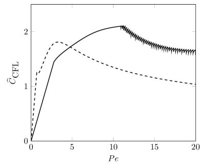
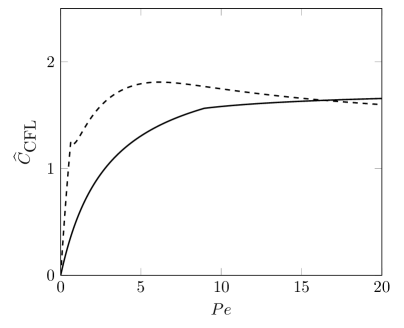
Figure 12: $Pe\to\widehat{C}_{\text{CFL}}$ curves for the four scenarios that we are considering: centered (left) and weak upwind (right), with solid — RK₄, dashed — RK${}_{\text{D}}$.

Table 7: Comparison of $\widehat{C}_{\text{CFL}}$ for RK${}_{\text{D}}$ and RK₄.

$Pe$	RK${}_{\text{D}}$		RK4
	centered	weak upwind	centered	weak upwind
0	$1.77\Delta x^{2}$	$2.36\Delta x^{2}$	$0.53\Delta x^{2}$	$0.70\Delta x^{2}$
20	1.04	1.60	1.62	1.66
200	0.45	1.34	2.04	1.74
20000	0.09	1.25	2.06	1.75
200000	0.04	1.24	2.06	1.75
$+\infty$	0	1.24	2.55	1.75

From Figure 12 and Table 7 we draw the following conclusions:

• centered scheme RK${}_{\text{D}}$ provides the largest time-steps for $Pe<5$ while RK₄ is more efficient for $Pe>5$. In particular, the limit for $Pe\to+\infty$ of $\widehat{C}_{\text{CFL}}$ is 2.55 for RK₄ while $\widehat{C}_{\text{CFL}}$ converges to 0 with RK${}_{\text{D}}$.

• weak upwind scheme For $Pe<15$, $\widehat{C}_{\text{CFL}}$ value is larger with RK${}_{\text{D}}$ scheme than RK₄. The particular case $Pe=0$ shows that RK${}_{\text{D}}$ case allows a time parameter about three times larger than the RK₄ case. For $Pe>15$, RK₄ method turns out to be more efficient.

4.1.3 Convergence order and stability

To compare the convergence error between the centered and the weak upwind discretisations, we consider the advection ($u=1$, $\kappa=0$, $Pe=+\infty$) of the manufactured solution (28) with $\delta=0.1$, corresponding to a smooth solution since the transition takes place in more than 5 nodes. — benchmark 4. We carry out the RK₄ scheme in time with a time step $\Delta t=0.8\Delta t_{\max}$ until $t_{\text{f}}=1$. We present in Table 8 the time step, error $E_{\infty}$

$$E_{\infty}\equiv E_{\infty}(\Phi^{N},I)=\displaystyle\max_{i=1}^{I}|\phi_{i}^{N}-\phi(x_{i},t_{\text{f}})|,$$

and the respective convergence order $O_{\infty}$ between two solutions/grids $(\Phi_{k},I_{k})$, for $k=1,2$ where $I_{1}<I_{2}$ as

$$O_{\infty}\equiv O_{\infty}\mathopen{}\mathclose{{}\left((\Phi_{1}^{N},I_{1}),(\Phi_{2}^{N},I_{2})}\right)=\frac{|\log E_{\infty}(\Phi_{1}^{N},I_{1})/E_{\infty}(\Phi_{2}^{N},I_{2})|}{|\log I_{1}/I_{2}|},$$

while we display in Figure 13 the numerical approximations for the centered and weak upwind schemes. We reach the fourth-order in space for the centered method and the expected third-order in space for the upwind case (the fourth-order method in time turns to be insignificant for large values of $I$, since small values of $\Delta t$ are needed due to the CFL condition).

Table 8: Time steps and errors using 80% of the maximal time step given by $\widehat{C}_{\text{CFL}}$ considering RK₄ time scheme for benchmark 4.

$I$	centered			weak upwind
	$\Delta t$	$E_{\infty}$	$O_{\infty}$	$\Delta t$	$E_{\infty}$	$O_{\infty}$
100	1.65E$-$2	1.68E$-$2	—	1.40E$-$2	2.20E$-$2	—
200	8.25E$-$3	3.88E$-$3	2.1	6.98E$-$3	6.29E$-$3	1.8
400	4.12E$-$3	4.88E$-$4	3.0	3.49E$-$3	1.20E$-$3	2.4
800	2.06E$-$3	3.83E$-$5	3.7	1.75E$-$3	1.70E$-$4	2.8
1600	1.03E$-$3	2.46E$-$6	4.4	8.73E$-$4	2.15E$-$5	3.0

$I$	centered	weak upwind
25
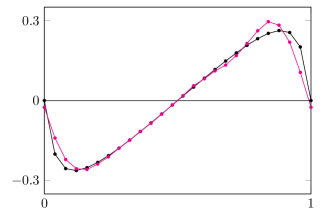
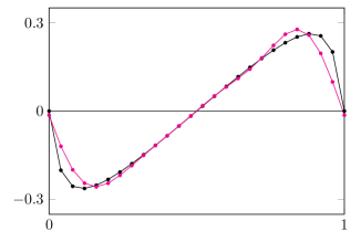
50
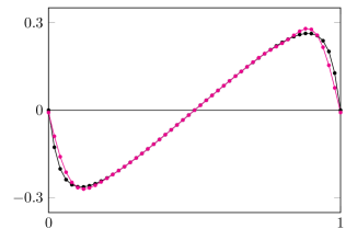
100

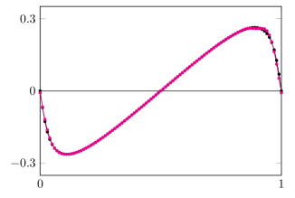
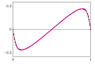
Figure 13: Exact ( ) and approximate ( ) solutions considering RK₄ time scheme for benchmark 4.

To check the stability condition, we have performed the computation with the RK₄ time scheme with three different time steps: (1) the time step $\Delta t_{\max}$ corresponding to the optimal CFL value given by $\widehat{C}_{\text{CFL}}(Pe)$, (2) a $20\%$ smaller time step, and (3) a $10\%$ larger time step. We present in Table 9 the errors $E_{\infty}$ together with the number of iterations $n_{\text{TS}}$ needed to reach the final time $t_{\text{f}}=1$. For the latter case, stability is no longer preserved and the error blows up. With the critical time step $\Delta t_{\max}$, we manage to compute the solution until the final time but with an error slightly larger than the one obtained with the smaller $\Delta t$. Notice that, as expected, the number of steps linearly increases with the number of nodes.

Table 9: Stability study considering RK${}_{\text{4}}$ time scheme for benchmark 4.

$I$	space scheme	$\widehat{C}_{\text{CFL}}$	$\Delta t_{\max}$	$\Delta t=\Delta t_{\max}$		$\Delta t=0.8\Delta t_{\max}$		$\Delta t=1.1\Delta t_{\max}$
				$E_{\infty}$	$n_{\text{TS}}$	$E_{\infty}$	$n_{\text{TS}}$	$E_{\infty}$	$n_{\text{TS}}$
25	centered	2.06	8.25E$-$2	1.13E$-$1	13	9.52E$-$2	16	1.01E$+$1	12
	weak upwind	1.77	7.06E$-$2	1.12E$-$1	15	1.02E$-$1	18	4.62E$-$1	13
50	centered	2.06	4.13E$-$2	5.44E$-$2	25	4.86E$-$2	31	2.35E$+$3	23
	weak upwind	1.75	3.49E$-$2	5.46E$-$2	29	5.05E$-$2	36	4.02E$+$0	27
100	centered	2.06	2.06E$-$2	2.23E$-$2	49	1.68E$-$2	61	1.44E$+$8	45
	weak upwind	1.75	1.75E$-$2	2.45E$-$2	58	2.20E$-$2	72	4.79E$+$2	53
200	centered	2.06	1.03E$-$2	5.87E$-$3	98	3.88E$-$3	122	NaN	89
	weak upwind	1.75	8.73E$-$3	7.05E$-$3	115	6.29E$-$3	144	1.03E$+$7	105

4.2 Hybrid scheme

Hybrid time scheme consists in choosing between the RK₄ and the RK${}_{\text{D}}$ scheme in function of the Péclet number to provide the largest time step. For space (and time) dependent velocity and diffusion coefficient, the scheme then would be different from one node to another. For example, for the centered scheme in space, the left panel of Figure 12 shows that the highest $\widehat{C}_{CFL}(Pe)$ values are reached with the RK${}_{\text{D}}$ scheme when $Pe<5$ while the $\widehat{C}_{CFL}(Pe)$ is larger with RK₄ when $Pe>5$. We implement an hybrid scheme that switches from one method to the other in function of the velocity and diffusion coefficients to optimise the time step and reduce the computational effort.

We consider the space-dependent parameter equation $\partial_{t}\phi+\mathfrak{E}(x)[\phi]=f(x)$ with

$$\mathfrak{E}(x)[\phi]=-u(x)\phi^{\prime}+\kappa(x)\phi^{\prime\prime}$$ (29)

and $f$ a given source term. Since the cell Péclet number depends on the position, we set $\displaystyle Pe_{i}=\frac{u_{i}\Delta x}{\kappa_{i}}$ for node $i$ with $u_{i}=u(x_{i})$ and $\kappa_{i}=\kappa(x_{i})$ for the velocity and diffusion, respectively. Taking the centered scheme for the discretization in space of operator (29), the hybrid scheme in time is obtained with the following rule:

• if $Pe_{i}<5$, we use the RK${}_{\text{D}}$ scheme for node $i$;

• otherwise, we use the RK₄ scheme.

Note that the two time schemes are compatible since we have the same sub-steps by construction.

The weak upwind scheme in space is also considered and the hybrid time scheme derives from the right panel of Figure 12, and is given by:

• if $Pe_{i}<15$, we use the RK${}_{\text{D}}$ scheme for node $i$;

• otherwise, we use the RK₄ scheme.

To update the solution from $t^{n}$ to $t^{n+1}=t^{n}+\Delta t$, we compute the global time step $\Delta t$ in the following way: the Péclet number $Pe_{i}$ and the corresponding optimal CFL number $(\widehat{C}_{CFL})_{i}$ are computed leading to an optimal time step $\Delta t_{i}$ that provides the stability. In order to guarantee the global stability, we then choose

$$\Delta t=\min_{i=1,\ldots,I}\Delta t_{i}.$$ (30)

To test the hybrid scheme, we consider the manufactured solution $\phi(x,t;\omega)=\sin(2\pi\omega(x-ut))$, with $\omega=1$ where the velocity $u=1$ is constant and the diffusion is given by

$$\kappa(x)=a_{0}\exp(25(x-1/2)^{2})+a_{1},\quad a_{0}=10^{-4},\quad a_{1}=10^{-5},$$

— benchmark 5. The source term is calculated to satisfy relation $\partial_{t}\phi=\mathfrak{E}(x)[\phi]+f(x)$ from the manufactured solution. Numerical simulations are carried out until the final time $t_{\text{f}}=1$ with $I=100$. It is worth noting that at the same time step or sub-step, we handle two different schemes in time depending on the cell Péclet number, with different Butcher’s tableaux.

Table 10: Error and number of iterations for the full RK₄ and hybrid scheme for benchmark 5.

scheme	centered			weak upwind
	$\Delta t$	$E_{\infty}$	$n_{\text{TS}}$	$\Delta t$	$E_{\infty}$	$n_{\text{TS}}$
hybrid (RK${}_{\text{4}}$/RK${}_{\text{D}}$)	3.50E$-$3	5.56E$-$5	286	4.38E$-$3	1.46E$-$4	229
RK${}_{\text{4}}$	1.01E$-$3	3.03E$-$6	993	1.26E$-$3	7.80E$-$5	792

We compare the hybrid scheme with the full RK₄ time scheme (which does not depend on the Péclet number) and report in Table 10 the comparison between the two methods. On the one hand, the full RK₄ scheme achieves the better accuracy (errors cut almost by twenty for the centered case and almost by two for the weak upwind) but the hybrid scheme provides the largest time steps with a strong reduction of the number of iterations (almost four times faster). We highlight that no oscillations appear and stability is achieved for both schemes as shown by the errors convergence rate.

We display in Figure 14 the $\widehat{C}_{\text{CFL},\text{RK}_{4}}$ calculated with the full RK₄ scheme and the $\widehat{C}_{\text{CFL},\text{RK}_{\text{D}}}$ with the RK${}_{\text{D}}$ scheme while we highlight the $\widehat{C}_{\text{CFL},\text{hybrid}}$ for the hybrid scheme with the green mark. We observe that, except for a small number of nodes, we have the property

$$\widehat{C}_{\text{CFL},\text{hybrid}}=\max\Big{(}\widehat{C}_{\text{CFL},\text{RK}_{4}},\widehat{C}_{\text{CFL},\text{RK}_{\text{D}}}\Big{)}$$

that confirms we have taken the best scheme in time for each node providing the larger global time step $\Delta t$.

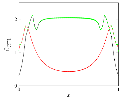
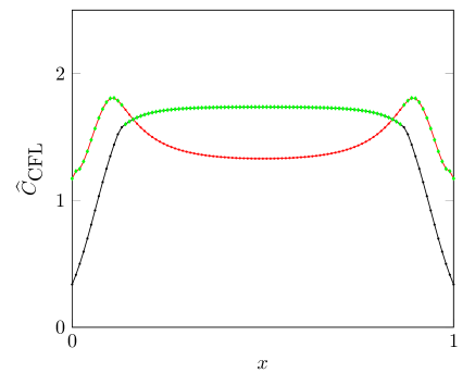
Figure 14: $\widehat{C}_{CFL}$ plots for benchmark 5: centered (left) and weak upwind (right). $\widehat{C}_{\text{CFL},\text{hybrid}}$ values ( ); $\widehat{C}_{\text{CFL},\text{RK}_{4}}$ curve (  ), and $\widehat{C}_{\text{CFL},\text{RK}_{\text{D}}}$ curve ( ).

5 The a posteriori method for optimal time step scheme

At the numerical level, smooth solutions are functions where the numerical derivative is bounded for $\Delta x$ small enough and transitions between successive extremes are spread on, at least, five or six nodes. In that case, even with a large Péclet number, the centered scheme is stable and the time step is ruled by the hybrid scheme condition. On the other hand, to handle sharp gradients or even discontinuities, the weak upwind scheme turns out to be the candidate method substituting the centered scheme, possibly leading to a change of the scheme in time. At time $t^{n}$ and for each node $i$, the scheme in space has to be chosen with respect to the local regularity for that particular node. Then the scheme in time is chosen with respect to the scheme in space, the local cell Péclet, and $\widehat{C}_{CFL}$ to provide the optimal local time step $\Delta t^{n}_{i}$. Then, using the time parameter $\Delta t^{n}$ given by relation (30), we update the solution at time $t^{n+1}$.

In order to make the optimal choice for the space and time schemes (node by node), we use the a posteriori paradigm also mentioned as MOOD method for Multi-dimensional Optimal Order Detector [9, 10]. In this context, the strategy is based on the choice between a high accurate scheme in space (the centered scheme) and a high stable scheme (the weak upwind scheme) together with the associated optimal time scheme we studied in the hybrid scheme section.

5.1 Basics on a posteriori strategy

We present a brief description of the a posteriori paradigm and introduce the notations we need in this section. Assume that the numerical solution $\Phi^{n}$ is known at time $t^{n}$.

1. We compute a candidate solution $\Phi^{\star}$ for time $t^{n+1}$ using the most accurate schemes in space and time, namely the centered scheme and the RK₄.

2. We check, node by node, the admissibility of the solution using detectors, i.e. small routines that analyse specific aspects of the approximations such as extrema, oscillations, and physical property violations if any.

3. The nodes detected as non-admissible are computed again but with the weak upwind and time schemes using the hybrid scheme procedure.

Remark 5

The method is tagged a posteriori since we analyse a candidate solution $\Phi^{\star}$ after computing a time step. On the contrary, MUSCL and WENO method are said a priori since we perform the limitation strategy based on solution $\Phi^{n}$, [19, 20].

5.1.1 Node space and time scheme tables

In practice, we introduce two tables CSS and CTS for Cell Space Scheme and Cell Time Scheme, respectively, with the following rules.

• We set $\texttt{CSS}[i]=0$ if we use the centered scheme otherwise $\texttt{CSS}[i]=1$ for the weak upwind scheme.

• We set $\texttt{CTS}[i]=0$ if we use the RK₄ scheme otherwise $\texttt{CTS}[i]=1$ for the RK${}_{\text{D}}$ scheme.

Given the numerical solution $\Phi^{\star,0}=\Phi^{n}$ and tables CSS and CTS, we rewrite the RK scheme taking the two tables into account. For each node $i$ the terms $\Phi_{i}^{\star,j}$ and $\mathcal{K}_{i}^{\star,j}$ are computed with

$$\Phi_{i}^{\star,j}=\Phi_{i}^{\star,0}+\Delta t\sum_{\ell=1}^{s}a_{j\ell}(\texttt{CTS}[i])\mathcal{K}_{i}^{\star,\ell},$$

$$\Phi_{i}^{\star}=\Phi_{i}^{\star,0}+\Delta t\sum_{j=1}^{s}b_{j}(\texttt{CTS}[i])\mathcal{K}_{i}^{\star,j},$$

$$\mathcal{K}_{i}^{\star,j}=E_{i}(\texttt{CSS}[i])\Phi^{\star,j}+F(x_{i},t^{\star,j}),\quad j=1,\ldots,s.$$

Expressions $a_{j\ell}(\texttt{CTS}[i])$ and $b_{j}(\texttt{CTS}[i])$ indicate that we use RK₄ scheme if $\texttt{CTS}[i]=0$ or RK${}_{\text{D}}$ scheme if $\texttt{CTS}[i]=1$. On the other hand, the term $E_{i}(\texttt{CSS}[i])$ states that we use the centered scheme for node $i$ if $\texttt{CSS}[i]=0$ or the weak upwind scheme if $\texttt{CSS}[i]=1$.

5.1.2 Detectors

Detectors are small routines to check a specific property of the candidate solution. We assemble the detectors in a chain of operations which basically indicate if a node would be cured (change the scheme in space) or not. We list hereafter the detectors we use in the present document and refer to [11] for a detailed presentation of the most useful detectors.

$\bullet$ ED. The Extrema Detector intends to localise the extrema of the numerical function by checking

$$s_{i}=\text{sign}\Big{(}(\phi_{i}^{\star}-\phi_{i+1}^{\star})(\phi_{i}^{\star}-\phi_{i-1}^{\star})\Big{)}.$$

If $s_{i}>0$ we have an extremum and the detector is activated and returns true otherwise it corresponds to a monotone situation and the detector returns false.

$\bullet$ SCD. The Small Curvature Detector helps to select the very small oscillations that we consider innocuous from the stability point of view. We calculate the variation quantity

$$v_{i}=\max\mathopen{}\mathclose{{}\left(\frac{|\phi_{i}^{\star}-\phi_{i+1}^{\star}|}{\Delta x},\frac{|\phi_{i}^{\star}-\phi_{i-1}^{\star}|}{\Delta x}}\right)$$

and, for a user parameter $\theta>0$, the detector returns true if $v_{i}<\theta\Delta x$ and false otherwise since a small value of $v_{i}$ indicates oscillations with too low magnitude to be considered as an issue.

$\bullet$ LOD. Local Oscillation detection aims to detect variations deriving from oscillations. Indeed, a local oscillation is characterised by a variation of the curvature sign. To this end, we compute the second derivative

$$\chi_{i}=\frac{\phi_{i+1}^{\star}-2\phi_{i}^{\star}+\phi_{i-1}^{\star}}{\Delta x}.$$

Then the detector is deactivated (return false) if $\chi_{i-1}$, $\chi_{i}$, and $\chi_{i+1}$ have the same sign and is activated (return true) if one of the curvatures has a different sign of the two others.

$\bullet$ SD. Smooth Detector consists in assessing the local numerical smoothness to determine if an extremum is physical or if it corresponds to a numerical artefact. To evaluate the smoothness of the solution we use, once again, the curvature and define the minimum and maximum absolute curvature

$$\chi_{i,m}=\min(\chi_{i-1},\chi_{i},\chi_{i+1}),\qquad\chi_{i,M}=\max(\chi_{i-1},\chi_{i},\chi_{i+1}).$$

For a given user parameter $\theta\in[0,1]$, the solution is not smooth (detector activated true) if $\chi_{i,m}<\theta\chi_{i,M}$ since we detect large variation of curvature on the three consecutive points. Otherwise, the detector returns false that indicates the solution is considered smooth enough at the numerical level.

5.1.3 Detector chain and a posteriori cure

The detectors being defined, we assemble it into an ordered chain that enables to decide whether a node would be corrected or not.

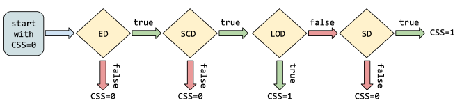
Figure 15: The chain detector.

The detector chain is carried out for nodes with CSS[i]=0, that is the centered scheme. We preserve the high accuracy scheme if there is no extremum (ED false) or generated by too small variations (SCD false). When a potential oscillation is detected (ED true), we try to relax the scheme (and preserve the accuracy) with other detectors that assess if the extremum is a real physical one. The LOD is activated if we observe the sign change of the curvature and then we set $\texttt{CSS}[i]=1$ to indicate that the node has to be cured. In the same way, a node with too large variations of the curvature is considered as a problematic node and we set $\texttt{CSS}[i]=1$ if SD is true. At the end of the chain, we have a new CSS map that indicates the points we have to compute again with the weak upwind scheme. The time scheme is determined with the hybrid scheme strategy and we flag the $\texttt{CTS}[i]$ accordingly.

From the CSS map and the cell Péclet number, we modified the CTS map following the rule given by the hybrid scheme. At the end of the day, we get a new $\Delta t^{n}_{i}$ for each node $i$ and use the minimum time step for $\Delta t^{n}$ following (30).

Remark 6

Computational resources are reduced by only computing again the node $i$ that have been cured together with the neighbour nodes that may be affected by the values of $\Phi_{i}^{\star}$ during the four-stage Runge-Kutta procedure. In practice, very few nodes are modified by the a posteriori correction (less than 5%, see [10]) and the additional cost is of the same order.

5.2 Numerical tests

We present two numerical tests to examine the efficiency of the a posteriori method. The first sanity check consists in carrying out a simulation with a regular solution. Indeed, for smooth approximations, the limiter strategy has to preserve the higher accuracy and the chain detector has to return $\texttt{CSS}[i]=0$ for all nodes $i$. — benchmark 6. We consider the manufactured solution (11) with $\delta=0.15$. We take constant physical parameters $u=1$, $\kappa=2.7778$E$-03$ and a grid of $I=60$ nodes to obtain the cell Péclet number $Pe=6$. The simulation is carried out until the final time $t_{\text{f}}=0.5$, corresponding to half a revolution

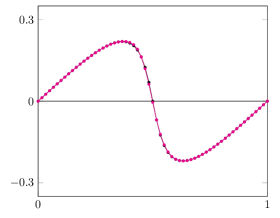
Figure 16: Exact ( ) and approximate ( ) solutions for $t_{\text{f}}=0.5$ the full RK₄+centered scheme (left) and the a posteriori strategy (right): the smooth solution case — benchmark 6.

We display in Figure 16-left the numerical approximation with the most accurate scheme (RK₄+centered) while we reproduce on the right side the approximation computed with the a posteriori strategy. We have checked that the table CSS has never been altered during the simulation, that is, computation have been achieved with the centered scheme and the RK₄ scheme in time due to the Péclet number. — benchmark 7. The last benchmark deals with a rough function (regarded to the characteristic mesh size) using the manufactured solution (11) but with $\delta=0.015$ corresponding to a steep variation we assimilate as a shock regarded to the small number of nodes $I=60$. We take constant physical parameters $u=1$ and $\kappa=5.5556$E$-03$ to obtain the cell Péclet number $Pe=3$. The simulation is again carried out until the final time $t_{\text{f}}=0.5$, corresponding to half a revolution

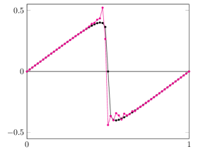
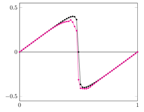
Figure 17: Exact ( ) and approximate ( ) solutions for $t_{\text{f}}=0.5$ the full RK₄+centered scheme (left) and the a posteriori strategy (right): the rough solution case — benchmark 7.

We display in Figure 17 the solution obtained with the “unlimited” RK₄+centered scheme (left) and the a posteriori method (right). Clearly, the steep gradient provokes oscillations when employing the low diffusive centered scheme while the introduction of the weak upwind scheme in some nodes (indicated with the red X on the figure) manages to stabilise the solution and strongly reduces the over- and under-shooting. Moreover the scheme in time on the node $i$ such that $\texttt{CSS}[i]=1$ (weak upwind) switch to the RK${}_{\text{D}}$ once $\texttt{CTS}[i]=1$ while the nodes where we maintain the original centered scheme $\texttt{CSS}[i]=0$ (centered upwind) use the RK₄ once $\texttt{CTS}[i]=0$. Notice that the number of nodes that have been cured is almost 3 or 4, i.e., less than 8% for a 60-nodes grid.

6 Conclusions and further work

We have developed a strategy to analyse and optimise the stability based, on the one hand, on the two-parameter family of continuous spectral curves that characterise the space discretization and, on the other hand, a two-parameter family of Runge-Kutta stability regions. Optimisation results from the inclusion of the spectral curves into the stability region with the help of the additional CFL parameter. We have detailed the procedure with the five-point finite difference method context but extension to other methods such as finite volume or finite elements methods could be considered. A hybrid time scheme as a function of the Péclet number have been proposed and analysed with the objective of providing the largest time step while preserving the stability. At last, we have presented an adaptation of the a posteriori strategy to handle the schemes in space and time to preserve both the accuracy and the stability, even for rough solutions, while we optimise the time step to reduce the computational effort.

References

- [1] A. Abdulle, Fourth order Chebyshev methods with recurrence relation, SIAM J. Sci. Comput. 23 (2002) 2042–2055.
- [2] A. Abdulle, A.A. Medovikov, Second order Chebyshev methods based on orthogonal polynomials, Numer. Math. 90 (2001) 1–18.
- [3] R. Ait-Haddou, New stability results for explicit Runge-Kutta methods, BIT Numer. Math. (2019) 585–612.
- [4] R. Araya, E. Behrens, R. Rodriguez, An adaptive stabilized finite element scheme for the advection-reaction-diffusion equation, Appl. Numer. Math. 54 (2005) 491–503.
- [5] A. Bourchtein, L. Bourchtein, Explicit finite difference schemes with extended stability for advection equations, J. Comput. Appl. Math. 236 (2012) 3591–3604.
- [6] J. Butcher, Numerical methods for Ordinary Differential Equations, Wiley, second ed., 2008.
- [7] N. M. Chadha, N. Madden, An optimal time-stepping algorithm for unsteady advection-diffusion problems, J. Comput. Appl. Math. 294 (2016) 57–77.
- [8] N. M. Chadha, N. Madden, A two-weight scheme for a time-dependent advection–diffusion problem, Lect. Notes Comput. Sci. Eng. 81 (2011) 99–108.
- [9] S. Clain, S. Diot, R. Loubère, A high-order finite volume method for hyperbolic systems: multi-dimensional optimal order detection (MOOD), J Comput Phys 230(10) (2011) 4028–50.
- [10] S. Diot, S. Clain, R. Loubère, Improved detection criteria for the multi-dimensional optimal order detection (MOOD) on unstructured meshes with very high-order polynomials, Comput Fluids 64 (2012) 43–63 .
- [11] S. Clain, R. Loubère, G. Machado, a posteriori stabilized sixth-order finite volume scheme for one-dimensional steady-state hyperbolic equations, Adv. Comput. Math. 44 (2018) 571-607.
- [12] V. G. Ferreira, F. A. Kurokawa, R. A. B. Queiroz, M. K. Kaibara, C. M. Oishi, J. A. Cuminato, A. Castelo, M. F. Tomé, S. McKee, Assessment of a high-order finite difference upwind scheme for the simulation of convection–diffusion problems, Int. J. Numer. Meth. Fluids 60 (2009) 1–26.
- [13] F. R. Gantmacher, The Theory of Matrices, Chelsea Publishing Co., NY 1960.
- [14] P. J. van der Houwen, B. P. Sommeijer, On the internal stability of explicit, m-stage Runge-Kutta methods for large m-values, Z. Angew. Math. Mech. 60 (1980) 479–485.
- [15] W. Hundsdorfer, J. Verwer, Numerical Solution of Time-Dependent Advection-Diffusion-Reaction Equations, Springer–Verlag Berlin Heidelberg, 2003.
- [16] D. I. Ketcheson, A. J. Ahmadia, Optimal Stability Polynomials for Numerical Integration of Initial Value Problems, Comm. App. Math. and Comp. Sci. 7 (10) (2012) 247–271.
- [17] T. Knopp, G. Lube, G. Rapin, Stabilized finite element methods with shock capturing for advection–diffusion problems, Comput. Methods Appl. Mech. Engrg. 191 (2002) 2997–3013.
- [18] G. V. Krivovichev, Optimized low-dispersion and low-dissipation two-derivative Runge-Kutta method for wave equations, J Appl Math Comput, 63 (2020) 787–811.
- [19] B. van Leer, Towards the Ultimate Conservative Difference Scheme, V. A Second Order Sequel to Godunov’s Method, J. Com. Phys., 32 (1979) 101–136.
- [20] X.-D. Liu, S. Osher, T. Chan, Weighted Essentially Non-oscillatory Schemes, J. Comput. Phys., 115 (1994) 200–212.
- [21] W. Riha, Optimal stability polynomials, Computing 9 (1972) 37–43.
- [22] M. Schlegel, O. Knoth, M. Arnold, R. Wolke, Multirate Runge-Kutta schemes for advection equations, J. Comput. Appl. Math. 226 (2009) 345–357.
- [23] L. M. Skorvtsov, Explicit stabilized Rung-Kutta methods, Comput. Math. Math. Phys., 51 (2011) 7 1153–1166.
- [24] L. N. Trefethen, Finite Difference and Spectral Methods for Ordinary and Partial Differential Equations, Unpublished Text, (1996) http://people.maths.ox.ac.uk/trefethen/pdetext.html.
- [25] R. Verfürth, A Review of a Posteriori Error Estimation and Adaptive Mesh-Refinement Techniques, Wiley–Teubner, Stuttgart, 1996.
- [26] C.-W. Shu, Total-variation diminishing time discretizations, SIAM J. Sci. Statist. Comput. 9 (1988), 1073–1084.
- [27] C.-W. Shu, S. Osher, Efficient implementation of essentially non-oscillatory shock-capturing schemes, J. Comput. Phys. 77 (1988) 439–471.
- [28] S. Wang, An a posteriori error estimate for finite element approximations of a singularly perturbed advection–diffusion problem, J. Comput. Appl. Math. 87 (1997) 227–242.
- [29] H. C. Yee, N. D. Sandham, M. J. Djomehri, Low dissipative high order shock-capturing methods using characteristic-based filters, J. Comput. Phys. 150 (1999) 199–238.