Copula Flows for Synthetic Data Generation

Abstract

The ability to generate high-fidelity synthetic data is crucial when available (real) data is limited or where privacy and data protection standards allow only for limited use of the given data, e.g., in medical and financial data-sets. Current state-of-the-art methods for synthetic data generation are based on generative models, such as Generative Adversarial Networks (GANs). Even though GANs have achieved remarkable results in synthetic data generation, they are often challenging to interpret. Furthermore, GAN-based methods can suffer when used with mixed real and categorical variables. Moreover, loss function (discriminator loss) design itself is problem specific, i.e., the generative model may not be useful for tasks it was not explicitly trained for. In this paper, we propose to use a probabilistic model as a synthetic data generator. Learning the probabilistic model for the data is equivalent to estimating the density of the data. Based on the copula theory, we divide the density estimation task into two parts, i.e., estimating univariate marginals and estimating the multivariate copula density over the univariate marginals. We use normalising flows to learn both the copula density and univariate marginals. We benchmark our method on both simulated and real data-sets in terms of density estimation as well as the ability to generate high-fidelity synthetic data.

1 Introduction

Machine learning is an integral part of daily decision-support systems, ranging from personalised medicine to credit lending in banks and financial institutions. The downside of such a pervasive use of machine learning is the privacy concern associated with the use of personal data  [Elliot and Domingo-Ferrer, 2018]. In some applications, such as medicine, sharing data with privacy in mind is fundamental for advancing the science [Beaulieu-Jones et al., 2019]. However, the available data may not be sufficient to realistically train state-of-the-art machine learning algorithms. Synthetic data is one way of mitigating this challenge.

Current state-of-the-art methods for synthetic data generation, such as Generative Adversarial Networks (GANs) [Goodfellow et al., 2014], use complex deep generative networks to produce high-quality synthetic data for a large variety of problems [Choi et al., 2017, Xu et al., 2019]. However, GANs are known to be unstable and delicate to train [Arjovsky and Bottou, 2017]. Moreover, GANs are also notoriously difficult to interpret, and finding an appropriate loss function is an active area of research [Wang et al., 2019]. Another class of models, variational auto encoders (VAEs) [Kingma and Welling, 2013, Rezende and Mohamed, 2015] have also been used to generate data, although their primary focus is finding a lower-dimensional data representation. While deep generative models, such as VAEs and GANs, can generate high-fidelity synthetic data, they are both difficult to interpret. Due to the complex composition of deep networks, it is nearly impossible to characterise the impact of varying weights on the density of the generated data. For VAEs, a latent space may be used to interpret different aspects of the data.

In this work, we focus on probabilistic models based on copulas. Sklar showed that any multivariate distribution function can be expressed as a function of its univariate marginals and a copula [Sklar, 1959]. However, estimating copulas for multivariate mixed data types is typically hard, owing to 1) very few parametric copulas have multivariate formulations and 2) copulas are not unique for discrete or count data [Nikoloulopoulos and Karlis, 2009]. To address the first challenge, the current standard is to use a pairwise copula construction Aas et al. [2009], which involves two steps identifying the pair copula and a tree structure defining pairwise relationship [Elidan, 2010, Lopez-paz et al., 2013, Czado, 2010, Chang et al., 2019].

In this paper, we propose a probabilistic synthetic data generator that is interpretable and can model arbitrarily complex data-sets. Our approach is based on normalising flows to estimate copulas. We show that our model is flexible enough to learn complex relationships and does not rely on explicit learning of the graph or parametric bivariate copulas. Figure 1 illustrates the flexibility of our proposed method by modelling copula with a complex structure. We are not aware of any copula based method able to learn the copula shown in Figure 1 a).

To deal with count data, we propose a modified spline flow [Durkan et al., 2019] as a continuous relaxation of discrete probability mass functions. This formulation allows us to build complex multivariate models with mixed data types that can learn copula-based flow models, which can be used for the following tasks:

• Synthetic data generation: Use the estimated model to generate new data-sets that have a distribution similar to the training set.

• Inferential statistics: When the copula has learned the relationship between the variables correctly, one can change the marginals to study the effects of change. For example, if we estimated a copula flow based on a UK dataset with age as one of the variables, we can modify the marginal of the age distribution to generate synthetic data for a different country. To generate data for Germany, we would use Germany’s age distribution as a marginal for the data-generating process.

• Privacy preservation: The data generated from the copula flow model is fully synthetic, i.e., the generator does not rely on actual observations for generating new data. One can perturb the generated data based on differential privacy mechanisms to prevent privacy attacks based on a large number of identical queries.

Figure 1: Learning the joint and marginal distributions for ‘2 rings’ data. This figure demonstrates how copulas and marginals can be combined to obtain complex joint distributions. The copula associated with the ‘2 rings’ distribution cannot be modelled by any standard bi-variate copula, whereas our proposed copula flow method can learn this structure.

2 Background

We denote the domain of a function $F$ by $\mathbf{dom}({F})$ and range by $\mathbf{ran}({F})$. We use capital letters $X,Y$ to denote random variables and lower case $x,y$ to represent their realisations. Bold symbols $\boldsymbol{X}=[X_{1},\ldots,X_{d}]$ and corresponding $\boldsymbol{x}=[x_{1},\ldots,x_{d}]$ represent vectors of random variables and their realisations, respectively. We denote the distribution function (also known as the Cumulative Distribution Function (CDF)) of a random variable $X$ by $F_{X}$, and the corresponding Probability Density Function (PDF) by $f_{X}$. Such functions play an important role in copula theory. If we map a random variable through its own distribution function we get an uniformly distributed random variable-$\text{Uniform}\left[0,1\right]$ or uniform marginal. This is known as probability integral transform [David and Johnson, 1948]. A copula is a relationship, literally a link, between uniform marginals obtained via the probability integral transform [Nelsen, 2006]. Two random variables are independent if the joint copula of their uniform marginals is independent. Conversely, random variables are linked via their copulas.

2.1 Copulas

For a pair of random variables, the marginal CDFs $F_{X},F_{Y}$ describe how each variable is individually distributed. The joint CDF $F_{X,Y}$ tells us how they are jointly distributed. Sklar’s seminal result [Sklar, 1959] allows us to write the joint CDF as a function of the univariate marginals $F_{X}$ and $F_{Y}$, i.e.,

$$F_{X,Y}(X,Y) =C\left(U_{X},U_{Y}\right)=C\left(F_{X}(X),F_{Y}(Y)\right),$$ (1)

where $C$ is a copula. Here, the uniform marginals are obtained by the probability integral transform, i.e., $U_{X}=F_{X}(X)$ and $U_{Y}=F_{Y}(Y)$.

Copulas describe the dependence structure independent of the marginal distribution, which we exploit for synthetic data generation; especially in privacy preservation, where we perturb data samples by another random process, e.g., the Laplacian mechanism [Dwork and Roth, 2013]. This changes the marginal distribution but crucially it does not alter the copula of the original data.

For continuous marginals $F_{X}$ and $F_{Y}$, the copula $C$ is unique, whereas for discrete marginals it is unique only on $\mathbf{ran}({F_{X}})\times\mathbf{ran}({F_{Y}})$. A corollary of Sklar’s theorem is that $X$ and $Y$ are independent if and only if their copula is an independent copula, i.e., $C(F_{X}(X),F_{Y}(Y))=F_{X}(X)\,F_{Y}(Y)$.

2.2 Generative Sampling

We can use the constructive inverse of Sklar’s theorem for building a generative model. The key concept is that the inverse of the probability integral transform, called inverse transform sampling, allows us to generate random samples starting from a uniform distribution. The procedure to generate a random sample $x$ distributed as $F_{X}$ is to first sample a random variable $u\sim\text{Uniform}\left[0,1\right]$ and second to set $x:=F_{X}^{(-1)}(u)$. Here, the the function $F^{(-1)}$ is a quasi-inverse function.

Definition 2.1 (Quasi-inverse function)

Let $F$ be a CDF. Then the function $F^{(-1)}$ is a quasi-inverse function of $F$ with domain $[0,1]$ such that $F(F^{(-1)}(y))=y\quad\forall\,y\in\mathbf{ran}({F})$ and $F^{(-1)}(y)=\inf\left\{x|F(x)\geq y\right\}\forall\,x\in\mathbf{dom}({F}),\,\text{and}\,y\notin\mathbf{ran}({F})$. For strictly monotonically increasing $F$, the quasi-inverse becomes the regular inverse CDF $F^{-1}$ [Nelsen, 2006].

The inverse function, also called as the quantile function, maps a random variable from a uniform distribution to $F$-distributed random variables, i.e., $X=F^{-1}(U)$ or $F^{-1}:\text{Uniform}\left[0,1\right]\rightarrow\mathbf{ran}({F})$. Hence, we can present the problem of synthetic data generation as the problem of estimating the (quasi)-inverse function for the given data.

To generate samples from $F_{X}$ using a copula-based model, we start with a pair of uniformly distributed random variables, then pass them through inverse of the copula CDF to obtain correlated uniform marginals; see Figure 2 b). Note that the copulas are defined over uniform marginals, i.e., the random variables are uniformly distributed. We use the correlated univariate marginals to subsequently generate $F$-distributed random variables via inverse transform sampling; see Figure 2 c). Hence, if we can learn the CDFs for the copula as well as the marginals, we can then combine these two models to generate correlated random samples that are distributed similar to the training data. The procedure is illustrated in Figure 2.

Figure 2: Copula flow generative model. Left: We start with uniformly distributed independent variable samples. These samples are passed through the copula flow network to generate correlated uniformly distributed random variables (middle). The correlated variables are transformed to the desired distribution by using univariate marginal flows $\mathcal{F}_{X}$ (right).

3 Copula Flows

The inverse function used to generate synthetic data can be described as a flow function $\mathcal{F}_{X}\approx F_{X}^{(-1)}$ that transforms a uniform random variable $U$ into $X\sim F_{X}$, see Figure 2. We can interpret the (quasi)-inverse function as a normalising flow [Tabak and Vanden-Eijnden, 2010, Rezende and Mohamed, 2015, Papamakarios et al., 2019] that transforms a uniform density into the one described by the copula distribution function $C$. We refer it as copula flow.

3.1 Normalising Flows

Normalising flows are compositions of smooth, invertible mappings that transform one density into another [Rezende and Mohamed, 2015, Papamakarios et al., 2019]. The approximation in $\mathcal{F}_{X}\approx F_{X}^{(-1)}$ indicates that we are estimating a (quasi) inverse distribution function by using a flow function $\mathcal{F}_{X}$. If we learn the true CDF $F_{X}$, we have

$$F_{X}(x)=\mathcal{F}_{X}^{-1}(x)=u,\,u\sim\text{Uniform}\left[0,1\right],\quad\forall x\in\mathbf{dom}({F_{X}}),$$ (2)

due to uniqueness of the CDF. An advantage of the normalising flow formulation is that we can construct arbitrarily complex maps as long as they are invertible and differentiable.

Consider an invertible flow function $\boldsymbol{\mathcal{F}}:\mathbb{R}^{D}\rightarrow\mathbb{R}^{D}$, which transforms a random variable as $\boldsymbol{X}=\boldsymbol{\mathcal{F}}(\boldsymbol{U})$. By using the change of variables formula, the density $f_{\boldsymbol{X}}$ of variable $\boldsymbol{X}$ is obtained as

$$f_{\boldsymbol{X}}(\boldsymbol{X}) =f_{\boldsymbol{U}}\left(\mathcal{F}^{-1}(\boldsymbol{X})\right)\left|\operatorname{det}\left(\tfrac{\partial\boldsymbol{\mathcal{F}}^{-1}(\boldsymbol{X})}{\partial\boldsymbol{X}}\right)\right|=\,\left|\operatorname{det}\left(\tfrac{\partial\boldsymbol{\mathcal{F}}^{-1}(\boldsymbol{X})}{\partial\boldsymbol{X}}\right)\right|,$$ (3)

where $f_{\boldsymbol{U}}\left(\mathcal{F}^{-1}(\boldsymbol{X})\right)=f_{\boldsymbol{U}}(\boldsymbol{U})=1.0$, since $f_{\boldsymbol{U}}=\text{Uniform}\left[0,1\right]$.

For the copula flow model, we assume that the copula density $c$ of the copula CDF $C$ exists. Starting with the bivariate case for random variables $X,Y$, we compute the density $f_{XY}$ via the partial derivatives of the $C$, i.e.,

$$f_{XY} =\frac{\partial^{2}C(F_{X},F_{Y})}{\partial F_{X}\partial F_{Y}}=c_{XY}(F_{X},F_{Y})\,f_{X}\,f_{Y}.$$ (4)

We can generalise this result to the joint density $f_{\boldsymbol{X}}(\boldsymbol{X})$ of a $d$-dimensional random vector $\boldsymbol{X}=[X_{1},\ldots,X_{d}]$ as

$$f_{\boldsymbol{X}} =\underbrace{c_{\boldsymbol{X}}(F_{X_{1}},\ldots,F_{X_{d}})\vphantom{\prod\nolimits_{k=1}^{d}}}_{\text{copula density}}\,\underbrace{\prod\nolimits_{k=1}^{d}f_{X_{k}}}_{\text{marginal density}}.$$ (5)

To construct the copula-based flow model, we begin with rewriting the joint density $f_{\boldsymbol{X}}$ in (5) in terms of marginal flows $\mathcal{F}$ and the joint copula flow $\mathcal{C}_{\boldsymbol{X}}$. We then obtain

$$f_{\boldsymbol{X}}(\boldsymbol{X}) =\left|\operatorname{det}\left(\tfrac{\partial\mathcal{C}_{\boldsymbol{X}}^{-1}(\boldsymbol{U}_{\boldsymbol{X}})}{\partial\boldsymbol{U}_{\boldsymbol{X}}}\right)\right|\prod\nolimits_{k=1}^{d}\left|\tfrac{\partial\mathcal{F}_{X_{k}}^{-1}(X_{k})}{\partial X_{k}}\right|,$$ (6)

where $\mathcal{C}_{\boldsymbol{X}}$ is the copula flow function and $\mathcal{F}_{X_{1}},\ldots,\mathcal{F}_{X_{d}}$ are marginal flow functions; see Appendix A for the detailed derivation. Even though the copula itself is defined on independent univariate marginals functions, we use $X$ in the notation to emphasise that these univariates are obtained by inverting the flow $U_{X_{k}}=\mathcal{F}^{-1}_{X_{k}}(X_{k})$ for marginals.

Given a data-set $\{\boldsymbol{x}_{1},\ldots,\boldsymbol{x}_{N}\}$ of size $N$, we train the flow by maximising the total log-likelihood $\mathcal{L}=\log f_{\boldsymbol{X}}(\boldsymbol{x})=\sum_{n=1}^{N}\log f_{\boldsymbol{X}}(\boldsymbol{x}_{n})$ with respect to the parametrisation of flow function $\mathcal{F}$. The log-likelihood can be written as the sum of two terms, namely

$$\mathcal{L} =\mathcal{L}_{\mathcal{C}_{\boldsymbol{X}}}+\mathcal{L}_{\boldsymbol{\mathcal{F}}}=\mathcal{L}_{\mathcal{C}_{\boldsymbol{X}}}+\sum\nolimits_{k=1}^{d}\mathcal{L}_{X_{k}}.$$ (7)

The copula flow log-likelihood $\mathcal{L}_{\mathcal{C}_{\boldsymbol{X}}}$ depends on the marginals flows. Hence, we train the marginal flows first and then the copula flow. The gradients of both log-likelihood terms are independent as they are separable. The procedure of first training the marginals before fitting copula models is standard in the copula literature and yields better performance and numerical stability [Joe, 2005].

3.2 Copula Flows

Copula is a CDF defined over uniform marginals, i.e., $\text{Uniform}\left[0,1\right]^{d}\rightarrow\text{Uniform}\left[0,1\right]$. We can use the inverse of this CDF to generate samples via inverse transform sampling. For the multivariate case, we can use the conditional generation procedure [Hansen, 1994]. Let $\boldsymbol{U}_{\boldsymbol{X}}=[U_{X_{1}},\ldots,U_{X_{d}}]$ be a random vector with copula $\boldsymbol{C}_{\boldsymbol{X}}$, and $\boldsymbol{U}=U_{1},\ldots,U_{d}$ be i.i.d. $\text{Uniform}\left[0,1\right]$ random variables. Then the multivariate flow transform $\boldsymbol{U}_{X}:=\boldsymbol{\mathcal{C}}_{\boldsymbol{X}}(\boldsymbol{U})$ can be defined recursively as

$$U_{X_{1}} :=\mathcal{C}_{X_{1}}(U_{1}),\quad U_{X_{k}}:=\mathcal{C}_{X_{k|1,\ldots k-1}}\left(U_{k}|U_{X_{1},\ldots,X_{k-1}}\right),\quad 2\leq k\leq d,$$ (8)

where $\mathcal{C}_{X_{k|1,\ldots k-1}}=C^{-1}_{X_{k|1,\ldots k-1}}$ is the flow function conditioned on all the variables $U_{X_{1}},\ldots,U_{X_{k-1}}$. The key concept is the interpretation of the inverse of the (normalising) copula flow $\mathcal{C}_{\boldsymbol{X}}^{-1}$ as a conditional CDF. Moreover, we estimate $\mathcal{C}_{X_{k|1,\ldots k-1}}$ recursively, with one dimension at a time, via a neural spline network [Durkan et al., 2019]. The conditioning variables, $X_{1},\ldots X_{k-1}$ are input to the network that outputs spline parameters for the flow $\mathcal{C}_{X_{k|1,\ldots k-1}}$. The procedure above is similar to auto-regressive density estimators [Papamakarios et al., 2017, 2019] with Masked Autoregressive Flow (MAF) structure [Germain et al., 2015, Papamakarios et al., 2017]. Similar to MAF we can stack such multiple flows to create flexible multivariate copula flow $\boldsymbol{\mathcal{C}}_{\boldsymbol{X}}$. In the copula literature this multivariate extension is convenient for Archimedean copulas [Nelsen, 2006], where the generators for such copulas can be interpreted as conditional flow functions.

3.3 Univariate Marginal Flows

To estimate univariate marginals, we can use both parametric and non-parametric density estimation methods as the dimensionality is not a challenge. However, for training the copula, we require models that can be inverted easily to obtain uniform marginals, i.e., we need to have a well-defined CDF for the methods we employ for the density estimation. Simultaneously, we need a model that can be used for generating data via inverse transform sampling. We propose to use monotone rational quadratic splines, neural spline flows (NSF) [Durkan et al., 2019]. With the a sufficiently dense spline, i.e., a large number of knot positions, we can learn arbitrarily complex marginal distributions. As we directly attempt to learn the quasi-inverse function $\mathcal{F}:\text{Uniform}\left[0,1\right]\,\rightarrow\,\mathbf{ran}({F})$, where $F$ is the true CDF, a single parameter vector $\boldsymbol{\theta}_{d}=[\boldsymbol{\theta}_{d}^{w},\boldsymbol{\theta}_{d}^{h},\boldsymbol{\theta}_{d}^{s}]$ describing the width, height and slope parameters, respectively, is sufficient. We document the details of the proposed spline network in Appendix E

4 Discrete Data Modelling

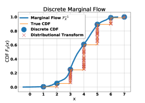
Figure 3: Illustration of discrete marginal flow for three discrete classes. The marginal flow (blue) gives discrete samples when rounded up. The distributional transform is uniform along the vertical line of the true CDF (orange).

Modelling mixed variables via normalising flows is challenging [Onken and Panzeri, 2016, Ziegler and Rush, 2019, Tran et al., 2019]. Discrete data poses challenges for both copula learning as well as learning flow functions. For marginals, i.e., univariate flow functions, the input is a uniform distribution continuous in $[0,1]$, whereas the output is discrete and hence discontinuous. For copula learning, we need uniform marginals for the given training data. With discrete inputs to the inverse flow function (CDF), the output is discontinuous in $[0,1]$.

4.1 Marginal Flows for Discrete/Count Data

We first focus on learning the univariate flow maps, i.e., marginal learning. Ordinal variables have a natural order, which we can use directly. For categorical data, we propose to assign each class a unique integer in $\{0,\ldots,n-1\}$, where $n$ is the number of classes. We define a CDF over these integer values. As this assignment is not unique, the same category assignment needs to be maintained for training and data generation.

For discrete data generation, we round the data output of the flow function to the next higher integer, i.e., we can consider random variable $Y=\text{ceil}(X)$. However, this procedure does not yield a valid density. To ensure that that the samples are properly discretised, we use a quantised distribution [Salimans et al., 2019, Dillon et al., 2017] so that density learning can be formulated as a quantile learning procedure.

We assign a quantile range for a given class or ordinal integer. We use the same spline-based flow functions as the one used for continuous marginals, but with quantisation as the last step. The advantage of this discrete flow is that our quasi-inverse, i.e., the flow function is a continuous and monotonic function, which can be trained by maximising the likelihood. Figure 3 shows the spline-based flow function learned for a hypergeometric distribution. The continuous flow function (blue curve in Figure 3) learned for the discrete marginal, light orange step function in Figure 3, allows us to generate discrete data via inverse transform sampling.

4.2 Mixed Variable Copulas

However, the inverse of this flow function, i.e., the CDF of the marginal, results in discontinuous values at the locations of the training inputs (blue circles in Figure 3). Copulas are unique and well defined only for continuous univariate marginals. An elegant way to find continuous univariate marginals for the discrete variable is via the distributional transform [Rüschendorf, 2009].

Definition 4.1 (Distributional Transform)

Let $X\sim F_{X}$. The modified CDF is defined as

$$F_{X}(x,\lambda):=\mathrm{Pr}(X<x)+\lambda\mathrm{Pr}(X=x).$$ (9)

Let $V$ be uniformly distributed independent of $X$. Then the distributional transform $X\rightarrow U$ of $X$ is

$$u:=\mathcal{F}^{-1}_{X}(x)=F_{X-}(x)+V(F_{X}(x)-F_{X-}(x)),$$ (10)

where $F_{X-}(x)=\mathrm{Pr}(X<x)$, $F_{X}(x)=\mathrm{Pr}(X\leq x)$ and $\mathrm{Pr}(X=x)=F_{X}(x)-F_{-}(x)$. With this, we have $U\,\sim\text{Uniform}\left[0,1\right]$ and $X=\mathcal{F}_{X}(U)\,a.s.$ [Rüschendorf, 2009].

This distributional transform behaves similar to the probability integral transform for continuous distributions, i.e., a discrete random variable $X$ mapped through the distributional transform gives an uniform marginal. However, unlike for continuous variables, the distributional map is stochastic and hence not unique. With the distributional transform, the copula model does not need a special treatment for discrete variables; see section 2 in [Rüschendorf, 2009] for details. In Figure 3, the red cross marks show the values from distributional transform. All samples along the $y$-axis that share same $x$-value. With the distributional transform and marginal splines, the copula flow model leverages recent advances in normalising flows to learn arbitrarily complex distributions. Moreover, we can show that:

Theorem 4.2

A copula flow is a universal density approximator.  Proof: Appendix D.1.

Hence, we can learn a model to generate any type of data, discrete or continuous, with the proposed copula flow model. This property holds true when the flow network converges to the inverse function.

5 Related Work

The Synthetic Data Vault (SDV) project [Patki et al., 2016] is very close in spirit of this paper. In the SDV, the univariate marginals are learned by using a Gaussian mixture model, and the multivariate copula is learned as a Gaussian copula. Unlike flow-based estimation, proposed in this work, copula-based models typically follow a two-step procedure, the pair-copula construction or vine copulas, by first constructing a pairwise dependence structure and then learning pair-copulas for it [Aas et al., 2009]. Copula Bayesian networks [Elidan, 2010] use conditional copulas and learn a Bayesian network over the variables. In [Chang et al., 2019], the authors propose to use Monte-Carlo tree search for finding the network structure. Such models have limited flexibility, e.g., no standard copula model can learn the structure in figure 1, which our model (copula flow) can learn.

GAN-based methods are the workhorse of the majority of recent advances in the synthetic data generation, e.g., the conditional GAN [Xu et al., 2019], builds a conditional generator to tackle mixed-variable types, whereas the tableGAN [Park et al., 2018] builds GANs for privacy preservation. Unlike the tableGAN, the PATE-GAN [Jordon et al., 2019] produces synthetic data with differential privacy guarantees. Data generators for medical records [Che et al., 2017, Choi et al., 2017] are also based on GANs.

Normalising flow methods have had very rapid growth in terms of the continuous improvements on benchmarks introduced by [Papamakarios et al., 2017]. Our work relies heavily on the NSF [Durkan et al., 2019, Müller et al., 2019]. Instead of training models with a likelihood loss, in [Nash and Durkan, 2019], the authors use auto-regressive energy models for density estimation. While most methods either rely on coupling [Dinh et al., 2015, 2019] or auto-regressive [Papamakarios et al., 2017, Kingma et al., 2016] models, transformation networks Oliva et al. [2018] use a combination of both. The neural auto-regressive flows [Huang et al., 2018], which have monotonic function guarantees, can be used as a drop-in replacement for the spline-based copula network used in this paper.

6 Experiments

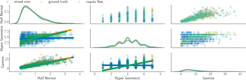
Figure 4: Mixed variable copula learning: joint marginals, joint scatter plots, regression plots. Fitting a mixed type vine [Onken and Panzeri, 2016]. $X_{2}$ is a discrete Hyper geometric, $X_{1}$ is Half Normal, and $X_{3}$ is Gamma distributed. Pairwise copulas $\left(X_{1}\text{ and }X_{2}\right)$ Gaussian, $\left(X_{2}\text{ and }X_{3}\right)$ Clayton, $\left(X_{1}\text{ and }X_{3}\right)$ Gumbel. The diagonal plots show the marginals for each variable, whereas the upper triangle shows joint scatter plots. The lower triangle shows regression plots for each variable. Here, we overlay a linear regression fit and data for the pair of variables. For continuous variables $X_{1}$ and $X_{3}$ all three methods produce regression lines similar to each other. For relations between discrete and continuous variables, the copula flow and the ground truth align. However, for both discrete to continuous relations, the mixed vine fails to capture the relation as evident by the misaligned linear regression fit.

Our proposed copula flow can learn copula models with continuous and discrete variables. This allows us to use the model to learn complex relations in tabular data as well.

Mixed Variable Copula Learning

We start with an illustrative example by constructing a generative model with discrete and continuous variables. We demonstrate that the copula flow model can indeed learn the structure as well as the marginal densities. We construct a vine model with three different marginals: 1) $X_{1}$, continuous, Half Normal; 2) $X_{2}$ discrete, hypergeometric; 3) $X_{3}$, continuous, Gamma. Since the copula describes a symmetric relationship, we have three different bivariate relations between three variables. We assign three widely used bivariate copulas: a Gaussian for $X_{1}$ and $X_{2}$, a Clayton for $X_{2}$ and $X_{3}$, and a Gumbel copula for $X_{1}$ and $X_{3}$. This model is inspired by the mixed vine data model described in [Onken and Panzeri, 2016], where authors propose to build a likelihood using CDFs and vine for mixed data. We use this model as a baseline for comparison. The copula flow can learn all three marginals, which are plotted along the diagonal of Figure 4, while the mixed vine copula struggles a bit (second row, second column). The copula flow also successfully learns copulas between discrete and continuous variables, as evident by the linear regression line in the lower half of the plots in Figure 4. Both the mixed vine model [Onken and Panzeri, 2016] and the copula flow can learn the continuous copula well as evident by the left lowermost regression plot, but the mixed vine copula struggles with mixed variable copulas (third row, second column of Figure 4). Scatter plots in the upper diagonal show that the samples from mixed vine model are more spread out while copula flow samples align with the true samples.

Density Estimation

For density estimation, we compare the performance against the current state of the art neural density estimators. The standard benchmark introduced by [Papamakarios et al., 2017] modifies the original data with discrete marginals. For example, in the UCI power data-set, the authors add a uniform random noise to the sub-metering columns. This is equivalent to using the distributional transform, Definition 4.1, with a fixed seed. These ad-hoc changes defeat the purpose of interpretability and transparency. However, to maintain the exact comparison across different density estimators we keep the data, training, test, and validation splits exactly as in [Papamakarios et al., 2017], with the code provided by [Oliva et al., 2018]. We use CDF splines flow for estimating the marginals, which is equivalent to estimating the model with an independence copula. We obtain the univariate uniform marginals by inverting the flow, and then fit a copula flow model to obtain the joint density. We summarise the density estimation results in Table 1. The marginal likelihood scores ignore the relationships amongst the variables, whereas the copula likelihood shows information gained by using copula. The joint likelihood can be expressed as sum of marginal and copula likelihoods, see (7) The copula flow based model achieves a performance that is close to the state of the art. Further improvements may be achieved by fine tuning the copula flow structure as the marginal CDFs are close to the empirical CDF as verified by using the Kolmogorov-Smirnov (KS) test; see Appendix B

Model	Power	Gas	Hepmass	Miniboone
FFJORD	$0.46\pm 0.01$	$8.59\pm 0.12$	$-14.92\pm 0.08$	$-10.43\pm 0.04$
RQ-NSF (AR) [Durkan et al., 2019]	$0.66\pm 0.01$	$13.09\pm 0.02$	$-14.01\pm 0.03$	$-9.22\pm 0.48$
MAF [Papamakarios et al., 2017]	$0.45\pm 0.01$	$12.35\pm 0.02$	$-17.03\pm 0.02$	$-10.92\pm 0.46$
Marginal Flows $\mathcal{F}$	$-0.80\pm 0.02$	$-6.67\pm 0.02$	$-26.42\pm 0.05$	$-53.17\pm 0.06$
Copula Flow $\mathcal{C}$	$1.39\pm 0.03$	$15.6\pm 0.67$	$5.4\pm 0.10$	$37.77\pm 0.21$
Joint Model $\mathcal{C}\,+\,\mathcal{F}$	$0.59\pm 0.03$	$8.05\pm 0.68$	$-19.6\pm 0.12$	$-14.83\pm 0.21$

Table 1: Test log-likelihoods (nats) on density estimation benchmarks. Exact replication of the dataset and splits as provided by [Papamakarios et al., 2017].

Synthetic Data Generation

Estimating the performance of data generators is a challenging process [Theis et al., 2016]. Merely having very high likelihood on the training or test set is not necessarily the best metric. One measure to look at is the machine learning efficacy of the generated data, i.e., whether can we use the synthetic data to effectively perform machine learning tasks (e.g., regression or classification), which we wished to accomplish with the true data [Xu et al., 2019, Jordon et al., 2019]. Here, we test the synthetic data generator using the framework introduced in [Xu et al., 2019]. The copula flow model can capture the relations between different variables while learning a density model as it is evident by the high scores in the ML tasks benchmark; see Table 2. For Gaussian mixture (GM) based models, the copula flow model performs very close to the ‘Identity’ transform, which uses the true data. This indicates a high similarity of the true and the synthetic data-set. For real data, the model performs very close to the current state of the art [Xu et al., 2019] for classification tasks and outperforms it on regression tasks on aggregate. The quality of learned CDFs is assessed by using the KS test; see Appendix B.

	GM Sim.				BN Sim.				Real
Method	$\mathcal{L}_{syn}$	$\mathcal{L}_{test}$			$\mathcal{L}_{syn}$	$\mathcal{L}_{test}$			clf	reg
Identity	-2.61	-2.61			-9.33	-9.36			0.743	0.14
CLBN [Che et al., 2017]	-3.06	7.31			-10.66	-9.92			0.382	-6.28
PrivBN [Zhang et al., 2017]	-3.38	-12.42			-12.97	-10.90			0.225	-4.49
MedGAN [Choi et al., 2017]	-7.27	-60.03			-11.14	-12.15			0.137	-8.80
VeeGAN [Srivastava et al., 2017]	-10.06	-4.22			-15.40	-13.86			0.143	-6.5e6
TableGAN [Park et al., 2018]	-8.24	-4.12			-11.84	-10.47			0.162	-3.09
TVAE [Xu et al., 2019]	-2.65	-5.42			-6.76	-9.59			0.519	-0.20
CTGAN [Xu et al., 2019]	-5.72	-3.40			-11.67	-10.60			0.469	-0.43
CopulaFlow	-3.17	-2.98			-10.51	-9.69			0.431	-0.18

Table 2: Performance of the copula flow models for synthetic data generation. We benchmark by using the synthetic data to perform the machine learning (ML) task, classification or regression, associated with the data-set. The metric is generated for the original test data. Gaussian mixture (GM) and Bayesian network (BN) simulations correspond to data generated from known GM or BN models. Log-likelihoods $\mathcal{L}_{syn}$ of the true model given synthetic data and $\mathcal{L}_{test}$ of the generative model given the test data are shown. All values except the copula flow are from the framework in [Xu et al., 2019].

7 Conclusion

In this work we proposed a new probabilistic model to generate high fidelity synthetic data. Our model is based on copula theory which allows us to build interpretable and flexible model for the data generation. We used distributional transform to address the challenges associated with learning copulas for discrete data. Experimental results show that our proposed model is capable of learning mixed variable copulas required for tabular data-sets. We show that synthetic data generated from a variety of real data-sets is capable of capturing the relationship amongst the mixed variables. Our model can be extended to generate data with differential privacy guarantees. We consider this as an important extension and future work. Moreover, our copula flow model can also be used, where copula models are used, e.g., in finance and actuarial science.

Broader Impact

Copula based density models are interpretable, as combination of individual behaviour and their joint tendencies independent of individual behaviour. Hence, these models are used in financial and insurance modelling, where interpretable models are needed for regulatory purposes. Appeal for synthetic data stems from inherent data privacy achieved by the model as it hides true data. However, the current implementation is still prone to privacy attacks as one can use a large number of queries to learn the statistics from the model, i.e., private data may leak through the synthetic data generated by the proposed model. Copula models are typically governed by a small number of parameters, whereas the copula flow model has very large deep network. This can pose a challenge even if the output of the network is interpretable.

Appendix A Flow Model

We can derive the flow-based likelihood by starting from the generative procedure for the samples. We start with a $d$-dimensional independently distributed random vector $\boldsymbol{U}\sim\text{Uniform}\left[0,1\right]^{d}$ and map it through the copula flow $\mathcal{C}_{\boldsymbol{X}}$ to obtain the random vector $\boldsymbol{U}_{X}=\mathcal{C}_{\boldsymbol{X}}(\boldsymbol{U})$. The joint vector is then mapped through the marginal flows $\boldsymbol{\mathcal{F}}_{\boldsymbol{X}}$ to obtain a random vector $\boldsymbol{X}=\mathcal{F}_{\boldsymbol{X}}(\boldsymbol{U}_{X})$. The combined formulation can be written as a composition of two flows to obtain $\boldsymbol{X}=\mathcal{F}_{\boldsymbol{X}}\left(\mathcal{C}_{\boldsymbol{X}}(\boldsymbol{U})\right)$, which is also a valid flow function [Rezende and Mohamed, 2015].

The likelihood for this flow function can be written as

$$\boldsymbol{f}_{\boldsymbol{X}}(\boldsymbol{X}) =\boldsymbol{f}_{\boldsymbol{U}_{\boldsymbol{X}}}(\boldsymbol{\mathcal{F}}_{\boldsymbol{X}}^{-1}(\boldsymbol{X}))\,\left|\mathrm{det}\left(\frac{\partial\boldsymbol{\mathcal{F}}_{\boldsymbol{X}}^{-1}(\boldsymbol{X})}{\partial\boldsymbol{X}}\right)\right|.$$ (11)

The marginal flows are independent for each dimension of the random vector $\boldsymbol{X}$. Hence, the determinant can be expressed as a product of the diagonal terms to obtain the likelihood

$$\boldsymbol{f}_{\boldsymbol{X}}(\boldsymbol{X}) =\boldsymbol{f}_{\boldsymbol{U}_{\boldsymbol{X}}}(\boldsymbol{\mathcal{F}}_{\boldsymbol{X}}^{-1}(\boldsymbol{X}))\,\prod_{i=1}^{d}\left|\left(\frac{\partial\mathcal{F}_{X_{i}}^{-1}(x_{i})}{\partial x_{i}}\right)\right|.$$ (12)

The quantity $\boldsymbol{f}_{\boldsymbol{U}_{\boldsymbol{X}}}(\boldsymbol{\mathcal{F}}_{\boldsymbol{X}}^{-1}(\boldsymbol{X}))$ is essentially the flow likelihood for the copula density, which we can write as

$$\boldsymbol{f}_{\boldsymbol{U}_{\boldsymbol{X}}}(\boldsymbol{\mathcal{F}}_{\boldsymbol{X}}^{-1}(\boldsymbol{X})) =\boldsymbol{f}_{\boldsymbol{U}_{\boldsymbol{X}}}\left(\boldsymbol{\mathcal{C}}_{\boldsymbol{X}}(\boldsymbol{U})\right)$$ (13)

$$=\boldsymbol{f}_{\boldsymbol{U}}(\boldsymbol{\mathcal{C}}_{\boldsymbol{X}}^{-1}(\boldsymbol{U}_{\boldsymbol{X}}))\,\left|\mathrm{det}\left(\frac{\partial\boldsymbol{\mathcal{C}}_{\boldsymbol{X}}^{-1}(\boldsymbol{U}_{\boldsymbol{X}})}{\partial\boldsymbol{U}_{\boldsymbol{X}}}\right)\right|$$ (14)

$$=\left|\mathrm{det}\left(\frac{\partial\boldsymbol{\mathcal{C}}_{\boldsymbol{X}}^{-1}(\boldsymbol{U}_{\boldsymbol{X}})}{\partial\boldsymbol{U}_{\boldsymbol{X}}}\right)\right|,$$ (15)

where $f_{\boldsymbol{U}}\left(\mathcal{C}_{\boldsymbol{X}}^{-1}(\boldsymbol{U}_{\boldsymbol{X}})\right)=f_{\boldsymbol{U}}(\boldsymbol{U})=1.0$, since $f_{\boldsymbol{U}}=\text{Uniform}\left[0,1\right]$. Using the the copula likelihood in (11) in the total likelihood (15) yields

$$\boldsymbol{f}_{\boldsymbol{X}}(\boldsymbol{X}) =\left|\mathrm{det}\left(\frac{\partial\boldsymbol{\mathcal{C}}_{\boldsymbol{X}}^{-1}(\boldsymbol{\mathcal{F}}_{\boldsymbol{X}}^{-1}(\boldsymbol{X}))}{\partial\boldsymbol{\mathcal{F}}_{\boldsymbol{X}}^{-1}(\boldsymbol{X})}\right)\right|\prod_{i=1}^{d}\left|\left(\frac{\partial\mathcal{F}_{X_{i}}^{-1}(X_{i})}{\partial X_{i}}\right)\right|.$$ (16)

Sklar’s Theorem

As discussed in section 2, we can interpret the inverse of the flow function as a CDF:

$$\boldsymbol{X}=\mathcal{F}_{\boldsymbol{X}}\left(\mathcal{C}_{\boldsymbol{X}}(\boldsymbol{U})\right),$$ (17)

$$\mathcal{C}_{\boldsymbol{X}}^{-1}\left(\mathcal{F}_{\boldsymbol{X}}^{-1}(\boldsymbol{X})\right)=\boldsymbol{U}.$$ (18)

If we replace the flow function with the true marginal CDF $\boldsymbol{F}_{\boldsymbol{X}}$ and the true copula CDF $\boldsymbol{C}_{\boldsymbol{X}}$, we can rewrite it as

$$\boldsymbol{C}_{\boldsymbol{X}}\left(\boldsymbol{F}_{\boldsymbol{X}}(\boldsymbol{X})\right) =\boldsymbol{U}.$$ (19)

By the probability integral transform we know that if $\boldsymbol{H}_{\boldsymbol{X}}$ is the CDF of $\boldsymbol{X}$ then $\boldsymbol{H}_{\boldsymbol{X}}(\boldsymbol{X})=\boldsymbol{U}$. Hence, we can write the joint CDF in terms of marginal CDFs as

$$\boldsymbol{H}_{\boldsymbol{X}}(\boldsymbol{X})=\boldsymbol{C}_{\boldsymbol{X}}\left(\boldsymbol{F}_{\boldsymbol{X}}(\boldsymbol{X})\right).$$ (20)

This is essentially Sklar’s theorem [Sklar, 1959]. Note we reached this result by starting from the normalising flow formulation, whereas in section 2 we used Sklar’s theorem for the generative model.

Appendix B Additional Results

B.1 Copula Fitting

The majority of practical copula models are bivariate in nature and have the additional advantage of easy visualisation. While the major theme of this work is ability to learn copula for mixed variables types we demonstrate that the proposed model can learn standard bivariate copulas easily.

B.2 Marginal fitting

For arbitrarily complex models it is difficult to test the goodness of fit as the likelihood only gives an indication for specific samples. Moreover, average likelihood values do not gives a reliable comparison metric. To compare samples generated from the mode we perform a 2 sample Kolmogorov-Smirnov (KS) test for goodness of fit.

Power				Gas
	KS Stat	P value		KS Stat	P value
1	0.012	0.474		0.009	0.755
2	0.011	0.582		0.017	0.099
3	0.012	0.521		0.017	0.39
4	0.014	0.320		0.016	0.509
5	0.012	0.452		0.014	0.256
6	0.009	0.792		0.016	0.148
				0.010	0.685
				0.011	0.590

Table 3: The table shows the Kolmogorov-Smirnov KS test for each of the six dimensions. We perform a two-sample KS test. A total of 10,000 samples were selected as the two-sample KS test is exact up to 10,000 data points; it uses approximations for large sample sizes. Low values of test statistic and high p-values indicates we cannot reject the hypothesis that two samples are from the same distribution.

(a) Marginal flow inverse $\boldsymbol{U}_{\boldsymbol{X}}=\mathcal{F}_{\boldsymbol{X}}^{-1}(\boldsymbol{X})$

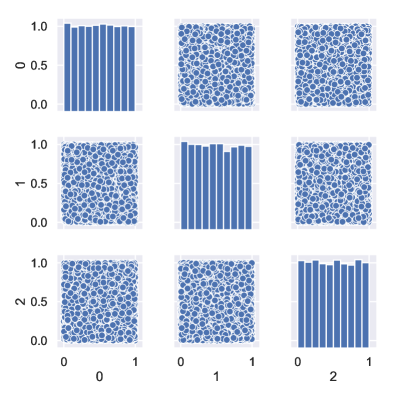
(b) Copula flow inverse $\boldsymbol{U}=\mathcal{C}_{\boldsymbol{U}_{\boldsymbol{X}}}^{-1}({\boldsymbol{U}_{\boldsymbol{X}}})$

Figure 5: The figure depicts inverse flow transformation of the 3 dimensional toy example in the Section 6. In the Figure 5a we can clearly see the copula structures in the off-diagonal scatter plots. The almost uniform distribution along the diagonal indicates that $\mathcal{F}_{\boldsymbol{X}}^{-1}\approx\boldsymbol{F}_{\boldsymbol{X}}$. The Figure 5b on the right shows inverse transform applied to the output of inverse flow, i.e. $\mathcal{C}_{\boldsymbol{X}}^{-1}\left(\mathcal{F}_{\boldsymbol{X}}^{-1}\approx\boldsymbol{F}_{\boldsymbol{C}X}\right)$. As the evident from scatter plots the copula flow and marginal flow together closely match true CDF see Appendix D.1

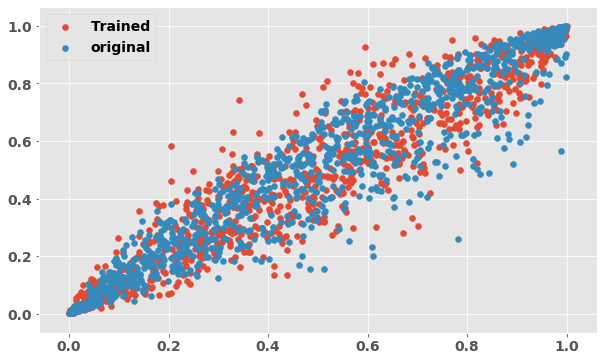
(a) Gumbel Copula

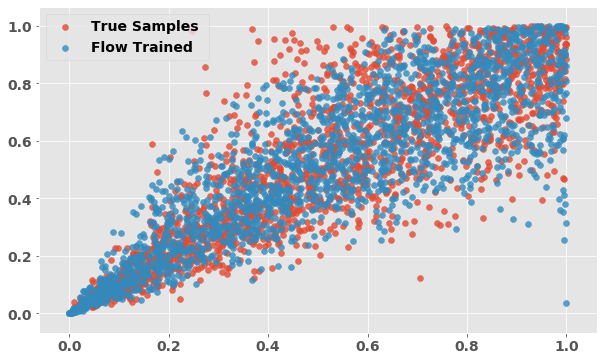
(b) Clayton Copula

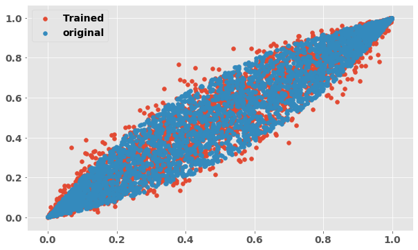
(c) Frank Copula

Figure 6: Learning bivariate Copulas using Copula Flow model. Each bi-variate density is learned by the same flow

Appendix C Definitions

Definition C.1

A distribution function (cumulative distribution function) is a function $F$ with domain $R=[-\infty,\infty]$, such that

• $F$ is non-decreasing

• $F(-\infty)$ = 0 and $F(\infty)=1$

• $F(x)=\mathrm{Pr}[X\leq x]\quad\forall x\in[-\infty,\infty]$

• $F$ is right continuous

Appendix D Universal Density Approximator

D.1 Copula Flows are Universal Density Approximators

Any invertible non-linear function that can take i.i.d. $\text{Uniform}\left[0,1\right]$ data and map it onto a density via monotone functions is a universal approximator [Hyvärinen and Pajunen, 1999].

The copula flow model can be used to represent any distribution function, i.e., the model is a universal density approximator. The inverse of the flow model can be interpreted as a CDF. By the probability integral transform and Theorem 1 in [Hyvärinen and Pajunen, 1999], we know that if $H_{X}$ is the CDF of the random variable then $H_{X}(X)$ is uniformly distributed in the hyper-cube $[0,1]^{d}$, where $d$ is the dimension of the vector.

In the following, we show that with the combination of marginal and copula flows we can learn any CDF with desired accuracy. Then the inverse of this CDF, i.e., the quantile function, can be used to generate random variables distributed according to $X$.

Convergence of the Marginal Flow

Proposition D.1

Monotonic rational quadratic splines can universally approximate any monotonic function with appropriate derivative approximations, see Theorem 3.1 in [Gregory and Delbourgo, 1982]

As discussed in section 2, a (quasi) inverse function $F^{-1}$ can be used to transform random variable $U\sim\text{Uniform}\left[0,1\right]$ to the random variable $X\sim F$. The inverse function is a monotonic function, and from Proposition D.1 we can say that

Lemma D.1

Given a flow map $\mathcal{F}_{X}:U\rightarrow\tilde{X}$, such that $\mathcal{F}_{X}$ converges point-wise to the true inverse function $F_{X}^{-1}$, the transformed random variable $\tilde{X}=\mathcal{F}_{X}(U)$ converges in distribution to the distribution $X=F_{X}^{-1}(U)$.

Proof: This is Portmanteau’s Theorem applied to flow functions based on Proposition D.1

Convergence of the Copula Flow

For any arbitrary ordering of the variables we have $\boldsymbol{U}=\boldsymbol{C}_{\boldsymbol{X}}(\boldsymbol{U}_{\boldsymbol{X}})$. We can write

$$U_{1} \doteq C_{X_{1}}(U_{X_{1}},\emptyset)=\mathrm{Pr}(U_{X_{1}}\leq u_{X_{1}}|\emptyset)\approx\mathcal{C}_{X_{1}}^{-1}(U_{X_{1}},\emptyset)$$ (21)

$$U_{k} \doteq C_{X_{k}}(U_{X_{k}},U_{X_{1:k-1}})$$ (22)

$$=\mathrm{Pr}(U_{X_{k}}\leq u_{X_{k}}|U_{X_{1:k-1}})$$ (23)

$$\approx\mathcal{C}_{X_{k}}^{-1}(U_{X_{k}},U_{X_{1:k-1}}),\qquad 2<k<d,$$ (24)

where $\emptyset$ indicates null set. According to [Hyvärinen and Pajunen, 1999], the variables $U_{1},\ldots,U_{d}$ are independently and uniformly distributed. The conditional copula flow is also modelled as a rational quadratic spline. From Lemma D.1 the $\mathcal{C}_{{\boldsymbol{X}}}^{-1}(\boldsymbol{U}_{\boldsymbol{X}})$ converges to the true copula CDF $\boldsymbol{C}_{\boldsymbol{X}}$. Therefore, $\boldsymbol{\mathcal{C}}_{\boldsymbol{X}}(\boldsymbol{U})$ converges in distribution to $\boldsymbol{U}_{X}$.

We can extend the conditional copula flow by adding the marginal flow $U_{X_{k}}=F_{X_{k}}(X_{k})$ to obtain

$$U_{k} \doteq C_{X_{k}}(F_{X_{k}}(X_{k}),F_{X_{1:k-1}}(X_{1:k-1}))=H_{X_{k}}(X_{k},X_{1:k-1})$$ (25)

$$=\mathrm{Pr}(X_{k}\leq x_{k}|X_{1:k-1})$$ (26)

$$\approx\mathcal{C}_{X_{k}}^{-1}(\mathcal{F}_{X_{k}}^{-1}(X_{k}),\mathcal{F}_{X_{1:k-1}}^{-1}(X_{1:k-1})),\qquad 2<k<d$$ (27)

From Theorem 1 in [Hyvärinen and Pajunen, 1999], the variables $U_{1},\ldots,U_{d}$ are independently and uniformly distributed. Moreover, the combined flow is monotonic as both the copula flow and marginal flow are monotonic. Hence, the inverse of the combined flow can transform any random vector $\boldsymbol{X}$ to uniform independent samples in the cube $\text{Uniform}\left[0,1\right]^{d}$.

The flows are learned as invertible monotonic functions. Therefore, using Lemma D.1 we obtain that the distribution $\mathcal{F}_{\boldsymbol{X}}^{-1}\left(\mathcal{C}_{\boldsymbol{X}}(\boldsymbol{U})\right)$ converges in distribution to $\boldsymbol{X}$. We can generate any random vector $\boldsymbol{X}$ starting from i.i.d. random variables. Hence, the copula flow model is universal density approximator.

Appendix E Software Details

A key point of our approach is the interpretation of normalising flow functions as a quantile function transforming a uniform density to the desired density via inverse transform sampling. As quantile functions are monotonic, we use monotone rational quadratic splines described in [Durkan et al., 2019] as a normalising flow function. However, we make changes to the original splines. These changes are necessary to ensure that the flow is learning quantile function.

• The univariate flow $\mathcal{F}$ maps from the $\text{Uniform}\left[0,1\right]$ to $\mathbf{ran}({F_{X}})$ of the random variable $X$. Hence, unlike [Durkan et al., 2019], our splines are asymmetric in their support.

• We modify the standard spline network to build a map as $(0,1)\rightarrow(B_{\text{lower}},B_{\text{upper}})$ where $B$ is the range of the marginal. Infinite support can be added with $B\to\infty$.

• We do not parametrise the knot positions by a neural network. We instead treat them as a free vector, i.e., $\boldsymbol{\theta}_{d}=[\boldsymbol{\theta}_{d}^{w},\boldsymbol{\theta}_{d}^{h},\boldsymbol{\theta}_{d}^{s}]$ are the width, height and slope parameters, respectively, that characterise the flow function for the independent marginals of data dimension $\mathcal{F}_{\boldsymbol{\theta}_{d}}$

• We map out-of-bound values back into the range and set the gradients of the flow map to $0$ at these locations.

For copula flow we use same network as autoregressive neural spline flows [Durkan et al., 2019]. As copula is a CDF defined over uniform densities, the copula flow spline maps $\text{Uniform}\left[0,1\right]\rightarrow\text{Uniform}\left[0,1\right]$. Apart from the change in the range of the splines, the copula flow architecture is sames as that of autoregressive neural spline flows [Durkan et al., 2019].

		Power	Gas	Hepmass	Miniboone	Synthetic Data
	Dimension	6	8	21	43	Various
	Train Data Points	1,615,917	852,174	315,123	29,556	Various
	Batch Size	2048	1024	1024	512	1024
Marginal Flow	Epochs	50	50	50	50	100
	Bins	512	512	512	512	512
	Learning Rate	1e-3	1e-3	1e-3	1e-3	1e-3
	Batch Size	512	512	512	512	512
Copula Flow	Epochs	100	100	100	50	100
	Bins	16	16	16	8	16
	Learning Rate	1e-4	1e-4	1e-4	1e-4	1e-4
	Hidden Features	[512, 512]	[256, 256]	[256, 256]	[128, 128]	[512, 512]
	Number of Flows	5	10	15	10	10

Table 4: Hyperprameters for the density estimation results

References

- Aas et al. [2009] K. Aas, C. Czado, A. Frigessi, and H. Bakken. Pair-Copula Constructions of Multiple Dependence. Insurance: Mathematics and Economics, 44(2):182–198, apr 2009. ISSN 01676687. doi: 10.1016/j.insmatheco.2007.02.001. URL http://www.sciencedirect.com/science/article/pii/S0167668707000194.
- Arjovsky and Bottou [2017] M. Arjovsky and L. Bottou. Towards Principled Methods for Training Generative Adversarial Networks. In International Conference on Learning Representations, ICLR, 2017. URL http://arxiv.org/abs/1701.04862.
- Beaulieu-Jones et al. [2019] B. K. Beaulieu-Jones, Z. S. Wu, C. Williams, R. Lee, S. P. Bhavnani, J. B. Byrd, and C. S. Greene. Privacy-Preserving Generative Deep Neural Networks Support Clinical Data Sharing. Circulation. Cardiovascular quality and outcomes, 2019. ISSN 19417705. doi: 10.1161/CIRCOUTCOMES.118.005122. URL https://www.ahajournals.org/doi/10.1161/CIRCOUTCOMES.118.005122http://www.ncbi.nlm.nih.gov/pubmed/31284738.
- Chang et al. [2019] B. Chang, S. Pan, and H. Joe. Vine Copula Structure Learning via Monte Carlo Tree Search. In Proceedings of Machine Learning Research, 2019. URL http://proceedings.mlr.press/v89/chang19a.html.
- Che et al. [2017] Z. Che, Y. Cheng, S. Zhai, Z. Sun, and Y. Liu. Boosting Deep Learning Risk Prediction with Generative Adversarial Networks for Electronic Health Records. In Proceedings - IEEE International Conference on Data Mining, ICDM, 2017. ISBN 9781538638347. doi: 10.1109/ICDM.2017.93. URL http://arxiv.org/abs/1709.01648.
- Choi et al. [2017] E. Choi, S. Biswal, B. Malin, J. Duke, W. F. Stewart, and J. Sun. Generating Multi-label Discrete Patient Records using Generative Adversarial Networks. In Machine Learning in Health Care (MLHC), mar 2017. URL http://arxiv.org/abs/1703.06490.
- Czado [2010] C. Czado. Pair-Copula Constructions of Multivariate Copulas BT - Copula Theory and Its Applications. In Copula Theory and Its Applications, volume 198, pages 93–109. Springer, 2010. ISBN 978-3-642-12465-5. doi: 10.1007/978-3-642-12465-5. URL https://www.jstor.org/stable/3663514http://www.springerlink.com/index/10.1007/978-3-642-12465-5{_}4{%}5Cnpapers2://publication/doi/10.1007/978-3-642-12465-5{_}4.
- David and Johnson [1948] F. N. David and N. L. Johnson. The probability integral transformation when parameters are estimated from the sample. Biometrika, 35(1/2):182–190, 1948. ISSN 00063444. URL http://www.jstor.org/stable/2332638.
- Dillon et al. [2017] J. V. Dillon, I. Langmore, D. Tran, E. Brevdo, S. Vasudevan, D. Moore, B. Patton, A. Alemi, M. Hoffman, and R. A. Saurous. TensorFlow Distributions. ArXiv Preprint, nov 2017. URL http://arxiv.org/abs/1711.10604.
- Dinh et al. [2015] L. Dinh, D. Krueger, and Y. Bengio. NICE: Non-linear Independent Components Estimation. In 3rd International Conference on Learning Representations, ICLR 2015 - Workshop Track Proceedings, 2015. URL http://arxiv.org/abs/1410.8516.
- Dinh et al. [2019] L. Dinh, J. Sohl-Dickstein, and S. Bengio. Density Estimation using Real NVP. In 5th International Conference on Learning Representations, ICLR, 2019. URL http://arxiv.org/abs/1605.08803.
- Durkan et al. [2019] C. Durkan, A. Bekasov, I. Murray, and G. Papamakarios. Neural Spline Flows. In Advances in Neural Information Processing Systems, Vancouver, 2019. URL http://arxiv.org/abs/1906.04032.
- Dwork and Roth [2013] C. Dwork and A. Roth. The Algorithmic Foundations of Differential Privacy. Foundations and Trends in Theoretical Computer Science, 2013. ISSN 15513068. doi: 10.1561/0400000042.
- Elidan [2010] G. Elidan. Copula Bayesian Networks. In Advances in Neural Information Processing Systems, 2010. URL http://papers.nips.cc/paper/3956-copula-bayesian-networks.
- Elliot and Domingo-Ferrer [2018] M. Elliot and J. Domingo-Ferrer. The Future of Statistical Disclosure Control. Technical report, Goverment Statistical Service, London, UK, dec 2018. URL http://arxiv.org/abs/1812.09204.
- Germain et al. [2015] M. Germain, K. Gregor, I. Murray, and H. Larochelle. MADE: Masked Autoencoder for Distribution Estimation. 32nd International Conference on Machine Learning, ICML, feb 2015. URL http://arxiv.org/abs/1502.03509.
- Goodfellow et al. [2014] I. J. Goodfellow, J. Pouget-Abadie, M. Mirza, B. Xu, D. Warde-Farley, S. Ozair, A. Courville, and Y. Bengio. Generative Adversarial Nets. In Advances in Neural Information Processing Systems, 2014. doi: 10.3156/jsoft.29.5_177_2. URL http://arxiv.org/abs/1406.2661.
- Gregory and Delbourgo [1982] J. A. Gregory and R. Delbourgo. Piecewise Rational Quadratic Interpolation to Monotonic Data. IMA Journal of Numerical Analysis, 2(2):123–130, apr 1982. ISSN 02724979. doi: 10.1093/imanum/2.2.123. URL https://academic.oup.com/imajna/article-lookup/doi/10.1093/imanum/2.2.123.
- Hansen [1994] B. E. Hansen. Autoregressive Conditional Density Estimation. International Economic Review, 35(3):705, aug 1994. ISSN 00206598. doi: 10.2307/2527081. URL https://www.jstor.org/stable/2527081?origin=crossref.
- Huang et al. [2018] C. W. Huang, D. Krueger, A. Lacoste, and A. Courville. Neural Autoregressive Flows. In 35th International Conference on Machine Learning, ICML, apr 2018. ISBN 9781510867963. URL http://arxiv.org/abs/1804.00779.
- Hyvärinen and Pajunen [1999] A. Hyvärinen and P. Pajunen. Nonlinear Independent Component Analysis: Existence and Uniqueness Results. Neural Networks, 12(3):429–439, apr 1999. ISSN 08936080. doi: 10.1016/S0893-6080(98)00140-3. URL https://www.sciencedirect.com/science/article/abs/pii/S0893608098001403.
- Joe [2005] H. Joe. Asymptotic Efficiency of the Two-stage Estimation Method for Copula-based Models. Journal of Multivariate Analysis, 94(2):401–419, jun 2005. ISSN 0047-259X. doi: 10.1016/J.JMVA.2004.06.003. URL https://www.sciencedirect.com/science/article/pii/S0047259X04001289.
- Jordon et al. [2019] J. Jordon, J. Yoon, and M. Van Der Schaar. PATE-GaN: Generating synthetic data with differential privacy guarantees. In 7th International Conference on Learning Representations, ICLR, 2019. URL https://www.semanticscholar.org/paper/PATE-GAN{%}3A-Generating-Synthetic-Data-with-Privacy-Jordon-Yoon/af1841e1db6579f1f1777a59c7e9e4658d2ac466.
- Kingma and Welling [2013] D. P. Kingma and M. Welling. Auto-Encoding Variational Bayes. arXiv preprint, 2013. URL http://arxiv.org/abs/1312.6114.
- Kingma et al. [2016] D. P. Kingma, T. Salimans, R. Jozefowicz, X. Chen, I. Sutskever, and M. Welling. Improved Variational Inference with Inverse Autoregressive Flow Diederik, jun 2016. URL https://arxiv.org/pdf/1606.04934.pdfhttp://arxiv.org/abs/1606.04934.
- Lopez-paz et al. [2013] D. Lopez-paz, J. M. Hernández-lobato, and Z. Ghahramani. Gaussian Process Vine Copulas for Multivariate Dependence. In 30th International Conference on Machine Learning, ICML, 2013. URL http://machinelearning.wustl.edu/mlpapers/papers/lopez-paz13.
- Müller et al. [2019] T. Müller, B. Mcwilliams, F. Rousselle, M. Gross, and J. Novák. Neural Importance Sampling. ACM Transactions on Graphics, 38(5):1–19, oct 2019. ISSN 07300301. doi: 10.1145/3341156. URL http://arxiv.org/abs/1808.03856http://arxiv.org/abs/1907.00503http://dl.acm.org/citation.cfm?doid=3341165.3341156.
- Nash and Durkan [2019] C. Nash and C. Durkan. Autoregressive Energy Machines. ArXiv Preprint, apr 2019. URL http://arxiv.org/abs/1904.05626.
- Nelsen [2006] R. B. Nelsen. An Introduction to Copulas. Springer New York, New York, NY, 2006. ISBN 978-0-387-28678-5. doi: 10.1007/0-387-28678-0_1. URL http://link.springer.com/10.1007/0-387-28678-0{_}1.
- Nikoloulopoulos and Karlis [2009] A. K. Nikoloulopoulos and D. Karlis. Modeling Multivariate Count Data Using Copulas. Communications in Statistics - Simulation and Computation, 39(1):172–187, dec 2009. ISSN 0361-0918. doi: 10.1080/03610910903391262. URL http://www.tandfonline.com/doi/abs/10.1080/03610910903391262.
- Oliva et al. [2018] J. B. Oliva, A. Dubey, M. Zaheer, B. Póczos, R. Salakhutdinov, E. P. Xing, and J. Schneider. Transformation Autoregressive Networks. In 35th International Conference on Machine Learning, ICML, volume 9, 2018. ISBN 9781510867963. URL http://arxiv.org/abs/1801.09819.
- Onken and Panzeri [2016] A. Onken and S. Panzeri. Mixed Vine Copulas as Joint Models of Spike Counts and Local Field Potentials. In Advances in Neural Information Processing Systems, 2016. URL http://papers.nips.cc/paper/6068-mixed-vine-copulas-as-joint-models-of-spike-counts-and-local-field-potentials.
- Papamakarios et al. [2017] G. Papamakarios, T. Pavlakou, and I. Murray. Masked Autoregressive Flow for Density Estimation. Advances in Neural Information Processing Systems, may 2017. ISSN 10495258. URL http://arxiv.org/abs/1705.07057.
- Papamakarios et al. [2019] G. Papamakarios, E. Nalisnick, D. J. Rezende, S. Mohamed, and B. Lakshminarayanan. Normalizing Flows for Probabilistic Modeling and Inference. ArXiv Preprint, dec 2019. URL https://arxiv.org/abs/1912.02762http://arxiv.org/abs/1912.02762.
- Park et al. [2018] N. Park, M. Mohammadi, K. Gorde, S. Jajodia, H. Park, and Y. Kim. Data Synthesis based on Generative Adversarial Networks. In Proceedings of the VLDB Endowment, jun 2018. doi: 10.14778/3231751.3231757. URL http://arxiv.org/abs/1806.03384http://dx.doi.org/10.14778/3231751.3231757.
- Patki et al. [2016] N. Patki, R. Wedge, and K. Veeramachaneni. The Synthetic Data Vault. In 3rd IEEE International Conference on Data Science and Advanced Analytics, DSAA, 2016. ISBN 9781509052066. doi: 10.1109/DSAA.2016.49.
- Rezende and Mohamed [2015] D. J. Rezende and S. Mohamed. Variational Inference with Normalizing Flows. In 32nd International Conference on Machine Learning, ICML, 2015. ISBN 9781510810587. URL https://arxiv.org/pdf/1505.05770.pdf.
- Rüschendorf [2009] L. Rüschendorf. On the Distributional Transform, Sklar’s Theorem, and the Empirical Copula Process. Journal of Statistical Planning and Inference, 2009. ISSN 03783758. doi: 10.1016/j.jspi.2009.05.030.
- Salimans et al. [2019] T. Salimans, A. Karpathy, X. Chen, and D. P. Kingma. PixelCNN++: Improving the PixelCNN with Discretized Logistic Mixture Likelihood and Other Modifications. In 5th International Conference on Learning Representations, ICLR, 2019. URL http://arxiv.org/abs/1701.05517.
- Sklar [1959] M. Sklar. Fonctions de Répartition à n Dimensions Et Leurs Marges. Publications of Institute Statistics University Paris (in French) 8, 1959. URL https://scholar.google.co.uk/scholar?hl=en{&}q={%}22Fonctions+de+r{{́e}}partition+{{̀a}}+n+dimensions+et+leurs+marges{%}22{&}btnG={&}as{_}sdt=1{%}2C5{&}as{_}sdtp={#}0.
- Srivastava et al. [2017] A. Srivastava, L. Valkov, C. Russell, M. U. Gutmann, and C. Sutton. VEEGAN: Reducing Mode Collapse in GANs using Implicit Variational Learning. In Advances in Neural Information Processing Systems, 2017.
- Tabak and Vanden-Eijnden [2010] E. G. Tabak and E. Vanden-Eijnden. Density Estimation by Dual Ascent of the Log-likelihood. Communications in Mathematical Sciences, 2010. ISSN 15396746. doi: 10.4310/CMS.2010.v8.n1.a11.
- Theis et al. [2016] L. Theis, A. Van Den Oord, and M. Bethge. A Note on the Evaluation of Generative Models. In 4th International Conference on Learning Representations, ICLR, 2016. URL http://arxiv.org/abs/1511.01844.
- Tran et al. [2019] D. Tran, K. Vafa, K. K. Agrawal, L. Dinh, and B. Poole. Discrete flows: Invertible Generative Models of Discrete ata. In Deep Generative Models for Highly Structured Data, DGS@ICLR 2019 Workshop, 2019. URL http://arxiv.org/abs/1905.10347.
- Wang et al. [2019] Z. Wang, Q. She, and T. E. Ward. Generative adversarial networks: A survey and taxonomy. arXiv preprint, 2019.
- Xu et al. [2019] L. Xu, M. Skoularidou, A. Cuesta-Infante, and K. Veeramachaneni. Modeling Tabular data using Conditional GAN. In Advances in Neural Information Processing Systems, jun 2019. URL http://arxiv.org/abs/1907.00503.
- Zhang et al. [2017] J. Zhang, G. Cormode, C. M. Procopiuc, D. Srivastava, and X. Xiao. Priv bayes: Private Data Release via Bayesian Networks. ACM Transactions on Database Systems, 2017. ISSN 15574644. doi: 10.1145/3134428.
- Ziegler and Rush [2019] Z. M. Ziegler and A. M. Rush. Latent Normalizing Flows for Discrete Sequences. In 36th International Conference on Machine Learning, ICML, 2019. ISBN 9781510886988. URL http://arxiv.org/abs/1901.10548.