Quantum mold casting for topological insulating and edge states

Abstract

We study the possibility of transferring fermions from a trivial system as particle source to an empty system but at topological phase as a mold for casting a stable topological insulator dynamically. We show that this can be realized by a non-Hermitian unidirectional hopping, which connects a central system at topological phase and a trivial flat-band system with a periodic driving chemical potential, which scans over the valence band of the central system. The near exceptional-point dynamics allows a unidirectional dynamical process: the time evolution from an initial state with full-filled source system to a stable topological insulating state approximately. The result is demonstrated numerically by a source-assistant QWZ model and SSH chain in the presence of random perturbation. Our finding reveals a classical analogy of quench dynamics in quantum matter and provides a way for topological quantum state engineering.

I Introduction

Preparing a topologically nontrivial state is of great interest for the task of quantum information processing. In general, a natural way for preparing a topological insulating state is cooling a system down to its ground state by suppressing the thermal fluctuations. An other intuitive way for preparation of topological insulating state is to follow a mechanical way by filling the topological energy band with fermions dynamically. However, it is tough to move fermions one by one from a particle source to an empty system since the fermion obeys the Schrodinger equation rather than the Newton’s laws. Recently, a dynamical way of realizing the topological phases by applying a time periodic global driving on a topologically trivial initial state is proposed. It has been shown that these periodic perturbations lead to the realization of new topological phases of matter which have no equilibrium counterparts TOKA ; TKIT ; MSRU ; LEFF ; HDEH ; JHWI , including topological insulators NHLI ; JCAY and edge states MTHA ; AKUN . It opens up a way to realize a topological phase dynamically. In these studies above, both the effective Hamiltonian dictating the non-equilibrium dynamics of the system and the initial static Hamiltonian are Hermitian. Nevertheless, a non-Hermitian Hamiltonian is no longer forbidden both in theory and experiment since the discovery that a certain class of non-Hermitian Hamiltonians could exhibit entirely real spectra Bender ; Bender1 . The origin of the reality of the spectrum of a non-Hermitian Hamiltonian is the pseudo-Hermiticity of the Hamiltonian operator Ali1 . It motives a non-Hermitian extension of the dynamical preparation of a topologically nontrivial state. In addition, the peculiar features of a non-Hermitian system do not only manifest in statics but also dynamics. Non-Hermitian systems exhibit many peculiar dynamic behaviors that never occurred in Hermitian systems. One of the remarkable features is the dynamics at exceptional point (EP) HeissEP ; RotterEPJPA ; HXu or spectral singularity (SS) AMprl ; SLHprb ; AAA ; BFS ; ZXZ2 , where the system has a coalescence state. Exclusively, EP dynamics has recently emerged as transformative tools for dynamically evolving quantum systems into a quantum phase with desirable properties XZZH ; XZZHarxiv ; XMYA . It is expected that the introduction of non-Hermitian elements benefits to the scheme for quantum state engineering.

In this work, we focus on the EP-related dynamic behavior for the many-body system. From the perspective of non-Hermitian quantum mechanics, it is also a challenge to deal with many-particle dynamics. As an application, we study the possibility of transferring fermions from a trivial system as particle source to an empty system but at topological phase as a mold for casting a stable topological insulator dynamically. We show that this can be realized by a non-Hermitian connection between a central system at topological phase and a flat-band system with a periodic driving chemical potential. After sufficient long time, the near exceptional-point dynamics allows the time evolution from an initial state with full-filled source system to a stable topological insulating state approximately. We demonstrate the scheme by numerical simulations for a source-assistant QWZ model and SSH chain in the presence of random perturbation. The result reveals a classical analogy of quench dynamics in quantum matter and provides a way for topological quantum state engineering. It also shows that a unidirectional tunneling supports an exclusive feature never occurs in Hermitian system, which can be utilized to quantum state engineering. Our findings pave the way for establishing EP-dynamics based techniques as a powerful and versatile tool for topological state engineering.

This paper is organized as follows. In Section II, we describe the model Hamiltonian and give the condition for the existence of coalescing state. In Section III, based on the solutions, we present the characteristics of the EP dynamics in a source-assistant QWZ model and the details of dynamical formation of topological insulating state. In Section IV, we propose a dynamical way to cast edge states in a source-assistant RM model. Finally, we give a summary and discussion in Section V.

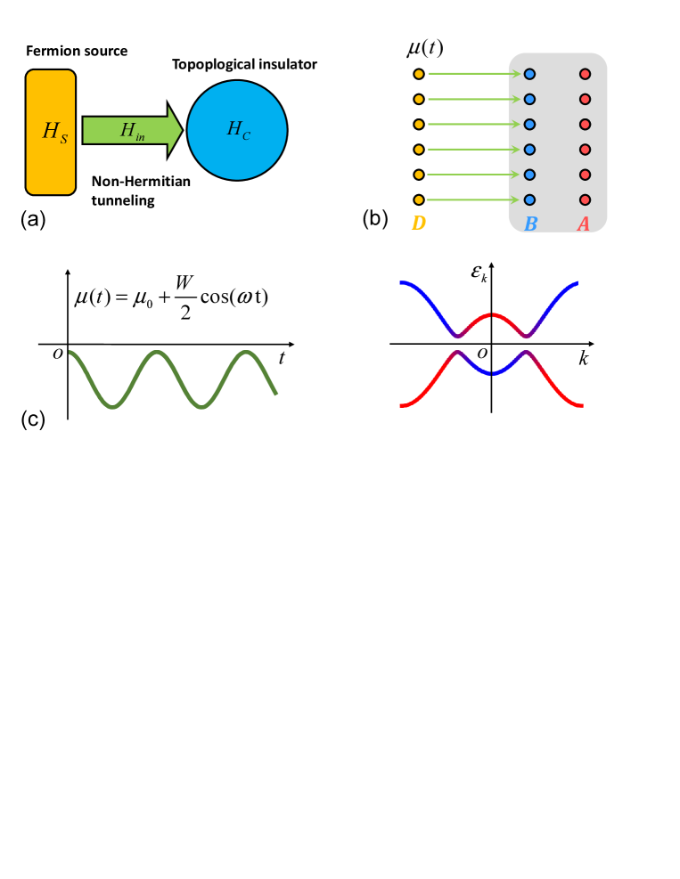
Figure 1: Schematics for the system and process of quantum mold casting. (a) The system consists of two parts, central system $H_{\mathrm{c}}$ and source system $H_{\mathrm{s}}$. The target state is the ground state of $H_{\mathrm{c}}$, which can be topologically non-trivial or not. $H_{\mathrm{s}}$ is a topologically trivial system, providing the supply of fermions. Both $H_{\mathrm{c}}$ and $H_{\mathrm{s}}$ are Hermitian, while $H_{\mathrm{in}}$ is non-Hermitian, representing the connection between $H_{\mathrm{c}}$ and $H_{\mathrm{s}}$, and taking the role to transport fermions unidirectionally from $H_{\mathrm{s}}$ to $H_{\mathrm{c}}$. (b) A tight-binding model for the scheme, which contains three sets, A, B, and D. Lattices A and B (red and blue filled circles) embedded in the shadow area is topological insulator, while lattice D (yellow filled circle) is a flat-band (hopping-free) system but with oscillating chemical potential. Green arrows represent unidirectional hopping from D to B lattices. The aim of this work is to realize the following process via time evolution. Initially, D lattice is fully filled, while A and B are empty. The final state is expected to a half-filled ground state of $H_{\mathrm{c}}$. (c) The underlying mechanism of the dynamic process. At instant $t_{\mathbf{k}}$, the chemical potential and energy levels of $H_{\mathrm{c}}$ are resonant, leading to exceptional points. The corresponding (EP) dynamics allows a complete transfer of fermions between the degenerate energy levels. In the long-time limit, such dynamics occurs at each $\mathbf{k}$ sector again and again. It is expected the lower band of $H_{\mathrm{c}}$ can be completely filled.

II Model and coalescing state

We consider a non-Hermitian time-dependent Hamiltonian

$$H=H_{\mathrm{c}}+H_{\mathrm{s}}+H_{\mathrm{in}},$$ (1)

with

$$H_{\mathrm{c}}=\sum_{i,j=1}^{N}\left(T_{ij}a_{i}^{{\dagger}}b_{j}+A_{ij}a_{i}^{{\dagger}}a_{j}+B_{ij}b_{i}^{{\dagger}}b_{j}+\mathrm{H.c.}\right),$$ (2)

and

$$H_{\mathrm{s}}=\mu(t)\sum_{j=1}^{N}d_{j}^{{\dagger}}d_{j}\text{, }H_{\mathrm{in}}=\gamma\sum_{j=1}^{N}b_{j}^{{\dagger}}d_{j},$$ (3)

where $a_{j}$, $b_{j}$, and $d_{j}$ are fermion operators and $\mu(t)=\mu_{0}+\frac{W}{2}\cos(\omega t)$ is periodic driving chemical potential, with parameters $\left\{T_{ij},A_{ij},B_{ij}\right\}$ depending on $H_{\mathrm{c}}$ ($\mu_{0}$ is an average of the negative energy levels and $W$ is the bandwidth of $H_{\mathrm{c}}$). Here both $H_{\mathrm{c}}$ and $H_{\mathrm{s}}$ are Hermitian, describing the central system and source system, respectively. Notably, $H_{\mathrm{in}}$ is a non-Hermitian term, representing the connection between two systems $H_{\mathrm{c}}$ and $H_{\mathrm{s}}$.

For a central system with the periodic boundary condition, after performing Fourier transformation, we have $H=\sum_{\mathbf{k}}H_{\mathbf{k}}$, where the sub-Hamiltonian $H_{\mathbf{k}}$ in each invariant sub-space can be expressed as

$$H_{\mathbf{k}}=\left(\begin{array}[]{ccc}a_{\mathbf{k}}^{{\dagger}}&b_{\mathbf{k}}^{{\dagger}}&d_{\mathbf{k}}^{{\dagger}}\end{array}\right)h_{\mathbf{k}}\left(\begin{array}[]{c}a_{\mathbf{k}}\\ b_{\mathbf{k}}\\ d_{\mathbf{k}}\end{array}\right),$$ (4)

where

$$\left(\begin{array}[]{ccc}a_{\mathbf{k}}^{{\dagger}}&b_{\mathbf{k}}^{{\dagger}}&d_{\mathbf{k}}^{{\dagger}}\end{array}\right)=\sum_{\mathbf{r}}\frac{e^{i\mathbf{k\cdot r}}}{\sqrt{N}}\left(\begin{array}[]{ccc}a_{\mathbf{r}}^{{\dagger}}&b_{\mathbf{r}}^{{\dagger}}&d_{\mathbf{r}}^{{\dagger}}\end{array}\right).$$ (5)

In general, the Bloch matrix $h_{\mathbf{k}}$ has the form

$$h_{\mathbf{k}}=\left(\begin{array}[]{ccc}B_{z}(\mathbf{k)}&B_{x}(\mathbf{k)}-iB_{y}(\mathbf{k)}&0\\ B_{x}(\mathbf{k)}+iB_{y}(\mathbf{k)}&-B_{z}(\mathbf{k)}&\gamma\\ 0&0&\mu(t)\end{array}\right),$$ (6)

where a term related to the identity matrix $I_{3}$ is neglected. Here, vector $\mathbf{B}(\mathbf{k)}$ is obtained by the set of parameters $\left\{T_{ij},A_{ij},B_{ij}\right\}$. We note that the time-dependent $\mu(t)$ does not break the translational symmetry (also other all symmetries), allowing the exact diagonalization of $H$ via that of each $3\times 3$ matrix. Accordingly, the time evolution can also be computed via the complete set of $3\times 3$ matrices.

Here we focus on two points of particular interest: i) We note that in $k$ space, the central Hamiltonian can be expressed as

$$H_{\mathrm{c}}=\sum_{\mathbf{k}}\left(\begin{array}[]{cc}a_{\mathbf{k}}^{{\dagger}}&b_{\mathbf{k}}^{{\dagger}}\end{array}\right)\mathbf{B}_{\mathbf{k}}\cdot\mathbf{\sigma}\left(\begin{array}[]{c}a_{\mathbf{k}}\\ b_{\mathbf{k}}\end{array}\right),$$ (7)

by Pauli matrices $\mathbf{\sigma}$, and then can be topologically non-trivial or not, depending on the explicit form of $\mathbf{B}_{\mathbf{k}}$. ii) For a given $\mathbf{k}$, matrix $h_{\mathbf{k}}$ contains a Jordan block at instant $t=t_{\mathbf{k}}$, where $t_{\mathbf{k}}$ satisfies the equation

$$\mu(t_{\mathbf{k}})=\pm\left|\mathbf{B}(\mathbf{k)}\right|.$$ (8)

In this case, there are only two eigenstates for $h_{\mathbf{k}}$, which are the eigenstates of $\mathbf{B}_{\mathbf{k}}\cdot\mathbf{\sigma}$, and then the completeness of eigenstates is spoiled.

Actually, in general, matrix $h_{\mathbf{k}}$ can be rewritten as

$$h_{\mathbf{k}}=\left|B(\mathbf{k)}\right|\left(\begin{array}[]{ccc}\cos\theta_{\mathbf{k}}&\sin\theta_{\mathbf{k}}e^{-i\varphi_{\mathbf{k}}}&0\\ \sin\theta_{\mathbf{k}}e^{i\varphi_{\mathbf{k}}}&-\cos\theta_{\mathbf{k}}&\gamma_{\mathbf{k}}\\ 0&0&\Delta_{\mathbf{k}}\end{array}\right),$$ (9)

where parameters in the matrix elements are defined as

$$\tan\theta_{\mathbf{k}} = \frac{B_{z}(\mathbf{k)}}{\left|B(\mathbf{k)}\right|},\tan\varphi_{\mathbf{k}}=\frac{B_{x}(\mathbf{k)}}{B_{y}(\mathbf{k)}},$$

$$\gamma_{\mathbf{k}} = \gamma/\varepsilon_{\mathbf{k}},\Delta_{\mathbf{k}}=\mu/\varepsilon_{\mathbf{k}},\varepsilon_{\mathbf{k}}=\left|B(\mathbf{k)}\right|.$$ (10)

Note that although matrix $h_{\mathbf{k}}$ is non-Hermitian, its eigenvalues are always real. Three eigenvectors are obtained as

$$\left|\psi_{\mathbf{k}}^{+}\right\rangle = \left(\begin{array}[]{c}\cos\frac{\theta_{k}}{2}\\ e^{i\varphi_{k}}\sin\frac{\theta_{k}}{2}\\ 0\end{array}\right),\left|\psi_{\mathbf{k}}^{\mathbf{-}}\right\rangle=\left(\begin{array}[]{c}-\sin\frac{\theta_{k}}{2}\\ e^{i\varphi_{k}}\cos\frac{\theta_{k}}{2}\\ 0\end{array}\right),$$ (17)

$$\left|\psi_{\mathbf{k}}^{\Delta}\right\rangle = \left(\begin{array}[]{c}\gamma_{k}e^{-i\varphi_{k}}\sin\theta_{k}\\ \gamma_{k}\left(\Delta_{k}-\cos\theta_{k}\right)\\ \Delta_{k}^{2}-1\end{array}\right),$$ (21)

with the eigenvalues

$$\varepsilon_{\mathbf{k}}^{\pm}=\pm\varepsilon_{\mathbf{k}},\varepsilon_{\mathbf{k}}^{\Delta}=\Delta_{k}\varepsilon_{\mathbf{k}}.$$ (22)

It shows that when taking $\Delta_{\mathbf{k}}=\pm 1$, or at $t=t_{\mathbf{k}}$, matrix $h_{\mathbf{k}}$ reaches at the EP. And we have $\left|\psi_{\mathbf{k}}^{\Delta}\right\rangle=\left|\psi_{\mathbf{k}}^{\pm}\right\rangle$, i.e., the coalescing state appears, which is crucial for the scheme in this work.

III EP dynamics and periodic driving

Based on the above analysis, the dynamics of $H$ is governed by the time evolution operator

$$U(t)=\exp(-iHt)=\prod_{\mathbf{k}}U_{\mathbf{k}}(t),$$ (23)

where the time evolution operator in sub-space $\mathbf{k}$ has the form

$$U_{\mathbf{k}}(t)=\mathcal{T}\exp[-i\int_{0}^{t}H_{\mathbf{k}}(t^{\prime})\text{{d}}t^{\prime}],$$ (24)

with $\mathcal{T}$ being the time-order operator. We first consider the case with slowly varying $H_{\mathbf{k}}(t)$ (i.e., very small $\omega$). The time evolution around the instant $t=t_{\mathbf{k}}$ is crucial and can be described approximately by the operator

$$U_{\mathbf{k}}(t)\approx\exp[-iH_{\mathbf{k}}(t_{\mathbf{k}})t],$$ (25)

which obeys an exclusive EP dynamics.

Considering a time-independent $h_{\mathbf{k}}^{\mathrm{EP}}$ at EP,

$$h_{\mathbf{k}}^{\mathrm{EP}}=\varepsilon_{\mathbf{k}}\left(\begin{array}[]{ccc}\cos\theta_{\mathbf{k}}&\sin\theta_{\mathbf{k}}e^{-i\varphi_{\mathbf{k}}}&0\\ \sin\theta_{\mathbf{k}}e^{i\varphi_{\mathbf{k}}}&-\cos\theta_{\mathbf{k}}&\gamma_{\mathbf{k}}\\ 0&0&-1\end{array}\right),$$ (26)

which contains a Jordan block, satisfying

$$h_{\mathbf{k}}^{\mathrm{EP}}\left|\psi_{\mathbf{k}}^{\pm}\right\rangle=\pm\varepsilon_{\mathbf{k}}\left|\psi_{\mathbf{k}}^{\pm}\right\rangle,h_{\mathbf{k}}^{\mathrm{EP}}\left|\psi_{\mathbf{k}}^{\mathrm{a}}\right\rangle=-\varepsilon_{\mathbf{k}}\left|\psi_{\mathbf{k}}^{\mathrm{a}}\right\rangle.$$ (27)

Here vector

$$\left|\psi_{\mathbf{k}}^{\mathrm{a}}\right\rangle=\left(0,0,1\right)^{\mathrm{T}}$$ (28)

is referred to as auxiliary vector, while $\left|\psi_{\mathbf{k}}^{-}\right\rangle$ is the coalescing state.

Straightforward derivation shows that

$$\exp\left(-ih_{\mathbf{k}}^{\mathrm{EP}}t\right)=-\frac{\gamma_{k}\varepsilon_{\mathbf{k}}t}{2}$$

$$\times[\sin\left(\varepsilon_{\mathbf{k}}t\right)+i(1+2\sin^{2}\frac{\varepsilon_{\mathbf{k}}t}{2})]A$$

$$+\cos\left(\varepsilon_{\mathbf{k}}t\right)I_{3}-i\sin\left(\varepsilon_{\mathbf{k}}t\right)\left(\frac{h_{\mathbf{k}}^{\mathrm{EP}}}{\varepsilon_{\mathbf{k}}}+\frac{\gamma_{k}A}{2}\right),$$ (29)

where the matrix

$$A=\left(\frac{h_{\mathbf{k}}^{\mathrm{EP}}}{\varepsilon_{\mathbf{k}}}\right)^{2}-I_{3}=\left(\begin{array}[]{ccc}0&0&-\sin\frac{\theta_{k}}{2}\\ 0&0&e^{i\varphi_{k}}\cos\frac{\theta_{k}}{2}\\ 0&0&0\end{array}\right),$$ (30)

satisfying

$$A\left|\psi_{\mathbf{k}}^{\mathrm{a}}\right\rangle=\left|\psi_{\mathbf{k}}^{-}\right\rangle.$$ (31)

The time evolution operator contains terms with linear and periodic functions of $t$. Then the time evolution for initial state $\left|\psi_{\mathbf{k}}^{\mathrm{a}}\right\rangle$ is

$$\left|\psi_{\mathbf{k}}^{\mathrm{EP}}\left(t\right)\right\rangle=\exp\left(-ih_{\mathbf{k}}^{\mathrm{EP}}t\right)\left|\psi_{\mathbf{k}}^{\mathrm{a}}\right\rangle$$ (32)

$$= -\frac{\gamma_{k}\varepsilon_{\mathbf{k}}t}{2}\times[\sin\left(\varepsilon_{\mathbf{k}}t\right)+i(1+2\sin^{2}\frac{\varepsilon_{\mathbf{k}}t}{2})]\left|\psi_{\mathbf{k}}^{-}\right\rangle$$

$$+\cos\left(\varepsilon_{\mathbf{k}}t\right)\left|\psi_{\mathbf{k}}^{\mathrm{a}}\right\rangle-i\sin\left(\varepsilon_{\mathbf{k}}t\right)\left(\frac{\gamma_{k}}{2}-1\right)\left|\psi_{\mathbf{k}}^{-}\right\rangle.$$

It indicates that the long-time evolution of initial state $d_{\mathbf{k}}^{{\dagger}}\left|0\right\rangle_{\mathbf{k}}$ ($\left|0\right\rangle_{\mathbf{k}}$ is the vacuum state for operators $a_{\mathbf{k}}$, $b_{\mathbf{k}}$, and $d_{\mathbf{k}}$.) turns to the coalescing state $\left|\psi_{\mathbf{k}}^{-}\right\rangle$ due to the linear-time dependence of the first term. Obviously, the action of $U_{\mathbf{k}}(t)$ at long time is the projection of any pure initial state on the component $\left|\psi_{\mathbf{k}}^{-}\right\rangle$, which is perfect transport of fermion from the source to the central system. For many-particle case, we note that all the time-dependent $h_{\mathbf{k}}$ can not reach their $h_{k}^{\mathrm{EP}}$, simultaneously. The dynamics for $h_{k}$ near EP may result in the oscillation of the particle number between the source and the central systems, although the hopping term is unidirectional. Nevertheless, periodically varying $\mu(t)$ passes by the EP of every $h_{\mathbf{k}}$ is expected to transport the fermion from source to the central system in each $\mathbf{k}$ sector near completely. Ideally, if this occurs in every $\mathbf{k}$ sector, the full-filled initial state

$$\prod_{j}d_{j}^{{\dagger}}\left|0\right\rangle=\prod_{\mathbf{k}}d_{\mathbf{k}}^{{\dagger}}\left|0\right\rangle$$ (33)

will evolve to the ground state of the central system meanwhile leaving empty in the source system. Note that the initial state is a trivial many-particle state, a saturatedly filled state. The aim of the scheme is to prepare a nontrivial state from such an initial state through the time evolution in the context of non-Hermitian quantum mechanics.

To illustrate our scheme and investigate its efficiency, we consider the central system as QWZ model introduced by Qi, Wu and Zhang QWZ . The Bloch Hamiltonian is

$$h_{\mathbf{k}}=B_{x}\sigma_{x}+B_{y}\sigma_{y}+B_{z}\sigma_{z},$$ (34)

where the field components are

$$B_{x} = \sin k_{x},B_{y}=\sin k_{y},$$

$$B_{z} = u+\cos k_{x}+\cos k_{y}.$$ (35)

It is well known that the Chern number of the lower band is

$$c = 0,\text{for }\left|u\right|>2,$$

$$c = \pm 1,\text{for }0<\pm u<2.$$ (36)

Numerical simulation is performed to verify the efficiency of the scheme. Here the computation for time-ordered integral is performed by using a uniform mesh in the time discretization for the time-dependent Hamiltonian $h_{\mathbf{k}}(t)$ with deferent $\omega$. We compute the time evolution for the initial state $\left|\psi_{\mathbf{k}}\left(0\right)\right\rangle=d_{\mathbf{k}}^{{\dagger}}\left|0\right\rangle_{\mathbf{k}}$, and compare the evolved state $\left|\psi_{\mathbf{k}}\left(t\right)\right\rangle$ with the target state

$$\left|\psi_{\mathbf{k}}^{\text{c}}\right\rangle=\left(\sin\frac{\theta_{k}}{2}a_{\mathbf{k}}^{{\dagger}}-e^{i\varphi_{k}}\cos\frac{\theta_{k}}{2}b_{\mathbf{k}}^{{\dagger}}\right)\left|0\right\rangle_{\mathbf{k}},$$ (37)

which is the coalescing state of $h_{\mathbf{k}}$ [Eq. (34)] at EP with negative energy. The observables are particle number left in the source system

$$n\left(t\right)=\frac{1}{N}\sum_{\mathbf{k}}\frac{\left\langle\psi_{\mathbf{k}}\left(t\right)\right|d_{\mathbf{k}}^{{\dagger}}d_{\mathbf{k}}\left|\psi_{\mathbf{k}}\left(t\right)\right\rangle}{\left|\left|\psi_{\mathbf{k}}\left(t\right)\right\rangle\right|^{2}},$$ (38)

and the fidelity

$$F\left(t\right)=\frac{1}{N}\sum_{\mathbf{k}}\frac{\left|\langle\psi_{\mathbf{k}}^{\text{c}}\left|\psi_{\mathbf{k}}\left(t\right)\right\rangle\right|}{\left|\left|\psi_{\mathbf{k}}^{\text{c}}\right\rangle\left|\psi_{\mathbf{k}}\left(t\right)\right\rangle\right|},$$ (39)

which measure the efficiency of the transport. The numerical results for finite systems with presentative parameters are plotted in Fig. 2. We see that the optimal efficiency occurs when $\omega=0.001$, and the transport efficiency decreases gradually with the increasing of $\omega.$

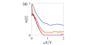
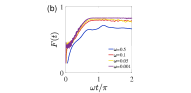
Figure 2: Plots of $n\left(t\right)$ and $F\left(t\right)$, which are defined in Eqs. (38) and Eq. (39), obtained by exact diagonalization for finite system. The parameters are $N=20\times 20$, $u=1.2$, $\mu_{0}=-2$, $W=2.6$, and $\gamma=0.5$. Four typical values of $\omega$ are taken, and indicated in the panels.

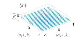
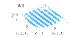
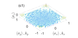
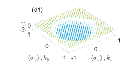
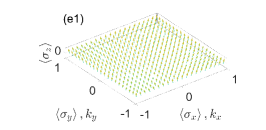
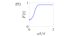
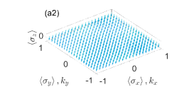
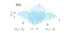
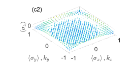
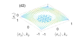
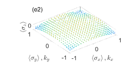
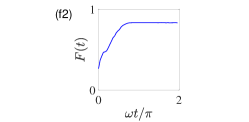
Figure 3: Plots of skyrmion pattern at several typical instants, which are defined in Eq. (41), obtained by exact diagonalization for finite system. The corresponding fidelity is also plotted as comparison. The parameters are $N=20\times 20$, $\omega=0.001$, $\gamma=0.5$, (a1)-(d1) $u=3.2$, $\mu_{0}=-3.21$, $W=3.94$, and (a2)-(d2) $u=1.2$, $\mu_{0}=-2$, $W=2.38$, which correspond to the central systems in topologically trivial and non-trivial phases, respectively.

We also compute the time-dependent skyrmion to characterize the formation process of the target state. To this end we introduce the auxiliary matrices

$$\Sigma_{\alpha}=\left(\begin{array}[]{cc}\sigma_{\alpha}&0\\ 0&1\end{array}\right),\Sigma_{0}=\left(\begin{array}[]{cc}I_{2}&0\\ 0&1\end{array}\right),$$ (40)

where $\sigma_{\alpha}$ is Pauli matrix in $\alpha$ ($\alpha=x,y,z$) component and $I_{2}$ is unit matrix. The time-dependent skyrmion is evaluated as

$$\left\langle\sigma_{\alpha}\right\rangle_{\mathbf{k},t}=\frac{\left\langle\psi_{\mathbf{k}}\left(t\right)\right|\Sigma_{\alpha}\left|\psi_{\mathbf{k}}\left(t\right)\right\rangle}{\left\langle\psi_{\mathbf{k}}\left(t\right)\right|\Sigma_{0}\left|\psi_{\mathbf{k}}\left(t\right)\right\rangle}.$$ (41)

Unlike the expectation value of Pauli matrix $\sigma_{\alpha}$ in the usual study LS PRA , $\left\langle\sigma_{\alpha}\right\rangle_{\mathbf{k},0}=0$ for all $\alpha$ and $\sum_{\alpha=x,y,z}\left(\left\langle\sigma_{\alpha}\right\rangle_{\mathbf{k},t}\right)^{2}\leqslant 1$. In the case that all the fermions have been transported to the central system in long-time limit the skyrmion obeys the pattern

$$\left\langle\mathbf{\sigma}\right\rangle_{\mathbf{k},\infty}=\frac{\mathbf{B}(\mathbf{k)}}{\left|\mathbf{B}(\mathbf{k)}\right|},$$ (42)

which characterizes the topological feature of the phase. The numerical results for finite systems with presentative parameters, $\left\langle\sigma_{\alpha}\right\rangle_{\mathbf{k},t}$ at different time are plotted in Fig. 3. Fig. 3 (e1) and (e2) clearly show that in long-time limit the skyrmion exhibits approximately the pattern defined in Eq. (42), which correspond to the central systems in topologically trivial and non-trivial phases, respectively.

IV Edge states engineering

The aforementioned formalism is developed in the system with translational symmetry in order to simplify the calculation procedure. This section will be devoted to the realization of quantum mold casting in a system without the translational symmetry. The essential step for this extension is replacing the index $\mathbf{k}$ by the eigenmodes of $H_{\mathrm{c}}$. Two facts, flat band of $H_{\mathrm{s}}$ and uniform hopping in $H_{\mathrm{in}}$, still allow $H$ to be block diagonalizable.

To demonstrate this point, we consider the central system $H_{\mathrm{c}}$ to be a generalized RM chain with the Hamiltonian

$$H_{\mathrm{c}} = \sum_{j=1}^{N-1}\left(w_{j}a_{j}^{{\dagger}}b_{j}+v_{j}a_{j+1}^{{\dagger}}b_{j}+\mathrm{H.c.}\right)$$ (43)

$$+V\sum_{j=1}^{N}\left(a_{j}^{{\dagger}}a_{j}-b_{j}^{{\dagger}}b_{j}\right),$$

where $w_{j}$ and $v_{j}$ are position dependent hopping amplitudes (including random distributions). The other Hamiltonians has a slight change from the original form

$$H_{\mathrm{s}}=\mu(t)\sum_{j=1}^{N}d_{j}^{{\dagger}}d_{j}\text{, }H_{\mathrm{in}}=\gamma\sum_{j=1}^{N}\left(a_{j}^{{\dagger}}d_{j}+b_{j}^{{\dagger}}d_{j}\right).$$ (44)

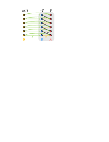
Figure 4: schematic of the system with a generalized RM chain as the central system $H_{\text{c}}$. Each part of the system is represented by Eq.(43) and Eq.(44), respectively.

A schematics of the system is presented in Fig. 4. The Hamiltonian $H_{\mathrm{c}}$ can be written as the diagonal-block form

$$H = \sum_{n=1}^{N}H_{n},$$ (45)

$$H_{n} = \left(\begin{array}[]{ccc}f_{a,n}^{{\dagger}}&f_{b,n}^{{\dagger}}&f_{d,n}^{{\dagger}}\end{array}\right)h_{n}\left(\begin{array}[]{c}f_{a,n}\\ f_{b,n}\\ f_{d,n}\end{array}\right),$$ (50)

which reduces the eigenproblem of the present $H$ to that of $3\times 3$ matrix. Here the Bloch-like matrix $h_{n}$ has the form

$$h_{n}=\left(\begin{array}[]{ccc}V&\varepsilon_{0}(n)&\gamma\\ \varepsilon_{0}(n)&-V&\gamma\\ 0&0&\mu(t)\end{array}\right),$$ (51)

and three sets of canonical fermion operators are defined as

$$f_{a,n}^{{\dagger}} = \sum_{j=1}^{N}A_{j}^{n}a_{j}^{{\dagger}},\text{ }f_{b,n}^{{\dagger}}=\sum_{j=1}^{N}B_{j}^{n}b_{j}^{{\dagger}},$$

$$f_{d,n}^{{\dagger}} = \sum_{j=1}^{N}B_{j}^{n}d_{j}^{{\dagger}}.$$ (52)

with real coefficients $A_{j}^{n}$ and $B_{j}^{n}\$being obtained by single-particle eigenstates of $H_{\mathrm{c}}$ at $V=0$, with eigenvalues $\pm\varepsilon_{0}(n)$, satisfying the orthonormal complete relations

$$\sum_{j}\left(A_{j}^{m}\right)^{\ast}A_{j}^{n} = \sum_{j}\left(B_{j}^{m}\right)^{\ast}B_{j}^{n}=\delta_{mn},$$

$$\sum_{n}\left(A_{i}^{n}\right)^{\ast}A_{j}^{n} = \sum_{n}\left(B_{i}^{n}\right)^{\ast}B_{j}^{n}=\delta_{ij},$$ (53)

Actually, the Hamiltonian of SSH chain is diagonalized as

$$H_{\mathrm{c}}\left(V=0\right)=\sum_{n=1}^{N}\varepsilon_{0}(n)(f_{+,n}^{{\dagger}}f_{+,n}-f_{-,n}^{{\dagger}}f_{-,n}),$$ (54)

where $\varepsilon_{0}(n)>0$ is the positive energy spectrum with $n\in[1,N]$, and

$$f_{\pm,n}^{{\dagger}}=\frac{1}{\sqrt{2}}\left(f_{a,n}^{{\dagger}}\pm f_{b,n}^{{\dagger}}\right),$$ (55)

due to the fact that SSH chain is a bipartite lattice. We note that $h_{n}$ is essentially the counterpart of $h_{\mathbf{k}}$ in the Eq. (9) with a slight difference. The time evolution driven by $h_{n}$ is similar to that of $h_{\mathbf{k}}$, including the EP dynamics.

The central system $H_{\mathrm{c}}$ is the simplest prototype of a topologically nontrivial band insulator with a symmetry protected topological phase Ryu ; Wen . In recent years, it has been attracted much attention and extensive studies have been demonstrated XD ; Hasan ; Delplace ; ChenS1 ; ChenS2 ; LS PRA ; WRPRA ; WRPRB . In the uniform case, $w=w_{j}<v=v_{j}$, there are two edge sates with eigenvalues $\pm V$, for large $N$, which are explicitly expressed as

$$\left|\text{L}\right\rangle = \Omega\sum\limits_{j=1}^{N}\left(-\frac{w}{v}\right)^{j-1}a_{j}^{\dagger}\left|0\right\rangle,$$ (56)

$$\left|\text{R}\right\rangle = \Omega\sum\limits_{j=1}^{N}\left(-\frac{w}{v}\right)^{N-j}b_{j}^{\dagger}\left|0\right\rangle,$$ (57)

where the normalization factor is $\Omega=\sqrt{1-\left(\frac{w}{v}\right)^{2}}$. In addition, small random perturbations on $w$ and $v$ cannot remove the edge states and change their eigenvalues. Taking suitable value of $V$, two edge states can lie within the gap of the spectrum. In the following, we perform numerical simulation of time evolution for the full-filled initial state

$$\left|\psi\left(0\right)\right\rangle=\prod_{j}d_{j}^{{\dagger}}\left|0\right\rangle=\prod_{n}d_{n}^{{\dagger}}\left|0\right\rangle,$$ (58)

by taking several different values of $\omega$ in $\mu(t)$. The evolved state obeys

$$\left|\psi\left(t\right)\right\rangle=\prod_{n}\left|\psi_{n}\left(t\right)\right\rangle=U(t)\prod_{n}d_{n}^{{\dagger}}\left|0\right\rangle,$$ (59)

where the time evolution operator has the similar form as Eq. (23),

$$U(t)=\prod_{n}U_{n}(t),$$ (60)

and the time evolution operator in sub-space $n$ has the form

$$U_{n}(t)=\mathcal{T}\exp[-i\int_{0}^{t}H_{n}(t^{\prime})\text{{d}}t^{\prime}].$$ (61)

The purpose of this process is the generation of single-particle edge state in $H_{\mathrm{c}}$ at levels $V=0$, which is isolated in the midgap.

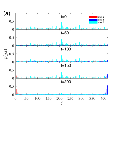
Figure 5: (a) The profiles of $p\left(j,t\right)$ at several typical instants, which is defined in Eq. (62), showing the formation of the edge state. (b) Corresponding fidelity defined in Eq. (65). The parameters are $N=140,V=0,v=5,w=3,\mu_{0}=0,W=2,\gamma=0.5,\omega=0.001.$

We define the time-dependent distribution of particle probability $p\left(j,t\right)$ in central system as

$$p\left(3l-2,t\right) = \left|\left\langle 0\right|a_{l}\left|\psi\left(t\right)\right\rangle\right|,$$

$$p\left(3l-1,t\right) = \left|\left\langle 0\right|b_{l}\left|\psi\left(t\right)\right\rangle\right|,$$

$$p\left(3l,t\right) = \left|\left\langle 0\right|d_{l}\left|\psi\left(t\right)\right\rangle\right|,$$ (62)

for the evolved state to measure the efficiency of the scheme. Ideally, the target state with perfect edge state has the distribution $p_{\mathrm{E}}\left(j\right)$

$$p_{\mathrm{E}}\left(3l-2\right) = \Omega^{2}\left(\frac{w}{v}\right)^{4l-2},$$

$$p_{\mathrm{E}}\left(3l-1\right) = \Omega^{2}\left(\frac{w}{v}\right)^{2N-2l},$$

$$p_{\mathrm{E}}\left(3l\right) = 0.$$ (63)

In the case with non-uniform distributions $\left\{w_{j}\right\}$ and $\left\{v_{j}\right\}$, the corresponding $p_{\mathrm{E}}$ can be obtained numerically from exactly diagonalization of the Hamiltonian. Numerical simulations for the formation processes of the single-particle edge state in the absence and presence of random perturbations with different random strengths. The computation is performed by taking two sets of random numbers $\left\{w_{j}\right\}$ and $\left\{v_{j}\right\}$ around $w$ and $v$, i.e.,

$$w_{j}=w+\mathrm{ran}(-R,R),v_{j}=v+\mathrm{ran}(-R,R),$$ (64)

where $\mathrm{ran}(-R,R)$ denotes a uniform random number within $(-R,R)$. We employ the fidelity

$$f(t)=\left|\langle\psi_{\text{T}}\left|\psi\left(t\right)\right\rangle\right|$$ (65)

to characterize the efficiency of the scheme, where the target state $\left|\psi_{\text{T}}\right\rangle$ is the midgap state. The profiles of $p\left(j,t\right)$ for several representative situations with fixed $w$ and $v$ are presented in Fig. 5 and with different random strengths $\left\{w_{j}\right\}$ and $\left\{v_{j}\right\}$ are presented in Fig. 6. We can see that the evolved state with fixed $w$ and $v$ very closes to the perfect edge state. In presence of random perturbations, although the probability distribution seems irregular, it is evidently edge state. These results accord with our predictions. This scheme can be extended to the cases with $2$D and $3$D central systems for preparing edge and surface states. Unlike the bulk states, these states are responsible for the topological features.

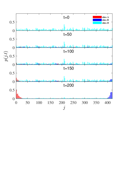
Figure 6: The profiles of $p\left(j,t\right)$ at several typical instants in the presence of random perturbations with different random strengths $w_{j}$ and $v_{j}$ defined in Eq. (64). The parameters are $N=140,V=0,v=5,w=3,\mu_{0}=0,W=2,\gamma=0.5,\omega=0.001,R=1.2.$

V Summary

In summary, we present a scheme to realize the quantum mold casting, i.e., engineering a target quantum state on demand by the time evolution of a trivial initial state. The underlying mechanism is EP dynamics. We have proposed a quantum mold model for dynamically casting a stable topological insulating states and edge states. We introduce the periodic driving chemical potential which causes EPs to exist in different subspaces, and allows fermions be transferred from the full-filled trivial source system to the corresponding subspaces of the topological central system. As examples, we consider the central system as the QWZ model and generalized RM model to dynamic casting topological insulating states and edge states, respectively. Numerical simulations show that the scheme is efficient. The advantage of the scheme is that the robust topological edge and surface states can be engineered without filling the whole valence band.

References

- (1) T. Oka and H. Aoki, Photovoltaic Hall effect in graphene, Phys. Rev. B 79, 081406(R) (2009).
- (2) T. Kitagawa, T. Oka, A. Brataas, L. Fu, and E. Demler, Transport properties of nonequilibrium systems under the application of light: Photoinduced quantum Hall insulators without Landau levels, Phys. Rev. B 84, 235108 (2011).
- (3) M. S. Rudner, N. H. Lindner, E. Berg, and M. Levin, Anomalous edge states and the bulk-edge correspondence for periodically driven two-dimensional systems, Phys. Rev. X 3, 031005 (2013).
- (4) L. E. F. Foa Torres, P. M. Perez-Piskunow, C. A. Balseiro, and G. Usaj, Multiterminal conductance of a Floquet topological insulator, Phys. Rev. Lett. 113, 266801 (2014).
- (5) H. Dehghani, T. Oka, and A. Mitra, Out-of-equilibrium electrons and the Hall conductance of a Floquet topological insulator, Phys. Rev. B 91, 155422 (2015).
- (6) J. H. Wilson, J. C.W. Song, and G. Refael, Remnant geometric Hall response in a quantum quench, Phys. Rev. Lett. 117, 235302 (2016).
- (7) N. H. Lindner, G. Refael, and V. Galitski, Floquet topological insulator in semiconductor quantum wells, Nat. Phys. 7, 490 (2011).
- (8) J. Cayssol, B. Dora, F. Simon, and R. Moessner, Floquet topological insulators, Phys. Status Solidi R 7, 101 (2013).
- (9) M. Thakurathi, A. A. Patel, D. Sen, and A. Dutta, Floquet generation of Majorana end modes and topological invariants, Phys. Rev. B 88, 155133 (2013).
- (10) A. Kundu and B. Seradjeh, Transport signatures of Floquet Majorana fermions in driven topological superconductors, Phys. Rev. Lett. 111, 136402 (2013).
- (11) C. M. Bender and S. Boettcher, Real spectra in non-Hermitian Hamiltonians having PT symmetry, Phys. Rev. Lett. 80, 5243 (1998).
- (12) C. M. Bender, D. C. Brody, and H. F. Jones, Complex extension of quantum mechanics, Phys. Rev. Lett. 89, 270401 (2002).
- (13) A. Mostafazadeh, Pseudo-Hermiticity versus PT-symmetry: The necessary condition for the reality of the spectrum of a non-Hermitian Hamiltonian, J. Math. Phys. 43, 205 (2002); Pseudo-Hermiticity versus PT symmetry: The necessary condition for the reality of the spectrum of a non-Hermitian Hamiltonian, J. Math. Phys. 43, 2814; Pseudo-Hermiticity versus PT-symmetry. II. A complete characterization of non-Hermitian Hamiltonians with a real spectrum, J. Math. Phys. 43, 3944 (2002); Pseudo-supersymmetric quantum mechanics and isospectral pseudo-Hermitian Hamiltonians, Nucl. Phys. B 640, 419 (2002); Pseudo-Hermiticity and generalized PT- and CPT-symmetries, J. Math. Phys. 44, 974 (2003).
- (14) W. D. Heiss, The physics of exceptional points, J. Phys. A: Math. Theor. 45, 444016 (2012).
- (15) I. Rotter, A non-Hermitian Hamilton operator and the physics of open quantum systems, J. Phys. A: Math. Theor. 42, 153001 (2009); I. Rotter and A. F. Sadreev, Avoided level crossings, diabolic points, and branch points in the complex plane in an open double quantum dot, Phys. Rev. E 71, 036227 (2005).
- (16) H. Xu, D. Mason, L. Jiang and J. G. E. Harris, Topological energy transfer in an optomechanical system with exceptional points, Nature 537, 80 (2016).
- (17) B. F. Samsonov, Spectral singularities of non-Hermitian Hamiltonians and SUSY transformations, J. Phys. A: Math. Gen. 38, 571 (2005).
- (18) A. A. Andrianov, F. Cannata, and A. V. Sokolov. Spectral singularities for non-Hermitian one-dimensional Hamiltonians: puzzles with resolution of identity, J. Math. Phys. 51, 052104 (2010).
- (19) A. Mostafazadeh, Spectral singularities of complex scattering potentials and infinite reflection and transmission coefficients at real energies, Phys. Rev. Lett. 102, 220402 (2009); Optical spectral singularities as threshold resonances, Phys. Rev. A 83, 045801 (2011).
- (20) S. Longhi, Spectral singularities in a non-Hermitian Friedrichs-Fano-Anderson model, Phys. Rev. B 80, 165125 (2009); Spectral singularities and Bragg scattering in complex crystals, Phys. Rev. A 81, 022102 (2010).
- (21) X. Z. Zhang, L. Jin, and Z. Song, Perfect state transfer in PT-symmetric non-Hermitian networks, Phys. Rev. A 85, 012106 (2012).
- (22) X. Z. Zhang, L. Jin, and Z. Song, Dynamic magnetization in non-Hermitian quantum spin systems, Phys. Rev. B 101, 224301 (2020).
- (23) X. Z. Zhang and Z. Song, Dynamical preparation of a steady ODLRO state in the Hubbard model with local non-Hermitian impurity, arXiv:2009.06167.
- (24) X. M. Yang and Z. Song, Resonant generation of a p-wave Cooper pair in a non-Hermitian Kitaev chain at the exceptional point, Phys. Rev. A 102, 022219 (2020).
- (25) X.-L. Qi, Y.-S. Wu, and S.-C. Zhang, Topological quantization of the spin hall effect in two-dimensional paramagnetic semiconductors, Phys. Rev. B 74, 085308 (2006).
- (26) S. Lin and Z. Song, Wide-range-tunable Dirac-cone band structure in a chiral-time-symmetric non-Hermitian system, Phys. Rev. A 96, 052121 (2017).
- (27) S. Ryu and Y. Hatsugai, Topological Origin of Zero-Energy Edge States in Particle-Hole Symmetric Systems, Phys. Rev. Lett. 89, 077002 (2002).
- (28) X.-G. Wen, Symmetry-protected topological phases in noninteracting fermion systems, Phys. Rev. B 85, 085103 (2012).
- (29) D. Xiao, M. C. Chang, and Q. Niu, Berry phase effects on electronic properties, Rev. Mod. Phys. 82, 1959 (2010).
- (30) M. Z. Hasan and C. L. Kane, Colloquium: Topological insulators, Rev. Mod. Phys. 82, 3045 (2010); X.-L. Qi and S.-C. Zhang, Topological insulators and superconductors, Rev. Mod. Phys. 83, 1057 (2011).
- (31) P. Delplace, D. Ullmo, and G. Montambaux, Zak phase and the existence of edge states in graphene, Phys. Rev. B 84, 195452 (2011).
- (32) L. Li, Z. Xu, and S. Chen, Topological phases of generalized Su-Schrieffer-Heeger models, Phys. Rev. B 89, 085111 (2014).
- (33) L. Li and S. Chen, Characterization of topological phase transitions via topological properties of transition points, Phys. Rev. B 92, 085118 (2015).
- (34) S. Lin, X. Z. Zhang, C. Li, and Z. Song, Long-range entangled zero-mode state in a non-Hermitian lattice, Phys. Rev. A 94, 042133 (2016).
- (35) R. Wang and Z. Song, Dynamical topological invariant for the non-Hermitian Rice-Mele model, Phys. Rev. A 98, 042120 (2018).
- (36) R. Wang and Z. Song, Robustness of the pumping charge to dynamic disorder, Phys. Rev. B 100, 184304 (2019).