3D Simulations of Oxygen Shell Burning with and without Magnetic Fields

Abstract

We present a first 3D magnetohydrodynamic (MHD) simulation of convective oxygen and neon shell burning in a non-rotating $18\,M_{\odot}$ star shortly before core collapse to study the generation of magnetic fields in supernova progenitors. We also run a purely hydrodynamic control simulation to gauge the impact of the magnetic fields on the convective flow and on convective boundary mixing. After about 17 convective turnover times, the magnetic field is approaching saturation levels in the oxygen shell with an average field strength of $\mathord{\sim}10^{10}\,\mathrm{G}$, and does not reach kinetic equipartition. The field remains dominated by small to medium scales, and the dipole field strength at the base of the oxygen shell is only $10^{9}\,\mathrm{G}$. The angle-averaged diagonal components of the Maxwell stress tensor mirror those of the Reynolds stress tensor, but are about one order of magnitude smaller. The shear flow at the oxygen-neon shell interface creates relatively strong fields parallel to the convective boundary, which noticeably inhibit the turbulent entrainment of neon into the oxygen shell. The reduced ingestion of neon lowers the nuclear energy generation rate in the oxygen shell and thereby slightly slows down the convective flow. Aside from this indirect effect, we find that magnetic fields do not appreciably alter the flow inside the oxygen shell. We discuss the implications of our results for the subsequent core-collapse supernova and stress the need for longer simulations, resolution studies, and an investigation of non-ideal effects for a better understanding of magnetic fields in supernova progenitors.

1 Introduction

Rigorous three-dimensional (3D) simulations of neutrino-driven core-collapse supernovae have become highly successful in recent years (e.g., Melson et al., 2015; Lentz et al., 2015; Takiwaki et al., 2014; Burrows et al., 2019), and have made clear headway in explaining the properties of supernova explosions and the compact objects born in these events (Müller et al., 2017; Müller et al., 2019; Burrows et al., 2020; Powell & Müller, 2020; Bollig et al., 2020; Müller, 2020). The latest 3D models are able to reproduce a range of explosion energies up to $10^{51}\mathrm{erg}$ (Bollig et al., 2020), and yield neutron star birth masses, kicks, and spins largely compatible with the population of observed young pulsars (Müller et al., 2019; Burrows et al., 2020).

A number of ingredients have contributed, or have the potential to contribute, to make modern neutrino-driven explosion models more robust. Various microphysical effects such as reduced neutrino scattering opacities due to nucleon strangeness (Melson et al., 2015) and nucleon correlations at high densities (Horowitz et al., 2017; Bollig et al., 2017; Burrows et al., 2018), muonisation (Bollig et al., 2017), and large effective nucleon masses (Yasin et al., 2020) can be conducive to neutrino-driven shock revival.

In addition, a particularly important turning point has been the advent of 3D progenitor models and the recognition that asphericities seeded prior to collapse can precipitate “perturbation-aided” neutrino-driven explosions (Couch & Ott, 2013; Couch et al., 2015; Müller & Janka, 2015; Müller, 2016; Müller et al., 2017; Müller, 2020; Bollig et al., 2020). In perturbation-aided explosions, the moderately subsonic solenoidal velocity perturbation in active convective shells at the pre-collapse stage with Mach numbers of order $\mathord{\sim}0.1$ (Collins et al., 2018) are transformed into strong density and pressure perturbations at the shock (Müller & Janka, 2015; Takahashi & Yamada, 2014; Takahashi et al., 2016; Abdikamalov & Foglizzo, 2020), and effectively strengthen the violent non-radial flow behind the shock that develops due to convective instability (Herant et al., 1994; Burrows et al., 1995; Janka & Müller, 1995, 1996) and the standing accretion shock instability (Blondin et al., 2003; Foglizzo et al., 2007), thereby supporting neutrino-driven shock revival.

The discovery of perturbation-aided explosions has greatly enhanced interest in multi-dimensional models of late convective burning stages in massive stars. Several studies have by now followed the immediate pre-collapse phase of silicon and/or oxygen shell burning to collapse in 3D (Couch et al., 2015; Müller, 2016; Müller et al., 2016; Müller et al., 2019; Yoshida et al., 2019; Yadav et al., 2020; McNeill & Müller, 2020; Yoshida et al., 2020). In addition, there has been a long-standing strand of research since the 1990s (e.g., Bazan & Arnett, 1994; Bazán & Arnett, 1997; Meakin & Arnett, 2006, 2007b, 2007a; Müller et al., 2016; Jones et al., 2017; Cristini et al., 2017, 2019) into the detailed behaviour of stellar convection during advanced burning stages with a view to the secular impact of 3D effects not captured by spherically symmetric stellar evolution models based on mixing-length theory (Biermann, 1932; Böhm-Vitense, 1958). The details of convective boundary mixing by processes such as quasi-steady turbulent entrainment (Fernando, 1991; Strang & Fernando, 2001; Meakin & Arnett, 2007b) or violent shell mergers (Mocák et al., 2018; Yadav et al., 2020) have received particular attention for their potential to alter the core structure of massive stars and hence affect the dynamics and final nucleosynthesis yields of the subsequent supernova explosion.

Three-dimensional simulations of convection during advanced burning stages have so far largely disregarded two important aspects of real stars – rotation and magnetic fields. The effects of rotation have been touched upon by the seminal work of Kuhlen et al. (2003), but more recent studies (Arnett & Meakin, 2010; Chatzopoulos et al., 2016) have been limited to axisymmetry (2D). Magnetohydrodynamic (MHD) simulations of convection, while common and mature in the context of the Sun (for a review see, e.g., Charbonneau, 2014) have yet to be performed for advanced burning stages of massive stars.

Simulations of magnetoconvection during the late burning stages, both in rotating and non-rotating stars, are a big desideratum for several reasons. Even in slowly rotating massive stars, magnetic fields may have a non-negligible impact on the dynamics of neutrino-driven explosions (Obergaulinger et al., 2014; Müller & Varma, 2020), and although efficient field amplification processes operate in the supernova core (Endeve et al., 2012; Müller & Varma, 2020), it stands to reason that memory of the initial fields may not be lost entirely, especially for strong fields in the progenitor and early explosions. A better understanding of the interplay between convection, rotation, and magnetic fields in supernova progenitors is even more critical for the magnetorotational explosion scenario (e.g., Burrows et al., 2007; Winteler et al., 2012; Mösta et al., 2014; Mösta et al., 2018; Obergaulinger & Aloy, 2020a, b; Kuroda et al., 2020; Aloy & Obergaulinger, 2020), which probably explains rare, unusually energetic “hypernovae” with energies of up to $\mathord{\sim}10^{52}\,\mathrm{erg}$. Again, even though the requisite strong magnetic fields may be generated after collapse by amplification processes like the magnetorotational insstability (Balbus & Hawley, 1991; Akiyama et al., 2003) or an $\alpha$-$\Omega$ dynamo in the proto-neutron star (Duncan & Thompson, 1992; Thompson & Duncan, 1993; Raynaud et al., 2020), a robust understanding of magnetic fields during late burning is indispensable for reliable hypernova models on several heads. For sufficiently strong seed fields in the progenitor, the initial field strengths and geometry could have a significant impact on the development of magnetorotational explosions after collapse (Bugli et al., 2020; Aloy & Obergaulinger, 2020). Furthermore, our understanding of evolutionary pathways towards hypernova explosions (Woosley & Heger, 2006; Yoon & Langer, 2005; Yoon et al., 2010; Cantiello et al., 2007; Aguilera-Dena et al., 2018, 2020) is intimately connected with the effects of magnetic fields on angular momentum transport in stellar interiors (Spruit, 2002; Heger et al., 2005; Fuller et al., 2019; Takahashi & Langer, 2020).

Beyond the impact of magnetic fields on the pre-supernova evolution and the supernova itself, the interplay of convection, rotation, and magnetic fields is obviously relevant to the origin of neutron star magnetic fields as well. It still remains to be explained what shapes the distribution of magnetic fields among young pulsars, and why some neutron stars are born as magnetars with extraordinarily strong dipole fields of up to $10^{15}\,\mathrm{G}$ (Olausen & Kaspi, 2014; Tauris et al., 2015; Kaspi & Beloborodov, 2017; Enoto et al., 2019). Are these strong fields of fossil origin (Ferrario & Wickramasinghe, 2005; Ferrario et al., 2009; Schneider et al., 2020) or generated by dynamo action during or after the supernova (Duncan & Thompson, 1992; Thompson & Duncan, 1993)? Naturally, 3D MHD simulations of the late burning stages cannot comprehensively answer all of these questions. In order to connect to observable magnetic fields of neutron stars, an integrated approach is required that combines stellar evolution over secular time scales, 3D stellar hydrodynamics, supernova modelling, and local simulations, and also addresses aspects like field burial (Viganò et al., 2013; Torres-Forné et al., 2016) and the long-time evolution of magnetic fields (Aguilera et al., 2008; De Grandis et al., 2020). Significant obstacles need to be overcome until one can construct a pipeline from 3D progenitor models to 3D supernova simulations and beyond. However, 3D MHD simulations of convective burning can already address meaningful questions despite the complexity of the overall problem. As in the purely hydrodynamic case, the first step must be to understand the principles governing magnetohydrodynamic convection during the late burning stages based on somewhat idealised simulations that are broadly representative of the conditions in convective cores and shells of massive stars.

In this study, we present a first simulation of magnetoconvection during the final phase of oxygen shell burning using the ideal MHD approximation. In the tradition of semi-idealised models of late-stage convection, we use a setup that falls within the typical range of conditions in the interiors of massive stars in terms of convective Mach number and shell geometry (for an overview see Collins et al., 2018) and is not designed as a fully self-consistent model of any one particular star. This simulation constitutes a first step beyond effective 1D prescriptions in stellar evolution models to predict the magnetic field strength and geometry encountered in the inner shells of massive stars at the pre-supernova stage. We also compare to a corresponding non-magnetic model of oxygen shell convection to gauge the feedback of magnetic fields on the convective flow with a particular view to two important issues. First, the efficiency of the “perturbation-aided” neutrino-driven mechanism depends critically on the magnitude of the convective velocities during shell burning, and it is important to determine whether magnetic fields can significantly slow down convective motions as suggested by some recent simulations of solar convection (Hotta et al., 2015). Second, magnetic fields could quantitatively or qualitatively affect shell growth by turbulent entrainment, which has been consistently seen in all recent 3D hydrodynamics simulations of late-stage convection in massive stars.

Our paper is structured as follows. In Section 2, we describe the numerical methods, progenitor model, and initial conditions used in our study and discuss the potential role of non-ideal effects . The results of the simulations are presented in Section 3. We first focus on the strength and geometry of the emerging magnetic field and then analyse the impact of magnetic fields on the flow, and in particular on entrainment at shell boundaries. We summarize our results and discuss their implications in Section 4.

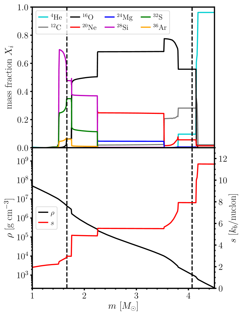
Figure 1: Profiles of selected mass fractions $X_{i}$ (top), density $\rho$, and specific entropy $s$ in the $18\,M_{\odot}$ Kepler stellar evolution model at the time of mapping to CoCoNuT. The boundaries of the simulated domain are indicated by dashed vertical lines. Note subtle differences to Figure 1 in Müller et al. (2016), which shows the same stellar evolution model at the onset of collapse.

2 Numerical Methods and Simulation Setup

We simulate oxygen and neon shell burning with and without magnetic fields in a non-rotating $18\,M_{\odot}$ solar-metallicity star calculated using the stellar evolution code Kepler (Weaver et al., 1978; Woosley et al., 2002; Heger & Woosley, 2010). The same progenitor model has previously been used in the shell convection simulation of Müller et al. (2016). The structure of the stellar evolution model at the time of mapping to 3D is illustrated in Figure 1. The model contains two active convective shells with sufficiently short turnover times to make time-explicit simulations feasible. The oxygen shell extends from $1.75\,M_{\odot}$ to $2.25\,M_{\odot}$ in enclosed mass and from $3,400\,\mathrm{km}$ to $7,900\,\mathrm{km}$ in radius, immediately followed further out by the neon shell out to $3.53\,M_{\odot}$ in mass and $27,000\,\mathrm{km}$ in radius.

For our 3D simulations we employ the Newtonian magnetohydrodynamic (MHD) version of the CoCoNuT code as described in Müller & Varma (2020). The MHD equations are solved in spherical polar coordinates using the HLLC (Harten-Lax-van Leer-Contact) Riemann solver (Gurski, 2004; Miyoshi & Kusano, 2005). The divergence-free condition $\nabla\cdot\mathbf{B}=0$ is maintained using a modification of the original hyperbolic divergence cleaning scheme of Dedner et al. (2002) that allows for a variable cleaning speed while still maintaining total energy conservation using an idea similar to Tricco et al. (2016). Compared to the original cleaning method, we rescale the Lagrange multiplier $\psi$ to $\hat{\psi}=\psi/c_{\mathrm{h}}$, where the cleaning speed $c_{\mathrm{h}}$ is chosen to be the fast magnetosonic speed. Details of this approach and differences to Tricco et al. (2016) are discussed in Appendix A. The extended system of MHD equations for the density $\rho$, velocity $\mathbf{v}$, magnetic field $\mathbf{B}$, the total energy density $\hat{e}$, mass fractions $X_{i}$, and the rescaled Lagrange multiplier $\hat{\psi}$ reads,

$$\partial_{t}\rho+\nabla\cdot\rho\mathbf{v} = 0,$$ (1)

$$\partial_{t}(\rho\mathbf{v})+\nabla\cdot\left(\rho\mathbf{v}\mathbf{v}-\frac{\mathbf{B}\mathbf{B}}{4\pi}+P_{\mathrm{t}}\mathcal{I}\right) = \rho\mathbf{g}-\frac{(\nabla\cdot\mathbf{B})\mathbf{B}}{4\pi},$$ (2)

$$\partial_{t}{\hat{e}}+\nabla\cdot\left[(e+P_{\mathrm{t}})\mathbf{u}-\frac{\mathbf{B}(\mathbf{v}\cdot\mathbf{B}){-c_{\mathrm{h}}\hat{\psi}\mathbf{B}}}{4\pi}\right] = \rho\mathbf{g}\cdot\mathbf{v}+\rho\dot{\epsilon}_{\mathrm{nuc}},$$ (3)

$$\partial_{t}\mathbf{B}+\nabla\cdot(\mathbf{v}\mathbf{B}-\mathbf{B}\mathbf{v})+\nabla(c_{\mathrm{h}}\hat{\psi}) = 0,$$ (4)

$$\partial_{t}\hat{\psi}+c_{\mathrm{h}}\nabla\cdot\mathbf{B} = -\hat{\psi}/\tau,$$ (5)

$$\partial_{t}(\rho X_{i})+\nabla\cdot(\rho X_{i}\mathbf{v}) = \rho\dot{X}_{i},$$ (6)

where $\mathbf{g}$ is the gravitational acceleration, $P_{\mathrm{t}}$ is the total pressure, $\mathcal{I}$ is the Kronecker tensor, $c_{\mathrm{h}}$ is the hyperbolic cleaning speed, $\tau$ is the damping time scale for divergence cleaning, and $\dot{\epsilon}_{\mathrm{nuc}}$ and $\dot{X}_{i}$ are energy and mass fraction source terms from nuclear reactions. This system conserves the volume integral of a modified total energy density $\hat{e}$, which also contains the cleaning field $\hat{\psi}$,

$${\hat{e}}=\rho\left(\epsilon+\frac{v^{2}}{2}\right)+\frac{B^{2}+\hat{\psi}^{2}}{8\pi},$$ (7)

where $\epsilon$ is the mass-specific internal energy. Note that the energy equation differs from that in Tricco et al. (2016) because we implement divergence cleaninng on a Eulerian grid and do not advect $\psi$ with the flow unlike in their smoothed particle hydrodynamics approach. If translated to the Eulerian form of the MHD equations, the approach of Tricco et al. (2016) would give rise to an extra advection term in the evolution equation for $\psi$, which then requires an additional term in the energy equation to ensure energy conservation. In our Eulerian approach, these extra terms are not needed.

Viscosity and resistivity are not included explicitly in the ideal MHD approximation, and only enter through the discretisation of the MHD equations, specifically the spatial reconstruction, the computation of the Riemann fluxes, and the update of the conserved quantities in the case of reconstruct-solve-average schemes. While this “implicit large-eddy simulation” (ILES) approach is well-established for hydrodynamic turbulence (Grinstein et al., 2007), the magnetohydrodynamic case is more complicated because the behaviour in the relevant astrophysical regime of low (kinematic) viscosity $\nu$ and resistivity $\eta$ may still depend on the magnetic Prandtl number $\mathrm{Pm}=\nu/\eta$. Different from the regime later encountered in the supernova core where $\mathrm{Pm}\gg 1$, oxygen shell burning is characterised by magnetic Prandtl numbers slightly below unity ($\mathrm{Pm}\sim 0.2$). With an effective Prandtl number of $\mathrm{Pm}\sim 1$ in the ILES approach (Federrath et al., 2011), there is a potential concern that spurious small-scale dynamo amplification might arise due to the overestimation of the magnetic Prandtl number, or that saturation field strengths might be too high. The debate about the magnetic Prandtl number dependence in MHD turbulence is ongoing with insights from theory and simulations (e.g., Schekochihin et al., 2004; Schekochihin et al., 2007; Iskakov et al., 2007; Brandenburg, 2011; Pietarila Graham et al., 2010; Sahoo et al., 2011; Thaler & Spruit, 2015; Seshasayanan et al., 2017), astrophysical observations (e.g., Christensen et al., 2009), and laboratory experiments (Pétrélis et al., 2007; Monchaux et al., 2007). There is, at the very least, the possibility of robust small-scale dynamo action and saturation governed by balance between the inertial terms and Lorentz force terms down to the low values of $\mathrm{Pm}\sim 5\times 10^{-6}$ in liquid sodium experiments (Pétrélis et al., 2007; Monchaux et al., 2007), provided that both the hydrodynamic and magnetic Reynolds number are sufficiently high. An ILES approach that places the simulation into a “universal”, strongly magnetised regime (Beresnyak, 2019) thus appears plausible. Moreover, even if the ILES approach were only to provide upper limits for magnetic fields and their effects on the flow, meaningful conclusions can still be drawn in the context of shell convection simulations.

The nuclear source terms are calculated with the 19-species nuclear reaction network of Weaver et al. (1978). Neutrino cooling is ignored, since it becomes subdominant in the late pre-collapse phase as the contraction of the shells speeds up nuclear burning.

The simulations are conducted on a grid with $400\times 128\times 256$ zones in radius $r$, colatitude $\theta$, and longitude $\varphi$ with an exponential grid in $r$ and uniform spacing in $\theta$ and $\varphi$. To reduce computational costs, we excise the non-convective inner core up to $3000\,\mathrm{km}$ and replace the excised core with a point mass. The grid extends to a radius of $50,000\,\mathrm{km}$ and includes a small part of the silicon shell, the entire convective oxygen and neon shells, the non-convective carbon shell, and parts of the helium shell. Simulations that include the entire iron core and silicon shell are of course desirable in future, but the treatment of nuclear quasi-equilibrium in these regions is delicate and motivates simulations in a shellular domain instead, with a sufficient “buffer” region between the convectively active shells and the inner boundary of the grid. Due to the significant buoyancy jump between the silicon shell and the oxygen shell, the flow in the convective shell is largely decoupled from that in the non-convective buffer region. Hydrodynamic waves excited at the convective boundary and Alfvén waves along field lines threading both regions can introduce some coupling, but these are excited by the active convective shell and not in the convectively quiet buffer region. No physical flux of waves into the oxygen region from below is expected. Moreover, there is no strong excitation of waves at the convective boundary in the first place because of the low convective Mach number of the flow. It turns out that coupling by Alfvén waves can be neglected even more safely than coupling by internal gravity waves because of the Alfvén number of the flow; as we shall see the Alfvén number always stays well below unity.

In order to investigate the impact of magnetic fields on late-stage oxygen shell convection, we run a purely hydrodynamic, non-magnetic simulation and an MHD simulation. In the MHD simulation, we impose a homogeneous magnetic field with $B_{z}=10^{8}\,\mathrm{G}$ parallel to the grid axis as initial conditions. We implement reflecting and periodic boundary conditions in $\theta$ and $\varphi$, respectively. For the hydrodynamic variables we use hydrostatic extrapolation (Müller, 2020) at the inner and outer boundary, and impose strictly vanishing advective fluxes at the inner boundary. Different from Müller et al. (2016), we do not contract the inner boundary to follow the contraction and collapse of the core. This means that our models will not (and are not intended to) provide an accurate representation of the pre-collapse state of the particular $18M_{\odot}$ star that we are simulating. We would expect, e.g., that for the particular $18M_{\odot}$ model, the burning rate and hence the convective velocities would increase until the onset of collapse (Müller et al., 2016) due to the contraction of the convective oxygen shell. As a consequence of accelerating convection and flux compression, the magnetic fields will likely also be somewhat higher at the onset of collapse. The model is rather meant to reveal the physical principles governing late-stage magnetoconvection in massive stars, and to be representative of the typical conditions in oxygen burning shells with the understanding that there are significant variations in convective Mach number and shell geometry at the onset of collapse (Collins et al., 2018), which will also be reflected in the magnetic field strengths in the interiors of supernova progenitors.

The inner and outer boundary conditions for the magnetic fields are less trivial. In simulations of magnetoconvection in the Sun, various choices such as vertical boundary conditions ($B_{x}=B_{y}=0$), radial boundary conditions ($B_{\theta}=B_{\varphi}=0$), vanishing tangential electric fields or currents, perfect-conductor boundary conditions, or extrapolation to a potential solution have been employed (e.g., Thelen & Cattaneo, 2000; Rempel, 2014; Käpylä et al., 2020). Since our domain boundaries are separated from the convective regions by shell interfaces with significant buoyancy jumps, we opt for the simplest choice of boundary conditions and merely fix the magnetic fields in the ghost zones to their initial values for a homogeneous vertical magnetic field. We argue that due to the buffer regions at our radial boundaries, and the lack of rotational shear, our choice of magnetic boundary conditions should not have a significant impact on the dynamically relevant regions of the star.

3 Results

3.1 Evolution of the Magnetic Field

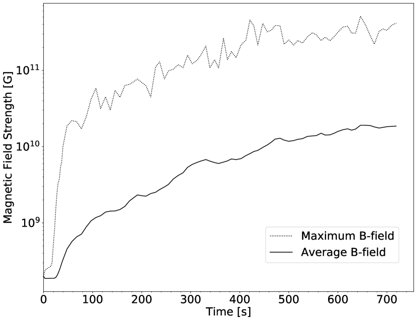
Figure 2: Evolution of the volume-averaged (solid) and maximum (dashed) magnetic field strength within the oxygen shell.

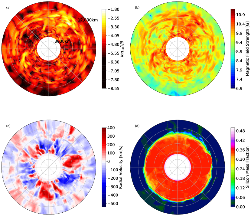
Figure 3: Snapshots of the equatorial plane in the MHD simulation at a time of $500\,\mathrm{s}$, showing the inner part of the domain from the inner boundary at a radius of $3000\,\mathrm{km}$ out to $12,000\,\mathrm{km}$. The plotted part of the domain corresponds to the range $\mathrm{1.67\,M_{\odot}-2.54\,M_{\odot}}$ in mass coordinate.

The panels display a) the ratio of magnetic to thermal pressure (i.e., inverse plasma-$\beta$), b) the magnitude of the magnetic field strength, c) the radial velocity and d) the silicon mass fraction.

Both the magnetised and non-magnetised model were run for over 12 minutes of physical time, which corresponds to about 17 convective turnover times. Very soon after convection develops in the oxygen shell, the turbulent convective flow starts to rapidly amplify the magnetic fields in this region. To illustrate the growth of the magnetic field we show the root-mean-square (RMS) average and maximum value of the magnetic field in the oxygen shell in Figure 2.The magnetic field, which we initialised at $10^{8}\,\mathrm{G}$, is amplified by over two orders of magnitude to over $10^{10}\,\mathrm{G}$ on average within the shell due to convective and turbulent motions. The average magnetic field strength in the shell is still increasing at the end of the simulation, but the growth rate has slowed down, likely indicating that the model is approaching some level of magnetic field saturation. While we cannot with certainty extrapolate the growth dynamics without simulating longer, it appears likely that RMS saturation field strength will settle somewhere around $\mathord{\approx}2\times 10^{10}\,\mathrm{G}$.

A closer look reveals that the magnetic field is not amplified homogeneously throughout the convective region. The convective eddies push the magnetic field lines against the convective boundaries, where the fields are then more strongly amplified by shear flows. This is visualised in Figures 3a and 3b, where both magnetic pressure and magnetic field strengths appear concentrated at the convective boundary. The maximum magnetic field strength shown in Figure 2 (dashed line) therefore essentially mirrors the field at the inner boundary of the oxygen shell (not to be confused with the inner grid boundary). We observe a very quick rise in magnetic field strength at the boundary at the beginning of the simulation between $20\texttt{-}50\,\mathrm{s}$ once the convective flow is fully developed. The rate of growth of the maximum magnetic field strength after this increases at approximately the same rate as the average magnetic field strength.

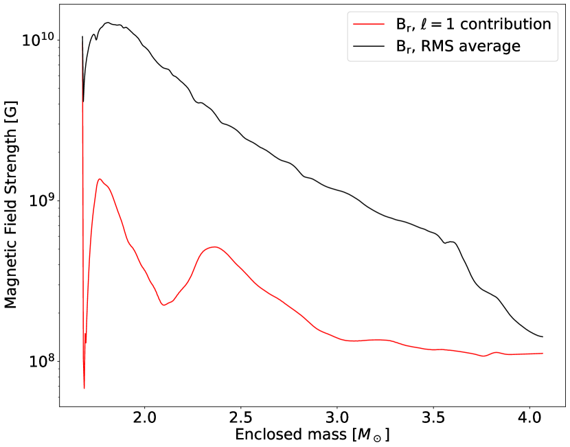
Figure 4: The angle-averaged root-mean-square (RMS) value (black) and the dipole component (red) of the radial magnetic field component $B_{r}$ as a function of mass coordinate at a time of $725\,\mathrm{s}$. Note that the magnetic field strength drops dramatically inside the thin, convectively stable buffer region below the oxygen shell, but exhibits a peak in the first radial zone, which is merely a numerical artefact due to imperfect boundary conditions.

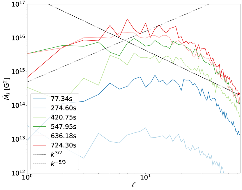
Figure 5: Power $\hat{M}_{\ell}^{2}$ in different multipoles $\ell$ of the radial field component of the magnetic field in the oxygen shell at different times. Dotted lines show the slopes of Kolmogorov ($k^{-5/3}$) and Kazantsev ($k^{3/2}$) spectra. The low-wavenumber part of the spectrum is always distinctly flatter than a Kazantsev spectrum; at intermediate $\ell$, we see a Kolmogorov-like spectrum with a break around $\ell=30$ to a steeper slope in the dissipation range.

To characterise the geometric structure of the magnetic field, we show a radial profile of the dipole of the radial magnetic field component $B_{r}$ at the end of the simulation at $\approx 725\,\mathrm{s}$ (Figure 4). The dipole magnetic field in the convective regions is approximately an order of magnitude smaller than the RMS average radial magnetic field, aside from the first radial zone of our grid, where the dipole component is comparable to the total radial magnetic field. This behaviour at the grid boundary is likely an artefact of our choice of homogeneous magnetic fields at the inner boundary. In general, however, the magnetic fields in the convective zones appear dominated by higher-order multipoles. Disregarding the dipole fields at the inner boundary, the dipole magnetic field of $\mathord{\approx}10^{9}\mathrm{G}$ or below lies in the upper range of observed dipole magnetic fields of white dwarfs (Ferrario et al., 2015), which have often been taken as best estimates for the dipole fields in the cores of massive stars.

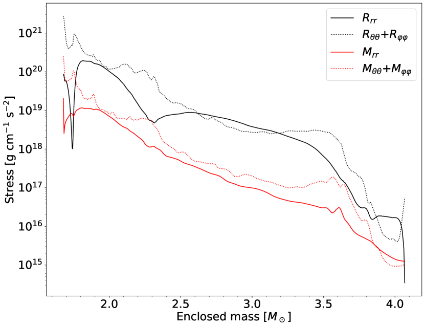
Figure 6: The radial (solid) and non-radial (dashed) diagonal components of the Reynolds stress tensor $R_{ij}$ (black) and Maxwell tensor $M_{ij}$ (red) for the MHD convection model at $725\,\mathrm{s}$ as a function of enclosed mass.

To further illustrate the small-scale nature of the magnetic field within the oxygen shell, we show angular power spectra, $\hat{M}_{\ell}$ of the radial field strength at different times as a function of the spherical harmonics degree $\ell$ inside the oxygen shell at a radius of $\mathord{\approx}5000\mathrm{km}$ (Figure 5). $\hat{M}_{\ell}$ is computed as:

$$\hat{M}_{\ell} = \frac{1}{8\pi}\sum_{m=-\ell}^{\ell}\left|\int Y_{\ell m}^{*}(\theta,\varphi)B_{r}\mathrm{d}\Omega\right|^{2}.$$ (8)

Very early in the simulation, the spectrum shows a significant $\ell=1$ dipole contribution, caused by our choice of homogeneous magnetic fields as an initial condition. It takes several convective turnovers before this contribution is no longer dominant. Throughout the evolution, the spectrum shows a broad plateau at small $\ell$ and a Kolmogorov-like slope at intermediate $\ell$, which can be more clearly distinguished at late times when the first break in the spectrum has moved towards lower $\ell$. High-resolution studies are desirable to extend the inertial range and confirm the development of a Kolmogorov spectrum at intermediate wave numbers. The break in the spectrum moves towards smaller wave numbers and the peak of the spectrum shifts to larger scales from $\ell\approx 12$ to $\ell\approx 7$. Simulations of field amplification by a small-scale dynamo in isotropic turbulence often exhibit a Kazantsev spectrum with power-law index $k^{-3/2}$ on large scales. Our spectra show a distinctly flatter slope below the spectral speak, indicating that field amplification is subtly different from the standard picture of turbulent dynamo amplification.

This is borne out by a closer look at the magnetic field distribution within the convective region. Somewhat similar to our recent simulation of field amplification by neutrino-driven convection in core-collapse supernovae (Müller & Varma, 2020), field amplification does not happen homogeneously throughout the convective region and appears to be predominantly driven by shear flows at the convective boundaries. To illustrate this, we compare the spherically-averaged diagonal components of the kinetic (Reynolds) and magnetic (Maxwell) stress tensors $R_{ij}$ and $M_{ij}$ in the MHD model at the final time-step of the simulation at $\mathord{\approx}725\,\mathrm{s}$ (Figure 6). $R_{ij}$ and $M_{ij}$ are computed as

$$R_{ij} = \langle\rho v_{i}v_{j}\rangle,$$ (9)

$$M_{ij} = \frac{1}{8\pi}\langle B_{i}B_{j}\rangle,$$ (10)

where angled brackets denote volume-weighted averages. The magnetic fields clearly remain well below equipartition with the total turbulent kinetic energy, and appear to converge to saturation levels about one order of magnitude below, although longer simulations will be required to confirm this. The non-radial diagonal components $R_{\theta\theta}+R_{\varphi\varphi}$ and $M_{\theta\theta}+M_{\varphi\varphi}$ are generally higher than the respective radial components $R_{rr}$ and $M_{rr}$. Throughout most of the domain, the Maxwell stresses are considerably smaller than the Reynolds stresses, but it is noteworthy that the profile of the non-radial components of $M_{ij}$ runs largely parallel to those of $R_{ij}$, just with a difference of slightly more than an order of magnitude. Peaks of the magnetic stresses at the shell interfaces suggest that field amplification is driven by shear flow at the convective boundaries. Convective motions then transport the magnetic field into the interior of the convective regions and also generate radial field components. The humps of $M_{rr}$ within the convection zones are less pronounced than in $R_{rr}$, which indicates that little amplification by convective updrafts and downdrafts takes place within the convection region.

At the outer boundaries of the oxygen and neon shell, we observe rough equipartition between $R_{rr}$ and $M_{\theta\theta}+M_{\varphi\varphi}$. The fact that the growth of the field slows down once the model approaches $M_{\theta\theta}+M_{\varphi\varphi}\approx R_{rr}$ suggests that this “partial equipartition” may determine the saturation field strength, but the very different behaviour at the inner boundary with $M_{\theta\theta}+M_{\varphi\varphi}\gg R_{rr}$ argues against this. It is plausible, though, that the saturation field strength is (or rather will be) determined at the boundary. Linear stability analysis of the magnetised Kelvin-Helmholtz instability (e.g. Chandrasekhar, 1961; Sen, 1963; Fejer, 1964; Miura & Pritchett, 1982; Frank et al., 1996; Keppens et al., 1999; Ryu et al., 2000; Obergaulinger, M. et al., 2010; Liu et al., 2018) shows that shear instability, which is critical for efficiently generating small-scale fields, are suppressed by magnetic fields parallel to the direction of the shear flow as long as the Alfvén number is smaller than two. With kinetic fields well below equipartition (cp. Figure 6), our models fall into the regime of low Alfvén number; hence the generation of non-radial fields at the boundaries may be self-limiting as a result of the stabilising impact of magnetic fields on the Kelvin-Helmholtz instability. A naive application of the principle of marginal stability would suggest saturation occurs once the Alfvén velocity at the boundary equals the shear velocity jump across the shell interface, which would imply $M_{\theta\theta}+M_{\varphi\varphi}\approx R_{\theta\theta}+R_{\varphi\varphi}$. Our simulation suggests that saturation probably occurs at significantly smaller values, and a more quantitative analysis of the saturation mechanism will clearly be required in future to elucidate the relation between the shear velocity (and possibly the width of the shear layer) and the saturation field strength.

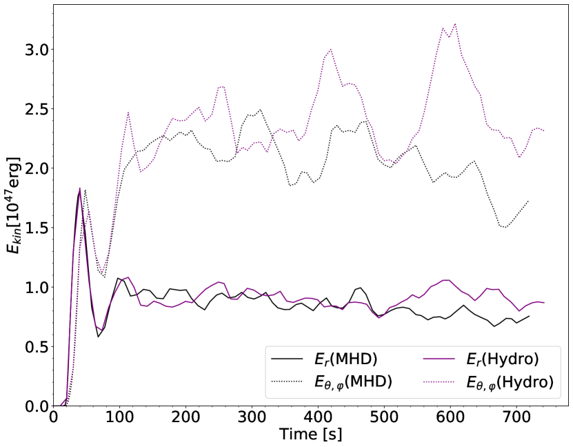
Figure 7: Evolution of the total radial (solid) and non-radial (dashed) convective kinetic energy within the oxygen shell for the purely hydrodynamic (purple) and MHD (black) model, respectively.

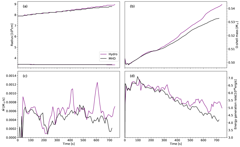
Figure 8: Effects of entrainment on the oxygen shell for both the MHD model (black) and the equivalent purely hydrodynamic model (purple). The panels show a) the inner and outer oxygen shell radii, b) the total mass within the oxygen shell, c) the entrainment rate $\dot{M}$ into the oxygen shell, and d) the volume-integrated nuclear energy generation rate throughout the shell..

3.2 Impact of Magnetic Fields on Convective Boundary Mixing

The slowing growth of the magnetic field indicates that feedback effects on the flow should become important during the later phase of the simulation. It is particularly interesting to consider the effect of the strong fields tangential to the oxygen-neon shell interface on convective boundary mixing, though we also consider potential effects on the flow in the interior of the convective regions.

To this end, we compare the MHD model to a purely hydrodynamic simulation of oxygen and neon shell convection. Figure 7 compares the total kinetic energy in convective motions in the oxygen shell between the models. The radial and non-radial components $E_{r}$ and $E_{\theta,\varphi}$ of the kinetic energy are defined as

$$E_{r} = \frac{1}{2}\int\limits_{r_{-}\leq r\leq r_{+}}\rho v_{r}^{2}\,\mathrm{d}V,$$ (11)

$$E_{\mathrm{\theta,\varphi}} = \frac{1}{2}\int\limits_{r_{-}\leq r\leq r_{+}}\rho(v_{\mathrm{\theta}}^{2}+v_{\mathrm{\varphi}}^{2})\,\mathrm{d}V,$$ (12)

where $r_{-}$ and $r_{+}$ are the inner and outer radii of the oxygen shell. We compute the inner and outer shell radii $r_{-}$ and $r_{+}$ as the midpoints of the steep, entropy slope between the oxygen shell and the silicon and neon shells below and above. Due to shell growth by entrainment, $r_{-}$ and $r_{+}$ are time-dependent (Figure 8a).

For both models most of the turbulent kinetic energy is in the non-radial direction. This is different from the rough equipartition $E_{r}\approx E_{\mathrm{\theta,\varphi}}$ seen in many simulations of buoyancy-driven convection (Arnett et al., 2009). There is, however, no firm physical principle that dictates such equipartition; indeed a shell burning simulation of the same $18\,M_{\odot}$ progenitor with the Prometheus code also showed significantly more kinetic energy in non-radial motions (Müller et al., 2016). Ultimately, the high ratio $E_{\theta,\varphi}/E_{r}$ merely indicates that the fully developed flow happens to predominantly select eddies with larger extent in the horizontal than in the vertical direction.

Discounting stochastic variations, the radial component $E_{r}$ of the turbulent kinetic energy for both the hydrodynamic and MHD model are similar until the final $\mathord{\approx}300\,\mathrm{s}$, at which point they start to deviate more significantly. Clearer differences appear in the non-radial component $E_{\theta,\varphi}$, with the hydro model showing irregular episodic bursts in kinetic energy which are not mirrored in the MHD model. Since the only difference in the setup of the two runs is the presence or absence of magnetic fields, this points to feedback of the magnetic field on the flow as the underlying reason, unless the variations are purely stochastic. Closer examination suggests that feedback of the magnetic field on the flow is the more likely explanation, and the nature of this feedback will become more apparent as we analyse convective boundary mixing in the models.

To this end, we first consider the evolution of the boundaries $r_{-}$ and $r_{+}$ of the oxygen shell and the total oxygen shell mass $M_{\mathrm{O}}$. For computing the oxygen shell mass, we take the (small) deviation of the boundaries from spherical symmetry into account more accurately than when computing $r_{-}$ and $r_{+}$, and integrate the mass contained in cells within the entropy range $3.8\texttt{-}5.2\,k_{\mathrm{B}}/\mathrm{nucleon}$. As shown by Figure 8 (panels a and b), the oxygen shell in the non-magnetic model grows slightly, but perceptibly faster without magnetic fields than in the MHD model, starting at a simulation time of about $300\,\mathrm{s}$. The presence of relatively strong magnetic fields in the boundary layer apparently reduces entrainment in line with the inhibiting effect of magnetic fields parallel to the flow on shear instabilities discussed in Section 3.1.

The entrainment rate $\dot{M}=\mathrm{d}M_{\mathrm{O}}/\mathrm{d}t$ (Figure 8c) is only slightly higher in the purely hydrodynamic model most of the time, but the entrainment rate exhibits occasional spikes, which do not occur in the MHD model. We note that these spikes in $\dot{M}$ occur at around the same times as the bursts in non-radial kinetic energy (Figure 7). It appears that the stabilisation of the boundary by magnetic fields mostly suppresses rarer, but more powerful entrainment events that mix bigger lumps of material into the oxygen shell. A comparison with the shell burning simulations of Müller et al. (2016) provides confidence that this effect is robust. Because Müller et al. (2016) contract the inner boundary condition, convection grows more vigorous with time and their entrainment rates are higher, adding about $0.05\,M_{\odot}$ to the oxygen shell within $300\,\mathrm{s}$. Their resolution test (Figure 20 in Müller et al. 2016) only showed variations of $0.004\,M_{\odot}$ in the entrained mass between different runs of the same progenitor model. In our simulations, the oxygen shell only grows by about $0.03\,M_{\odot}$ from $300\,\mathrm{s}$ to $700\,\mathrm{s}$ (i.e, when the magnetic field does not grow substantially any more), yet we find a difference in shell growth of about $0.01\,M_{\odot}$ between the magnetic and non-magnetic model. It therefore seems likely that there is indeed an appreciable systematic effect of magnetic fields on entrainment. Our simulations qualitatively illustrate such an effect, but models at higher resolution are of course desirable to more reliably quantify the impact of magnetic fields on turbulent entrainment. The resolution requirements for accurate entrainment rates are hard to quantify. Findings from extant numerical studies of the magnetised Kelvin-Helmholtz instability (e.g., Keppens et al., 1999) cannot be easily transferred because of important physical differences (e.g., the lack of buoyant stabilisation of the boundary). In purely hydrodynamic simulations of entrainment during oxygen shell burning, resolving the shear layer between the oxygen and neon shell with $\mathord{\approx}15\texttt{-}22$ radial zones as in our model was found to be sufficient for quantitatively credible, but not fully converged results (Müller et al., 2016).

The different entrainment rate also explains long-term, time-averaged differences in convective kinetic energy between the two simulations. The convective kinetic energy is determined by the total nuclear energy generation rate, which is shown in Figure 8d. Both models show an overall trend downwards over time in nuclear energy generation, which can be ascribed to a slight thermal expansion of the shell and the depletion of fuel. After about $200\,\mathrm{s}$, the purely hydrodynamics model exhibits a higher energy generation rate, which persists until the end of the simulations and becomes more pronounced. The higher energy generation rate in the non-magnetic model is indeed mirrored by a stronger decrease in the neon mass on the grid (Figure 9) of about the right amount to explain the average difference in energy generation rate at late times. We note, however, that the strong episodic entrainment events in the purely hydrodynamic model are not associated with an immediate increase in nuclear energy generation rate. This is mainly because the energy release from the dissociation of the entrained neon is delayed and spread out in time as the entrained material is diluted and eventually mixed down to regions of sufficiently high temperature.

The overall effect of magnetic fields on the bulk flow is rather modest. We do not see a similarly strong quenching of the convective flow by magnetic fields as in recent MHD simulations of the solar convection zone (Hotta et al., 2015), who reported a reduction of convective velocities by up to $50\%$ at the base of the convection zone. Such an effect is not expected as long as the magnetic fields stay well below kinetic equipartition in the interior of convective shells as in our MHD simulation. Longer simulations will be required to confirm that magnetic fields during late shell burning stages indeed remain “weak” by comparison and do not appreciably influence the bulk dynamics of convection.

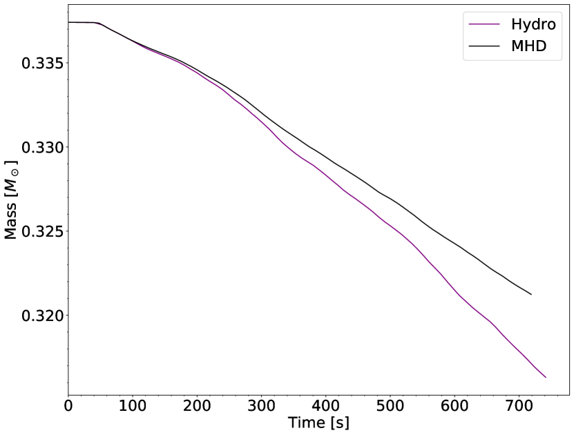
Figure 9: Total mass of neon in the entire computational domain for the purely hydrodynamic simulation (purple) and the MHD simulation (black).

4 Conclusions

We investigated the amplification and saturation of magnetic fields during convective oxygen shell burning and the backreaction of the field on the convective flow by conducting a 3D MHD simulation and a purely hydrodynamic simulation of an $18\,M_{\odot}$ progenitor shortly before core collapse. The simulations were run for about 12 minutes of physical time (corresponding to about 17 convective turnover times), at which point field amplification has slowed down considerably, though a quasi-stationary state has not yet been fully established.

The magnetic field in the oxygen shell is amplified to $\mathord{\sim}10^{10}\,\mathrm{G}$ and dominated by small-to-medium-scale structures with angular wavenumber $\ell\sim 7$. The dipole component is considerably smaller with $\mathord{\sim}10^{9}\,\mathrm{G}$ near the inner boundary of the oxygen shell and less further outside. The profiles of the radial and non-radial diagonal components $M_{rr}$ and $M_{\theta\theta}+M_{\varphi\varphi}$ of the Maxwell stress tensor mirror the corresponding components $R_{rr}$ and $R_{\theta\theta}+R_{\varphi\varphi}$ of the Reynolds stress tensor, but remain about an order of magnitude smaller, i.e., kinetic equipartition is not reached. However, $M_{\theta\theta}+M_{\varphi\varphi}$ can approach or exceed the radial component $R_{rr}$ at the convective boundaries. The saturation mechanism for field amplification needs to be studied in more detail, but we speculate that saturation is mediated by the inhibiting effect of non-radial magnetic fields on shear instabilities at shell boundaries, which appear to be the primary driver of field amplification.

We find that magnetic fields do not have an appreciable effect on the interior flow inside the oxygen shell, but observe a moderate reduction of turbulent entrainment at the oxygen-neon shell boundary in the presence of magnetic fields. Magnetic fields appear to suppress stronger episodic entrainment events, although they do not quench entrainment completely. Through the reduced entrainment rate, magnetic fields also indirectly affect the dynamics inside the convective region slightly because they reduce the energy release through the dissociation of ingested neon, which results in slightly smaller convective velocities in the MHD model.

Our findings have important implications for core-collapse supernova modelling. We predict initial fields in the oxygen shell of non-rotating progenitors that are significantly stronger than assumed in our recent simulation of a neutrino-driven explosion aided by dynamo-generated magnetic fields (Müller & Varma, 2020). With relatively strong seed-fields, there is likely less of a delay until magnetic fields can contribute the additional “boost” to neutrino heating and purely hydrodynamic instabilities seen in Müller & Varma (2020). This should further contribute to the robustness of the neutrino-driven mechanism for non-rotating and slowly-rotating massive stars. Our simulations also suggest that the perturbation-aided mechanism (Couch & Ott, 2013; Müller & Janka, 2015) will not be substantially affected by the inclusion of magnetic fields. Since magnetic fields do not become strong enough to substantially alter the bulk flow inside the convective region, the convective velocities and eddy scales as the key parameters for perturbation-aided explosions remain largely unchanged.

The implications of our results for neutron star magnetic fields are more difficult to evaluate since the observable fields will, to a large degree, be set by processes during and after the supernova and cannot be simply extrapolated from the progenitor stage by magnetic flux conservation. That said, dipole fields of order $10^{9}\,\mathrm{G}$ at the base of the oxygen shell – which is likely to end up as the neutron star surface region – are not in overt conflict with dipole fields of order $10^{13}\,\mathrm{G}$ in many young pulsars inside supernova remnants (Enoto et al., 2019). However, considering the relatively strong small-scale fields of $\mathord{\sim}10^{10}\,\mathrm{G}$ with peak values over $10^{11}\,\mathrm{G}$, it may prove difficult to produce neutron stars without strong small-scale fields at the surface. There is a clear need for an integrated approach towards the evolution of magnetic fields from the progenitor phase through the supernova and into the compact remnant phase in order to fully grasp the implications of the current simulations.

Evidently, further follow-up studies are also needed on the final evolutionary phases of supernova progenitors. Longer simulations and resolution studies will be required to better address issues like the saturation field strength, the saturation mechanism, and the impact of magnetic fields on turbulent entrainment. Full models that include the core and self-consistently follow the evolution of the star to collapse will be required to generate accurate 3D initial conditions for supernova simulations. The critical issue of non-ideal effects and the behaviour of turbulent magnetoconvection for magnetic Prandtl numbers slightly smaller than one at very high Reynolds numbers deserves particular consideration. Some findings of our “optimistic” approach based on the ideal MHD approximation should, however, prove robust, such as the modest effect of magnetic fields on the convective bulk flow and hence the reliability of purely hydrodynamic models (Couch et al., 2015; Müller et al., 2016; Yadav et al., 2020; Müller, 2020; Fields & Couch, 2020) and even 1D mixing-length theory (Collins et al., 2018) to predict pre-collapse perturbations in supernova progenitors. Future 3D simulations will also have to address rotation and its interplay with convection and magnetic fields.

Data Availability

The data underlying this article will be shared on reasonable request to the authors, subject to considerations of intellectual property law.

Appendix A Energy-conserving formulation of hyperbolic divergence cleaning

The original extended generalised Lagrange multiplier formulation of the MHD equations of Dedner et al. (2002) reads (without non-adiabatic energy source/sink terms and the advection equations for the mass fractions),

$$\partial_{t}\rho+\nabla\cdot\rho\mathbf{v} = 0,$$ (13)

$$\partial_{t}(\rho\mathbf{v})+\nabla\cdot\left(\rho\mathbf{v}\mathbf{v}-\frac{\mathbf{B}\mathbf{B}}{4\pi}+P_{\mathrm{t}}\mathcal{I}\right) = \rho\mathbf{g}-\frac{(\nabla\cdot\mathbf{B})\mathbf{B}}{4\pi},$$ (14)

$$\partial_{t}e+\nabla\cdot\left[(e+P_{\mathrm{t}})\mathbf{u}-\frac{\mathbf{B}(\mathbf{v}\cdot\mathbf{B})}{4\pi}\right] = \rho\mathbf{g}\cdot\mathbf{v}-\frac{\mathbf{B}\cdot\nabla\psi}{4\pi},$$ (15)

$$\partial_{t}\mathbf{B}+\nabla\cdot(\mathbf{v}\mathbf{B}-\mathbf{B}\mathbf{v})+\nabla{\psi} = 0,$$ (16)

$$\partial_{t}{\psi}+c_{\mathrm{h}}^{2}\nabla\cdot\mathbf{B} = -{\psi}/\tau.$$ (17)

where $e=\rho\left(\epsilon+v^{2}/2\right)+B^{2}/(8\pi)$ is the standard expression for the total internal, kinetic, and magnetic energy of the fluid. This system includes an extra source term $-\mathbf{B}\cdot\nabla\psi/(4\pi)$ in the energy equation. To ensure total energy conservation, one must also take into account the energy carried by the cleaning field $\psi$, which can be worked out as $e_{\psi}=\psi^{2}/(8\pi c_{\mathrm{h}}^{2})$ (Tricco & Price, 2012). Tricco et al. (2016) noted that that the original system of equations (13–17) of Dedner et al. (2002) no longer guarantees total energy conservation if a variable cleaning speed is used. They show that total energy conservation is recovered if one introduces a rescaled cleaning field $\hat{\psi}=\psi/c_{\mathrm{h}}$ and solves a slightly modified system of equations,

$$\partial_{t}\rho+\nabla\cdot\rho\mathbf{v} = 0,$$ (18)

$$\partial_{t}(\rho\mathbf{v})+\nabla\cdot\left(\rho\mathbf{v}\mathbf{v}-\frac{\mathbf{B}\mathbf{B}}{4\pi}+P_{\mathrm{t}}\mathcal{I}\right) = \rho\mathbf{g}-\frac{(\nabla\cdot\mathbf{B})\mathbf{B}}{4\pi},$$ (19)

$$\partial_{t}e+\nabla\cdot\left[(e+P_{\mathrm{t}})\mathbf{u}-\frac{\mathbf{B}(\mathbf{v}\cdot\mathbf{B})}{4\pi}\right] = \rho\mathbf{g}\cdot\mathbf{v}-\frac{\mathbf{B}\cdot\nabla(c_{\mathrm{h}}\hat{\psi})}{4\pi},$$ (20)

$$\partial_{t}\mathbf{B}+\nabla\cdot(\mathbf{v}\mathbf{B}-\mathbf{B}\mathbf{v})+\nabla(c_{\mathrm{h}}\hat{\psi}), = 0,$$ (21)

$$\partial_{t}\hat{\psi}+c_{\mathrm{h}}\nabla\cdot\mathbf{B} = -\hat{\psi}/\tau,$$ (22)

It is evident that rescaling the cleaning field does not alter the characteristic structure of the system, but the more symmetric formulation of Equations (21) and (22) with identical dimensions for $\hat{\psi}$ and $\mathbf{B}$ allows us to explicitly cast the energy equation in conservation form. The term $c_{\mathrm{h}}\nabla\cdot\mathbf{B}$ in Equation (22) gives a contribution (denoted by a subscript “h”) to the time derivative of the energy associated with the cleaning field,

$$\left(\frac{\partial(\hat{\psi}^{2}/2)}{\partial t}\right)_{\mathrm{h}}=-c_{\mathrm{h}}\hat{\psi}\nabla\cdot\mathbf{B}.$$ (23)

Because of the rescaling of the cleaning field, no time derivative of the cleaning speed $c_{\mathrm{h}}$ appears, which is critical for writing the energy equation in a manifestly conservative form. Adding Equations (20) and (23) yields

$$\partial_{t}\hat{e}+\nabla\cdot\left[(e+P_{\mathrm{t}})\mathbf{u}-\frac{\mathbf{B}(\mathbf{v}\cdot\mathbf{B})}{4\pi}\right]=\rho\mathbf{g}\cdot\mathbf{v}-\frac{\mathbf{B}\cdot\nabla(c_{\mathrm{h}}\hat{\psi})+c_{\mathrm{h}}\hat{\psi}\nabla\cdot\mathbf{B}}{4\pi},$$ (24)

where $\hat{e}=\rho(\epsilon+v^{2}/2)+(B^{2}+\hat{\psi}^{2})/(8\pi)$. The cleaning terms on the right-hand side can be written as a divergence and hence absorbed in the energy flux,

$$\partial_{t}\hat{e}+\nabla\cdot\left[(e+P_{\mathrm{t}})\mathbf{u}-\frac{\mathbf{B}(\mathbf{v}\cdot\mathbf{B})-c_{\mathrm{h}}\hat{\psi}\mathbf{B}}{4\pi}\right]=\rho\mathbf{g}\cdot\mathbf{v}.$$ (25)

As noted by Tricco et al. (2016), the damping term for the cleaning field will effectively add to dissipation into thermal energy in such an approach, but they found the additional dissipation insignificant in practice compared to other sources of numerical dissipation.

black

References

- Abdikamalov & Foglizzo (2020) Abdikamalov E., Foglizzo T., 2020, MNRAS, 493, 3496
- Aguilera-Dena et al. (2018) Aguilera-Dena D. R., Langer N., Moriya T. J., Schootemeijer A., 2018, ApJ, 858, 115
- Aguilera-Dena et al. (2020) Aguilera-Dena D. R., Langer N., Antoniadis J., Müller B., 2020, ApJ, 901, 114
- Aguilera et al. (2008) Aguilera D. N., Pons J. A., Miralles J. A., 2008, A&A, 486, 255
- Akiyama et al. (2003) Akiyama S., Wheeler J. C., Meier D. L., Lichtenstadt I. Meier D. L., Lichtenstadt 2003, ApJ, 584, 954
- Aloy & Obergaulinger (2020) Aloy M.-Á., Obergaulinger M., 2020, Monthly Notices of the Royal Astronomical Society, 500, 4365
- Arnett & Meakin (2010) Arnett W. D., Meakin C., 2010, in Cunha K., Spite M., Barbuy B., eds, IAU Symposium Vol. 265, Chemical Abundances in the Universe: Connecting First Stars to Planets. pp 106–110, doi:10.1017/S174392131000030X
- Arnett et al. (2009) Arnett D., Meakin C., Young P. A., 2009, ApJ, 690, 1715
- Balbus & Hawley (1991) Balbus S. A., Hawley J. F., 1991, ApJ, 376, 214
- Bazan & Arnett (1994) Bazan G., Arnett D., 1994, ApJ, 433, L41
- Bazán & Arnett (1997) Bazán G., Arnett D., 1997, Nuclear Phys. A, 621, 607
- Beresnyak (2019) Beresnyak A., 2019, Living Reviews in Computational Astrophysics, 5, 2
- Biermann (1932) Biermann L., 1932, Z. Astrophys., 5, 117
- Blondin et al. (2003) Blondin J. M., Mezzacappa A., DeMarino C., 2003, ApJ, 584, 971
- Böhm-Vitense (1958) Böhm-Vitense E., 1958, Z. Astrophys., 46, 108
- Bollig et al. (2017) Bollig R., Janka H.-T., Lohs A., Martínez-Pinedo G., Horowitz C. J., Melson T., 2017, Physical Review Letters, 119, 242702
- Bollig et al. (2020) Bollig R., Yadav N., Kresse D., Janka H. T., Mueller B., Heger A., 2020, arXiv e-prints, arXiv:2010.10506
- Brandenburg (2011) Brandenburg A., 2011, ApJ, 741, 92
- Bugli et al. (2020) Bugli M., Guilet J., Obergaulinger M., Cerdá-Durán P., Aloy M. A., 2020, MNRAS, 492, 58
- Burrows et al. (1995) Burrows A., Hayes J., Fryxell B. A., 1995, ApJ, 450, 830
- Burrows et al. (2007) Burrows A., Dessart L., Livne E., Ott C. D., Murphy J., 2007, ApJ, 664, 416
- Burrows et al. (2018) Burrows A., Vartanyan D., Dolence J. C., Skinner M. A., Radice D., 2018, Space Science Reviews, 214, 33
- Burrows et al. (2019) Burrows A., Radice D., Vartanyan D., 2019, MNRAS, 485, 3153
- Burrows et al. (2020) Burrows A., Radice D., Vartanyan D., Nagakura H., Skinner M. A., Dolence J. C., 2020, MNRAS, 491, 2715
- Cantiello et al. (2007) Cantiello M., Yoon S. C., Langer N., Livio M., 2007, A&A, 465, L29
- Chandrasekhar (1961) Chandrasekhar S., 1961, Hydrodynamic and Hydromagnetic Stability. Clarendon, Oxford
- Charbonneau (2014) Charbonneau P., 2014, ARA&A, 52, 251
- Chatzopoulos et al. (2016) Chatzopoulos E., Couch S. M., Arnett W. D., Timmes F. X., 2016, ApJ, 822, 61
- Christensen et al. (2009) Christensen U. R., Holzwarth V., Reiners A., 2009, Nature, 457, 167
- Collins et al. (2018) Collins C., Müller B., Heger A., 2018, MNRAS, 473, 1695
- Couch & Ott (2013) Couch S. M., Ott C. D., 2013, ApJ, 778, L7
- Couch et al. (2015) Couch S. M., Chatzopoulos E., Arnett W. D., Timmes F. X., 2015, ApJ, 808, L21
- Cristini et al. (2017) Cristini A., Meakin C., Hirschi R., Arnett D., Georgy C., Viallet M., Walkington I., 2017, MNRAS, 471, 279
- Cristini et al. (2019) Cristini A., Hirschi R., Meakin C., Arnett D., Georgy C., Walkington I., 2019, MNRAS, 484, 4645
- De Grandis et al. (2020) De Grandis D., Turolla R., Wood T. S., Zane S., Taverna R., Gourgouliatos K. N., 2020, ApJ, 903, 40
- Dedner et al. (2002) Dedner A., Kemm F., Kröner D., Munz C. D., Schnitzer T., Wesenberg M., 2002, Journal of Computational Physics, 175, 645
- Duncan & Thompson (1992) Duncan R. C., Thompson C., 1992, ApJ, 392, L9
- Endeve et al. (2012) Endeve E., Cardall C. Y., Budiardja R. D., Beck S. W., Bejnood A., Toedte R. J., Mezzacappa A., Blondin J. M., 2012, ApJ, 751, 26
- Enoto et al. (2019) Enoto T., Kisaka S., Shibata S., 2019, Reports on Progress in Physics, 82, 106901
- Federrath et al. (2011) Federrath C., Chabrier G., Schober J., Banerjee R., Klessen R. S., Schleicher D. R. G., 2011, Phys. Rev. Lett., 107, 114504
- Fejer (1964) Fejer J. A., 1964, Physics of Fluids, 7, 499
- Fernando (1991) Fernando H. J. S., 1991, Annual Review of Fluid Mechanics, 23, 455
- Ferrario & Wickramasinghe (2005) Ferrario L., Wickramasinghe D. T., 2005, MNRAS, 356, 615
- Ferrario et al. (2009) Ferrario L., Pringle J. E., Tout C. A., Wickramasinghe D. T., 2009, MNRAS, 400, L71
- Ferrario et al. (2015) Ferrario L., de Martino D., Gänsicke B. T., 2015, Space Sci. Rev., 191, 111
- Fields & Couch (2020) Fields C. E., Couch S. M., 2020, ApJ, 901, 33
- Foglizzo et al. (2007) Foglizzo T., Galletti P., Scheck L., Janka H.-T., 2007, ApJ, 654, 1006
- Frank et al. (1996) Frank A., Jones T. W., Ryu D., Gaalaas J. B., 1996, ApJ, 460, 777
- Fuller et al. (2019) Fuller J., Piro A. L., Jermyn A. S., 2019, MNRAS, 485, 3661
- Grinstein et al. (2007) Grinstein F., Margolin L., Rider W., 2007, Implicit Large Eddy Simulation - Computing Turbulent Fluid Dynamics. Cambridge University Press
- Gurski (2004) Gurski K. F., 2004, SIAM Journal on Scientific Computing, 25, 2165
- Heger & Woosley (2010) Heger A., Woosley S. E., 2010, Astrophysical Journal, 724, 341
- Heger et al. (2005) Heger A., Woosley S. E., Spruit H. C., 2005, ApJ, 626, 350
- Herant et al. (1994) Herant M., Benz W., Hix W. R., Fryer C. L., Colgate S. A., 1994, ApJ, 435, 339
- Horowitz et al. (2017) Horowitz C. J., Caballero O. L., Lin Z., O’Connor E., Schwenk A., 2017, Phys. Rev. C, 95, 025801
- Hotta et al. (2015) Hotta H., Rempel M., Yokoyama T., 2015, ApJ, 803, 42
- Iskakov et al. (2007) Iskakov A. B., Schekochihin A. A., Cowley S. C., McWilliams J. C., Proctor M. R. E., 2007, Phys. Rev. Lett., 98, 208501
- Janka & Müller (1995) Janka H.-T., Müller E., 1995, ApJ, 448, L109
- Janka & Müller (1996) Janka H.-T., Müller E., 1996, A&A, 306, 167
- Jones et al. (2017) Jones S., Andrassy R., Sandalski S., Davis A., Woodward P., Herwig F., 2017, MNRAS, 465, 2991
- Käpylä et al. (2020) Käpylä P. J., Gent F. A., Olspert N., Käpylä M. J., Brandenburg A., 2020, Geophys. Astrophys. Fluid Dyn., 114, 8
- Kaspi & Beloborodov (2017) Kaspi V. M., Beloborodov A. M., 2017, ARA&A, 55, 261
- Keppens et al. (1999) Keppens R., Tóth G., Westermann R. H. J., Goedbloed J. P., 1999, Journal of Plasma Physics, 61, 1
- Kuhlen et al. (2003) Kuhlen M., Woosley W. E., Glatzmaier G. A., 2003, in Turcotte S., Keller S. C., Cavallo R. M., eds, Astronomical Society of the Pacific Conference Series Vol. 293, 3D Stellar Evolution. p. 147
- Kuroda et al. (2020) Kuroda T., Arcones A., Takiwaki T., Kotake K., 2020, ApJ, 896, 102
- Lentz et al. (2015) Lentz E. J., et al., 2015, ApJ, 807, L31
- Liu et al. (2018) Liu Y., Chen Z. H., Zhang H. H., Lin Z. Y., 2018, Physics of Fluids, 30, 044102
- McNeill & Müller (2020) McNeill L. O., Müller B., 2020, MNRAS, 497, 4644
- Meakin & Arnett (2006) Meakin C. A., Arnett D., 2006, ApJ, 637, L53
- Meakin & Arnett (2007a) Meakin C. A., Arnett D., 2007a, ApJ, 665, 690
- Meakin & Arnett (2007b) Meakin C. A., Arnett D., 2007b, ApJ, 667, 448
- Melson et al. (2015) Melson T., Janka H.-T., Bollig R., Hanke F., Marek A., Müller B., 2015, ApJ, 808, L42
- Miura & Pritchett (1982) Miura A., Pritchett P. L., 1982, J. Geophys. Res., 87, 7431
- Miyoshi & Kusano (2005) Miyoshi T., Kusano K., 2005, Journal of Computational Physics, 208, 315
- Mocák et al. (2018) Mocák M., Meakin C., Campbell S. W., Arnett W. D., 2018, Monthly Notices of the Royal Astronomical Society, 481, 2918
- Monchaux et al. (2007) Monchaux R., et al., 2007, Phys. Rev. Lett., 98, 044502
- Mösta et al. (2014) Mösta P., et al., 2014, Astrophysical Journal Letters, 785, 29
- Mösta et al. (2018) Mösta P., Roberts L. F., Halevi G., Ott C. D., Lippuner J., Haas R., Schnetter E., 2018, ApJ, 864, 171
- Müller (2016) Müller B., 2016, Publ. Astron. Soc. Australia, 33, e048
- Müller (2020) Müller B., 2020, Living Reviews in Computational Astrophysics, 6, 3
- Müller & Janka (2015) Müller B., Janka H.-T., 2015, MNRAS, 448, 2141
- Müller & Varma (2020) Müller B., Varma V., 2020, MNRAS, 498, L109
- Müller et al. (2016) Müller B., Viallet M., Heger A., Janka H.-T., 2016, ApJ, 833, 124
- Müller et al. (2017) Müller B., Melson T., Heger A., Janka H.-T., 2017, MNRAS, 472, 491
- Müller et al. (2019) Müller B., et al., 2019, MNRAS, 484, 3307
- Obergaulinger & Aloy (2020a) Obergaulinger M., Aloy M.-Á., 2020a, MNRAS, 492, 4613
- Obergaulinger & Aloy (2020b) Obergaulinger M., Aloy M.-Á., 2020b, arXiv e-prints, arXiv:2008.07205
- Obergaulinger, M. et al. (2010) Obergaulinger, M. Aloy, M. A. Müller, E. 2010, A&A, 515, A30
- Obergaulinger et al. (2014) Obergaulinger M., Janka H.-T., Aloy M. A., 2014, MNRAS, 445, 3169
- Olausen & Kaspi (2014) Olausen S. A., Kaspi V. M., 2014, ApJS, 212, 6
- Pétrélis et al. (2007) Pétrélis F., Mordant N., Fauve S., 2007, Geophysical and Astrophysical Fluid Dynamics, 101, 289
- Pietarila Graham et al. (2010) Pietarila Graham J., Cameron R., Schüssler M., 2010, ApJ, 714, 1606
- Powell & Müller (2020) Powell J., Müller B., 2020, MNRAS, 494, 4665
- Raynaud et al. (2020) Raynaud R., Guilet J., Janka H.-T., Gastine T., 2020, Science Advances, 6, eaay2732
- Rembiasz et al. (2017) Rembiasz T., Obergaulinger M., Cerdá-Durán P., Aloy M.-Á., Müller E., 2017, ApJS, 230, 18
- Rempel (2014) Rempel M., 2014, Astrophysical Journal, 789, 132
- Ryu et al. (2000) Ryu D., Jones T. W., Frank A., 2000, ApJ, 545, 475
- Sahoo et al. (2011) Sahoo G., Perlekar P., Pandit R., 2011, New Journal of Physics, 13, 013036
- Schekochihin et al. (2004) Schekochihin A. A., Cowley S. C., Maron J. L., McWilliams J. C., 2004, Phys. Rev. Lett., 92, 054502
- Schekochihin et al. (2007) Schekochihin A. A., Iskakov A. B., Cowley S. C., McWilliams J. C., Proctor M. R. E., Yousef T. A., 2007, New Journal of Physics, 9, 300
- Schneider et al. (2020) Schneider F. R. N., Ohlmann S. T., Podsiadlowski P., Röpke F. K., Balbus S. A., Pakmor R., 2020, MNRAS, 495, 2796
- Sen (1963) Sen A. K., 1963, Physics of Fluids, 6, 1154
- Seshasayanan et al. (2017) Seshasayanan K., Gallet B., Alexakis A., 2017, Phys. Rev. Lett., 119, 204503
- Spruit (2002) Spruit H. C., 2002, A&A, 381, 923
- Strang & Fernando (2001) Strang E. J., Fernando H. J. S., 2001, Journal of Fluid Mechanics, 428, 349
- Takahashi & Langer (2020) Takahashi K., Langer N., 2020, arXiv e-prints, arXiv:2010.13909
- Takahashi & Yamada (2014) Takahashi K., Yamada S., 2014, ApJ, 794, 162
- Takahashi et al. (2016) Takahashi K., Iwakami W., Yamamoto Y., Yamada S., 2016, ApJ, 831, 75
- Takiwaki et al. (2014) Takiwaki T., Kotake K., Suwa Y., 2014, ApJ, 786, 83
- Tauris et al. (2015) Tauris T. M., et al., 2015, in Advancing Astrophysics with the Square Kilometre Array (AASKA14). p. 39 (arXiv:1501.00005)
- Thaler & Spruit (2015) Thaler I., Spruit H. C., 2015, A&A, 578, A54
- Thelen & Cattaneo (2000) Thelen J. C., Cattaneo F., 2000, MNRAS, 315, 13
- Thompson & Duncan (1993) Thompson C., Duncan R. C., 1993, ApJ, 408, 194
- Torres-Forné et al. (2016) Torres-Forné A., Cerdá-Durán P., Pons J. A., Font J. A., 2016, MNRAS, 456, 3813
- Tricco & Price (2012) Tricco T. S., Price D. J., 2012, Journal of Computational Physics, 231, 7214
- Tricco et al. (2016) Tricco T. S., Price D. J., Bate M. R., 2016, Journal of Computational Physics, 322, 326
- Viganò et al. (2013) Viganò D., Rea N., Pons J. A., Perna R., Aguilera D. N., Miralles J. A., 2013, MNRAS, 434, 123
- Weaver et al. (1978) Weaver T. A., Zimmerman G. B., Woosley S. E., 1978, ApJ, 225, 1021
- Winteler et al. (2012) Winteler C., Käppeli R., Perego A., Arcones A., Vasset N., Nishimura N., Liebendörfer M., Thielemann F. K., 2012, Astrophysical Journal Letters, 750, 22
- Woosley & Heger (2006) Woosley S. E., Heger A., 2006, ApJ, 637, 914
- Woosley et al. (2002) Woosley S. E., Heger A., Weaver T. A., 2002, Rev. Mod. Phys., 74, 1015
- Yadav et al. (2020) Yadav N., Müller B., Janka H. T., Melson T., Heger A., 2020, ApJ, 890, 94
- Yasin et al. (2020) Yasin H., Schäfer S., Arcones A., Schwenk A., 2020, Phys. Rev. Lett., 124, 092701
- Yoon & Langer (2005) Yoon S. C., Langer N., 2005, A&A, 443, 643
- Yoon et al. (2010) Yoon S. C., Woosley S. E., Langer N., 2010, ApJ, 725, 940
- Yoshida et al. (2019) Yoshida T., Takiwaki T., Kotake K., Takahashi K., Nakamura K., Umeda H., 2019, ApJ, 881, 16
- Yoshida et al. (2020) Yoshida T., Takiwaki T., Kotake K., Takahashi K., Nakamura K., Umeda H., 2020, arXiv e-prints, arXiv:2012.13261