Long-Term Autonomy in Forest Environment using Self-Corrective SLAM

Abstract

Vehicles with prolonged autonomous missions have to maintain environment awareness by simultaneous localization and mapping (SLAM). Closed loop correction is substituted by interpolation in rigid body transformation space in order to systematically reduce the accumulated error over different scales. The computation is divided to an edge computed lightweight SLAM and iterative corrections in the cloud environment. Tree locations in the forest environment are sent via a potentially limited communication bandwidths. Data from a real forest site is used in the verification of the proposed algorithm. The algorithm adds new iterative closest point (ICP) cases to the initial SLAM and measures the resulting map quality by the mean of the root mean squared error (RMSE) of individual tree clusters. Adding 4 % more match cases yields the mean RMSE 0.15 m on a large site with 180 m odometric distance.

1 Introduction

The past decade has seen a rapid evolution of methods and technologies in onboard odometry for autonomous navigation and localization. The state-of-the-art has reached a significant level of maturity in both lidar-based shan2018lego and visual-based odometry, among others qin2018vins . Nonetheless, drift in long-term operation is an inherent problem to methods based only on on-board sensors and data, with the probability of a lost position estimation increasing over time queralta2020viouwb . Most methods address this with loop closure shan2018lego ; qin2018vins , where data is compared with older records if locations are repeated. In any case, long-term autonomy based only on onboard odometry data still presents significant challenges. In remote and unstructured environments such as forests, typical methods do not always apply, and loop closure can rarely be applied li2020a . In these scenarios, onboard processing at the edge without network-based computational offloading has inherent limitations. Challenges arise from the point of view of memory (amount of scan data to be stored for later processing), from the perspective of computational load and latency (amount of data to be used for localization through point cloud matching processes), and in terms of the update rate of the localization process (how often is the relative position computed).

Specifically, this paper deals with the problem of Simultaneous Localization and Mapping (SLAM) in unstructured forest environments with 3D laser scanners. SLAM algorithms aim at tracking the movement of the laser scanner (odometry) related to its surroundings and creating a composition from individual views, which consist of scanned point clouds (PC), and scanner positions and orientations. A laser scanner attached to a vehicle provides a spatial input signal which can be a very powerful component in supporting situational awareness, especially when fused with input of other sensors.

A structure from motion (SfM) study engel2018 divides SLAM methods by two divisions: indirect and direct methods, and sparse and dense approaches. One can add three more divisions: probabilistic and non-probabilistic methods, structured and non-structured environments li2020a , and fixed and adaptive frame sampling. Indirect methods rely on early frame-by-frame processing, which produces a set of anchor points. The fixed frame sampling uses every frame or a fixed ratio of frames, whereas adaptive sampling tends to skip a sequence of highly similar frames. The case chosen here uses indirect anchor points from adaptively chosen frames, is non-probabilistic and is aimed to a forest environment, which is non-structured and has nearly uniformly distributed sparse anchor PC.

State of the art: Iterative closest points (ICP) is the standard baseline method in SLAM. It is the computationally most economic choice in its simplest versions, if the convergence can be guaranteed by the application specifics. If a PC is near-uniformly random, the overlap ratio of visible cones is a good estimation for an outlier ratio $\gamma$, which is one of the few tuning parameters used by robust ICPs chetverikov2002 . The outlier ratio $\gamma$ limits the ICP matching process to $1-\gamma$ part of the match pairs and reduces the accumulation of the odometric error. If the matches occur in a geometrically consistent zone between two PCs, the match overlap ratio $\lambda$ can be estimated by $\lambda\approx 1-\gamma$.

The strategy of forcing a minimum overlap does not guarantee global convergence, though. A globally optimal method with a proven convergence is Go-ICP yang2015 , which can detect a difference between a local and global ICP match in the case of near-uniform PC. Other ’global’ methods try to smooth the mean matching error, which is the target function, by various means, but fail to guarantee the convergence to a global optimum.

Near uniform randomness gives a chance to tighten the conditions of branch-and-bound (BnB) limit estimates used in yang2015 . We use Go-ICP as a backbone of a naive and risky SLAM method pcregistericp() matlab2020 since there are no SLAM methods specifically suited for sparse uniformly random PCs to the best of our knowledge.

When dealing with a limited view cone (less than 360^o view), a problem similar to closed loop detection williams2009 ; wang2019 occurs each time the view cone coincides with a much older frame. This happens in a small scale of 2 to 5 m but it can also happen over distances of 0.5 km to 1 km.

Motivation: Autonomous mobile robots and specifically unmanned aerial vehicles (UAVs) have seen an increase penetration for forest surveying and remote sensing chisholm2013uav ; sankey2017uav . Owing to the unstructured environments that forests represent, autonomous navigation presents inherent challenges. Key issues appear in the areas of localization and mapping, where one has to take into account several key points in a local scope to make the SLAM computationally feasible li2020a . Moreover, an autonomy stack for forest navigation ought to consider long-term autonomy (e.g., owing to the long distances that UAVs can traverse over long times, or the longer time that ground vehicles can operate). Typical odometry techniques relying on loop closure do not suffice because locations are not repeated often. In particular, we are interested in lidar-based odometry, localization and mapping with methods that can be used for both unmanned ground vehicles (UGVs) and UAVs.

Taking into account these considerations, there is a need for more advanced techniques for long-term autonomy exploiting registrations of the same objects even from distant locations. This approach differs from traditional loop closure as there can be several partial overlaps of frames over different time scales, and the partial overlap may occur over large distances. Modern laser scanners, even low-cost solid state LiDARs, are capable of measuring distance to objects up to several hundreds of meters ortiz2019initial .

In addition to the accuracy of localization over long distances, the majority of the state-of-the-art lidar-based SLAM algorithms require relatively high computational resources to operate in real-time shan2018lego ; lin2020loam . Moreover, the amount of points in a single scan PC have increased to millions per second in recent years. Solid state lidars with limited field of view (FoV) are only able to detect a reduced number of features in a single scan, but the scan density increases significantly. Therefore, techniques that need to compare all points (e.g., ICP) or traditional feature extraction techniques do not scale well. From the perspective of map-based localization, a similar issue arises with approaches such as the normal distribution transform (NDT)  einhorn2015generic .

Our approach extends the idea of loop closure to track features (i.e., tree stems) over long-term autonomous operation, which can be stored and compared in the form of sparse PCs. Relying in sparse PCs that contain only uniformly distributed features, we are able to both reduce the processing time for localization (in terms of point cloud matching) and the size in memory of larger-scale maps.

In general, we see a gap in the literature in approaches to long-term autonomy and self-corrective localization leveraging the matching of uniformly random feature points. To the best of our knowledge, this together with exploiting sparse PCs for faster processing in unstructured environments has not been addressed yet. Moreover, our approach can be leveraged for managing and accounting for the actively rotating view cone of modern solid-state lidars.

Recently, there have been progress in rigid body interpolation lynch2017 mainly applied in the robotics field. There is an advantage in having both rotation and translation addressed at the same time. To our understanding, this provides a chance to address the odometric consistency independently of the scale of the localization problem.

Contribution:

We propose a method to reduce the cumulative match error by adding extra ICP matches, which comprise a large time interval. Frames within the interval are squeezed together by an interpolation scheme reducing the imprint of sets of anchor points associated together in the final map. The process reduces the noise and blur in the final map, increases the odometric accuracy and solves both small scale closed loop occurrences due to the work cycle movements, and large scale closed loop problems.

In summary, in this paper we address the following three issues: (i) a self-corrective localization algorithm able to incrementally increase the accuracy of the produced environment map without relying on loop closure; (ii) memory efficiency and computation at the edge by relying on sparse point clouds and long-term tracking of features; and (iii) an adaptive approach that adjusts the positioning update rate based on the available data at a given time.

2 Methods

The site and the data: The test data is from a forest operation site in Pankakangas at Lieksa, Eastern Finland (63^o 19.08’ N, 30^o 11.57’ E). The data was recorded on August 2017 in co-operation with participants enlisted in the Acknowledgements section. The sample has a strip road of length 130 m. There are 9009 data frames and 3.7 GB of .pcap data. The total number of trees is 680 and one frame includes 130 trees on the average. An example scanner view is depicted in the left detail of Fig. 1. The mean distance to nearest trees is $L_{0}=3.5$ m excluding the peripheral zone at a distance of 40 m. The right detail shows how the mean distance increases over the radial distance.

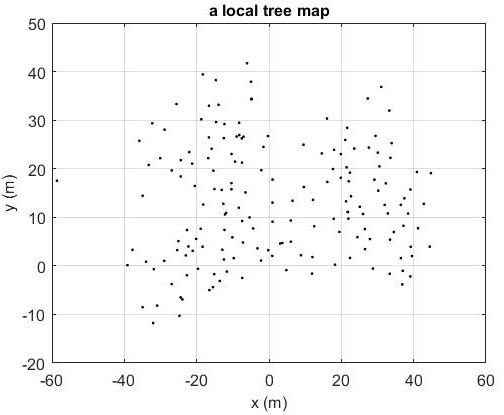
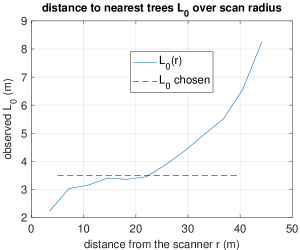
Figure 1: Left: A single scanner view. Each point represents an edge-computed registration of a tree. Points are 3D even shown in a horizontal projection. Right: Mean distances to nearest trees at each scanner range. $L_{0}=3.5$ m is over all the trees and is depicted with a dash line.

Methodology: A simple and fast ICP method pcregistericp() chen1992 ; besl1992 implemented in Matlab matlab2020 produces rigid body transformations, which can be used to build an environment map from sparse key points, each key point representing a detected tree in a scanner view. The problem is to improve this rather low-quality tree map by selecting a small set of promising pairs of frames and producing a computationally more expensive and more accurate match using Go-ICP yang2015 . Each extra match between frames $j$ and $i$ may engulf several frames, which should be properly adapted to the newly introduced and very reliable match. The exponential interpolation of rigid body transformations is used for that purpose.

We introduce first the rigid body transformation as a homogenous operator and its logarithm and exponentiation, which are the core of the interpolation method. A novel aspect is the operator power being in the matrix form. We show that the interpolation is contractive meaning that the final PC map improves (individual tree clusters become sharper) per each addition of extra matches. The sharpening can be measured internally by minimization of the mean match error and externally by observing the mean radius of clusters in the final map. Finally we define the control parameters for the branch-and-bound (BnB) of the global minimum search of the SLAM match.

2.1 Operator exponentiation

A rigid body transformation $\tau\in SE(3)$ in the special Euclidean group $SE(3)$ consists of one rotation represented by a rotation $R\in SO(3)$ within the special orthogonal group $SO(3)$ followed by and a translation $p\in\mathbb{R}^{3}$. The treatise uses the notation and conventions of lynch2017 . The transformation $\tau$ can be seen as a homogenous mapping $\tau:\ q\mapsto q^{\prime}$:

$$\pmatrix{q}^{\prime}\\ 1=\overbrace{\pmatrix{[}R]&p\\ 0\ 1}^{[\tau]}\pmatrix{q}\\ 1,$$ (1)

where braces $[.]$ depict the matrix representation of an operator. Transformation $\tau(R,p)$ is defined by a pair of a rotation and a translation. An alternative parameterization is $\tau(\vec{\omega},\theta,v)$ where a unit axis $\vec{\omega}=(\omega_{1}\,\omega_{2}\,\omega_{3})\in\mathbb{R}^{3}$ is the rotation axis, $\theta$ is a rotation angle around that axis, and $v\in\mathbb{R}^{3}$ is the tangential direction, where the origo moves in the beginning of that rotation. Note that $\vec{\omega}$ is the unit eigenvector of $[R]$ associated to the eigenvalue 1: $[R]\vec{\omega}=\vec{\omega}$.

A twist $S([\omega],v)$ combines two of the elements of a rigid body transformation, and its matrix form is:

$$[S]=\pmatrix{[}\omega]&v\\ 0\ 0,$$ (2)

where $[\omega]a=\vec{\omega}\times a$ for any $a\in\mathbb{R}$, or, as written open in the matrix form:

$$[\omega]=\pmatrix{0}&-\omega_{3}\omega_{2}\\ \omega_{3}0-\omega_{1}\\ -\omega_{2}\omega_{1}0.$$ (3)

Note that this definition gives $[\omega]$ a cyclic property: $[\omega]^{3}=-[\omega]$ which will be used, when dealing with series expansions of $e^{x}$, $\sin{x}$ and $\cos{x}$. Exponentiation of $[S]\theta$ gives us:

$$e^{[S]\theta}=\pmatrix{e}^{[\omega]\theta}&G(\theta)v\\ 0\ 1=[\tau],$$ (4)

where the right equality can be settled by setting $v=G^{-1}(\theta)p$ and $e^{[\omega]\theta}=[R]$. The twist gain function $G(\theta)$ unfolds by the exponentiation series and the rotation matrix term can be expanded to a closed form:

$$[R]=I+\sin{\theta}[\omega]+(1-\cos{\theta})[\omega]^{2},$$ (5)

which is the well-known Rodriguez formula. Finally, raising $\tau$ to a power $u\in\mathbb{R}$, one gets:

$$[\tau^{u}]=\pmatrix{[}R^{u}]&p_{u}\\ 0\ 1,$$ (6)

where

$$[R^{u}] = I+\sin{\theta u}[\omega]+(1-\cos{\theta u})[\omega]^{2}$$ (7)

$$p_{u} = G(\theta u)G^{-1}(\theta)p.$$ (8)

The homogenous representation allowed a definition of a matrix power of a rigid body transformation limited to $SE(3)$. To signify this limitation, we write $[\tau^{u}]$ and not $[\tau]^{u}$, since the wide realm of general matrices is perilous moler2003 , what comes to exponentiation and taking logarithms. The same argument holds to notation with $[R^{u}]$.

The twist gain function $G(\theta)$ is opened next:

$$G(\theta)=I\theta+(1-\cos{\theta})[\omega]+(\theta-\sin{\theta})[\omega]^{2}.$$ (9)

Its inverse is needed in the Equation 8:

$$G^{-1}(\theta)=\frac{1}{\theta}I-\frac{1}{2}[\omega]+\left(\frac{1}{\theta}-\frac{1}{2\tan(\theta/2)}\right)[\omega]^{2}.$$ (10)

One can easily see that there is a singularity in $G^{-1}(\theta)$ when $\theta\rightarrow 0$. But the product in Eq. 8 stays defined, albeit it needs a Taylor series expansion at $\theta=0$. This is needed because the homogenous formulation chosen here is not a conformal theory dorst2009 . The product $G(\theta u)G^{-1}(\theta)$ develops to: G(θu)G^-1(θ)=Iu+[A(θ,u)-sinθu2][ω]+
+[u-1-cosθu2- B(θ,u)][ω]^2, where:

$$A(\theta,u)=\frac{1-\cos{\theta u}}{2\tan{\theta/2}},\;B(\theta,u)=\frac{\sin{\theta u}}{2\tan{\theta/2}},$$ (11)

which are both of a form 0/0 at $\theta=0$. Taylor series developed at $\theta=0$ give:

$$A(\theta,u) =\frac{u^{2}}{2}\theta-(u^{2}+u^{4})\theta^{3}/24+\mathcal{O}(\theta^{4})$$ (12)

$$B(\theta,u) =u-(u/12+u^{3}/6)\theta^{2}+\mathcal{O}(\theta^{4}).$$ (13)

Note that small values of $\theta$ will often occur with the intended application, whereas large values $\theta\approx\pi$ occur seldomlu, if ever.

Extraction of $[\omega]$ and $\theta$ from a given $[R]$ is called taking a rotation logarithm, since $[R]=e^{[\omega]\theta}$. The exact logarithm algorithm is given in lynch2017 and has two special cases for $\theta\approx 0$ and $\theta\approx\pi$. The intended application of the transformation matrix power is such that one needs to solve the Eq. 6 several times with different values of $u$, so the constant parts $[\omega]$ and $\theta$ are pivotal. Fig. 2 shows an example, where a rigid body co-ordinate frame $\tau_{a}$ is interpolated to another frame $\tau_{b}$ using 11 values $u\in[0,1]\mathbb{R}$.

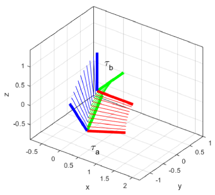
Figure 2: Example of a power interpolation $\tau_{u}=\tau_{a}^{1-u}\tau_{b}^{u}$. When $u=0\rightarrow 1$, $\tau_{u}=\tau_{a}\rightarrow\tau_{b}$ smoothly between two rigid body frames $\tau_{a}$ and $\tau_{b}$. Columns of $[R]$ form the orthogonal frame axes, which are shown in red, green and blue.

The matrix power in Eq. 6 has one special case of pure translation where there is no rotation ($\theta=0$ and $[R]=I$) with:

$$\pmatrix{I}&p\\ 0\ 1^{u}=\pmatrix{I}&pu\\ 0\ 1.$$ (14)

Naturally, this special case should be covered by a general solution of the vector $p_{u}$. As a sanity check, setting $\theta\approx 0$ leads to $p_{u}\approx pu$ for all $u\in\mathbb{R}$. By setting $u=1$ and after a tedious trigonometric manipulation, one gets $p_{u}=p$ for all $\theta$. Although the Eqs. 1- 13 are novel in the context of the matrix power of the homogenous formulation, a similar Taylor series approach has been presented for dual quaternion exponentiation and logarithm in dantam2018 , and one could construct a similar transformation power $\tau^{u}$ using suitable quaternion libraries. The value of the Eqs. 1- 13 is that the odometric process described in the next section can proceed within a usual matrix infrastructure. The computational price tag of two alternative formulations (dual quaternions and homogenous co-ordinates) for taking multiple matrix powers is surprisingly close to each other for large PCs.

A study on the error of the exponentiation of the rigid body transformation follows. Two consecutive operations $\|[(t^{u})^{1/u}]-[t]\|$ produce an error shown in the Fig. 3. The result is the average over 300 rigid body transformations with a uniform distributed $p\in[-1,1]^{3}\subset\mathbb{R}^{3}$ and $R(\vec{\omega},\theta)$, where $\vec{\omega}\in S^{2}$ is uniformly distributed over a unit sphere $S^{2}\subset\mathbb{R}^{3}$ and $\theta\in[0,\pi)$ is also uniformly distributed. The sequential matrix multiplication version with $1/u\in\mathbb{N}$ has been provided (red line) alongside the usual $u\in[0,1]\subset\mathbb{R}$ matrix power test (blue line). As can be seen from the Fig. 3, the computational accuracy is not a problem near $u=0$, and $u\approx 1$ does not usually occur. The overall accuracy in the multiplication case is $4.8\times 10^{-3}$, which is enough for practical implementation. Both tests are clearly conservative when compared to actual computations, which generate new operators $\tau^{u}$ from constant values $\theta$ and $[\omega]$.

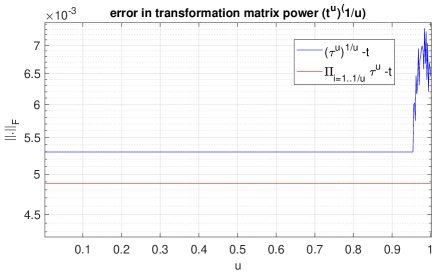
Figure 3: A numerical verification of rising rigid body transformations to a power $u$. Blue line depicts taking a power $u$ and then $1/u$. Red line is for taking a power $u$ followed by a number ($1/u\in\mathbb{N}$) of matrix multiplications.

2.2 Rigid body motion interpolation

This Section expands the presentation in nevalainen2020a and uses the notation of lynch2017 . The detailed definitions are provided since the formulations come from a variety of sources. Odometry is built by matching sequential PCs $P_{l}$ and $P_{l+1}$ in the coordinate system of the frame $l$ by estimating a transformation $\tau_{l+1\,l}$ (from a frame $l+1$ to the frame $l$). A simple and fast ICP method pcregistericp() of Matlab matlab2020 ; chen1992 ; besl1992 is applied to produce a sequence of rigid body transformations $\tau_{l+1\,l}$ from a frame $l+1$ to a frame $l$. This process is not secure, it is possible to have an erroneous match, which is off some 2-10 meters.

The combination of two PCs achieved by a succesful match is denoted by $.\match.$ as: $P_{l}\match P_{l+1}t_{l+1\,l}$, where $t_{ij}=[\tau_{ij}]^{T}$ because, unlike in the definition of Eq 1, points are now columns of a PC matrix. A match between frames $l+1$ and $l$ includes inaccuracies $e_{l}$, and identification of outliers (points not matched to any point) and of matching pairs of points. The final SLAM result has all frames matched to the first frame:

$$P=\match_{l=1}^{n}P_{l}\,t_{l1}$$ (15)

where $n$ is the number of frames, $t_{11}=I$ and total transformation matrices $t_{l1}$ are built iteratively from local matches $t_{l+1\,l}$ by: $t_{l+1\,1}=t_{l1}t_{l+1\,l}$.

The PCs $P_{l}\,t_{l1}$ each contribute to the total map $P$. A typical ICP process produces a chain of stepwise transformations $\tau_{l+1}^{l},\,1\leq l<n$. One can recover a random transformation between frames $i$ and $j$ from total transformations by:

$$t_{ij}={t_{j1}}^{-1}t_{i1}.$$ (16)

The iterative application of the Eq. 15 is called globalization (or SLAM process). The odometry problem is solved when the globalized translation vectors are extracted. The path $Q$ of the vehicle is:

$$Q=\{q_{i1}\,|\,\tau_{i1}=(R_{i1},\,q_{i1})\}_{i=1...n}$$ (17)

The basic scenario of the self-corrrective odometry is depicted in Fig. 4 using two paths $Q$ and $Q^{\prime}$ to represent a situation, where some of the transformations $t_{l+1\,l},\,j\leq l<i$ have been judged inaccurate, noisy or inexact by some criteria. The criteria is usually related to the blurriness of the global map. Then a corrective check is being performed from the frame $j$ to the frame $i$ producing an improvement of a match. Formally, an error measure $e(P_{j}\match P_{i}\,{t_{ij}}^{\prime})<e(P_{j}\match P_{i}\,{t_{ij}})$ of a match improves, when a new match ${t_{ij}}^{\prime}$ is used instead of a synthetized transformation $t_{ij}$ of Eq 16. Now, all the intermediary PCs $PC_{l},\,j<l<i$ need to be updated.

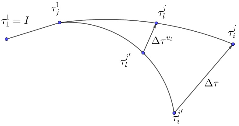
Figure 4: An update from $\tau_{i1}$ to ${\tau_{i1}}^{\prime}$ makes the old path $j+1,...,i-1$ incompatible. It can be corrected by any interpolation scheme, e.g. the Eq. 18.

A solution is to force the differences $\Delta\tau_{l}$ to have boundary conditions $\Delta t_{j}=I$ and $\Delta t_{i}=\Delta t={t_{ij}}^{-1}{t_{ij}}^{\prime}$. A rather obvious interpolator is by $\Delta t_{l}=\Delta t^{u_{l}}$, where $0\leq u_{l}\leq 1$ with obvious end conditions $u_{j}=0,\,u_{i}=1$. Assuming representative powers $u_{l}$ are defined for each transformation $t_{lj},\,j\leq l\leq i$, one can solve new values ${t_{lj}}^{\prime}$:

$$t_{l1}:={t_{l1}}^{\prime}=t_{j1}t_{lj}\Delta t^{u_{l}},$$ (18)

where ’:=’ denotes a computational substitution of a new value. As a sanity test, by setting $l=j,\,u_{l}=0$ one gets: ${t_{j1}}^{\prime}=t_{j1}I^{2}=t_{j1}$. And by setting $l=i,\,u_{l}=1$ one gets:
${t_{i1}}^{\prime}=t_{j1}t_{ij}{t_{ij}}^{-1}{t_{ij}}^{\prime}=t_{j1}{t_{ij}}^{\prime}$. The path following after the frame $i$ changes after this update, too. The rest of the frames have to be corrected to align properly with the updated value ${t_{i1}}^{\prime}$:

$$t_{k1}:={t_{i1}}^{\prime}\overbrace{{t_{i1}}^{-1}t_{k1}}^{t_{ki}}$$ (19)

One question remains: how to choose the power $u_{l}$, given a SLAM history $\{t_{l1}\}_{j\leq l\leq i}$? There are several possibilities but for numerical experiments we used the simplest possible strategy, the relative continuous index:

$$u_{l}=(l-j)/(i-j),\;j\leq l\leq i.$$ (20)

Contractive property: We propagate change on odometric path $j,...,i$ by using $[\tau^{u}]$ as a correction term. As long as all the involved powers $u_{l}$ are confined to the unit interval $0\leq u_{l}\leq 1$, the new PC mappings $\match_{l=1}^{i}P_{l}{t_{l1}}^{\prime}$ contract, i.e. all the involved rotations ${\theta_{l}}^{\prime}$ for each sub-match $l$ of a corrective step $\tau_{i}^{j}$ become smaller ${\theta_{l}}^{\prime}\leq\theta_{l}$ and the magnitude of translations ${q_{l}}^{\prime}$ gets reduced ${q_{l}}^{\prime}\leq q_{l}$. The proof is based on the monotonicity of terms $G(\theta u)G^{-1}(\theta)$ (see Eq. 8) and $\theta u$ on the basis of $\{I,[\omega],[\omega]^{2}\}$. A visual evidence of this is shown in nevalainen2020a , where tree clusters get less dispersed on each step of iterative improvement.

2.3 Branch-and-bound limits

The globally convergent ICP method Go-ICP yang2015 uses two coefficients $\sigma_{t}$ and $\sigma_{r}$ to set up the granularity of the transition and rotation search space in the BnB search grid, respectively. Two coefficients $\gamma_{t}=\sqrt{3}\sigma_{t}$ and $\gamma_{rp}=2\sin(\min(\sqrt{3}\sigma_{r}/2,\pi/2))\|p\|$ define the local lower bound of the minimum match error at a point $p\in P$ in the original scanning frame. Note that rotational term $\gamma_{rp}$ indeed depends on the point $p$. A minimum bound $\underline{e}_{ij}$ of a match error $e_{ij}$ between frames $i$ and $j$ is:

$$\underline{e}_{ij}^{2}=\sum_{p\in P}\left(\max(e_{p}-\gamma_{rp}-\gamma_{t},0)\right)^{2}.$$ (21)

Tree locations in a forest usually have a nearly uniform distribution, which can be described by a mean distance $L_{0}$ m between natural neighbors (a concept defined in the next paragraph). The right detail of Fig. 1 depicts the $L_{0}$ distribution over the scanning range $r$, and even the point density depends on range, the zone $10\leq r\leq 26$ m with $3.0\leq L_{0}\leq 4.0$ m is large and populated enough for our purposes. In our data samples, $L_{0}=3.5$ m was the observed average specific to the data collection site.

To make the definition of $L_{0}$ more formal, we define natural neighbors $q\in N(p)\subset P$ of a point $p$ as those points, which get connected by an edge $(p,q)\in E\subset P^{2}$ in a Delaunay triangularization $(P,E,T)$ of a point set $P$. There, $E$ are edges of Delaunay triangles $T\subset P^{3}$. Then, the mean distance is:

$$L_{0}=\mean_{p\in P}\mean_{q\in N(p)}\|p-q\|.$$ (22)

If a magnitude $\delta=\|q\|$ of a pure translation from a perfect match is smaller than $L_{0}/2$, $\delta<L_{0}/2$, the ICP convergence is very likely. This will be shown later by a numerical experiment. We define this limit as $\delta_{0}$:

$$\delta_{0}=L_{0}/2.$$ (23)

For reference; a hexagonal lattice is the optimal packing on points and having two such PCs switched randomly produces a mean match error $e=0.35L_{0}$.

Other important parameters characterizing the scanned PCs are the scanning scope $R$ and the allowed outlier ratio $\gamma$, which makes the standard ICP method somewhat more robust. Outliers are points without a proper match. Fig. 5 shows a circular PC being rotated by an angle $\theta_{0}$. At a distance $r_{0}$, $\delta_{0}=r_{0}\theta_{0}$. The radius $r_{0}$ divides the disc to two parts with ratios $\gamma\,:\,1-\gamma$. A simplfying assumption is being made that all the outer point pairs do not match, and all the inner point pairs do match, so that $1-\gamma=\pi r_{0}^{2}/(\pi R^{2})$ and one can solve $\theta_{0}$:

$$\theta_{0}=\frac{\delta_{0}}{\sqrt{1-\gamma}R}.$$ (24)

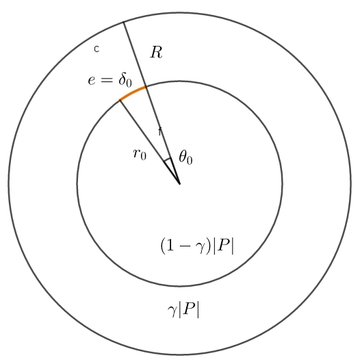
Figure 5: A rotation $\theta_{0}$ produces a mismatch $\delta_{0}$ to $\gamma|P|$ point pairs starting from $r_{0}$, when a uniform distributed PC is rotated around its center.

A justification for this simple derivation of the limit $\theta_{0}$ is that a rotation with $\theta_{0}<\theta$ of two identical uniformly distributed PCs produces a situation similar to a case of two i.i.d PCs at the outer zone $r_{0}<r$.

A simple ICP is assumed to succeed when:

$$\left(\frac{\delta}{\delta_{0}}\right)^{2}+\left(\frac{\theta}{\theta_{0}}\right)^{2}\leq 1,$$ (25)

where $\delta$ is the known magnitude $\delta=\|q\|$ of the known match $\tau([\omega],\theta,q)$ and $\theta$ is the known horizontal rotation from the correct match. This means that for a possible grid search or BnB approach, the two parameters $\lambda_{0}$ and $\theta_{0}$ define the grid granularity.

A complete misalignment has mean error $e$ between pairs of matching points $e\approx\delta_{0}$, and a complete alignment equals the registration noise $\epsilon$: $e\approx\epsilon$. The ICP match succeeds at the limit $\theta=\theta_{0}$ since the point density decreases, and the local $L_{0}$ increases, when scan radius $r$ grows, see the right detail of Fig. 1.

The BnB search grid can be set to a granularity, where the final attempt at the finest level of the search hierarchy can be safely done by a simple ICP. By this arrangement the BnB grid does not need to extend to actual tolerances sought after. Numerical values in our example data are $L_{0}=3.5$ m, $\gamma=0.6$, $\delta_{0}=1.75$ m and $R=35$ yielding $\theta_{0}=3.7^{o}$.

The convergence condition of Eq. 25 requires a verification. Fig. 6 summarizes a test setting, where matched PC pairs drawn from the data were artificially separated by $\tau(\theta,\delta q^{0})$, where translations were taken to several directions encoded by unit vectors $q^{0}$ to register the effect over the translation range $\delta$. Two contour lines with the match error $e=0.2$ m and $e=0.7$ m are shown. A successful match has $e\leq 0.2$ mm since this does contribute well to the desired final tree map accuracy. The point registration noise $\epsilon$ from the tree registration process is approximately $0.05<\epsilon<0.1$ m. The convergence area of the condition of Eq. 25 is inside the red arc. 200 PC pairs was used to produce the plot.

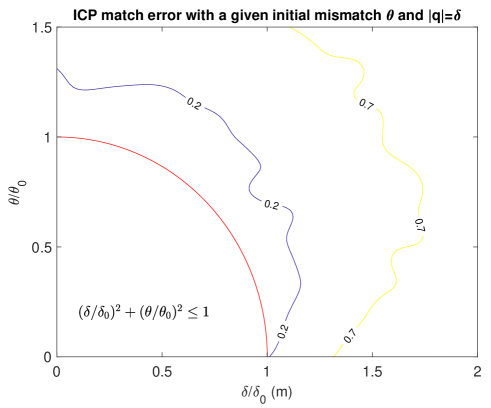
Figure 6: Match error $e$ (m) of a simple ICP method, when initial mismatch state $\tau(\theta,\delta)$ is known. The area inside the circle is where the convergence is quaranteed for uniform distributed PCs with $L_{0}=2\delta_{0}$.

The final values for the Go-ICP granularity coefficients are: $\sigma_{t}=\delta_{0}$ and $\sigma_{r}=\theta_{0}$. Each match uses an iteration stop criterion given in yang2015 and the only extra control layer is by monitoring that two PCs have enough geometric overlap in the matched configuration. The overlap $\lambda\approx 1-\gamma$, but a geometric calculation using view cone characteristics is used for the actual test. This is because PCs contain churn; trees obscure each other and some outliers occur everywhere in the scanning view. If $\lambda$ is not large enough, $\lambda<\lambda_{0}=0.4$, the frame pair $(i,j)$ will not be used in the iterative improvement of the matches.

The odometry is done in 3D and $\sigma_{r}$ concerns also the roll (and pitch) of the vehicle, even these had a negligible effect in point matching. This is because the point cloud is relatively flat, see Fig. 7. The Figure depicts also a limit chosen $\phi_{0}=8.2^{o}$ for a succesful match. This was found by a numerical test producing a similar plot as shown in Fig. 6. The size of $\phi_{0}$ indicates that the BnB search grid should be elongated (it is cubic grid in Go-ICP implementation). Very large rolls or pitch movements did not occur, and so we limited the BnB search space of rotation to $\pm 30^{o}$ horizontal zone and trusted that the hierarchical BnB quickly eliminates the useless search space. So, the final ICP convergence test is: $(\delta/\delta_{0})^{2}+(\theta/\theta_{0})^{2}+(\phi/\phi_{0})^{2}\leq 1$.

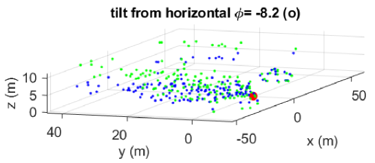
Figure 7: A demonstration of the found limit case for a rather certain ICP match to occur. The angle $\phi=8.2^{o}$ is the deviation from the vertical axis.

2.4 Iterative improvement

An initial tree registration and SLAM over sparse PCs is to be done at the autonomous vehicle. The aim of the initial SLAM is the immediate collision avoidance and basic orientation along the vehicle tasks goals. The PCs of selected views $V=\{(PC_{l},\tau_{l1}\}_{l=1...n}$ will be sent to the cloud environment, where an improvement of the map will occur.

The estimation of the overlap $\lambda$ is depicted in Fig. 8. Two vehicle poses $\tau_{i1}$ and $\tau_{j1}$ in views $V$ are depicted by their view cones. We noticed that the vertical dimension and the corresponding rotations corresponded very little to the final SLAM map via the match pair selection. Therefore e.g. the overlap analysis is done in a projective horizontal plane.

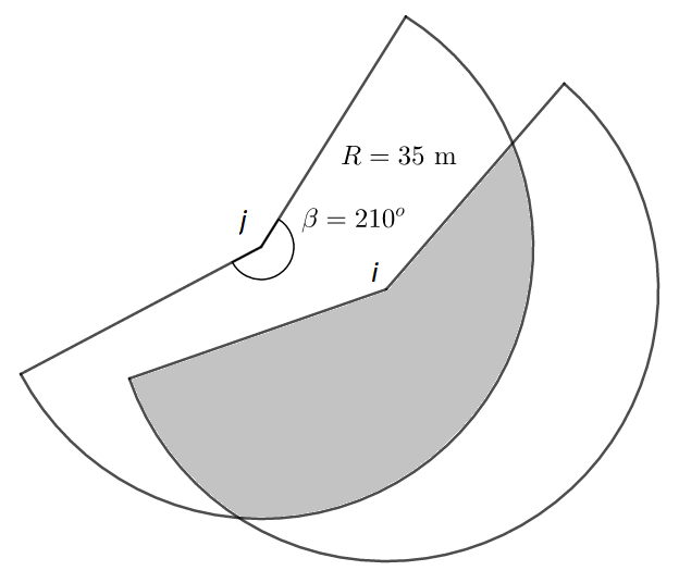
Figure 8: Overlap (gray area) can be estimated from the orientation and position only under an assumption of uniform PC distribution.

The process starts by selecting $m$ potential pairs of frames, which will be subjected to improvement. Fig. 9 depicts a scatter plot based on estimated overlap of views $V$ based on the relative view cone overlap $\lambda$ and the mean error $e(P_{j}t_{j1}\match P_{i}t_{i1})$ of the match, where non-overlapping parts are excluded. The maximum frame difference $\max i-j=1000$ and 0.2 % of the inspected 1870000 frames fall to a promising or acceptable set. The acceptable set was found by looking overlap ratios over $0.2<\lambda$ and checking the match error $e(P_{i}t_{i1}\match P_{j}t_{j1})$ of pairs $(i,j)$.

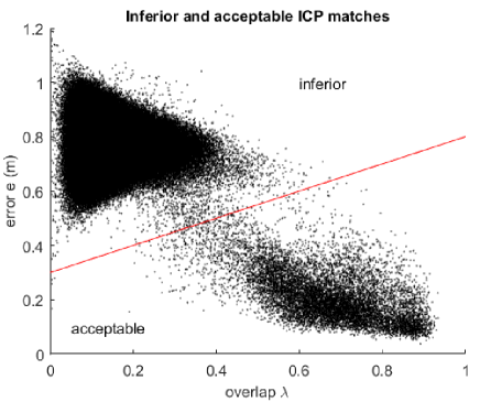
Figure 9: Scatter plot over ICP matches. An ICP match attempt either succeeds (acceptable) or is inferior (either fails completely or produces small overlap and large error.

The preliminary set $I_{2}\subset[1,n]\subset\mathbb{N}$ depicted by 3500 black dots is sampled to a subset of $m\approx 100$ nearly Poisson disk distributed pairs depicted by red circles in Fig. 10. The detail at the top of Fig. 10 is a schematic about how each black dot $\iota=(i,j)\in I_{2}$ relates to two frames $j$ and $i$. The nearly Poisson disc sampling was chosen since one can assume an individual sample will improve the surrounding pairs with equal amount everywhere. A mini-algorithm for producing a promising sample selection $I$ follows:

1. Test recent views $(P_{l},\tau_{l1})$ randomly and select pairs $(i,j)$ with $0.2<\lambda$. From those, select ones with the following condition fulfilled:

   $$e_{ij}<0.3\text{m}+\lambda_{ij}\times 0.5\text{m}$$ (26)

   and add $(i,j)\in I_{2}$. The inequality border is depicted by a red line in Fig. 9. Note that evaluation of values $e_{ij}$ and $\lambda_{ij}$ is relatively cheap, since the former comes from a direct nearest neighbor search and the latter is estimated directly from the parameters of transformations $\tau_{l1}(\theta_{l},{\vec{\omega}}_{l},p_{l})$ with $l\in\{i,j\}$.

2. Round $I_{2}$ to a set of grid points with spacing $\epsilon$. A set rounding operator $\{.\}_{\epsilon}$ is introduced for that purpose: $\{A\}_{\epsilon}=\{\text{round}(a/\epsilon)\epsilon\;|\,a\in A\}$ The spacing $\epsilon$ is decreased iteratively by $\epsilon:=0.8\epsilon$ until the size $|I_{1}|$ of the rounded set is closest to the intended size: $|I_{1}|\approx m$. The initial guess is $\epsilon=\sqrt{\text{boxareainFig.~{}\ref{fig:correctivePairs}}/m}$. With the final $\epsilon$:

   $$I_{1}=\{I_{2}\}_{\epsilon}$$ (27)

3. For each occupied grid point $\nu\in I_{1}$, choose the nearest match from the set $I_{2}$:

   $$I=\{\iota\,|\,\iota=\argmin_{\mu\in I_{2}}\|\mu-\nu\|,\,\nu\in I_{1}\}$$ (28)

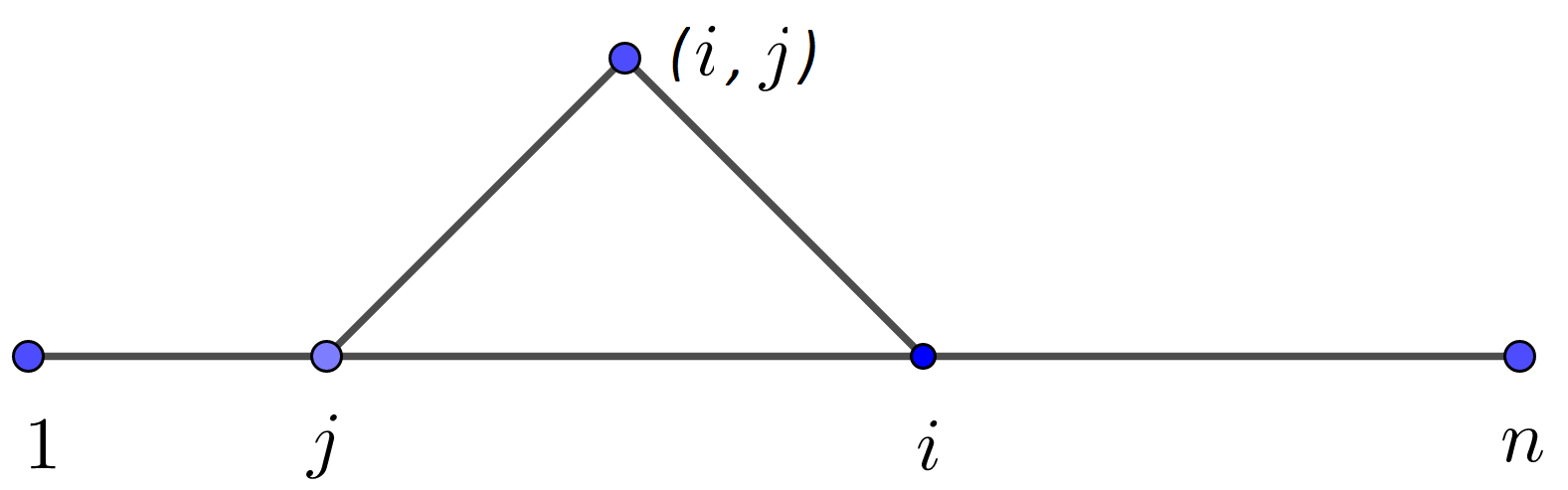
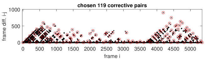
Figure 10: The selection of extra matches. Above: A match pairs $(i,j)$ representing a potential match is related to frames $i$ and $j$. The original SLAM proceeds along the abscissa from 1 to $n$ with $i=j+1$. Below: Set $I$ (red circles) of improvement matches with nearly Poisson disk distribution are chosen from 2800 potential match pairs of a set $I_{2}$ (black dots).

The main step of the algorithm applies Eq. 18 and Eq. 19 randomly until the whole set $I$ is exhausted or a convergence criterion is fulfilled. The simple SLAM is tried first. If it delivers a match error $e$ and an overlap $\lambda$ which do not fulfill the condition of Eq. 26, Go-ICP is called instead.

2.5 Quality criteria of the final map

Basically, there are two possible convergence criteria, one expressing the mean match error $e_{J}$ over a subset $J\subset I_{1}$, another one quantifying the quality of the final map. A measure useful for possible applications of tree maps is the tree registration noise $e_{C}$ nevalainen2020a . The registration noise is root mean square error (RMSE) of the tree cluster points from the arithmetic mean of the cluster.

This study focuses on finding the best possible transformations, so we use a numerically faster measure, which addresses the sharpness of the resulting map image. For that purpose, two grid factors $\epsilon_{1}=0.2$ m and $\epsilon_{2}=10.0$ m are chosen. The first one counts 1…4 grid points for a tree with a diameter $D=0.1...0.2$ m and the second one is conveniently larger than the mean distance between nearest trees $L_{0}=3.5$ m given in Section 2.3. One can define a blur ratio $0<\beta<1$:

$$\beta=\frac{|\{P\}_{\epsilon_{1}}|\epsilon_{1}^{2}}{|\{P\}_{\epsilon_{2}}|\epsilon_{2}^{2}},$$ (29)

where $P=\match_{l=1...n}P_{l}t_{l1}$ is the SLAM map, and $\{.\}_{\epsilon}$ is the set rounding operator originally defined for Eq. 27. The numerator of the ratio in Eq. 29 approximates the occupied area in the final map $P$ and the denominator estimates the overall area of the map.

The blur ratio $\beta$ is used as a target parameter to be minimized in the iterative improvement. It is related to the tree registration noise $e_{C}$ by having the minimae at the same time, but the absolute value of $\beta$ depends on how much undergrowth and small trees are on the site. Using $\beta$ in governing the improvement process is a novel feature, e.g. nevalainen2020a uses the registration noise $e_{C}$ instead, which requires alpha shape akkiraju1995 clustering. An tree clusters are detected by using $r_{\alpha}=0.5$ m as the alpha shape radius, and ignoring clusters with less than 15 points.

3 Results

The initial (top) and end state (bottom) of the final map $P=\cup_{l=1}^{n}{P_{l}t_{l1}}$ are depicted in Figure 11. Unlike with the ordinary ICP match $.\match.$, the associations between matching points have not been created but the map $P$ is just an unstructured PC. The odometric path is plotted in red.

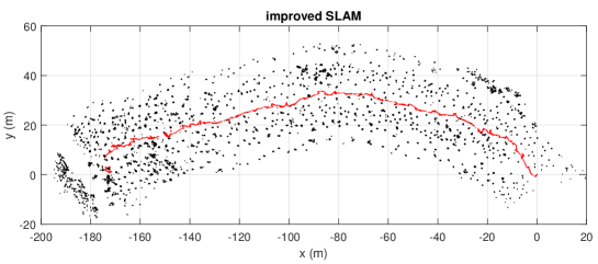
Figure 11: Above: the initial SLAM map. Below: the final map by the medium-gaps-first strategy.

The blur ratio $\beta$ of Eq. 29 moves from the initial $\beta=0.31$ of the top map of Figure 11 to $\beta=0.022$ of the end map at the bottom. A tree map of practical applications usually consists of tree cluster centers only, but for the sake of illustration, the registration points from all frames have been included. The initial scan on the top detail reaches up to 60 m distance while consistent tree registrations in the below map are within a 40 m stripe. The simplistic SLAM method pcregistericp() has a large rotation error, which is seen from the elongated tree clusters in the top details. The final map is the result of the medium-gaps-first strategy. Some blurred details are undergrowth and thickets.

The average stepwise match error $e=\mean_{k=2}^{n}e(P_{k-1}\match P_{k}t_{k\,k-1})$ was rather stable over the iterative improvement. This is probably because as some tree clusters get sharper during the process, some spread out due to registration errors. The order of choosing the corrective pairs of frames $\iota=(i,j)$ had a great effect. The strategy of choosing the smallest corrective steps first ($i-j$ in ascending order), ends to a worse end result $\beta=0.035$ than medium-gaps-first strategy, which reaches $\beta=0.022$. This result is depicted in Figure 11. Three strategies, medium-gaps-first, smallest-gaps-first and random choice are summarized in Table 1. The map noise $e_{C}$ is the RMSE of the tree cluster radius.

The map noise value found $e_{C}=0.15$ m is competitive when compared to a similar study tang2015 with $e_{C}\approx 0.2$ m and with more dense original scanning. The study areas also compare well, our area was $180\times 40\,\text{m}^{2}$ with approximately 600 trees and is gained from over a single open path.

Table 1: Evaluation times of two ICP methods.

Method	Blur factor (1)	RMSE error (m)	#Corrections (m)
Small-gaps-first	0.035	0.27	119
Medium-gaps-first	0.022	0.15	71
Random order	0.051	0.19	119

A Python implementation of Go-ICP pygoicp was used. The average run time was 0.41 secs over 29 Go-ICP runs triggered. The average size of the PCs was 131 points making the Go-ICP quite fast.

Table 2: Evaluation times of two ICP methods.

Method	One call (sec)	Number of calls
Go-ICP	0.41	29
pcregistericp	0.19	80

The standard Go-ICP yang2015 uses much smaller coefficients $\sigma_{r}$ and $\sigma_{t}$, since it is not specialized to near uniform PCs. Also, we found that the tilt $\phi$ from the vertical axis of the vehicle is limited to $\phi\in[-\pi/6,\pi/6]$ and this further reduces the BnB search space. These advantages are summarized in Table 3. The translation granularity $\sigma_{t}$ is computed in yang2015 by $\sigma_{t}=10^{-4}\times N\times L/2$ where $N\approx 130$ is the data point number and $L\approx 180$ m is the largest included diameter of the PC. This gives an automated value $\sigma_{t}=1.2$ m. The translation search was limited to $10\times 10\times 2\text{m}^{3}$ volume in both cases.

Table 3: The BnB search space reduction, when Go-ICP gets adapted to the nearly sparse uniform PCs.

PC type	Horiz. zone (o)	Rot. granul. $\sigma_{r}$ (o)	Transl. granul. $\sigma_{t}$ (m)	BnB size
General	180	1.0	1.2	$350\times 10^{6}$
Sparse uniform	60	3.7	1.9	$1.5\times 10^{6}$

4 Discussion

More experiments are needed in deciding a sensible strategy over the application order of improvement matches. The medium-gaps-first strategy is just a best found for this particular task, and obviously there is need for some sort of control, e.g. an end condition to stop the divergence when the blur ratio $\beta$ does not improve anymore. A probabilistic way for optimizing both the selection and ordering of the set $I$ of the frame pairs could arise by applying e.g. probabilistic data association bowman2017 to Delaunay triangle stars used in li2020a .

The data nevalainen2020b used is a recording of a forest harvester operation nevalainen2020a . Although the data allowed in developing some parts of the pipeline, crucial parts are missing. These are: the aforementioned search for the fastest converging sequence of corrections, functional memory management of recent scanner views and a process converting individual views to a memoized global map li2020a , and countering possible systematical errors in relatively simplistic tree registration method presented in nevalainen2020a , which was used to generate the test data nevalainen2020b .

Since the pcregistericp() calls dominate (2800 initial matches edge-computed and 80 corrective matches versus 29 Go-ICP calls), the combined time stays tolerable and promising for a possible full implementation. The 2800 initial matches is to be edge-computed at the vehicle, and therefore this process is likely a subject of many optimizations concerning the sensors, application specific integrated circuits (ASIC) and algorithmic developments liu2019 .

The blur ratio $\beta$ of Eq. 29 is very close to the dimensionality estimation by box counting wu2020 . The iteration starts with a box counting dimension estimate $d=1.4$ and gets stagnated to $d\approx 1$ for a long time while cluster archs of individual trees get shorter, see the top detail of Fig. 11. Then dimensionality moves to the final $d=0.3$. PC dimensionality would be a better iteration progress indicator in that it does not require specific parameters $\epsilon_{1}$ and $\epsilon_{2}$. Both indicators $\beta$ and $d$ apply in the 2D (projective maps) and 3D cases by a change of the power of $\epsilon$ in Eq. 29.

The search space reduction (230:1) showin in Table 3 has large but indirect effect to the computation, since the BnB process is hierarchical and eliminates large swath of search space rather soon. The reduction in computation time seems to be in the range of 3:1 … 10:1, when uniformity assumptions are applied.

From the point of view of lightweight computation at the edge and cloud offloading in remote environments, the method we have proposed in this paper presents some inherent benefits. First, by providing a self-corrective approach there is potential to minimizing the drift in localization for autonomous mobile robots operating over large distances in places with a weak or missing Global Navigation Satellite System performance (GNSS-denied environments). For example, UAVs flying under tree canopy in forests for surveying applications that cannot rely on GNSS sensors are a potential application area. Second, by minimizing the size of the PC used for correcting the odometry process, we can provide cloud offloading or multi-robot collaboration even in environments where connectivity is poor and unreliable and latency does not allow for traditional computational offloading. Therefore, large-scale maps can be built at the cloud or within multi-robot systems in remote environments.

Finally, it is worth mentioning that this method can be extended to multiple domains and application areas. From the perspective of the low computational complexity, this method can extend long-term autonomy in mobile robots by reducing the embedded hardware requirements. This in turn related to lower energy consumption and applicability in smaller platforms. Moreover, if landmarks or anchors are well identified, this can also be leveraged within collaborative multi-robot systems, e.g., with micro-aerial vehicles being deployed from ground units in remote environments queralta2020sarmrs . In forests environments in particular, our adaptive and lightweight self-corrective SLAM approach can be used for either canopy or tree stem registration, but other features that are distributed throughout the operational environments could be exploited as well.

The next two Subsections are devoted to the discussion of alternative details of the Methods section.

4.1 Alternatives for power coefficients

The choice of power coefficient $u_{l}$ seems to have great effect on the proposed iterative improvement scheme. Just as there are alternatives to the proposed interpolation scheme zefrani1998 , there are alternatives for the formulation of $u_{l}$ defined in Eq. 20:

1. Cumulative measures like the relative odometric path length $u_{l}=\sum_{k=j+1}^{l}\|q_{k}-q_{k-1}\|/\sum_{k=j+1}^{n}\|q_{k}-q_{k-1}\|$ of transformations $\tau_{k1}([omega_{k}],\theta_{k},q_{k})$ or accumulated match errors: $u_{l}=\sum_{k=j+1}^{l}e_{k}/\sum_{k=j+1}^{n}e_{k}$.

2. A more sophisticated SE(3) metrics. One candidate is a linear combination of relative rotation and translation park1995 $d(\tau_{lj})=\sqrt{a\theta_{lj}^{2}+b\|q_{lj}\|^{2}}$, where $\tau_{lj}=\tau_{lj}(\theta_{lj},\vec{\omega}_{lj},q_{lj})$ and $0<a,b\in\mathbb{R}$ are free positive constants. This leads to:

   $$u_{l}=\frac{d(\tau_{lj})}{d(\tau_{ij})}.$$ (30)

   If the scanner view cone is known, the above measure is very close to the mean squared distance between corresponding spots in the two view cones.

3. For paths with a lot of loops, one can find the nearest fit from the skew path $\{\tau_{u}\,|\tau_{j1}^{1-u}\tau_{i1}^{u}\}_{0\leq u\leq 1}$ shown in Figure 2:

   $$u_{l}=\argmin_{u}d(\tau_{u}^{-1}\tau_{lj}),$$ (31)

   where $\tau_{u}^{-1}\tau_{lj}$ is a transformation from $\tau_{lj}$ to $\tau_{u}$.

4.2 Frame elimination

After the iterative improvement, some frames may show a large detrimental contribution to the final map quality. These frames can be removed. For this, one has to reshuffle the summation of the map error $e_{C}$ to individual frames $l,\,1\leq l\leq n$:

$$e_{C}^{2}=\mean_{i\in[1,n],p\in{P_{i}}^{\prime}}\|p-c_{h_{i}}\|^{2}=\sum_{i=1}^{n}w_{i},$$ (32)

where an inclusion of $p\in P_{i}^{\prime}\subset P_{i}$ occurs only if it contributes to some tree in the final map and $w_{i}$ are the rearranged summand parts of the mean. The largest values can be removed. Finding a subset of frames to be removed is a combinatorially expensive operation, which should be done only if the application specifically requires it. Removing low-quality frames has similarities with the problem of selecting and ordering the corrective frame pairs; and both problems resemble feature selection over large feature space in general Machine Learning.

5 Conclusion

This article gives a complete presentation of mathematical details of rigid body interpolation and its application to iterative SLAM improvement. A main motivation was to provide a unified approach to the SLAM accuracy improvement. This resulted in an outline of the proposed iterative improvement algorithm. The second motivation was to test how much the very reliable Go-ICP algorithm can gain advantage from the small and sparse problems. It seems that Go-ICP is a feasible choice for tree map related SLAM.

Our results suggest that the iterative SLAM improvement using rigid body interpolation proposed in this paper has potential for many applications with sparse PCs, whether point clouds are key points, sets of beacons or subsampled PCs. The near uniform distribution makes the BnB search grid of Go-ICP coarser, and this and small PC size speeds up Go-ICP, which is otherwise known to be a rather slow method. The sensor fusion with GNSS, inertial mass units and other sensors has been left out to keep the presentation simple.

More research is needed especially about an optimal selection of the improvement matches before an effort to build a true pipeline from autonomous vehicle to a cloud environment can be done. The pipeline would cover the edge-computed tree registration and SLAM, transmission of sparse PCs to the cloud computing environment and the iterative tree map improvement. This may take years, but could be worth of an effort.

- [1] Tixiao Shan and Brendan Englot. Lego-loam: Lightweight and ground-optimized lidar odometry and mapping on variable terrain. In 2018 IEEE/RSJ International Conference on Intelligent Robots and Systems (IROS), pages 4758–4765. IEEE, 2018.
- [2] Tong Qin, Peiliang Li, and Shaojie Shen. Vins-mono: A robust and versatile monocular visual-inertial state estimator. IEEE Transactions on Robotics, 34(4):1004–1020, 2018.
- [3] Jorge Peña Queralta, Li Qingqing, Fabrizio Schiano, and Tomi Westerlund. Vio-uwb-based collaborative localization and dense scene reconstruction within heterogeneous multi-robot systems. 2020.
- [4] Qingqing Li, Paavo Nevalainen, Jorge Peña Queralta, Jukka Heikkonen, and Tomi Westerlund. Localization in Unstructured Environments: Towards Autonomous Robots in Forests with Delaunay Triangulation. arXiv e-prints, page arXiv:2005.05662, May 2020.
- [5] J. Engel, V. Koltun, and D. Cremers. Direct sparse odometry. IEEE Transactions on Pattern Analysis and Machine Intelligence, 40(3):611–625, 2018.
- [6] D. Chetverikov, D. Svirko, Dmitry Stepanov, and Pavel Krsek. The trimmed iterative closest point algorithm. volume 16, pages 545– 548 vol.3, 02 2002.
- [7] Jiaolong Yang, Hongdong li, Dylan Campbell, and Yunde Jia. Go-icp: A globally optimal solution to 3d icp point-set registration. IEEE Transactions on Pattern Analysis and Machine Intelligence, 38:1–1, 12 2015.
- [8] The Mathworks, Inc., Natick, Massachusetts. MATLAB version 9.8.0.1323502 (R2020a), 2020.
- [9] Brian Williams, Mark Cummins, José Neira, Paul Newman, Ian Reid, and Juan Tardos. A comparison of loop closing techniques in monocular slam. Robotics and Autonomous Systems, 57:1188–1197, 12 2009.
- [10] Z. Wang, Y. Shen, B. Cai, and M. T. Saleem. A brief review on loop closure detection with 3d point cloud. In 2019 IEEE International Conference on Real-time Computing and Robotics (RCAR), pages 929–934, 2019.
- [11] Ryan A Chisholm, Jinqiang Cui, Shawn KY Lum, and Ben M Chen. Uav lidar for below-canopy forest surveys. Journal of Unmanned Vehicle Systems, 1(01):61–68, 2013.
- [12] Temuulen Sankey, Jonathon Donager, Jason McVay, and Joel B Sankey. Uav lidar and hyperspectral fusion for forest monitoring in the southwestern usa. Remote Sensing of Environment, 195:30–43, 2017.
- [13] A Ortiz Arteaga, D Scott, and J Boehm. Initial investigation of a low-cost automotive lidar system. In ISPRS-International Archives of the Photogrammetry, Remote Sensing and Spatial Information Sciences, volume 42, pages 233–240. Copernicus GmbH, 2019.
- [14] Jiarong Lin and Fu Zhang. Loam livox: A fast, robust, high-precision lidar odometry and mapping package for lidars of small fov. In 2020 IEEE International Conference on Robotics and Automation (ICRA), pages 3126–3131. IEEE, 2020.
- [15] Erik Einhorn and Horst-Michael Gross. Generic ndt mapping in dynamic environments and its application for lifelong slam. Robotics and Autonomous Systems, 69:28–39, 2015.
- [16] Kevin M Lynch and Frank C. Park. Modern Robotics: Mechanics, Planning, and Control. Cambridge Univeristy Press, 2017.
- [17] Yang Chen and Gérard Medioni. Object modelling by registration of multiple range images. Image Vision Comput., 10(3):145–155, Apr 1992.
- [18] P. J. Besl and N. D. McKay. A method for registration of 3-d shapes. IEEE Transactions on Pattern Analysis and Machine Intelligence, 14(2):239–256, 1992.
- [19] Cleve Moler and Charles Loan. Nineteen dubious ways to compute the exponential of a matrix, twenty-five years later. Society for Industrial and Applied Mathematics, 45:3–49, 03 2003.
- [20] Leo Dorst, Daniel Fontijne, and Stephen Mann. Geometric Algebra for Computer Science: An Object-Oriented Approach to Geometry. Morgan Kaufmann Publishers Inc., San Francisco, CA, USA, 2009.
- [21] Neil T. Dantam. Practical exponential coordinates using implicit dual quaternions. In Workshop on the Algorithmic Foundations of Robotics, pages 639–655, 2018.
- [22] Paavo Nevalainen, Qingqing LI, Timo Melkas, Kirsi Riekki, Tomi Westerlund, and Jukka Heikkonen. Navigation and mapping in forest environment using sparse point clouds. Remote Sensing, 12(24), 2020.
- [23] N. Akkiraju, H. Edelsbrunner, M. Facelo, E. P. Mücke P. Fu, and C. Varela. Alpha shapes: definition and software. In N. Amenta, editor, Proc. Internat. Comput. Geom. Software Workshop. Geometry Center Res. Rept., 1995.
- [24] Jian Tang, Yuwei Chen, Antero Kukko, Harri Kaartinen, Anttoni Jaakkola, Ehsan Khoramshahi, Teemu Hakala, Juha Hyyppä, Markus Holopainen, and Hannu Hyyppä. SLAM aided stem mapping for forest inventory with small-footprint mobile LiDAR. Forests, 6(12):4588–4606, 12 2015.
- [25] py-goicp implementation, howpublished = https://pypi.org/project/py-goicp/, note = Accessed: 2020-12-30.
- [26] S. L. Bowman, N. Atanasov, K. Daniilidis, and G. J. Pappas. Probabilistic data association for semantic slam. In 2017 IEEE International Conference on Robotics and Automation (ICRA), pages 1722–1729, 2017.
- [27] Paavo Nevalainen. Replication data for: Navigation and mapping in forest environment using sparse point clouds. http://dx.doi.org/10.4225/13/511C71F8612C3, 2020.
- [28] Runze Liu, Jianlei Yang, Yiran Chen, and Weisheng Zhao. eSLAM: An Energy-Efficient Accelerator for Real-Time ORB-SLAM on FPGA Platform. arXiv e-prints, page arXiv:1906.05096, June 2019.
- [29] Jiaxin Wu, Xin Jin, Shuo Mi, and Jinbo Tang. An effective method to compute the box-counting dimension based on the mathematical definition and intervals. Results in Engineering, 6:100106, 2020.
- [30] Jorge Peña Queralta, Jussi Taipalmaa, Bilge Can Pullinen, Victor Kathan Sarker, Tuan Nguyen Gia, Hannu Tenhunen, Moncef Gabbouj, Jenni Raitoharju, and Tomi Westerlund. Collaborative multi-robot search and rescue: Planning, coordination, perception and active vision. IEEE Access, 8:191617–191643, 2020.
- [31] Miloš Žefran and Vijay Kumar. Interpolation schemes for rigid body motions. Computer-Aided Design, 30(3):179 – 189, 1998. Motion Design and Kinematics.
- [32] F. C. Park. Distance Metrics on the Rigid-Body Motions with Applications to Mechanism Design. Journal of Mechanical Design, 117(1):48–54, 03 1995.