Metastable Helium Absorptions with 3D Hydrodynamics and
Self-Consistent Photochemistry I:
WASP-69b, Dimensionality, XUV Flux Level, Spectral Types, and Flares

Abstract

The metastable Helium ($\mathrm{He}^{*}$) lines near $10830~{}\text{\AA}$ are ideal probes of atmospheric erosion–a common phenomenon of close-in exoplanet evolution. A handful of exoplanet observations yielded well-resolved $\mathrm{He}^{*}$ absorption features in transits, yet they were mostly analyzed with 1D isothermal models prescribing mass-loss rates. This work devises 3D hydrodynamics co-evolved with ray-tracing radiative transfer and non-equilibrium thermochemsitry. Starting from the observed stellar/planetary properties with reasonable assumptions about the host’s high energy irradiation, we predict from first principle the mass loss rate, the temperature and ionization profiles, and 3D outflow kinematics. Our simulations well reproduce the observed $\mathrm{He}^{*}$ line profiles and light curves of WASP-69b. We further investigate the dependence of $\mathrm{He}^{*}$ observables on simulation conditions and host radiation. The key findings are: (1) Simulations reveal a photoevaporative outflow ($\sim 0.5~{}M_{\oplus}~{}{\rm Gyr}^{-1}$) for WASP-69b without a prominent comet-like tail, consistent with the symmetric transit shape (Vissapragada et al., 2020). (2) 3D simulations are mandatory for hydrodynamic features, including Coriolis force, advection, and kinematic line broadening. (3) EUV ($>13.6~{}\mathrm{eV}$) photons dominate photoevaporative outflows and populate $\mathrm{He}^{*}$ via recombination; FUV is also detrimental by destroying $\mathrm{He}^{*}$; X-ray plays a secondary role. (4) K stars hit the sweet spot of EUV/FUV balance for $\mathrm{He}^{*}$ line observation, while G and M stars are also worthy targets. (5) Stellar flars create characteristic responses in the $\mathrm{He}^{*}$ line profiles.

1 Introduction

One of the most exciting discoveries in exoplanetary sciences in recent years is that the radii of sub-Neptune planets have a bimodal distribution (Fulton et al., 2017). The prevailing explanation is the atmospheric erosion by either photoevaporation (e.g. Owen & Wu, 2013, 2017) or core-powered mass loss (Ginzburg et al., 2018; Gupta & Schlichting, 2019, 2020). In any case, the prominence of the radius gap implies that atmospheric erosion is probably a stage of evolution that close-in exoplanets very commonly go through. Since the discovery of the Lyman $\alpha$ (Ly$\alpha~{}$hereafter) transit of hot Jupiter HD209458 b (Vidal-Madjar et al., 2003), Ly$\alpha~{}$has been a workhorse for studying atmospheric erosion (e.g. Lecavelier Des Etangs et al., 2010; Kulow et al., 2014). However, Ly$\alpha~{}$has some unavoidable limitations, namely, it is heavily contaminated by geocoronal emission, and interstellar absorption saturating the very center of the line (e.g. Ehrenreich et al., 2015). Moreover, one has to go space to observe this UV transition. These effects significantly limit the number of systems for which we can study Ly$\alpha~{}$transits.

Besides Ly$\alpha~{}$, helium lines are emerging as promising outflow indicators. The $2^{3}$S state of helium is often called the “metastable state” ($\mathrm{He}^{*}$ hereafter), because the $2^{3}$S$\rightarrow 1^{1}$S transition is a magnetic dipole process with a slow spontaneous decay rate of $A\simeq 1.3\times 10^{-3}~{}\mathrm{s}^{-1}$ (Drake, 1971, 2006). Meanwhile, the transition between the lower $2^{3}$S and the upper $2^{3}$P_J states of helium consists of three lines with $A>10^{7}~{}\mathrm{s}^{-1}$, whose wavelengths in vacuum are $10832.08~{}\text{\AA}$ (for the $J=0$ upper state), $10833.24~{}\text{\AA}$ ($J=1$), and $10833.33~{}\text{\AA}$ ($J=2$) respectively. These lines are often referred to as “He i $10830~{}\text{\AA}$ lines” or the “metastable helium lines”, as they are radiatively decoupled from the ground state. The abundance of helium, the absence of geocoronal or intersteallar containmination, the longevity of metastable state, and observability from the ground together enabled the $\mathrm{He}^{*}$ lines as an excellent probe of ionized flows in various scenarios of astrophysics, including quasars (e.g. Leighly et al., 2011), stellar atmospheres and outflows (see Edwards et al., 2003, and references to the article), and T Tauri stars (Kwan et al., 2007).

Over the years, researchers have proposed the $\mathrm{He}^{*}$ lines as a tracer of mass loss of close-in exoplanets (Seager & Sasselov, 2000; Turner et al., 2016; Oklopčić & Hirata, 2018). It was the secure detection of Spake et al. (2018) that revitalized interest in this unique transition. At the time of writing this paper, several close-in exoplanets have transmission $\mathrm{He}^{*}$ line profiles resolved by ground-based spectrographs (e.g. Allart et al., 2018; Nortmann et al., 2018; Salz et al., 2018; Kirk et al., 2020; Ninan et al., 2020). More recently, Vissapragada et al. (2020) custom made a narrow band filter specifically for the $\mathrm{He}^{*}$ transitions on the diffuser-based photometric system on Palomar/WIRC. The resultant precise light curves of the $\mathrm{He}^{*}$ is complementary to the line profiles from the near-infradred spectrographs. A lot of information about atmospheric outflow is hiding in these line profiles and light curves waiting to be interpreted. The models that are commonly used in the literature to interpret these $\mathrm{He}^{*}$ observations are 1D spherical symmetric models that are isothermal (Oklopčić & Hirata, 2018; Oklopčić, 2019; Palle et al., 2020), or have prescribed heating efficiency (Lampón et al., 2020). The model is widely recognized for its simplicity and effectiveness, however it has to prescribe, rather than predict, a mass loss rate or a temperature profile.

In this work, we build upon our previous model that conducts hydrodynamics, self-consistent thermochemistry, and ray-tracing radiative transfer to study the photoevaporation of sub-Neptune planets (Wang & Dai, 2018, WD18 hereafter). We have streamlined the code so that it is sufficiently fast to run in 3D to fully capture outflow dynamics, and added various processes that are relevant to the (de)population of $\mathrm{He}^{*}$. We will show in this paper that using the observed stellar/planetary properties and making reasonable estimate of the high energy spectral energy distribution (SED) about the host star, our model can predict mass loss rate, the temperature profile, the ionization states, and synthesize the observed $\mathrm{He}^{*}$ line observables from first principles.

In this first work of a series, we focus on WASP-69b, which is one of the first detections of $\mathrm{He}^{*}$ line absorption with well-resolved line profile (Nortmann et al., 2018). Acknowledging the many limitations of a 1D isothermal model, Nortmann et al. (2018) did not tie their $\mathrm{He}^{*}$ line observation with a theoretical model. Instead they only reported what the data showed directly. Notably, Nortmann et al. (2018) reported an asymmetric transit profile characterized by a longer-than-expected egress that could be caused by a comet-like tail associated with the mass loss. However, Vissapragada et al. (2020) suggests a symmetric shape of transit using better-sampled light curves with higher precision and signal-to-noise ratio (SNR). Another interesting point about WASP-69b is the apparent temporal variability of the $\mathrm{He}^{*}$ transit depth seen in Nortmann et al. (2018). We will try to understand these observations of WASP-69b in the framework of our 3D hydrodynamic simulations. Afterwards, we will use WASP-69 as a fiducial case to investigate the impact of dimensionality, XUV flux level, and host spectral types on the observables of the $\mathrm{He}^{*}$ lines.

This paper is structured as follows. §2 describes our methods of numerical simulations and synthetic observations. In §3, we present a fiducial model of WASP-69b that well reproduces all current observations. Based on this model, §4 studies how various system parameters impact the rate of photoevaporation and $\mathrm{He}^{*}$ observables. §5 explores the possibility that stellar flare may cause the observed temporal variability of WASP-69b. §6 summarizes the findings of this paper.

2 Methods

2.1 Basic Setup

We conceptually divided a planet into four regions: (1) a dense core, (2) a convective inner atmosphere, (3) a quasi-isothermal outer atmosphere with equilibrium temperature $T_{\mathrm{eq}}$ and (4) an outflowing region irradiated by high energy photons (e.g. Rafikov, 2006; Ginzburg et al., 2016; Owen & Wu, 2016). The equilibrium temperature $T_{\mathrm{eq}}$ satisfies,

$$T_{\mathrm{eq}}\simeq 886~{}\mathrm{K}\left(\dfrac{L_{*}}{L_{\odot}}\right)^{1/4}\left(\dfrac{a}{0.1~{}\mathrm{AU}}\right)^{-1/2}\ ,$$ (1)

where $L_{*}$ is the bolometric luminosity of the star, and $a$ is the semi-major axis of the planetary orbit. Our simulations will focus on regions (3) and (4), whereas the structure of regions (1) and (2) provide the correct boundary conditions crucial for correctly reproducing the measured mass and radius of the planet. We refer the reader to Appendix A for the details of how we set up the internal structures of our planet and resultant boundary conditions for our simulations.

We characterize the high energy radiation spectral energy distribution (SED) of the host star with 5 different characteristic energy bins: (1) $h\nu=2~{}\mathrm{eV}$ for infrared, optical and near ultraviolet (NUV) photons, (2) $h\nu=7~{}\mathrm{eV}$ for “soft” far ultraviolet (FUV) photons that can photoionize $\mathrm{He}^{*}$, (3) $h\nu=12~{}\mathrm{eV}$ for the Lyman-Werner band FUV photons that can photodissociate molecular hydrogen, (4) $h\nu=20~{}\mathrm{eV}$ for “soft” extreme ultraviolet (soft EUV) photons that can ionize hydrogen but not helium, (5) $h\nu=40~{}\mathrm{eV}$ for hard EUV photons that ionize hydrogen and helium, and (6) $h\nu=3~{}\mathrm{keV}$ for the X-ray.

Our simulation combines ray-tracing radiative transfer, real-time non-equilibrium thermochemistry, and full hydrodynamics calculations (based on a higher order Godunov hydrodynamic solver Athena++; Stone et al. 2020). The simulation is mostly based on our WD18 work with a few modifications and improvements added for the higher dimensionality and the inclusion of $\mathrm{He}^{*}$.

2.2 Geometry and Boundary Conditions

The density distribution, temperature profile and the dynamics of outflowing atmosphere all play a part in the $\mathrm{He}^{*}$ observables. To capture the outflow dynamics accurately, simulations should include the gravity of the star and the planet and the effects of orbital motion: the centrifugal and Coriolis forces. Therefore, 3D simulations are required. Given its short orbital period and observed radial velocities (Anderson et al., 2014), we assume that WASP-69b is tidally locked and circularized. Our simulation is run in a co-rotating frame centered on the planet. We adopt a spherical polar coordinate $(r,\theta,\phi)$ with $\theta=0$ pointing towards the host star and $\phi=0$ pointing in the direction of orbital motion.

The mesh covers the domain $(r,\theta,\phi)\in[r_{\rm in},r_{\rm out}]\otimes[0,\pi]\otimes[0,\pi]$. Planet-specific radial boundaries $r_{\rm in}$ and $r_{\rm out}$ usually extend from the the base of the quasi-isothermal layer to a relatively large radii (150 $R_{\oplus}$ in this case) such that the density/opacity drops low enough. The radial grids are placed logarithmically to strategically capture the steep change of density, while latitudinal and azimuthal grids are spaced evenly. Reflecting boundary conditions are enforced at the $r=r_{\rm in}$, $\phi=0$ and $\phi=\pi$ boundaries, while the $r=r_{\rm out}$ boundary is an outflowing boundary. The $\theta=0$, $\theta=\pi$ boundaries are polar wedges to avoid coordinate singularity. The whole mesh, with its polar axis always pointing towards the host star, co-rotates with the orbital motion and the rotation of the tidally-locked planet.

In a 3D spherical polar mesh, the grids near the polar axis are narrow in the azimuthal direction ($\delta x_{\phi}\simeq r_{\rm cc}\sin\theta_{\rm cc}\delta\phi$; subscripts “cc” stand for “cell center”). This can result in highly non-unitary aspect ratios ($\delta x_{\theta}\simeq r_{\rm cc}\delta\theta$), and a stringent Courant-Friedrichs-Lewy (CFL) condition. We thus introduce an adaptive “mesh coarsening” technique for the azimuthal grids near the poles. Without any violations of conservation laws, the effective aspect ratio of the high-latitude zones become close to one and the timestep constraints imposed by CFL condition is not as severe (see also Nakamura et al., 2019; Müller et al., 2019). This helps to greatly speed up our model.

2.3 $\mathrm{He}^{*}$ in non-LTE Thermochemistry

Our simulation includes a non-local-thermodynamic-equilibrium reaction network that coevolves with the hydrodynamics (see WD18 for detail). With the addition of the metastable state of neutral helium and all relevant reactions that populate and de-populate this state (see Oklopčić & Hirata 2018 and references therein). Our reaction network now has 26 thermochemical “species” (24 chemical species in WD18, $\mathrm{He}^{*}$, and internal energy density) and 135 reactions such as ionization, recombination, collisional (de-)excitation, photodissociation, and cooling and heating processes. The ordinary differential equations (ODEs) of the thermochemical network were solved efficiently using the semi-implicit method specially optimized for the graphics processing units (GPUs). The resultant efficiency allows us to coevolve the hydrodynamics with the thermodynamics, rather than including thermodynamics as a post-processing step that is often done in the literature. Again, we refer interested readers to WD18 for more details.

2.4 Synthetic Observations

We synthesize both the transmission line profiles (Nortmann et al., 2018) and the narrow-band light curves (Vissapragada et al., 2020) of $\mathrm{He}^{*}$ transitions using our simulations. At each wavelength $\lambda$ and a particular orbital phase, the optical depth along a line of sight (LoS hereafter) is given by,

$$\begin{split}\tau(\lambda;\Phi)=\int&|\mathrm{d}\mathbf{x}|\ n(\mathrm{He}^{*};\mathbf{x};\Phi)\\ &\times\sum_{i}\sigma_{i}[\lambda;\hat{n}_{\rm LoS}\cdot\mathbf{v}(\mathbf{x};\Phi),T(\mathbf{x};\Phi)]\ .\end{split}$$ (2)

where we have transformed from our planet-centered coordinate systems in the simulations to a star-centered coordinate system for the synthetic observations. Thus $\mathbf{x}$ and $\mathbf{v}$ are the position and velocity vector measured from the host star. The integration goes along the designated LoS, and the summation index $i$ runs over $\mathrm{He}^{*}$’s three lines with different upper state quantum number $J$. The cross-section $\sigma_{i}$ is assumed to be a Voigt profile which convolves the intrinsic Lorentz profile ($\gamma=A/4\pi$, $A=1.0216\times 10^{7}\ \mathrm{s}^{-1}$; see Drake 2006) with a Gaussian profile from thermal broadening at temperature $T(\mathbf{x})$. This Voigt profile is shifted by the local bulk velocity including orbital motion and outflow kinematics and the projection onto the LoS $\hat{n}_{\rm LoS}\cdot\mathbf{v}(\mathbf{x})$.

This integration is performed for all relevant LoS that originate from the surface of the host star:

$$\epsilon(\lambda;\Phi)=1-\int\mathrm{d}\Sigma\ S\mathrm{e}^{-\tau(\lambda;\Phi)}\ ,$$ (3)

where $\epsilon(\lambda)$ is the relative extinction at wavelength $\lambda$, $S(\lambda)$ is the normalized surface brightness ($\int\mathrm{d}\Sigma S(\lambda)=1$) of the star after accounting for limb darkening and stellar rotation. The integral runs through the entire projected stellar surface.

$\epsilon(\lambda;\Phi)$ is the absorption line profile as a function of wavelength and orbital phase (time). We mimic what observers often do in $\mathrm{He}^{*}$ observations i.e. time averaging $\epsilon(\lambda;\Phi)$ over the entire transit event from nominal ingress to egress ($t_{\textsc{{ii}}}$ through $t_{\textsc{{iii}}}$). The outcome $\Delta\epsilon(\lambda)$ is a line profile of excess absorption to be compared with observations directly.

We report a number of summary statistics including the equivalent widths $\langle W_{\lambda}\rangle\equiv\int\Delta\epsilon(\lambda)~{}\mathrm{d}\lambda$, the radial velocity shift of the absorption peak $\Delta v_{\rm peak}$ and the full-width-half-maximum (FWHM) of the absorption line profile. These summary statistics help us to compare between models and observations efficiently and are less prone to measurement uncertainty, bad pixels and other instrumental effects.

Finally, we integrated $\epsilon(\lambda;\Phi)$ multiplied by a filter bandpass function over $\lambda$. The result is a transit light curve near the $\mathrm{He}^{*}$ transitions. In this work, we use the bandpass function provided by Vissapragada et al. (2020) for a direct comparison with their results.

3 Fiducial Model of WASP-69b

Table 1: Properties of the fiducial model for WASP-69b

Item	Value
Simulation domain
Radial range	$11.37\leq(r/R_{\oplus})\leq\ 150$
Latitudinal range	$0\leq\theta\leq\pi$
Azimuthal range	$0\leq\phi\leq\pi$
Resolution $(N_{\log r}\times N_{\theta}\times N_{\phi})$	$144\times 128\times 64$
Planet interior†
$M_{\mathrm{rcb}}$	$82.6~{}M_{\oplus}$
$\langle r_{\mathrm{eff}}\rangle$	$11.8~{}R_{\oplus}$
Radiation flux [photon $\mathrm{cm}~{}^{-2}~{}\mathrm{s}^{-1}$]
$2~{}\mathrm{eV}$ (IR/optical)	$6.4\times 10^{19}$
$7~{}\mathrm{eV}$ (Soft FUV)	$6\times 10^{15}$
$12~{}\mathrm{eV}$ (LW)	$1\times 10^{12}$
$20~{}\mathrm{eV}$ (Soft EUV) ‡	$5\times 10^{12}$
$40~{}\mathrm{eV}$ (Hard EUV) ‡	$3\times 10^{13}$
$3~{}\mathrm{keV}$ (X-ray) ‡	$1.2\times 10^{12}$
Initial abundances [$n_{\mathrm{X}}/n_{\mathrm{H}}$]
$\mathrm{H_{2}}$	0.5
He	0.1
$\mathrm{H_{2}O}$	$1.8\times 10^{-4}$
CO	$1.4\times 10^{-4}$
S	$2.8\times 10^{-5}$
Si	$1.7\times 10^{-6}$
Gr	$1.0\times 10^{-7}$
Dust/PAH properties
$\sigma_{\mathrm{dust}}/\mathrm{H}$ (Effective specific cross section)	$8\times 10^{-22}~{}\mathrm{cm}^{2}$

Note. — $\dagger$: See Appendix A; Thomson opacity is used for $\langle r_{\mathrm{eff}}\rangle$.

$\ddagger$: The inferred values of fluxes in Nortmann et al. (2018) for WASP-69b are $2.6\times 10^{13}~{}{\rm ph\ cm}^{-2}{\rm s}^{-1}$ for EUV (represented by $h\nu=40~{}\mathrm{eV}$ photons) and $0.5\times 10^{12}~{}{\rm ph\ cm}^{-2}{\rm s}^{-1}$ for X-ray (represented by $h\nu=3~{}\mathrm{keV}$ photons)

In this section, we will show how we arrived at a fiducial model that gives rather remarkable agreement with the observed $\mathrm{He}^{*}$ line profiles (Nortmann et al., 2018) and light curves (Vissapragada et al., 2020). We note that our 3D hydrodynamic model is not fast enough for a full exploration of the parameter space with techniques such Markov Chain Monte Carlo or even simple gradient descent. Instead we had to rely on the reported system parameters and making reasonable assumption as well as hand tuning the high energy SED of the host star. We will see shortly, without much tuning, we can arrive at a fiducial model that fits various observations of WASP-69b very well.

We set up our simulations to match the reported system properties of WASP-69b (Anderson et al., 2014). The host star is K star with $M_{*}=0.826~{}M_{\odot}$, $R_{*}=0.813~{}R_{\odot}$ and $T_{\mathrm{eff}}=4715~{}\mathrm{K}$. WASP-69b has a circular orbit with semi-major axis $a=0.04525~{}\mathrm{AU}$. The equilibrium temperature is estimated using Eqn. 1 $T_{\mathrm{eq}}=965~{}\mathrm{K}$. The planet has an optical transit radius of $R_{\rm p}\simeq 1.057~{}R_{\rm Jup}$ and a mass of $M_{\rm p}\simeq 0.26~{}M_{\rm Jup}$ from radial velocity follow-ups. Details of the fiducial model are presented in Table 1.

The interior of our WASP-69b model is set up as described in Appendix A. The core size, the equation of state and other details of the interior of a giant planet is still subject to a lot of uncertainties even in the case of Jupiter (see e.g. Wahl et al., 2017). However, the details of the interior should not affect the outflowing region of the envelope which is what we are interested in this work. We set the inner boundary of our simulation at $11.37~{}R_{\oplus}$ so that we capture several scale heights below the optical transit radius $\langle r_{\mathrm{eff}}\rangle\simeq R_{\rm p}$ at $1.057~{}R_{\rm Jup}$. The outer boundary is located at $150~{}R_{\oplus}$. For simplicity, we assumed an atmospheric metallicity often seen in protoplanetary disk (WD18) which is slightly below solar value (Table 1). We will explore any metallicity dependence in a future work.

Optical and infrared fluxes, represented by the $h\nu=2~{}\mathrm{eV}$ photon energy bin, are calculated using the host star radius and effective temperature. For the high energy photons, more uncertainties are involved depending on the age/activity of the host star; while direct measurements are also lacking. We note that WASP-69 is moderately active indicated by the Ca ii H and K lines $\log\;R^{\prime}_{\rm H,K}=-4.54$ (Anderson et al., 2014). As we will see later in §4.2, the $\mathrm{He}^{*}$ absorption line profile depends critically on the shares taken by various high-energy radiation bins. After gaining intuition on how each energy bin affects the $\mathrm{He}^{*}$ line profiles (again §4.2), we varied the high energy SED of WASP-69 until we achieved a reasonable agreement with both the line profile and light curve measurements. The resultant high energy SED is quite typical of a K5 star when compared to observational constraint of FUV and EUV flux of the MUSCLES survey (France et al., 2016; Youngblood et al., 2016; Loyd et al., 2016; Youngblood et al., 2017), the X-ray flux according to Gudel (1992), and the more comprehensive compilation of Oklopčić (2019).

3.1 A Photoevaporative Outflow on WASP-69b

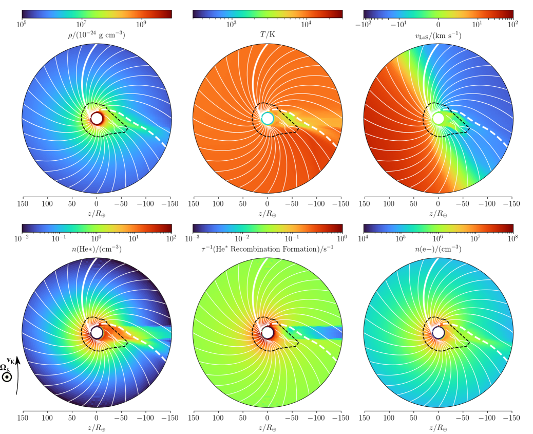
Figure 1: Profiles of the simulation for WASP-69b (fiducial model 69-0) in its quasi-steady-state. Stellar radiation comes from the left of the plot, and the orbital angular velocity $\mathbf{\Omega}_{\mathrm{K}}$ points out of the paper plane; the Keplerian motion of the plaent is upwards $\mathbf{v}_{\mathrm{K}}$. Colormaps show the mass density $\rho$ (upper left panel), temperature $T$ (upper middle), line-of-sight velocity $v_{\rm LoS}$ (upper right; the value is measured at mid-transit), $\mathrm{He}^{*}$ number density $n(\mathrm{He}^{*})$ (lower left), inverse timescale of recombination $\mathrm{He}^{*}$ formation (defined as formation rate normalized by $n(\mathrm{He}^{*})$; lower middle), and free electron number density $n(\mathrm{e}^{-})$ (lower right). White streamlines (projected to the orbital plane) are overlaid on each panel; two neighbor streamlines are separated in such a way that they are $\Delta\theta=\pi/16$ apart when they reach the outer radial boundary ($r=150~{}R_{\oplus}$). The heavy streamline are the reference lines on which the profiles are plotted in Figure 2). Black solid lines indicate the sonic surface.

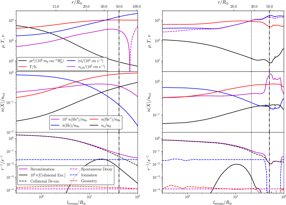
Figure 2: Key quantities of our fiducial model for WASP-69b (Model 69-0) along the two reference streamlines (plotted as the heavy streamlines in Figure 1). The top abscissa is the radial coordinate $r$ corresponding to the curve length along the streamline on the bottom abscissa. The top panels contain the profiles of scaled mass density $\rho r^{2}$, temperature $T$, velocity magnitude $|v|$ and the line-of-sight velocity $v_{\rm LoS}$. Dashed part of the $v_{\rm LoS}$ curve indicate negative values. The middle panels present the abundances of free electrons (relative to total hydrogen nucleus density $n_{\rm H}$) and helium in different forms (relative to the total helium nucleus density $n_{\rm He}$; note that $n(\mathrm{He}^{*})$ is multiplied by $10^{5}$ for clarity). Inverse timescales of $\mathrm{He}^{*}$ formation (in solid curves; note that the collisional excitation rate is multiplied by $10^{5}$) and destruction (in dashed curves) processes are shown in the bottom panels. In all panels, the vertical dotted line indicates the sonic critical point, and the vertical dash-dotted line shows the location of Roche radius.

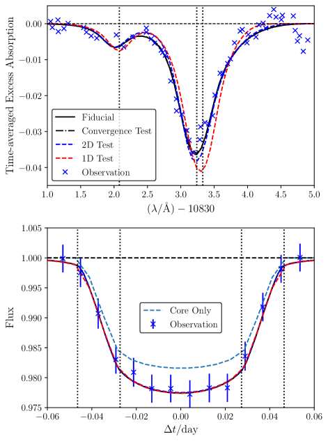
Figure 3: The observed and synthesized line profiles and light curves for WASP-69b. We include the results of our fiducial model (3D), 2D test, 1D test and a convergence test (same as fiducial but much higher grid resolution) (§2.1) as different line styles. Note that the curves for some test models overlap the fiducial curve and cannot be distinguished. The upper panel presents the time-averaged excess absorption transmission spectra or the resolved line profile (eq. 3; time-averaged from the end of ingress through the begin of egress). Three vertical dotted lines indicate the three central wavelengths of $\mathrm{He}^{*}$ triplet. The lower panel compares the synthesized light curve with the observations and a hypothetical planet that does not have any atmospheres. We have rebinned the light curve data in Nortmann et al. (2018). The four vertical dotted lines indicate the ingress and egress.

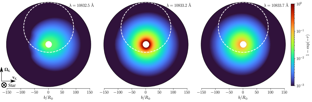
Figure 4: Extinction $[1-\exp(-\tau)]$ for Model 69-0 at three representative wavelengths $(\lambda/\text{\AA})\in\{10832.5,10833.2,10833.7\}$ near the $\mathrm{He}^{*}$ transitions. The profiles are measured at mid-transit (viz., all LoS are parallel to the star-planet line) and in a frame centered around the planet. The white dashed circles indicate the projected host star (with reported stellar radius and orbital inclination). The directions of orbit motion ($\mathbf{v}_{\mathrm{K}}$), orbital angular momentum vector ($\mathbf{\Omega}_{\mathrm{K}}$), and the direction to the host star are indicated at the lower-left corner of the whole figure.

Before analyzing our simulations, we ensured that quasi-steady states have been achieved. This usually involved running the simulations for many dynamical timescales, specifically we set $t_{\rm sim}\gtrsim 30~{}\tau_{\mathrm{dyn}}$. The dynamical timescale $\tau_{\mathrm{dyn}}$ is estimated by the sound crossing time of the Bondi radius:

$$\tau_{\mathrm{dyn}}\sim\dfrac{GM_{\rm p}}{c_{s}^{3}}\sim 1.2\times 10^{3}~{}\mathrm{s}\times\left(\dfrac{M_{p}}{10~{}M_{\oplus}}\right)\left(\dfrac{T}{10^{4}~{}\mathrm{K}}\right)^{-3/2}\ .$$ (4)

Here, $c_{s}$ is the sound speed. For a typical $T=10^{4}~{}\mathrm{K}$ outflow we see for WASP-69b, $\tau_{\mathrm{dyn}}\sim 10^{4}~{}\mathrm{s}$. Moreover, we also check explicitly if the simulation has settled down to a quasi-steady state by comparing key hydrodynamic/thermodynamic properties in neighboring dump files.

Our fiducial model for WASP-69b shows clear signs of a photoevaporative outflow. In Figure 1, we show 2D slices of the density, temperature and LOS velocity distributions of our 3D simulations looking down the North pole of the planet. We see a $T\gtrsim 10^{4}~{}\mathrm{K}$ hot ionized supersonic outflow originating at a wind base of $r\simeq 13~{}R_{\oplus}$ which eventually accelerates to $\sim 23~{}\mathrm{km}~{}\mathrm{s}^{-1}$ when leaving the domain of our simulation. This outflow disperses the planet atmosphere at a mass-loss rate of $\dot{M}\simeq 5.5\times 10^{-10}~{}M_{\oplus}~{}\mathrm{yr}^{-1}$. Since we assumed a constant high energy radiation output from the host star, the mass-loss rates and the hydrodynamic/thermodynamic profiles remain nearly constant after reaching the quasi-steady state. We also note that we did not put in any stellar wind from the host star, as the current wind-less model fits the data reasonably well and is preferred by Occam’s Razor. However in a companion paper on WASP-107 we will show that stellar winds may generate Kelvin-Helmholtz instability that leads to fluctuations of a photoevporative outflow.

Which mechanisms control the population of the $\mathrm{He}^{*}$ state? The bottom row in Figure 2 compares the rates of different (de-)population processes along the two particular streamlines (thickened curves in Figure 1). We compute the rate of ionization, recombination, spontaneous decay, collisional excitation and de-excitation as well as an advection attenuation term $|\mathbf{v}\cdot\nabla n(\mathrm{He}^{*})|$. Along the representative streamline presented by the left column, the abundance of $\mathrm{He}^{*}$ is determined by the relatively stiff balance between the recombination ($\mathrm{He}^{+}+\mathrm{e}^{-}\rightarrow\mathrm{He}^{*}$) and the collisional de-excitation at small radii $\lesssim 30~{}R_{\oplus}$. As expected these two processes are efficient at higher densities consistent with the law of mass action. Photoionization of $\mathrm{He}^{*}$ by soft FUV starts to take over the destruction channel of $\mathrm{He}^{*}$ where the density of free electrons declines at higher altitudes. The other channels have negligible importance: e.g. collisional excitation from $1^{1}$S to the metastable state is more than five orders of magnitude slower than recombination. On the right column of Figure 2, we show an interesting streamline that crosses in the shadow of the planet. The number density of $\mathrm{He}^{*}$ soars in the shadow because the photoionization of $\mathrm{He}^{*}$ by soft FUV vanishes here.

Beneath the base of the photoevaporative outflow ($r\lesssim 13~{}R_{\oplus}$), the temperature gradient between the day-side and the night-side generates a slow ”zonal” circulation ($\sim 0.1~{}\mathrm{km}~{}\mathrm{s}^{-1}$). However, this region has little observational effect on the overall $\mathrm{He*}^{*}$ observables which are mostly controlled by the much more extended low density regions of the outflowing atmosphere. We will return to this point shortly. Moving to higher altitude, this day-night advection continues, amounting to a $2-3\mathrm{km}~{}\mathrm{s}^{-1}$ blueshift at about $20-40~{}R_{\oplus}$. Going further away from the planet, the Coriolis effect starts to shape the outflow streamlines into spiral curves resulting in blueshifts on the leading edge and redshifts on the trailing edge. Considering that the outflow is still primarily radial, increments in the latitudinal velocity $|\Delta v_{\theta}|$ after traveling through a radial distance $\Delta r$ can be estimated by,

$$\begin{split}\Delta v_{\theta}\sim&~{}2\cos\phi\ \Omega_{\mathrm{K}}\int\mathrm{d}t\ v_{r}\simeq 2\cos\phi\ \Omega_{\mathrm{K}}\Delta r\\ \simeq&~{}2.3~{}\mathrm{km}~{}\mathrm{s}^{-1}\ \cos\phi\ \left(\dfrac{M_{*}}{M_{\odot}}\right)^{1/2}\\ &\times\left(\dfrac{a}{0.05~{}\mathrm{AU}}\right)^{-3/2}\left(\dfrac{\Delta r}{10~{}R_{\oplus}}\right)\ .\end{split}$$ (5)

This estimation is confirmed by the velocity profile in the top panels of Figure 2: if we compare the values at $r\simeq 40~{}R_{\oplus}$ and $r\simeq 100~{}R_{\oplus}$, the difference in $v_{\rm LoS}$ (approximately equals to $v_{\theta}$ for this streamline) is $\Delta v_{\rm LoS}\sim 11~{}\mathrm{km}~{}\mathrm{s}^{-1}$, and eq. (5) yields $\sim 10.8~{}\mathrm{km}~{}\mathrm{s}^{-1}$. This effect re-distributes $\mathrm{He}^{*}$ atoms in the velocity space and broadens the observed $\mathrm{He}^{*}$ line profiles as we will see shortly.

3.2 Comparison with Observations

Figure 3 shows our synthetic observations of both the line profiles and light curves of WASP-69b (Nortmann et al., 2018; Vissapragada et al., 2020). We have binned the light curve data from Vissapragada et al. (2020) for better clarity and the uncertainty represents the standard deviation within each phase bin. Our fiducial model of WASP-69 seems to fit both the spectroscopic and photometric observations well simultaneously. In particular, the synthetic line profile reproduced the subtle blueshift of the peak absorption, the overall line depth, and the relative ratio between the lines of this triplet. Numerically, Nortmann et al. (2018) reported a net blueshift of $-3.58\pm 0.23~{}\mathrm{km}~{}\mathrm{s}^{-1}$. This blueshift was based on fitting Gaussians to the observed line profiles; however, as we argued in the previous section, kinematic shift of the outflow introduces significant distortion of the spectral shape. Instead of fitting Gaussian to our line profile, we compared our simulations directly to the line profile itself which shows great agreement. We also use a different way to measure the blueshift: we report the blueshift of the peak absorption relative to a line-ratio-weighted average of the rest-frame line center for the two longer wavelength transistions that are usually blended together.

Nortmann et al. (2018) hinted at the possibility of a comet-like tail trailing behind WASP-69b. The basis of their suggestion is that additional $\mathrm{He}^{*}$ absorption can still be seen $\sim 20~{}\mathrm{min}$ after the nominal egress of the planet. The higher precision, better temporally sampled photometric data from Vissapragada et al. (2020) nontheless favors a symmetric transit. The symmetric transit shape (lower panel of Figure 3) does not support an extended comet-like tail. Our simulation seems to be more consistent with Vissapragada et al. (2020), the photoevaporative outflow of WASP-69b in our fiducial model is largely symmetric between the leading and trailing edge, hence it produces a more symmetric transit shape. We note that an extended comet-like tail will also introduce significant distortion to $\mathrm{He}^{*}$ line profile (see our Companion paper on WASP-107b for strong comet-like tail generated by strong stellar wind in that system). Here in the case of WASP-69b, our fiducial model produces a good fit the resolved line profile (Nortmann et al., 2018) while it does not need to invoke a prominent comet-like tail.

Another point we would like to emphasize is that a significant part of the $\mathrm{He}^{*}$ absorption for WASP-69 seems to be produced by an extended, optically thin ($\tau<1$) outer layer of the photoevaporative outflow. In Figure 4, we show the mid-transit extinction ($1-\exp^{-\tau}$) at three different wavelengths near the $\mathrm{He}^{*}$ transitions. The outer regions (10s of $R_{\oplus}$) contribute significantly to the overall extinction thanks to their extended area and the slow decrease of $\mathrm{He}^{*}$ number density in the outflow. Because of the unsaturated optical depth, the line ratios between the $\mathrm{He}^{*}$ triplet are close to $1:3:5$ i.e. their quantum degeneracies. More accurately, the line ratios are close to $1:8$ as the longer two lines are blended by kinematics and thermal broadening. This suggests that the line ratios between the $\mathrm{He}^{*}$ triplet can be a diagnostic of the number density in the outflow. If most of the $\mathrm{He}^{*}$ absorption is due to higher-density region where one of the line may saturate first, the line ratio will deviate from the quantum degeneracy ratio; this would tell us about the density of the outflow region in a model-independent way (see also discussions in Salz et al., 2018). This does not seem to be the case for WASP-69b, as most $\mathrm{He}^{*}$ absorption happens in lower density regions.

It is worth noting that, due to heavy computational cost of our 3D simulations, we could not afford to numerically fit the data with multiple simulation runs. Instead, our fiducial model serves as a validation our self-consistent 3D hydrodynamic simulations: with reasonable assumptions of the planetary/stellar properties and high energy SED, we can at least qualitatively reproduce the various $\mathrm{He}^{*}$ observables. That said, the degree to which our simulation agrees with observations is quite encouraging if not remarkable. After this validation of model, we stand at a position to perturb our fiducial model and investigate how the $\mathrm{He}^{*}$ observables are impacted by various factors that control the underlying photoevaporative outflow and $\mathrm{He}^{*}$ population in the following section.

4 Parametric Study

How do the photoevaporative outflow and the resultant $\mathrm{He}^{*}$ observables depend on key parameters in our simulations? In this section, we explore the impact of simulation dimensionality, XUV flux levels, host star spectral type, and planet surface gravity. This is done by perturbing validated fiducial model in these parameters. Before that, we did a further convergence test. We reran the fiducial model with a much finer simulation grid of $N_{\log r}\times N_{\theta}\times N_{\phi}=192\times 192\times 128$ (versus the fiducial model, $N_{\log r}\times N_{\theta}\times N_{\phi}=144\times 128\times 64$). The resultant $\mathrm{He}^{*}$ observables in the convergence test are almost identical (Figure 3) to the much faster fiducial model. This gives us confidence that the adopted spatial grid is fine enough to resolve the photoevaporative outflow on WASP-69b.

4.1 Dimensionality

To test how our model depends on the spatial dimensions of the simulations, we ran a 2D model with axisymmetry (about the $\phi$ axis i.e. $N_{\phi}=1$) while keep all system parameters the same as the fiducial model. The Coriolis forces is not captured in this 2D simulation while stellar gravity and orbital centrifugal forces are still involved. A reference 1D spherical symmetric model is also implemented using the $\theta=\pi/2,\phi=\pi/2$ radial line and removing the $\theta$ and $\phi$ components of the velocity.

Figure 3 compares the synthesized line profiles and light curves with all three dimensionality models. The 1D spherically symmetric model suffers from the loss of all non-radial kinematic information. It is clearly inconsistent with the observed line profile with no blueshift and limited kinematic broadening. The 2D axisymmetric test is able to capture the day-night advection. It shows good agreement with the observed line profile. The 3D fiducial model further modifies the line profile by including the Coriolis force. In this case of WASP-69b such a modification is quite subtle, which again testifies that the photoevaporative outflow on WASP-69b is largely symmetric between the leading and trailing edge. Again see our companion paper on WASP-107b for how this symmetry is broken by the inclusion of stellar winds.

The three models from 1D through 3D have almost identical equivalent width ($\langle W_{\lambda}\rangle\sim 3.1~{}\text{\AA}$) and light curves. This stresses the importance of spectrally resolving the $\mathrm{He}^{*}$ line profiles which are seen to vary the most between dimensions. The mass-loss rate are again quite similar between 3D and 2D models at about $\dot{M}\simeq 5.5\times 10^{-10}~{}M_{\oplus}~{}\mathrm{yr}^{-1}$. The mass-loss rate in our 1D model is off ($\dot{M}\simeq 6.9\times 10^{-10}~{}M_{\oplus}~{}\mathrm{yr}^{-1}$) because it assumes perfect spherical symmetry. However, the streamlines in Figure 1 are clearly non-radial. We also compare our results with that from a 1D isothermal model (Oklopčić & Hirata, 2018; Vissapragada et al., 2020) of

$9.5\times 10^{-10}~{}M_{\oplus}~{}\mathrm{yr}^{-1}$ ($\simeq 3\times 10^{-3}~{}M_{\rm Jup}~{}{\rm Gyr}^{-1}$) at an assumed temperature of 12000K. The results are in rough agreement with differences arising from more careful treatment of the hydrodynamics, thermodynamics and radiative transfer.

4.2 XUV Flux Intensity

Table 2: Radiation fluxes for different model host stars based on the fiducial model of WASP-69b

Star	$F_{20}$	$F_{15}$	$F_{13}$	$F_{13}$	$F_{13}$
type	$(2~{}\mathrm{eV})$	$(7~{}\mathrm{eV})$	$(12~{}\mathrm{eV})$	$(20~{}\mathrm{eV})$	$(40~{}\mathrm{eV})$
F	2.8	$1.6\times 10^{4}$	4.7	4.0	2.0
G	1.4	$8\times 10^{2}$	2.4	2.0	2.5
M	0.11	0.6	0.1	0.12	0.36

Note. — For simplicity, $F_{N}(h\nu)\equiv F(h\nu)/(10^{N}~{}{\rm cm}^{-2}{\rm s}^{-1})$, calibrated for the value at the planet orbit without any extinction.

Table 3: Results of various models, based on the fiducial model for WASP-69b

Model	Description	$\dot{M}$	$\langle W_{\lambda}\rangle$	$\Delta v_{\rm peak}^{\dagger}$	FWHM∗
		($10^{-9}~{}M_{\oplus}~{}\mathrm{yr}^{-1}$)	($10^{-2}~{}\text{\AA}$)	($\mathrm{km}~{}\mathrm{s}^{-1}$)	($\mathrm{km}~{}\mathrm{s}^{-1}$)
69-0	3D Fiducial	$0.55$	$3.16$	$-2.1$	$17.3$
69-0-2D	2D Test (fiducial parameters)	$0.56$	$3.10$	$-2.0$	$16.6$
69-0-1D	1D Test (fiducial parameters)	$0.69$	$3.14$	$0.07$	$16.2$
69-1	$10\times$ Flux for soft FUV ($h\nu=7~{}\mathrm{eV}$)	$0.61$	$1.75$	$-1.7$	$14.0$
69-2	$10\times$ Flux for LW ($h\nu=12~{}\mathrm{eV}$)	$0.56$	$3.18$	$-2.1$	$17.4$
69-3	$10\times$ Flux for soft EUV ($h\nu=20~{}\mathrm{eV}$)	$0.66$	$4.13$	$-2.4$	$24.2$
69-4	$10\times$ Flux for hard EUV ($h\nu=40~{}\mathrm{eV}$)	$2.50$	$5.62$	$-3.8$	$48.1$
69-5	$10\times$ Flux for X-ray ($h\nu=3~{}\mathrm{keV}$)	$0.55$	$3.12$	$-2.0$	$17.6$
69-6	$1/2$ Planet mass ($M_{\rm p}=41.3~{}M_{\oplus}$)	$0.93$	$4.25$	$-2.1$	$17.2$
69-F	Fiducial Model with F-type host	$0.70$	$0.04$	$-0.8$	$9.0$
69-G	Fiducial Model with G-type host	$0.64$	$0.51$	$-1.5$	$10.3$
69-M	Fiducial Model with M-type host	$0.05$	$1.40$	$-0.6$	$12.9$

Note. — The values are time averages taken over the last $15~{}\tau_{\mathrm{dyn}}$ of the simulations. Fluctuations are negligible for all models in the table.

$\dagger$: Shifts (postive values for redshifts and vice versa) of the right-hand-side peaks in the velocity space, compared to the line-ratio-averaged line center of $\lambda=10833.29~{}\text{\AA}$.

$*$: Full-width half-maximum of the longer-wavelength peak in the velocity space.

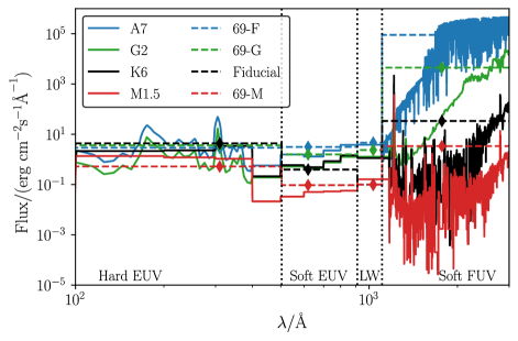
Figure 5: Spectral energy distributions of the incidenting high-energy photon fluxes, for the models with Type F, G, K and M host stars (Models 69-F, 69-G, fiducial model 69-0, and 69-M), presented in dashed lines. Diamonds overplotted on the dashed lines mark the exact energy of incident photons in the simulations (as represetatives of the corresponding energy bands; see §2.3). For reference, the model spectra of stellar spectral types A7, G2, K6 and M1.5 (based on the compilation in Oklopčić 2019) are shown in solid curves. Vertical dotted lines mark the boundary between different energy bands: “Hard EUV” for $h\nu>24.6~{}\mathrm{eV}$ photons that can ionize helium; “Soft EUV” for $13.6<(h\nu/\mathrm{eV})<24.6$ photons that can ionize hydrogen ; “LW” (short for Lyman-Werner) for $11.2<(h\nu/\mathrm{eV})<13.6$ photons that can photodissociate $\mathrm{H_{2}}$; “Soft FUV” for $h\nu<7~{}\mathrm{eV}$ photons.

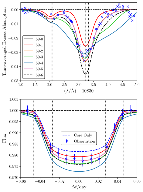
Figure 6: Similar to Figure 3 but for the models 69-0 through 69-6 in Table 3. The fiducial model 69-0 is also included for reference.

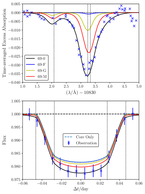
Figure 7: Similar to Figures 3 and 6, but presenting the models 69-F, 69-G, and 69-M for different host star spectral types in Table 3. Note fiducial model 69-0 is a K star.

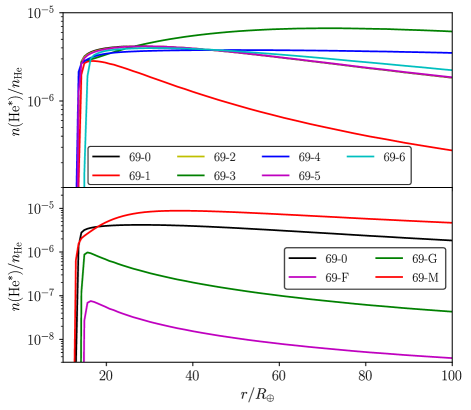
Figure 8: Relative abundance profiles of $\mathrm{He}^{*}$ (relateive to total helium nucleus density $n_{\rm He}$), measured along the radial line with $\theta=\pi/4$, $\phi=0$ in each simulation domain, for models described in Table 3. The upper panel shows models 69-0 and 69-1 through 69-6, while the lower panel specifically compares the results of different types of host stars (Model 69-0 for the K star WASP-69, and Models 69-F, 69-G and 69-M for F, G, M stars respectively).

Photoevaporative outflows are driven by high energy radiation from the host star. Moreover, the population of $\mathrm{He}^{*}$ states are also controlled by the critical balance high energy photons of different energy bins. We examine the impact of high energy radiation in each energy bin by perturbing the fidual model. The amount of high energy radiation a star outputs is variable depending on the evolution stage, activity and spectral types of the host star. Direct measurements are also lacking as the XUV measurements have to be performed in space. Therefore, in our Models 69-1 to 69-5 (soft FUV for 69-1, LW for 69-2, soft EUV for 69-3, hard EUV for 69-4, X-ray for 69-5), we bump up the flux level in each high energy bin by a whole order of magnitude to reflect the intrinsic variation in high energy flux level. We summarize key $\mathrm{He}^{*}$ observables in Table 3; we also show the synthetic line profiles and light curves in Figure 6 and the relative abundance of $\mathrm{He}^{*}$ as a function of radius in Figure 8.

The $\mathrm{He}^{*}$ line profiles are controlled mainly by the FUV (adverse effect) and the EUV bands (positive effect); the LW and X-ray bands only play minor roles under the “typical” host star conditions. More specifically, the relative abundance of $\mathrm{He}^{*}$ is suppressed by soft FUV because it photoionizes the $\mathrm{He}^{*}$ states, thus significantly reducing its population and the $\mathrm{He}^{*}$ absorption depth. In Model 69-1 ($\times 10$ soft FUV flux), the over-all mass-loss rate is enhanced by a few percent thanks to extra energy deposited into the atmosphere. However the stronger soft FUV flux significantly lowered the number density of $\mathrm{He}^{*}$ at a larger radial extent ($r\gtrsim 20~{}R_{\oplus}$). The $\mathrm{He}^{*}$ line profile depth and the light curve depth are both reduced by about a factor of two ($3.16~{}\text{\AA}$ to $1.75~{}\text{\AA}$). The line width also decreased (FWHM from $17.3~{}\text{\AA}$ down to $14.0~{}\text{\AA}$) because the high-altitude region with a higher velocity dispersion contribute less to the $\mathrm{He}^{*}$ extinction.

In Model 69-2 ($\times 10$ LW flux) the $\mathrm{He}^{*}$ observables are mostly unaltered from the fiducial model. This is because the LW band is intrinsically narrow thus only amount to a very small fraction of the overall high energy radiation flux. Moreover, most molecular H₂ are already dissociated at the $\sim 10^{4}$K in our simulations.

At higher EUV fluxes (Model 69-3 and 69-4), the much faster outflows not only bring more $\mathrm{He}^{*}$ into the exosphere but also spread them out in velocity space effectively broadening the line profiles. This confirms our earlier picture that EUV flux are most effective in driving photoevaporative outflows (WD18).

Finally, X-ray seems to play a secondary role in photoevaporation and $\mathrm{He}^{*}$ observables. Model 69-5 ($\times 10$ X-ray flux) has very similar observables as the fiducial model. Although X-rays photons are very energetic, they also have much smaller cross sections than EUV photons. As a result, X-ray penetrate deeper into the atmosphere where collisional processes and dust particles quickly convert the X-ray energies to infrared radiation that escapes easily. This limits the heating potential of X-ray. We reached a similar conclusion in WD18.

4.3 Host Spectral Type

Among the handful of reported $\mathrm{He}^{*}$ detections, 4 out of 6 are planets around K-type hosts (Spake et al., 2018; Venzmer & Bothmer, 2018; Allart et al., 2018; Salz et al., 2018; Ninan et al., 2020; Alonso-Floriano et al., 2019). Oklopčić (2019) confirmed that K-stars, at least in 1D isothermal models, may be at the sweet spot of FUV/EUV flux balance that best promote the $\mathrm{He}^{*}$ population and thus observablity. This section re-evaluates such a claim with our 3D hydrodynamic simulation coupled with self-consistent thermodynamics and radiative transfer.

We set up three additional models 69-F, 69-G, and 69-M, whose luminosities in different high energy bins emulate typical F-type, G-type, and M-type main-sequence stars based on the compilation of Oklopčić 2019. We remind the reader the fiducial model 69-0 has a K-star SED. The flux in each high energy bin is summarized in Table 2). Broadly speaking, F-type and G-type stars output similar levels of soft and hard EUV fluxes as K-type stars, however their FUV luminosities are significantly higher by a factor of $\sim 3000$ and $\sim 130$ respectively. For a typical M star, fluxes in all high energy bands are lower by about one order of magnitude.

$\mathrm{He}^{*}$ observables of these models are summarized in Table 3 for their mass-loss rates and a few key diagnostics etc. We show the line profiles and light curves in Figure 6 and the radial distribution of $\mathrm{He}^{*}$ in Figure 8. With a soft FUV flux $\sim 3000$ times higher than our fiducial model, F-type stars significantly suppress the population and observability of $\mathrm{He}^{*}$ with an equivalent width reduced by almost two orders of magnitude (3.16 to 0.04 Å). However, the mass loss rate of the photoevaporative outflow is similar to that of the fiducial model. Again, photoevaporation is driven mostly by EUV which have similar flux levels between F and K stars. On the other hand, for a typical M star host, whose higher energy flux levels are weaker in all bands, the mass loss rate is reduced by one order of magnitude. Nonetheless, the equivalent width of $\mathrm{He}^{*}$ in the transmission spectrum only decline by a factor of 2 (3.16 to 1.4 Å). Again this is because its much weaker soft FUV flux allows proportionally more $\mathrm{He}^{*}$ to exist in the outflow (Figure 8). G-star represents some middle ground, its $\sim 130$ times higher soft FUV flux suppress the equivalent width $\mathrm{He}^{*}$ by a factor of 6.

In summary, our findings suggest that K-star planet hosts are indeed favorable targets for $\mathrm{He}^{*}$ observations consistent with the suggestion of Oklopčić (2019). The high-energy SED, nonetheless, is expected to change significantly as a function of host star age and activity level. The suppression factor of $\mathrm{He}^{*}$ around G and M type stars are often only a factor of a few. We encourage observers to keep them in their target list particularly the young and active ones. We also predict that there will be more reports of $\mathrm{He}^{*}$ detection around G and M type hosts soon. Another important point we would like to stress is that the depth of $\mathrm{He}^{*}$ line profile can not be translated to the underlying mass loss rate without knowing the high energy SED of the host star. In other words, measuring the XUV SED of the host star directly is crucial for correctly interpreting the $\mathrm{He}^{*}$ observations.

4.4 Surface gravity

The mass-loss rate of photoevaporation depends quite strong on the depth of gravitational potential well of the planet. A shallower potential allows faster outflow with the same high energy irradiation. In Model 69-6 we adjusted the planet interior such that the planet mass is reduced by half while keeping the transit radius the same. This effectively lowers the surface gravity of the planet by a factor of two. The mass loss rate in Model 69-6 increases to $\dot{M}\simeq 9.3\times 10^{-10}~{}M_{\oplus}~{}\mathrm{yr}^{-1}$ which is $\sim 70~{}\%$ larger than the fiducial model. This larger mass loss rate can be decomposed into an increase in the terminal outflow velocity by $\sim 10~{}\%$ and an increase of the outflow density by $\sim 60~{}\%$.

The $\mathrm{He}^{*}$ line profile depth responds to this increase of mass loss rate sub-linearly. In Figure 6, the line profile has $\sim 40~{}\%$ larger depth than that in the fiducial model, while the equivalent width increases by about $\sim 30~{}\%$. However, the $\mathrm{He}^{*}$ line profile maintains a similar morphology with the peak velocity shift and the FWHM unchanged from the fiducial model (Table 3). In short, puffier, low surface gravity planets are more likely to undergo strong photoevaporative mass loss and should prove great target for $\mathrm{He}^{*}$ observations.

5 Variability and Stellar Flares

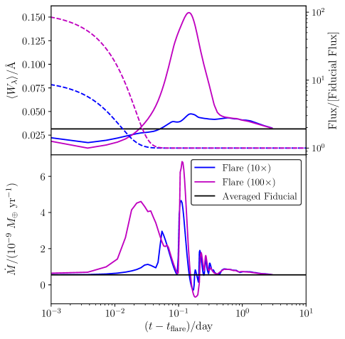
Figure 9: Temporal variation of the two models (based on Model 69-0) with flares that increase all high-energy radiation by $10$ and $100$ times uniformly (§5). The top panel shows the equivalent widths of the metastable helium absorption by solid curves. The two dashed lines, which should read the right ordinate, indicate the evolution of radiation fluxes in all energy bands. The mass-loss rates are shown in the lower panel. Time-averaged values for the fiducial model are also plotted for reference.

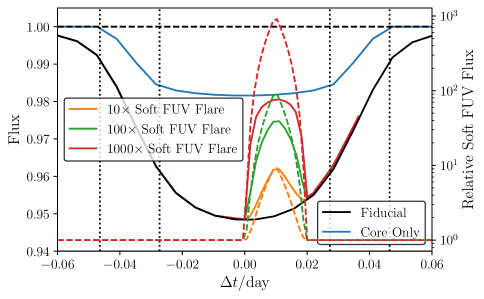
Figure 10: Slimilar to the lower panel of Figure 3, showing the light curves following soft-FUV-only flares that start at mid-transit ($\Delta t=0$) and terminating after $0.5~{}\mathrm{hr}$. Different flare intensities are indicated by colors. The light curves in solid lines should read the left ordinate, while the dashed lines are the flare shapes and should be read with the right ordinate. Soft-FUV-only destroys $\mathrm{He}^{*}$ while does not significantly perturb the photoevaporative outflow, thus only produces a decrease in $\mathrm{He}^{*}$ line depth that is seen in WASP-69b. Nontheless, we do not believe this is the explanation for the observed variability (see §5 for detail).

During one of the transit of WASP-69b in Nortmann et al. (2018), the $\mathrm{He}^{*}$ line profile experienced a $\sim 30\%$ drop in magnitude that lasted for about 20 minutes. This variability could well be instrumental in origin, but here we explore an alternative explanation that it is generated by a stellar flare on the host star.

Solar/stellar flares are associated with the surface magnetic activity of the host star. Their amplitudes can range below a percent to even orders of magnitude in extreme cases (“superflares” Günther et al., 2020, and references therein). The sudden rise of luminosity is often followed by exponential decays to nominal flux level on minutes or hours timescale. To investigate the consequences of flaring events on $\mathrm{He}^{*}$ observables, we first inject a simple flare model in which fluxes across all energy bands energy bands increase by a factor 10 and 100 times which then quickly decay to the quiescent state exponentially with a timescale of $500~{}\mathrm{s}$.

The temporal response of our fiducial model to these flares are shown in Figure 9. Independent of the energy injected, the common mode of response is as follows. Before the dynamics of the outflowing atmosphere can fully respond to the flares, the photoionization of $\mathrm{He}^{*}$ by soft FUV photons reduces the number density of $\mathrm{He}^{*}$ and cause a significant decrease in the equivalent width. It is only after the dynamical timescale $t-t_{\rm flare}\sim\tau_{\mathrm{dyn}}\sim$ hours that the flare-generated surge of photoevaporative mass-loss reach the higher altitudes where most of $\mathrm{He}^{*}$ absorption occurs. As a result, the equivalent width of $\mathrm{He}^{*}$ increases after the first hour or so and remains high for several hours. Looking at the mass-loss rate across the outer boundary of the simulation (lower panel of Figure 9), it experiences several oscillations on dynamical timescales as the systems response to the increased flux from the flare. The equivalent width (and other observables) however are the spatially integrated quantities, thus it effectively smears out most of these oscillations and has a much smoother variation (upper panel of Figure 9). Comparing with variability seen in WASP-69b (Nortmann et al., 2018), a flare that simultaneously raises all high energy radiation does not appear to be a good explanation. This is because it should be observed as a decrease followed by an increase of $\mathrm{He}^{*}$ absorption rather than the decrease only in the observations (Nortmann et al., 2018).

We therefore explore a different flare model in which only the soft FUV band. We do not have observational support that flares of this kind exist. We explore this rather contrived scenario just out of curiosity. Remember from §4.2 that the soft FUV primarily suppresses the $\mathrm{He}^{*}$ abundance by photoionization without significantly changing the overall kinematics. A soft-FUV-only flare may produce the observed decrease of $\mathrm{He}^{*}$ line depths. We setup three extra simulation runs, again based on the fiducial model of WASP-69b. We put in soft FUV flares ($10$, $100$ and $1000$ times the nominal value) that start at the middle of the transits and last for $30~{}\mathrm{min}$. In Figure 10, we can see that the light curves respond to these soft-FUV-only flares quickly. In order to reproduce the $\sim$30% variation, a soft FUV flare between $10-100\times$ the nominal level is required. This should be readily observable in the Ca ii H, K lines of the CARMENES spectra in Nortmann et al. (2018). Nevertheless, enhanced activity was not observed in the spectra during or preceding the observed light curve variation (private communications, Nortmann). Afterall, stellar flares do not seem to be a viable explanation of the temporal variability seen the $\mathrm{He}^{*}$ line profiles of Nortmann et al. (2018); instrumental effect is perhaps a better solution.

6 Summary

In this work, we simulate the ionized mass loss of close-in exoplanets and the metastable helium absorption during the planetary transit. We produce synthetic spectrally resolved line profiles and the light curves in a narrow filter band around the $\mathrm{He}^{*}$ transitions. Dynamics of such synthesis requires 3D hydrodynamic simulations of photoevaporating planetary atmospheres; non-equilibrium thermochemistry and ray-tracing radiative transfer are co-evolved with the hydrodynamics. The processes that populate and depopulate the metastable state of neutral helium are included in a thermochemical network and solved efficiently on GPUs.

With reasonable assumptions about the system parameters and high energy SED of WASP-69, we find a plausible model that launches a photoevaporative outflow with a mass-loss rate of $\dot{M}\simeq 5.5\times 10^{-10}~{}M_{\oplus}~{}\mathrm{yr}^{-1}$. The model yields a spectrum and a light curve that are in remarkable agreement with the observations in terms equivalent width, line-ratios, blueshift and line broadening (Nortmann et al., 2018; Vissapragada et al., 2020). Inside this outflow, metastable helium is formed almost solely by recombination. Its destruction is mainly due to collisional de-excitation at small radii where the density is high and photoionization by FUV photons at outer lower-density regions.

With this fiducial model of WASP-69b, we investigated how the photoevaporative outflow and $\mathrm{He}^{*}$ observables depend on various input parameters. 3D simulations are crucial for capturing the full hydrodynamics including Coriolis force and advection. These effects are needed for producing correct line profile including the line ratios, kinematic broadening and the overall blueshift. We found that EUV photons are most efficient in driving the photoevaporation dynamics and in producing $\mathrm{He}^{+}$ as the progenitors of recombination excitation of $\mathrm{He}^{*}$. The soft FUV photons that can ionize $\mathrm{He}^{*}$ often play an adverse effect on the $\mathrm{He}^{*}$ observability. X-ray photons, having much lower interaction cross section, are of secondary importance. Surface gravity also determines the effectiveness of photoevaporative outflows with puffier planets experiencing significantly stronger outflows, but the response of He* equivalent width is sub-linear.

K-stars are at a sweet spot of FUV/EUV balance that maximize the detectability of $\mathrm{He}^{*}$ lines. F or earlier type stars have excessive FUV fluxes that suppresses the $\mathrm{He}^{*}$ lines by orders of magnitude. G and M dwarfs represent a middle ground: $\mathrm{He}^{*}$ lines should still be observable particularly for the younger and more active ones. In any case, the depth $\mathrm{He}^{*}$ line profiles cannot be translated to a mass-loss rate without knowing the host star high energy SED.

We also investigated whether stellar flares could explain some of the temporal variability of WASP-69b (Nortmann et al., 2018). We found that a flare which enhances all high energy radiations initially suppresses $\mathrm{He}^{*}$ lines due to FUV fluxes ionizing the $\mathrm{He}^{*}$ before the whole system can adjust to higher mass-loss state after some dynamical timescales (usually hour-timescale). This characteristic shape is not consistent with the observed temporal variability of WASP-69b which only shows a decline of $\mathrm{He}^{*}$ line depth before returing to nominal levels. Stellar flares are unlikely to be the explanation for this type of variability.

This work is supported by the Center for Computational Astrophysics of the Flatiron Institute, and the Division of Geological and Planetary Sciences of the California Institute of Technology. L. Wang acknowledges the computing resources provided by the Simons Foundation and the San Diego Supercomputer Center. We thank our colleagues (alphabetical order): Philip Armitage, Zhuo Chen, Jeremy Goodman, Xiao Hu, Heather Knutson, Mordecai Mac-Low, Jessica Spake, Kengo Tomida, Songhu Wang, Andrew Youdin, and Michael Zhang, for helpful discussions and comments. We especially thank Shreyas Vissapragada for detailed suggestions and discussions.

Appendix A Cores and Interal Atmospheres of Model Planets

Gas giants like WASP-69b may have degenerate hydrogen and helium in their interior. We adopt the equations of state (EoS hereafter) tabulated by Miguel et al. (2016), which describe the behaviors of hydrogen and helium over wide ranges of pressure and temperature, from the degenerate states to ideal gases. Those tabulated EoS present the density and entropy of hydrogen and helium as functions of temperature and density. The combined EoS for a mixture of hydrogen and helium at a fixed atom number fraction $x_{\mathrm{H}}$ is given by solving the equation for $x_{p,\mathrm{H}}$ (the partial pressure of hydrogen),

$$\dfrac{m_{\mathrm{H}}x_{\mathrm{H}}}{m_{\mathrm{He}}(1-x_{\mathrm{H}})}=\dfrac{\rho_{\mathrm{H}}(p~{}x_{p,\mathrm{H}},T)}{\rho_{\mathrm{He}}[p(1-x_{p,\mathrm{H}}),T]}\ ,$$ (A1)

in which $p$ is the total pressure, $T$ is the temperature, $m_{\mathrm{H}}$ and $m_{\mathrm{He}}$ are the atomic masses of hydrogen and helium respectively, and $\rho_{\mathrm{H}},\ \rho_{\mathrm{He}}$ are interpolated from the EoS tables. The overall density then reads $\rho=\rho_{\mathrm{H}}+\rho_{\mathrm{He}}$. The entropy density $s$ of the materials is also calculated, so that we can obtain the adiabatic gradient,

$$\nabla_{\mathrm{ad}}\equiv\left(\dfrac{\partial\ln p}{\partial\ln T}\right)_{s}=-\dfrac{(\partial\ln s/\partial\ln p)_{T}}{(\partial\ln s/\partial\ln T)_{p}}\ .$$ (A2)

Note that the entropy of mixing does not affect these derivatives.

The spherical symmetric isentropic hydrostatics are calculated by solving a boundary value problem for the set of ordinary differential equations:

$$\dfrac{\mathrm{d}p}{\mathrm{d}r}=-\dfrac{GM\rho}{r^{2}}\ ,\quad\dfrac{\mathrm{d}M}{\mathrm{d}r}=4\pi r^{2}\rho\ ,\quad\dfrac{\mathrm{d}T}{\mathrm{d}r}=\nabla_{\mathrm{ad}}\left(\dfrac{T}{p}\right)\left(\dfrac{\mathrm{d}p}{\mathrm{d}r}\right)\ .$$ (A3)

where $M$ denotes the mass enclosed by radius $r$. Specifying the boundary conditions $(p_{c},\ T_{c})$ as the “eigenvalues”, we can integrate these ODEs from a the boundary of a dense solid core with radius $r_{c}$ and given mass $M_{c}$ up to the radiative-convective boundary $r=r_{\mathrm{rcb}}$. At $r_{\mathrm{rcb}}$ the temperature approaches the equilibrium temperature of the quasi-isothermal layer $T=T_{\mathrm{eq}}$. Thus the convective inner atmosphere is smoothly connected to an quasi-isothermal outer atmosphere whose density profile obeys ($\mu$ is the dimensional mean molecular mass),

$$\rho=\rho_{\mathrm{rcb}}\exp\left[\left(\dfrac{GM_{\mathrm{rcb}}\mu}{r_{\mathrm{rcb}}k_{\mathrm{B}}T_{\mathrm{eq}}}\right)\left(\dfrac{r_{\mathrm{rcb}}}{r}-1\right)\right]\ .$$ (A4)

The density profile is then used to calculate the effective transiting radius,

$$\langle r_{\mathrm{eff}}\rangle=\left\{\dfrac{1}{\pi}\int_{0}^{r_{\rm cut}}\mathrm{d}b\ 2\pi b\left[1-\mathrm{e}^{-\tau(b)}\right]\right\}^{1/2}\ ,$$ (A5)

where $r_{\rm cut}$ is an arbitrary cutoff size (to calculate the effective transiting radius in the broad optical band, we use $r_{\rm cut}=100~{}R_{\oplus}$), $\tau(b)$ is the optical depth along the LoS at impact parameter $b$,

$$\tau(b)\equiv\int_{-r_{\rm cut}}^{r_{\rm cut}}\mathrm{d}z\ \sigma n|_{r=\sqrt{b^{2}+z^{2}}}\ ,$$ (A6)

$n$ is the number density of the extinction particle, and $\sigma$ is the extinction cross section per particle. The eigenvalues $(p_{c},\ T_{c})$ are searched iteratively until both $M_{\mathrm{rcb}}$ and $\langle r_{\mathrm{eff}}\rangle$ match the observed the mass $M_{\rm p}$ and optical transiting radius $R_{\rm p}$ of the planet being simulated. In all models discussed in this paper, for simplicity, we assume that there is no rocky cores $r_{c}=0$, $M_{c}=0$. This assumption hardly affects the properties of the upper atmosphere. We also use $\kappa$ of the Thomson scattering to estimate calculate $\langle r_{\mathrm{eff}}\rangle$. We have also tested other plausible values of opacity (e.g. the optical $\kappa$ for $r_{\mathrm{dust}}=5~{}\text{\AA}$ very small grains with $10^{-4}$ dust-to-gas mass ratio), and the $\langle r_{\mathrm{eff}}\rangle$ varies by only $\sim 2\%$ under the same boundary conditions. Again the specific choice of opacity hardly affects the upper atmosphere.

References

- Allart et al. (2018) Allart, R., Bourrier, V., Lovis, C., et al. 2018, Science, 362, 1384, doi: 10.1126/science.aat5879
- Alonso-Floriano et al. (2019) Alonso-Floriano, F. J., Snellen, I. A. G., Czesla, S., et al. 2019, A&A, 629, A110, doi: 10.1051/0004-6361/201935979
- Anderson et al. (2014) Anderson, D. R., Collier Cameron, A., Delrez, L., et al. 2014, MNRAS, 445, 1114, doi: 10.1093/mnras/stu1737
- Drake (2006) Drake, G. 2006, High Precision Calculations for Helium (Springer Science+Business Media, Inc., New York), 199
- Drake (1971) Drake, G. W. 1971, Phys. Rev. A, 3, 908, doi: 10.1103/PhysRevA.3.908
- Edwards et al. (2003) Edwards, S., Fischer, W., Kwan, J., Hillenbrand , L., & Dupree, A. K. 2003, ApJ, 599, L41, doi: 10.1086/381077
- Ehrenreich et al. (2015) Ehrenreich, D., Bourrier, V., Wheatley, P. J., et al. 2015, Nature, 522, 459, doi: 10.1038/nature14501
- France et al. (2016) France, K., Loyd, R. O. P., Youngblood, A., et al. 2016, ApJ, 820, 89, doi: 10.3847/0004-637X/820/2/89
- Fulton et al. (2017) Fulton, B. J., Petigura, E. A., Howard, A. W., et al. 2017, AJ, 154, 109, doi: 10.3847/1538-3881/aa80eb
- Ginzburg et al. (2016) Ginzburg, S., Schlichting, H. E., & Sari, R. 2016, ApJ, 825, 29, doi: 10.3847/0004-637X/825/1/29
- Ginzburg et al. (2018) —. 2018, MNRAS, 476, 759, doi: 10.1093/mnras/sty290
- Gudel (1992) Gudel, M. 1992, A&A, 264, L31
- Günther et al. (2020) Günther, M. N., Zhan, Z., Seager, S., et al. 2020, AJ, 159, 60, doi: 10.3847/1538-3881/ab5d3a
- Gupta & Schlichting (2019) Gupta, A., & Schlichting, H. E. 2019, MNRAS, 487, 24, doi: 10.1093/mnras/stz1230
- Gupta & Schlichting (2020) —. 2020, MNRAS, 493, 792, doi: 10.1093/mnras/staa315
- Kirk et al. (2020) Kirk, J., Alam, M. K., López-Morales, M., & Zeng, L. 2020, AJ, 159, 115, doi: 10.3847/1538-3881/ab6e66
- Kulow et al. (2014) Kulow, J. R., France, K., Linsky, J., & Loyd, R. O. P. 2014, ApJ, 786, 132, doi: 10.1088/0004-637X/786/2/132
- Kwan et al. (2007) Kwan, J., Edwards, S., & Fischer, W. 2007, ApJ, 657, 897, doi: 10.1086/511057
- Lampón et al. (2020) Lampón, M., López-Puertas, M., Lara, L. M., et al. 2020, A&A, 636, A13, doi: 10.1051/0004-6361/201937175
- Lecavelier Des Etangs et al. (2010) Lecavelier Des Etangs, A., Ehrenreich, D., Vidal-Madjar, A., et al. 2010, A&A, 514, A72, doi: 10.1051/0004-6361/200913347
- Leighly et al. (2011) Leighly, K. M., Dietrich, M., & Barber, S. 2011, ApJ, 728, 94, doi: 10.1088/0004-637X/728/2/94
- Loyd et al. (2016) Loyd, R. O. P., France, K., Youngblood, A., et al. 2016, ApJ, 824, 102, doi: 10.3847/0004-637X/824/2/102
- Miguel et al. (2016) Miguel, Y., Guillot, T., & Fayon, L. 2016, A&A, 596, A114, doi: 10.1051/0004-6361/201629732
- Müller et al. (2019) Müller, B., Tauris, T. M., Heger, A., et al. 2019, MNRAS, 484, 3307, doi: 10.1093/mnras/stz216
- Nakamura et al. (2019) Nakamura, K., Takiwaki, T., & Kotake, K. 2019, PASJ, 71, 98, doi: 10.1093/pasj/psz080
- Ninan et al. (2020) Ninan, J. P., Stefansson, G., Mahadevan, S., et al. 2020, ApJ, 894, 97, doi: 10.3847/1538-4357/ab8559
- Nortmann et al. (2018) Nortmann, L., Pallé, E., Salz, M., et al. 2018, Science, 362, 1388, doi: 10.1126/science.aat5348
- Oklopčić (2019) Oklopčić, A. 2019, ApJ, 881, 133, doi: 10.3847/1538-4357/ab2f7f
- Oklopčić & Hirata (2018) Oklopčić, A., & Hirata, C. M. 2018, ApJ, 855, L11, doi: 10.3847/2041-8213/aaada9
- Owen & Wu (2013) Owen, J. E., & Wu, Y. 2013, ApJ, 775, 105, doi: 10.1088/0004-637X/775/2/105
- Owen & Wu (2016) —. 2016, ApJ, 817, 107, doi: 10.3847/0004-637X/817/2/107
- Owen & Wu (2017) —. 2017, ApJ, 847, 29, doi: 10.3847/1538-4357/aa890a
- Palle et al. (2020) Palle, E., Nortmann, L., Casasayas-Barris, N., et al. 2020, A&A, 638, A61, doi: 10.1051/0004-6361/202037719
- Rafikov (2006) Rafikov, R. R. 2006, ApJ, 648, 666, doi: 10.1086/505695
- Salz et al. (2018) Salz, M., Czesla, S., Schneider, P. C., et al. 2018, A&A, 620, A97, doi: 10.1051/0004-6361/201833694
- Seager & Sasselov (2000) Seager, S., & Sasselov, D. D. 2000, ApJ, 537, 916, doi: 10.1086/309088
- Spake et al. (2018) Spake, J. J., Sing, D. K., Evans, T. M., et al. 2018, Nature, 557, 68, doi: 10.1038/s41586-018-0067-5
- Stone et al. (2020) Stone, J. M., Tomida, K., White, C. J., & Felker, K. G. 2020, arXiv e-prints, arXiv:2005.06651. https://arxiv.org/abs/2005.06651
- Turner et al. (2016) Turner, J. D., Christie, D., Arras, P., Johnson, R. E., & Schmidt, C. 2016, MNRAS, 458, 3880, doi: 10.1093/mnras/stw556
- Venzmer & Bothmer (2018) Venzmer, M. S., & Bothmer, V. 2018, A&A, 611, A36, doi: 10.1051/0004-6361/201731831
- Vidal-Madjar et al. (2003) Vidal-Madjar, A., Lecavelier des Etangs, A., Désert, J. M., et al. 2003, Nature, 422, 143, doi: 10.1038/nature01448
- Vissapragada et al. (2020) Vissapragada, S., Knutson, H. A., Jovanovic, N., et al. 2020, AJ, 159, 278, doi: 10.3847/1538-3881/ab8e34
- Wahl et al. (2017) Wahl, S. M., Hubbard, W. B., Militzer, B., et al. 2017, Geophys. Res. Lett., 44, 4649, doi: 10.1002/2017GL073160
- Wang & Dai (2018) Wang, L., & Dai, F. 2018, ApJ, 860, 175, doi: 10.3847/1538-4357/aac1c0
- Youngblood et al. (2016) Youngblood, A., France, K., Loyd, R. O. P., et al. 2016, ApJ, 824, 101, doi: 10.3847/0004-637X/824/2/101
- Youngblood et al. (2017) —. 2017, ApJ, 843, 31, doi: 10.3847/1538-4357/aa76dd