Woods-Saxon-type of mean-field potentials with effective mass derived from the D1S Gogny force

Abstract

Analytic average mean-field potentials of the Fermi-function (Woods-Saxon) type for the whole nuclear chart with space-dependent effective mass are deduced from the D1S Gogny force. Those ready-for-use potentials are advertised as an alternative to other existing phenomenological mean-field potentials.

I Introduction

Phenomenological mean-field potentials of the Woods-Saxon type have been and are still in use for various purposes as, e.g., the low-cost evaluation of shell effects in the microscopic-macroscopic (Mic-Mac) calculation of the nuclear mass table. The latter approach counts still among the most accurate ones for the prediction of nuclear masses. However, those phenomenological mean-field potentials generally are given without effective mass, i.e., they have the bare mass $m$ as input. It is, however, well-known that the real part of the optical potential is energy-dependent and, therefore, an important physical ingredient is missing in present-day phenomenological mean field potentials.

This work intends to contribute to fill this gap. To this end we develop a phenomenological mean-field including effective mass, which to our knowledge does not exist in the previous literature. We deduce with semiclassical methods an analytic mean-field potential from the D1S Gogny force with space-dependent effective mass $m^{*}(r)$. Let us point out at this stage that the choice of the D1S Gogny force is not essential. We could have taken as well a Skyrme force with effective mass. The choice of the Gogny force is rather dictated because in the following paper we want to study its behavior in conjunction with the set up of a modified Mic-Mac model. Nevertheless, a possible advantage of using Gogny forces instead of the Skyrme ones is that in dynamical calculations, for example response function, one can treat higher momentum transfer whereas in the Skyrme case one is limited to low momenta, since it represents a quadratic expansion in momentum. Another possible advantage of using Gogny interactions may be the fact that these forces are designed such that they can describe simultaneously the particle-hole and the particle-particle channels, which allows one to describe succesfully open shell nuclei with the same interaction wihtout incresing the number of adjustable parameters. This is not the case of the Skyrme interactions, where the pairing field is computed with a different force. With our existing technology centelles98 ; gridnev98 ; soubbotin00 of solving Extended Thomas-Fermi (ETF) integro-differential equations with density functionals up to second-order $\hbar$ corrections using a given (finite-range) effective force, quantities such as mean-field potentials or effective masses can be readily computed. These potentials are subsequently accurately fitted by functions of the Fermi-type yielding analytic expressions ready for use. Since our approach has never been published in a coherent way, we will present in section II, the semiclassical theory which allows us to determine such mean-field potentials with effective mass. However, the reader not interested in the details of our approach, may directly read section III where we give the explicit analytical form of our potentials and effective masses. In a follow-up article, we will indeed show that this strategy can yield very accurate masses in a Mic-Mac calculation.

The paper is organized as follows. In the second section we review the ETF method with finite-range interactions and apply this formalism to the specific case of Gogny forces. The third section is devoted to the fits to generalized Fermi distributions of the results of the ETF calculations, i.e., neutron and proton densities, central and spin-orbit single-particle potentials and effective masses. These fits provide a simple parametrization of the aforementioned quantities as functions of the mass ($A$) and atomic ($Z$) numbers. These parametrizations may be useful for applications where parametrized densities, single-particle potentials or effective masses are required. In the fourth section we discuss some results for energy calculations. Finally, our conclusions are given in the last section.

II The Extended Thomas-Fermi approximation with finite-range forces

The ETF approximation to the Hartree-Fock (HF) method for non-local forces was introduced and discussed in Refs.centelles98 ; gridnev98 ; soubbotin00 . This approximation is rather general and can be applied to any finite-range force. However, in this work we will apply this formalism to the particular case of the Gogny interaction decharge80 . Due to the general applicability of our approximation, and given that there are several parametrizations of the Gogny interaction available in the literature, we do not specify the precise force here. Only later we will specialize to the D1S force berger91 . In general, the Gogny-type of force decharge80 can be written as

$$V({\bf R},{\bf s})=\sum_{i=1}^{i=2}\left(W_{i}+B_{i}P^{\sigma}-H_{i}P^{\tau}-M_{i}P^{\sigma}P^{\tau}\right)v_{i}(s)$$

$$+\left[t_{3}\left(1+x_{3}P^{\sigma}\right)\rho^{\alpha}({\bf R})+iW_{0}\left(\hat{\sigma}_{1}+\hat{\sigma}_{2}\right)\cdot{\hat{\bf k}^{\dagger}}\times{\hat{\bf k}}\right]\delta\left({\bf s}\right)\,,$$

(1)

where $W_{i}$, $B_{i}$, $H_{i}$ and $M_{i}$ are the usual spin-isospin exchange strength parameters of the finite-range force and $v_{i}(s)=\exp(-s^{2}/\mu_{i}^{2})$ (i=1,2) are the Gaussian form factors. The second term in Eq. (1) is the zero-range density-dependent contribution and the last one corresponds to the spin-orbit interaction, which is also zero-range with a strength $W_{0}$ as in the case of Skyrme forces vautherin72 . In Eq.(1) ${\bf R}=({\bf r_{1}}+{\bf r_{2}})/2$ and ${\bf s}={\bf r_{1}}-{\bf r_{2}}$ are the center of mass and relative coordinates. In the spin-orbit term the quantity ${\hat{\bf k}}$ represents the relative momentum of the two nucleons, expressed as ${\hat{\bf k}}=(\nabla_{1}-\nabla_{2})/2i$.

The HF energy is calculated as the integral of the energy density ${\cal H}$, which can be split into its kinetic, nuclear, Coulomb and spin-orbit contributions. For a finite-range nuclear interaction we can write

$$E_{HF}=\int{\cal H}\,d{\bf R}=\int\left[{\cal H}_{kin}+{\cal H}^{nucl}_{dir}+{\cal H}^{nucl}_{exch}+{\cal H}^{nucl}_{z.range}+{\cal H}_{Coul}+{\cal H}_{s.o}\right]\,d{\bf R}\quad.$$ (2)

The key quantity for writing the different contributions to the energy density is the one-body density matrix, which, at HF level, is defined as

$$\rho\left({\bf R}+\frac{\bf s}{2},{\bf R}-\frac{\bf s}{2}\right)=\sum_{i=1}^{A}\phi_{i}^{*}\left({\bf r}\right)\phi_{i}\left({\bf r^{\prime}}\right)\,,$$ (3)

where $\phi_{i}\left({\bf r}\right)$ are the single-particle HF wavefunctions. From this density matrix the particle, kinetic energy and spin densities can be obtained as

$$\rho\left({\bf R}\right)=\left.\rho\left({\bf R},{\bf s}\right)\right|_{s=0}$$ (4)

$$\tau({\bf R})=\left.\left(\frac{1}{4}\Delta_{R}-\Delta_{s}\right)\rho\left({\bf R},{\bf s}\right)\right|_{s=0}\,,$$ (5)

and

$${\bf J}({\bf R})=\left.-i\left[{\bf\hat{\sigma}}\times\left(\frac{1}{2}{\bf\nabla_{R}}+{\bf\nabla_{s}}\right)\right]\rho\left({\bf R},{\bf s}\right)\right|_{s=0},$$ (6)

respectively.

The ETF approximation to the Hartree-Fock (HF) energy for non-local potentials consists of replacing the quantal HF density matrix by its semiclassical counterpart. The latter contains, in addition to the pure Thomas-Fermi (TF)($\hbar^{0}$) term, the corrective gradient contributions up to the order $\hbar^{2}$ and even beyond, if so desired. Here we will consider the corrective terms only up to the $\hbar^{2}$ order. In this approximation the ETF density matrix for each kind of particles, which was derived in Refs.centelles98 ; gridnev98 ; soubbotin00 , can be written as

$${\tilde{\rho}}\left({\bf R},s\right)=\frac{3j_{1}\left(k_{F}s\right)}{k_{F}s}\rho+\frac{s^{2}}{216}\Bigg{[}\left\{\left[\left(9-2k_{F}\frac{f_{k}}{f}-2k_{F}^{2}\frac{f_{kk}}{f}+k_{F}^{2}\frac{f_{k}^{2}}{f}\right)\frac{j_{1}\left(k_{F}s\right)}{k_{F}s}-4j_{0}\left(k_{F}s\right)\right]\frac{\left({\bf\nabla}\rho\right)^{2}}{\rho}\,-\right.$$

$$\left.\left[\left(18+6k_{F}\frac{f_{k}}{f}\right)\frac{j_{1}(k_{F}s)}{k_{F}s}-3j_{0}(k_{F}s)\right]\Delta\rho-\left[18\rho\frac{\Delta f}{f}+\left(18-6k_{F}\frac{f_{k}}{f}\right)\frac{{\bf\nabla}\rho\cdot{\bf\nabla}f}{f}+12k_{F}\frac{{\bf\nabla}\rho\cdot{\bf\nabla}f_{k}}{f}-9\rho\frac{\left({\bf\nabla}f\right)^{2}}{f}\right]\frac{j_{1}(k_{F}s)}{k_{F}s}\right\}$$

$$-\frac{m^{2}}{\hbar^{4}}\frac{\rho W^{2}}{f^{2}}s^{2}\frac{j_{1}(k_{F}s)}{k_{F}s}-\frac{im}{2\hbar^{2}}\frac{\rho}{f}\hat{\sigma}\cdot\left({\bf W}\times{\bf s}\right)\frac{3j_{1}(k_{F}s)}{k_{F}s}\Bigg{]}_{k=k_{F}}\,.$$ (7)

Notice that for the sake of brevity, the subscripts ‘$q$’ denoting particle type (neutron or proton) have been suppressed. Here, $k_{F}=\left(3\pi^{2}\rho({\bf R})\right)^{1/3}$ is the local Fermi momentum for each type of nucleons and $j_{0}(k_{F}s)$ and $j_{1}(k_{F}s)$ are the spherical Bessel functions of orders 0 and 1 respectively. The quantity $f=f({\bf R},k)$ in Eq. (7) is the inverse of the position and momentum-dependent effective mass, which at ETF-$\hbar^{2}$ level is defined as:

$$f_{q}\left({\bf R},k\right)=1+\frac{m}{\hbar^{2}k}\frac{\partial V^{nucl}_{exch,q,0}({\bf R},k)}{\partial k},$$ (8)

where $V^{nucl}_{exch,q,0}({\bf R},k)$ is the Wigner transform of the exchange potential at TF level, which is given by

$$V^{nucl}_{exch,q,0}({\bf R},k)=\sum_{i=1}^{i=2}\int\,d{\bf s}\,e^{-i{\bf k}\cdot{\bf s}}v_{i}(s)\left[X_{e1,i}\rho_{q}({\bf R})\frac{3j_{1}(k_{F_{q}}({\bf R})s)}{k_{F_{q}}({\bf R})s}+X_{e2,i}\rho_{q^{\prime}}({\bf R})\frac{3j_{1}(k_{F_{q^{\prime}}}({\bf R})s)}{k_{F_{q^{\prime}}}({\bf R})s}\right]\,,$$ (9)

where $q=n,p$ and $q^{\prime}=p,n$, respectively. In this equation the coefficients $X_{e1,i}=M_{i}+H_{i}/2-B_{i}-W_{i}/2$ and $X_{e2,i}=M_{i}+H_{i}/2$ are combinations of the strengths of the different exchange terms in Eq.(1). It is important to note that the function $f=f({\bf R},k)$ in Eq. (7) and its spatial derivatives $\nabla f\equiv\nabla_{R}f({\bf R},k)$ and $\Delta f\equiv\Delta_{R}f({\bf R},k)$, momentum derivatives $f_{k}\equiv f_{k}({\bf R},k)$ and $f_{kk}\equiv f_{kk}({\bf R},k)$ that represent the first and second derivatives of $f({\bf R},k)$ with respect to $k$, and mixed derivatives $\nabla f_{k}\equiv\nabla_{R}f_{k}({\bf R},k)$ are all them evaluated at $k=k_{F}$ after taking the corresponding derivative. This is indicated by the subscript in the rightmost bracket of Eq.(7). The last two terms in the density matrix (Eq. (7)) are the contributions due to the spin-orbit force, which can be obtained from the propagator including this interaction (see e.g. Ref.bartel82 ). These terms depend on the form-factor of the spin-orbit potential, which for each type of nucleons is given by:

$${\bf W}_{q}=\frac{1}{2}W_{0}\big{(}{\bf\nabla}\rho+{\bf\nabla}\rho_{q}\big{)}.$$ (10)

This ETF formalism is completely general for interactions with a finite-range central term, as for example the Gogny force given in Eq.(1). The impact of the finite-range part of the interaction on the density-matrix appears through the momentum and position-dependent effective mass defined in Eq.(8) and its momentum and spatial derivatives. More details about the derivation of the ETF density matrix (Eq. (7)) and its comparison with earlier density matrix expansions available in the literature negele72 ; campi78 can be found in Ref.soubbotin00 .

The explicit form of the semiclassical kinetic energy and spin densities at ETF level can now easily be derived from the density matrix (Eq. (7)) using Eqs.(5) and (6), respectively. The kinetic energy density is given by

$$\tau\left({\bf R}\right) = \left.\left(\frac{1}{4}\Delta_{R}-\Delta_{s}\right){\tilde{\rho}}\left({\bf R},s\right)\right|_{s=0}$$ (11)

$$= \frac{3}{5}k_{F}^{2}\rho+\frac{1}{12}\Delta\rho\left[4+\frac{2}{3}k_{F}\frac{f_{k}}{f}\right]$$

$$+ \frac{1}{36}\frac{\left({\bf\nabla}\rho\right)^{2}}{\rho}\left[1+\frac{2}{3}k_{F}\frac{f_{k}}{f}+\frac{2}{3}k_{F}^{2}\frac{f_{kk}}{f}-\frac{1}{3}k_{F}^{2}\frac{f_{k}^{2}}{f^{2}}\right]$$

$$+ \frac{1}{6}\frac{\rho}{f}\left[\Delta f-\frac{({\bf\nabla}f)^{2}}{2f}\right]+\frac{1}{6}\frac{{\bf\nabla}\rho\cdot{\bf\nabla}f}{f}\left[1-\frac{1}{3}k_{F}\frac{f_{k}}{f}\right]$$

$$+ \frac{1}{9}\frac{{\bf\nabla}\rho\cdot{\bf\nabla}f_{k}}{f}+\frac{1}{2}\left(\frac{2m}{\hbar^{2}}\right)^{2}\frac{\rho}{f^{2}}W^{2},$$

and the spin density at ETF level can be expressed as

$${\bf J}_{ETF} = -i\left.\mathrm{Tr}\left\{\left[\sigma\times\left(\frac{{\bf\nabla}_{R}}{2}+{\bf\nabla}_{s})\right)\right]\left(\frac{-im}{2\hbar^{2}}\right)\frac{\rho}{f}\left[\sigma\cdot({\bf W}\times{\bf s})\right]\right\}\frac{3j_{1}(k_{F}s)}{k_{F}s}\right|_{s=0}$$ (12)

$$= \left.-\frac{3m}{\hbar^{2}}\frac{\rho}{f}\left[{\bf\nabla_{s}}\times\left({\bf W}\times{\bf s}\right)\right]\frac{3j_{1}(k_{F}s)}{k_{F}s}\right|_{s=0}=-\frac{2m}{\hbar^{2}}\frac{\rho{\bf W}}{f}.$$

Therefore, we see that at ETF level both, the kinetic energy and spin densities, become functionals of the particle densities $\rho_{q}({\bf R})$ for neutrons and protons. It is worthwhile to note that in the kinetic energy density (Eq. (11)) finite-range effects are encoded through the inverse effective mass $f$ (Eq. (8)) and its derivatives with respect to the position and momentum. If the effective mass is independent of the momentum, as it is the case of the zero-range Skyrme forces vautherin72 , the kinetic energy reduces to the $\hbar^{2}$ expansion reported in brack85 whereas, if the effective mass is equal to the physical one, the kinetic energy density reduces to the well-known Weizsäcker term. The semiclassical kinetic energy and spin densities are used to calculate the different pieces entering in the energy density (Eq. (2)), which for Gogny interactions are reported in the Appendix 1. It is important to note that due to the structure of the ETF density matrix (Eq. (7)), the exchange energy can be written as the sum of a $\hbar^{0}$ (Slater) contribution, which corresponds to the exchange energy in infinite nuclear matter, plus a $\hbar^{2}$ contribution, which can be finally recast in terms of the neutron and proton densities and their gradients up to second order, as it is explained in detail in Appendix 1. Therefore, in the ETF approximation soubbotin00 , the exchange energy becomes a local functional of the particle densities, as also happens starting from the Negele-Vautherin or the Campi-Bouyssy expansions of the density matrix negele72 ; campi78 .

Taking into account the semiclassical kinetic energy and spin densities, the latter one used to compute the spin-orbit energy, the total HF energy (Eq. (2)) at ETF level, $E_{HF}^{ETF}$, can be finally recast as a functional of the neutron and proton densities only (see Appendix 1 for further details). Therefore to find the semiclassical energy and the density profiles of a nucleus, one shall solve the following set of coupled equations of motion for neutrons and protons:

$$\frac{\delta}{\delta\rho_{n}}\bigg{[}E_{HF}^{ETF}-\mu_{n}\int\rho_{n}({\bf R})d{\bf R}\bigg{]}=0$$ (13)

and

$$\frac{\delta}{\delta\rho_{p}}\bigg{[}E_{HF}^{ETF}-\mu_{p}\int\rho_{p}({\bf R})d{\bf R}\bigg{]}=0.$$ (14)

This set of coupled second-order non-linear integro-differential equations can be solved for the neutron and proton densities by using, for example, the imaginary time-step method (see for example centelles90 and references therein). The self-consistent solution of Eqs.(13) and (14) provides the semiclassical proton and neutron densities, $\rho_{n}$ and $\rho_{p}$ respectively, which correspond to the fully variational solution of the ETF HF energy. An application of this semiclassical ETF method using the D1 Gogny force was reported in Ref.gridnev98 .

However, in this work instead of solving the full variational equations (13) and (14), which give the proton and neutron densities numerically point by point, we perform a restricted variational minimization of the ETF HF energy (Eq. (2)) using trial neutron and proton densities of generalized Fermi type for a large set of nuclei along the whole periodic table. In a second step, we fit the parameters of the trial densities, i.e. radii and diffuseness, as functions of the atomic mass and charge numbers. The semiclassical ETF approximation to obtain density profiles and binding energies in a restricted variational method with trial densities has been employed quite often in the past together with Skyrme forces brack85 . A detailed comparison between the predictions of the ETF approach using trial densities and solving the full equations of motion in the case of Skyrme forces can be found in Ref.centelles90 . From this study the following conclusions are obtained. On the one hand, it turned out that the density profiles using trial densities nicely reproduce the fully variational ones. On the other hand, the energies derived through the restricted variational procedure lie very close to energies computed from the fully variational solutions of the equations of motion brack85 ; centelles90 .

It is known since long that the variational solution of $E_{HF}^{ETF}$ at $\hbar^{2}$ order including the spin-orbit contribution overbinds the nuclei and gives neutron and proton radii too small and a diffuseness too sharp as compared with the corresponding quantal HF results brack85 ; centelles90 . This fact is probably due to the truncation of the semiclassical expansion at second order. To try to simulate higher-order contributions, at least in the case of Skyrme interactions, Krivine and Treiner proposed to renormalize the $\hbar^{2}$ contribution to the kinetic energy treiner86 . Following this idea, we renormalize the $\hbar^{2}$ kinetic energy by a factor $\beta_{KT}$ to obtain a semiclassical energy of the nucleus ²⁰⁸Pb $\sim$$-$1625 MeV, such that, by adding a shell correction $\sim$$-$11 MeV, one gets a total energy close to the experimental value $\sim$$-$1636 MeV. This relatively small value of shell correction for ²⁰⁸Pb has been argued to be a robust “experimental” value (see, for example, MS.66 ; ZEL.67 ; BRA.72 ) of the shell correction.

A very efficient way of recovering quantal effects, which are absent in semiclassical approximations of ETF type, is, in the spirit of the Kohn-Sham scheme, to replace in the semiclassical energy density the ETF particle, kinetic energy and spin densities by the corresponding HF expressions (see for instance Refs.gridnev98 ; soubbotin00 ). Applying now the variational principle using the single-particle wave-functions $\phi$ and $\phi^{*}$ for each type of particles as functional variables, one can write the following set of coupled single-particle differential equations:

$$H_{q}\phi_{i}=\epsilon_{i}\phi_{i},$$ (15)

where the single-particle Hamiltonian $H_{q}$ reads

$$H_{q}=-{\bf\nabla}\frac{\hbar^{2}}{2m_{q}^{*}({\bf R})}{\bf\nabla}+U_{q}({\bf R})-i{\bf W}_{q}({\bf R})\cdot\left[{\bf\nabla}\times{\bf\sigma}\right]\,,$$ (16)

where the effective mass, the mean-field and the spin-orbit potential for each kind of nucleons are given by

$$\frac{\hbar^{2}}{2m_{q}^{*}(r)}=\frac{\delta{\cal H}}{\delta\tau_{q}}\quad U_{q}=\frac{\delta{\cal H}}{\delta\rho_{q}}\quad{\bf W}_{q}({\bf r})=\frac{\delta{\cal H}}{\delta{\bf J}_{q}}\,.$$ (17)

This HF method reported here was introduced formally in Ref.soubbotin03 through a quasi-local reduction of the non-local density functional theory and generalized later on to take into account pairing correlations krewald06 . Using this approximation one can solve the HF problem with finite-range interactions in coordinate space, if spherical symmetry is assumed, with the same simplicity as for the case of Skyrme forces. It is found that this reproduces extremely well the full HF or HFB calculations as it can be seen in Refs. soubbotin03 ; krewald06 ; behera16 .

III Numerical investigations

Our aim in this paper is twofold. On the one hand, we want to provide parametrized ETF densities, single-particle and spin-orbit potentials as well as the effective mass for both, neutron and protons, which average the corresponding HF values obtained by solving Eqs. (15)-(17) with the same interaction. To this end we use the D1S Gogny force berger91 , which has been extensively applied in different nuclear calculations (see, for example, d1s ). These fully quantal calculations at HF or HFB levels, however, are usually numerically expensive, because of the fact that the Gogny interactions are finite range interactions. Therefore, it is interesting and important to investigate the possibility of the existence of an accurate parametrization in terms of the mass and atomic numbers of different ETF quantities associated with the Gogny D1S interaction, which can be used without performing explicitly the more cumbersome HF or HFB calculations.

On the other hand, these parametrized single-particle potentials fitted in this work could be used profitably to compute the shell corrections and therefore to estimate, perturbatively, the HF energy without performing explicitly the full HF calculation. In particular, the parametrized potentials are a key ingredient to obtain the shell-corrections through the so-called Wigner-Kirkwood $\hbar$-expansion method bhagwat10 ; bhagwat12 and this will be used in the Microscopic-Macroscopic calculation of nuclear masses based on the Gogny interaction reported in the paper II. It is worth to point out that this perturbative calculation of the shell corrections using semiclassical mean-field potentials has been recently applied to describe the inner crust of neutron stars in the Wigner-Seitz approximation using Gogny forces mondal20 .

III.1 Neutron and proton densities

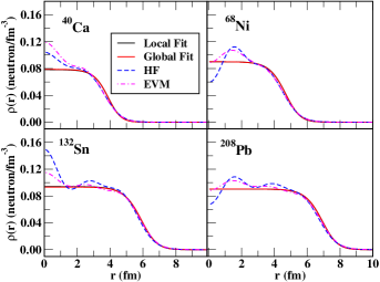
(a)  Neutron Density

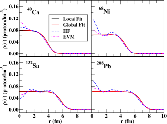
(b)  Proton Density

Figure 1: The nucleon density distributions for ⁴⁰Ca, ⁶⁸Ni, ¹³²Sn and ²⁰⁸Pb. The densities obtained by using the local and global parameters along with those from the Hartree-Fock calculations (denoted HF) and Expectation Value Method (denoted EVM, see section IV for further details) are displayed in the figure.

In this work the trial density profiles are chosen of the modified Fermi type. Explicitly,

$$\rho\left(r\right)~{}=~{}\rho_{o}\,g\left(r;R,a\right)$$ (18)

with

$$g\left(r;R,a\right)~{}=~{}f^{\nu}\left(r;R,a\right)$$ (19)

and

$$f\left(r;R,a\right)~{}=~{}\frac{1}{1+e^{\left(r-R\right)/a}},$$ (20)

where the half-density radius ($R$) and diffusivity ($a$) of each type of particles are the variational parameters, and $\rho_{o}$ is to be determined by the norm requirement. It is known that the exponent $\nu$ in (19) is practically unaffected by the minimization procedure brack85 , remaining always close to its starting value. Therefore, we fix values of these indices to be $\nu$ = 1.5 for neutrons and $\nu$ = 2.5 for protons. The reason for this choice will be discussed below in Section III.B.1.

Using these trial densities we minimize the ETF-HF total binding energies with a $\beta_{KT}$ factor equal to 1.9 and adding the direct and exchange (at Slater level) Coulomb contributions for a large set of 551 even-even nuclei (assumed to be spherical) covering a wide range of charge numbers, namely, from ²⁰Ne to ²³²Ds. With the aforementioned values of the exponents $\nu$ of the neutron and proton densities and of $\beta_{KT}$, the binding energy for ²⁰⁸Pb works out to be $\sim$1625 MeV, as discussed before.

As already mentioned, one of the aims of this work is to attempt a parametrization of the ETF self-consistent densities, mean fields and spin-orbit form factors computed with the Gogny D1S force, which give the average behaviour of the corresponding HF densities and fields. This in turn implies a systematization of the half-density radii and diffusivities as a function of $N$ and $Z$. The deformation can then be incorporated within this scheme by appropriately defining the distance function (see, for example, bhagwat10 ; bhagwat12 ). Thus, in order to study the systematics of the Fermi distribution parameters, spherical symmetry is assumed in the ETF calculations. The half-density radii and diffusivities thus obtained for the individual nucleus through a minimization process will be generically called ‘local’ parameters henceforth. The systematized radii and diffusivities as functions of $N$ and $Z$ will be termed as ‘global’ parameters. The corresponding results in the figures below have been labeled by the terms ‘local fit’ and ‘global fit’, respectively.

The kinetic energy densities, mean fields, spin-orbit potentials and the effective masses are obtained once the density parameters are optimized through a minimization process. These quantities will be termed as ‘exact’. These are then fitted to model form factors of the modified Fermi type for the each individual nucleus. The parameters thus obtained for the individual nucleus will be termed ‘local’ parameters, whereas the systematized radii and diffusivities as functions of $N$ and $Z$ will be termed as ‘global’ parameters. As in the case of the densities, the quantities obtained by using these parameters will be called ‘local fit’ and ‘global fit’ respectively.

The optimized half-density radii and diffusivity parameters for each kind of densities are modeled as

$$R^{(i)} = r_{1}^{(i)}\left(1+r_{2}^{(i)}\,I\right)A^{1/3}+r_{3}^{(i)}$$ (21)

$$a^{(i)} = a_{1}^{(i)}\left(1+a_{2}^{(i)}\,I\right)$$ (22)

where, $i$ = n (neutrons) or p (protons), $I=\left(N-Z\right)/A$ is the asymmetry parameter, and $r_{1,2,3}^{(i)}$ and $a_{1,2}^{(i)}$ are free parameters of the model. These are determined by using an implementation of the well-known Levenberg - Marquardt algorithm MAR.68 ; KEL.99 . The fits work out to be excellent, with rms residues being of the order of or even smaller than 10^-2 in all the cases. The explicit values of these parameters have been listed in Appendix 2.

In Figures 1(a) and 1(b) we display the point neutron and proton densities obtained from the minimization procedure discussed previously for the nuclei ⁴⁰Ca, ⁶⁸Ni, ¹³²Sn and ²⁰⁸Pb (‘local fit’) together with the densities provided by the global fit in comparison with the HF densities obtained by solving the set of Schrödinger equations (Eq. (15)). From these figures we also can see that the semiclassical densities nicely average the quantal oscillations and have a similar fall-off at the surface.

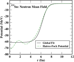
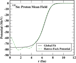
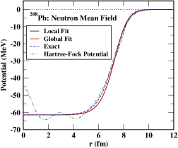
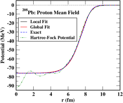
Figure 2: Calculated and fitted mean fields for ¹³²Sn and ²⁰⁸Pb compared with the corresponding HF potentials.

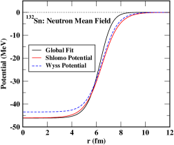
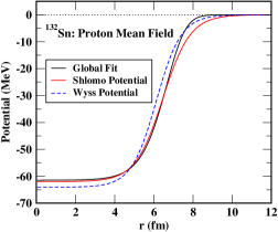
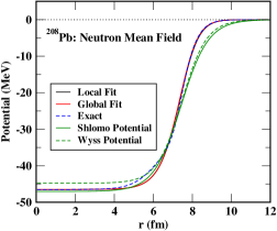
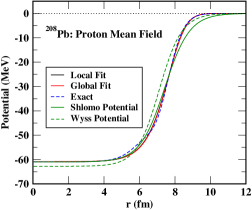
Figure 3: Calculated and fitted single-particle potentials with $m^{*}=m$ for ¹³²Sn and ²⁰⁸Pb compared with the phenomenological mean-fields of Refs.bhagwat10 ; bhagwat12 and shlomo92 .

III.2 Parametrized HF potentials and effective masses

We next investigate the possibility to parametrize the smoothly varying part of the HF neutron and proton mean-field, the spin-orbit potentials and the $r$-dependent effective masses employing the semiclassical ETF model described above. At HF level, the single-particle potential for each type of particles is obtained as the functional derivative of the energy density (Eq. (2)) with respect to the corresponding particle density (Eq. (17)). The corresponding ETF mean-field potentials, which we call ETF-HF potentials, are obtained by replacing in the HF potential the quantal kinetic energy and spin densities by the corresponding ETF counterparts, Eqs.(11) and (12), respectively. In an equivalent way, the semiclassical mean-field potential can also be derived from the ETF energy density functional using explicitly Eq.(44) of the Appendix and performing the variation with respect to the corresponding type of density, keeping the kinetic energy and spin densities as independent variables, as in the quantal case, and replacing them by the ETF expressions after variation.

Using the variational densities we can obtain all the quantities derived from the energy density functional, as for example the mean-field or the effective mass for each type of nucleons (which are the so-called ‘exact’ quantities discussed in the previous subsection). However, these ‘exact’ quantities are obtained numerically and are not easy to handle in a global way. We therefore undertake a second fit procedure, where we directly express these quantities by modified Woods-Saxon form factors whose parameters are adjusted to reproduce the ‘exact’ results. The parameters obtained from this local fit for a large set of nuclei are finally expressed as a function of the mass and atomic numbers, which allow to express the nuclear mean-fields, spin-orbit potentials and effective masses in a global form, which is ready for an easy and direct use as were before the phenomenological Woods-Saxon potentials (without effective mass) as given, e.g., by Shlomo shlomo92 .

III.2.1 Mean Field

Let us start with the mean-field. Specifically, we use:

$$V\left(r\right) = V_{o}f^{\nu}\left(r;R,a\right)$$ (23)

where the symbols have the same meaning as before. The indices $\nu$ for the neutronic and protonic mean fields have been taken to be 1.5 and 3.0 respectively. In the global fit the strengths, diffusivities and half-density radii are parametrized as:

$$V_{m}^{(i)} = V_{1}^{(i)}\left(1+V_{2}^{(i)}\,I\right)+V_{3}^{(i)}A^{1/3}$$ (24)

$$a_{m}^{(i)} = b_{1}^{(i)}\left(1+b_{2}^{(i)}\,I\right)$$ (25)

$$R_{m}^{(i)} = z_{1}^{(i)}\left(1+z_{2}^{(i)}\,I\right)A^{1/3}+z_{3}^{(i)}$$ (26)

As before, the index $i$ stands for neutrons (n) and protons (p). The quantities $V_{k}$, $b_{k}$ and $z_{k}$ are free parameters.

Here, we carry out two different fits of the neutron and proton single-particle potentials. In the first case, the optimal densities, deduced through the variational procedure discussed before, are used to obtain the single-particle HF potentials (ETF-HF potentials) for neutrons and protons as explained before. Those potentials are then fitted to modified Woods-Saxon form factors. These potentials can be directly compared with the true HF potentials obtained self-consistently.

In the second case, the contribution from the $r$-dependent effective mass is subsumed in the potential energy, thereby ensuring that only the constant ($r$-independent) bare mass appears in the kinetic energy operator. The motivation for this approach comes from the fact that the optical potentials, the phenomenological potentials used in the Mic-Mac calculations of nuclear masses, as well as the potentials fitted to reproduce the experimental observed single-particle states available in the literature have the effective mass equal to the bare mass. It should also be mentioned that the existing programs for this type of potentials work with bare mass and then would be complicated to include the effective mass in them, in particular in the deformed case. A few examples being, the potential proposed by Shlomo shlomo92 and the Wyss potential, used in our previous Mic-Mac calculations reported in Refs.bhagwat10 ; bhagwat12 . This scenario can also be easily simulated with our ETF approach. Notice that in the ETF energy density the contribution (Eq. (44)) can be split into a pure kinetic energy term with the bare mass (Eq. (35)) and a $\hbar^{2}$ contribution to the exchange energy (Eq. (43)). In this way, the effective mass contributions to the energy density have been subsumed in the potential part. This ensures that only the bare mass appears in the kinetic energy term (Eq. (35)) and that the total ETF energy remains unchanged. Within the strict semiclassical ETF approximation, the kinetic energy densities entering in the $\hbar^{2}$ exchange energy (Eq. (43)) have to be replaced by their semiclassical counterparts (Eq. (11)), which in turn are functionals of the particle densities. Only then one computes the neutron and proton single-particle potentials as functional derivatives of the potential energy density with respect to the density of each type of particles. We refer to the neutron and proton single-particle potentials obtained in this way as ETF phenomenological mean-field potentials.

For each single-particle potential, the strengths, the half-density radii and the diffusivities are systematized using the ansatz defined earlier (Eqs. (24)-(26)). The optimization of the parameters $V_{k}$, $b_{k}$ and $z_{k}$ is done separately in the two cases, by employing again the Levenberg-Marquardt algorithm. In both these cases, the fits are found to be good, with rms residues of the order of 10^-2. The explicit values of the parameters appearing above in both cases are listed in Appendix 2 under “Hartree-Fock mean field potentials” and “Phenomenological mean field potentials”, respectively. It is worth to remember here that the “Exact” mean-field potentials are complicated functions of the proton and neutron densities, which in turn depend on the exponent $\nu$. The “Exact” potentials are then fitted to generalized Fermi functions. We have chosen the exponents $\nu$ in the neutron and proton densities and mean-fields by a double optimization procedure in such a way that the fitted, local or global, single-particle potential for each type of particles reproduces as well as possible the “Exact” mean field. The fact that the proton mean field is slightly flatter at the bottom than the neutron mean field (see Figs. 2 and 3) is the reason why the proton exponents, for both density and mean field, are larger than the corresponding neutron exponents.

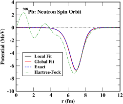
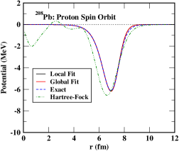
Figure 4: Calculated and fitted SO potentials for ²⁰⁸Pb compared with the corresponding HF results.

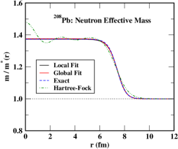
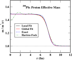
Figure 5: Calculated and fitted effective masses for ²⁰⁸Pb compared with the corresponding HF results.

As an example, the actual ETF-HF mean fields obtained using the variational densities (denoted by ‘exact’), as well as those obtained from the local and global parametrizations are plotted in the lower panel of Figure 2 for ²⁰⁸Pb. In the upper panel of the same figure we also show the ‘global fit’ and HF potentials for the nucleus ¹³²Sn. The single-particle potentials with $m^{*}=m$ are displayed in Figure (3). In the latter case, the phenomenological mean fields used in Refs. bhagwat10 ; bhagwat12 , labeled ‘Wyss Potential’ as well as the one reported by Shlomo shlomo92 , labeled ‘Shlomo Potential’, are also plotted for comparison. In the former case, as can be seen in Figure 2, the computed potentials nicely average out the HF potentials, which is as expected. Further, an excellent agreement between the different potentials for protons as well as neutrons is very clear from the above figure, indicating reliability of the fits achieved in this work. Regarding the phenomenological mean-field potentials, we see in the lower panel of Figure 3, that both, the local and the global fits, nicely reproduce the exact potential. In the upper panel of this Figure we show that for the nucleus ¹³²Sn the global fit of the ETF Gogny potential in the $m=m^{*}$ case qualitatively follows the trends of the Shlomo shlomo92 and Wyss bhagwat10 ; bhagwat12 phenomenological potentials. Similar results are found and the same comments hold for all the nuclei considered here. Actually, since the phenomenological mean field potentials of Refs. shlomo92 and bhagwat10 ; bhagwat12 are fitted to experiment, one can assume that a finite effective mass is also implicitly included in those potentials. Therefore, the closeness of the phenomenological potentials with the one from the Gogny force where we incorporate the effective mass into the local mean-field potential is not so astonishing.

III.2.2 Spin-Orbit Potential

The spin-orbit (SO) potential is studied next. Its form factor is given by Eq. (10), which we parametrize as

$$V_{so}\left(r\right) = \frac{\nu U_{so}}{a}\,g\left(f-1\right)$$ (27)

where, $f$ and $g$ are as defined above, and the other symbols have their usual meanings. Since the spin-orbit form factor (Eq. (10)) has been obtained by differentiating the neutron and proton densities, the indices $\nu$ for the spin orbit form factor have been chosen to be the same as those for the densities, namely, 1.5 and 2.5 for neutrons and protons, respectively.

The strengths, the diffusivities and the half-density radii of the spin-orbit potentials are parametrized as:

$$U_{so}^{(i)} = U_{1}^{(i)}\left(1+U_{2}^{(i)}\,I\right)+U_{3}^{(i)}A^{1/3}$$ (28)

$$a_{so}^{(i)} = b_{1}^{(i)}\left(1+b_{2}^{(i)}\,I\right)$$ (29)

$$R_{so}^{(i)} = z_{1}^{(i)}\left(1+z_{2}^{(i)}\,I\right)A^{1/3}$$ (30)

As an example, the neutron and proton SO potentials obtained from Eq.(10) using the variational densities (’Exact’ calculation) for the nucleus ²⁰⁸Pb as well as the corresponding local and global fits are displayed in Figure 4. The excellent agreement between the different potentials for protons as well as neutrons is very clear from the above figure. This observation for spin-orbit potentials is particularly important, since the accurate description of spin-orbit potential has a bearing on the ground-state masses as well.

For comparison, the HF values of the SO potentials are also plotted in the same graphs. The two profiles are quite similar to each other, but it can be seen that the SO potentials obtained from HF calculations have smaller radii, and they are a bit wider than the other potentials. This can be easily understood in the light of the density profiles, plotted in Figure (1). Notice that the HF and ETF densities have very similar slopes, but the HF densities tend to bulge slightly more in the surface region. Spin-orbit potential being proportional to the first derivative of the density profile, the ones obtained from HF and ETF densities are bound to be slightly different from each other, as is seen from Figure (1). It is important to point our that in order to reproduce the HF strength at the peak of the SO potentials, the spin-orbit strength has been taken $W_{0}=-105$ MeV instead of the original D1S value $W_{0}=-130$ MeV. This is due to the fact that although the ETF densities are in good agreement with the HF ones at the surface, their slopes are not exactly identical, which has a direct impact on the SO potential. As far as shell effects are dominated by the SO potential, we have renormalized the ETF prediction to remain as close as possible to the HF result for the SO potential.

III.2.3 Effective Mass

We next assume that the inverse of the effective mass (Eq. (11)) computed at $k=k_{F_{q}}(R)$ can be parametrized as:

$$\frac{m}{m^{*}(r)}-1=M_{o}\,g\left(r;R,a\right)$$ (31)

Here, the indices $\nu$ are chosen to be 1.5 and 2.5 respectively for neutrons and protons (same as those for densities). The strengths, half-density radii and diffusivity constants are parametrized as:

$$M_{o}^{(i)} = M_{1}^{(i)}\left(1+M_{i}^{(n)}\,I\right)$$ (32)

$$a_{em}^{(i)} = c_{1}^{(i)}\left(1+c_{2}^{(i)}\,I\right)$$ (33)

$$R_{em}^{(i)} = d_{1}^{(i)}\left(1+d_{2}^{(i)}\,I\right)+d_{3}^{(i)}$$ (34)

As in the case of the other quantities described above, the parameters $M_{1,2}$, $c_{1,2}$ and $d_{1,2,3}$ are taken to be free parameters, and are determined through a $\chi^{2}$ minimization process. As observed for the parameters of the mean field and the other quantities, the fits work out to be excellent, with typical rms deviation being of the order of 10^-2 or smaller. The explicit values of these parameters can be found in Appendix 2.

In Figure 5 we plot the quantity $m/m^{*}(r)$ for ²⁰⁸Pb, computed at ETF level using the variational densities (denoted by ‘Exact’), the corresponding local and global fits as well as the HF result. The results from the three approaches are almost indistinguishable from each other, indicating the good quality of the fits. It can be seen that the HF and ETF $m/m^{*}(r)$ ratios are very similar to each other. In fact, the ETF inverse effective mass nicely averages out that obtained from the HF calculations, as expected.

IV Energy calculations

Table 1: Total ground-state energies obtained by using the Hartree-Fock, Expectation Value Method and ETF approaches.

	Approach
Nucleus	HF	EVM	ETF
16O	-127.43	-126.08	-118.16
40Ca	-341.70	-339.34	-338.95
48Ca	-414.96	-413.57	-412.33
56Ni	-479.82	-476.36	-479.01
78Ni	-638.36	-636.12	-632.27
90Zr	-783.51	-781.63	-785.75
100Sn	-826.62	-822.66	-820.03
132Sn	-1100.72	-1097.68	-1089.09
208Pb	-1636.08	-1632.37	-1625.76

Table 2: The rms neutron and proton radii obtained by using the Hartree-Fock, Expectation Value Method and ETF approaches.

	$r_{n}$ (fm)			$r_{p}$ (fm)
	ETF	EVM	HF	ETF	EVM	HF
16O	2.54	2.57	2.67	2.51	2.65	2.70
40Ca	3.28	3.29	3.38	3.28	3.38	3.43
48Ca	3.54	3.61	3.60	3.40	3.45	3.45
56Ni	3.62	3.67	3.64	3.64	3.77	3.70
78Ni	4.14	4.21	4.18	3.91	3.97	3.90
90Zr	4.24	4.28	4.28	4.18	4.21	4.22
100Sn	4.33	4.36	4.34	4.38	4.48	4.42
132Sn	4.84	4.87	4.86	4.66	4.71	4.65
208Pb	5.56	5.58	5.58	5.44	5.48	5.43

The densities, mean fields and effective masses for neutrons and protons are the outcome of a restricted variational calculation of the semiclassical HF energy at ETF level. These energies computed for a set of doubly-magic nuclei are reported in Table 1. The HF energies, computed quantally as mentioned in Section II and explained in detail in soubbotin03 , are also given in the same Table. From the comparison between the HF and ETF results, we can see that for some nuclei the ETF energy over-binds the HF calculation. The semiclassical values go through the average of oscillating quantal energies. Therefore, it is natural that ETF sometimes gives higher, sometimes lower values than the quantal results.

According to the Strutinsky Energy theorem ring-schuck ; brack97 the HF energy splits in a large smoothly varying part plus a small oscillating shell correction that strongly depends on the considered nucleus. In our semiclassical calculation the smooth part of the energy is provided by the ETF value. A very efficient way to recover shell corrections is the so-called expectation value method (EVM) introduced by Bohigas and collaborators more than forty years ago bohigas76 . This method consists of including the shell corrections perturbatively on top of the semiclassical calculation by performing a single HF run using the semiclassical mean fields computed with the semiclassical densities. As stated in bohigas76 , the EVM treats basically the difference between the HF and ETF kinetic energies as a perturbation and allows to recover the shell effects missed in the semiclassical calculation. The EVM results obtained starting from our variational ETF calculation are also reported in Table 1. We can see that the EVM reproduces the full HF calculations accurately, the differences being always smaller than 1% in all the considered nuclei. The EVM can also reproduce the HF densities in a rather precise way as it can be seen in Fig. 1, where in addition to the ETF and HF densities, we also plot the densities generated by the EVM. The rms radii of densities of a set of spherical nuclei, along with those included in Fig. 1, are presented in Table 2, for all the three approaches (ETF, EVM and HF). As expected, the radii are quite close to each other in all the three cases.

V Summary and Conclusions

Extensive ETF calculations for a large number of even-even nuclei spanning the entire periodic table have been carried out using the Gogny D1S interaction, with the aim to deduce analytic average mean-field potentials from the D1S force with space-dependent effective mass, $m^{*}(r)$. In order to achieve this, the energy density at ETF level including second-order $\hbar$ corrections is minimized using trial neutron and proton densities parametrized as generalized Fermi distributions. The resulting densities are used to compute quantities such as mean-field, spin-orbit potentials and effective masses for each kind of particles. For each kind of nucleons the mean-field has been computed in two different ways. In the first one, the kinetic energy operator includes the space-dependent effective mass, whereas in the second one the effective mass contributions from the kinetic energy operator have been subsumed in the potential energy. The former approach has the advantage that the resulting analytical potentials are directly comparable with the Hartree-Fock potentials, whereas, the potentials obtained in the latter case, are similar to the phenomenological potentials available in the literature. We have demonstrated that the mean fields, spin-orbit potentials and position-dependent effective masses can be parametrized accurately using a simple modified Fermi function. It has been further shown that the parameters appearing in these Fermi-function forms can be systematized as functions of neutron and proton numbers up to very high degree of precision. The resulting semi-phenomenological potentials and other quantities are found to be very close to those obtained by the explicit ETF calculation with the D1S force. Our fitted densities, mean field potentials and effective masses are ready for use for any kind of nucleus, also the deformed ones albeit by suitable modifications of the distance function in the Woods-Saxon form factor. To our knowledge no such potential with effective mass can be found in the literature. The fitted neutron and proton densities may be useful in folding model calculations to obtain the nucleon-nucleus and nucleus-nucleus optical potentials bui15 . The knowledge of these fitted quantities is an advantage for accurate pairing calculations, where it is well known that effective masses play an important role decharge80 ; kucharek89 . Finally let us mention that these fitted mean-field potentials can directly be used to get accurate shell correction energies in Mic-Mac models for nuclear mass tables, as it will be shown in the follow-up paper.

Appendix 1: Additional details on the Extended Thomas-Fermi method with finite-range forces

Using the semiclassical particle, kinetic energy and spin densities (Eqs. (4-6)) given in Section II for each type of nucleons, the kinetic, zero-range, Coulomb and spin-orbit contributions to the ETF energy density functional can be easily obtained as

$${\cal H}_{kin}({\bf R})=\frac{\hbar^{2}}{2m}\bigg{(}\tau_{n}({\bf R})+\tau_{p}({\bf R})\bigg{)}$$ (35)

$${\cal H}^{nucl}_{z.range}({\bf R}) = \frac{t_{3}}{4}\rho^{\alpha}({\bf R})\bigg{[}(2+x_{3})\rho^{2}({\bf R})$$ (36)

$$- (2x_{3}+1)\bigg{(}\rho^{2}_{n}({\bf R})+\rho^{2}_{p}({\bf R})\bigg{)}\bigg{]}$$

$${\cal H}_{Coul}({\bf R}) = \frac{1}{2}\rho_{p}({\bf R})\int d{\bf R^{\prime}}\,\frac{\rho_{p}({\bf R-R^{\prime}})}{|{\bf R-R^{\prime}}|}$$ (37)

$$- \frac{3}{4}\left(\frac{3}{\pi}\right)^{1/3}\rho^{4/3}_{p}({\bf R})$$

$${\cal H}_{s.o}({\bf R}) = \frac{1}{2}W_{0}\bigg{[}\rho({\bf R}){\bf\nabla}\cdot{\bf J}({\bf R})$$ (38)

$$+ \rho_{n}({\bf R}){\bf\nabla}\cdot{\bf J}_{n}({\bf R})+\rho_{p}({\bf R}){\bf\nabla}\cdot{\bf J}_{p}({\bf R})\bigg{]}.$$

The contributions to the HF energy density due to the finite-range part of the force are collected in the direct and exchange terms. The direct energy reads:

$${\cal H}^{nucl}_{dir}({\bf R})=\frac{1}{2}\sum_{i=1}^{i=2}\int d{\bf R^{\prime}}v(|{\bf R-R^{\prime}}|)\bigg{[}X_{d1,i}\bigg{(}\rho_{n}({\bf R})\rho_{n}({\bf R^{\prime}})+\rho_{p}({\bf R})\rho_{p}({\bf R^{\prime}})\bigg{)}+X_{d2,i}\bigg{(}\rho_{n}({\bf R})\rho_{p}({\bf R^{\prime}})+\rho_{p}({\bf R})\rho_{n}({\bf R^{\prime}})\bigg{)}\bigg{]},$$ (39)

where $X_{d1,i}=W_{i}+B_{i}/2-H_{i}-M_{i}/2$ and $X_{d2,i}=W_{i}+B_{i}/2$, respectively.

The HF exchange energy density is given by

$${\cal H}_{HF}^{exch}=\frac{1}{2}\int V_{exch}^{nucl}({\bf R},{\bf s})\rho({\bf R},{\bf s})\,d{\bf R}\,d{\bf s}\,,$$ (40)

where ${\bf R}$ and ${\bf s}$ are the center-of-mass and relative coordinates, respectively, $\rho({\bf R},{\bf s})$ the ETF one-body density matrix (Eq. (7)) and $V_{exch}^{nucl}({\bf R},{\bf s})$ the exchange potential, which is defined as

$$V_{exch}^{nucl}({\bf R},{\bf s})=-v({\bf R},{\bf s})\rho({\bf R},{\bf s}),$$ (41)

where $v$(R,s) is the finite-range nucleon-nucleon interaction, which in the case of the Gogny interaction is given by the first term of Eq.(1). In the ETF approximation the exchange energy density consists of two terms. The first one corresponds to the Thomas-Fermi ($\hbar^{0}$) contribution, which in the Slater approach is given by

$${\cal H}^{nucl}_{exch,0}({\bf R})=\sum_{i=1}^{i=2}\int\,d{\bf s}\,v(s)\bigg{\{} \frac{1}{2} X_{e1,i}\bigg{[}\left(\rho_{n}({\bf R})\frac{3j_{1}(k_{F_{n}}({\bf R})s)}{k_{F_{n}}({\bf R})s}\right)^{2}+\left(\rho_{p}({\bf R})\frac{3j_{1}(k_{F_{p}}({\bf R})s)}{k_{F_{p}}({\bf R})s}\right)^{2}\bigg{]}$$ (42)

$$- X_{e2,i}\bigg{[}\rho_{n}({\bf R})\frac{3j_{1}(k_{F_{n}}({\bf R})s)}{k_{F_{n}}({\bf R})s}\rho_{p}({\bf R})\frac{3j_{1}(k_{F_{p}}({\bf R})s)}{k_{F_{p}}({\bf R})s}\bigg{]}\bigg{\}}.$$

The second term of the ETF exchange energy density, which contains the $\hbar^{2}$ corrections, is given by

$${\cal H}^{nucl}_{exch,2}({\bf R})=\sum_{q=n,p}\frac{\hbar^{2}}{2m}\bigg{\{} (f_{q}({\bf R})-1)\left(\tau_{q}({\bf R})-\frac{3}{5}k_{F_{q}}^{2}({\bf R})\rho_{q}({\bf R})-\frac{1}{4}\Delta\rho_{q}({\bf R})\right)$$ (43)

$$+ k_{F_{q}}({\bf R})f^{\prime}_{q}({\bf R})\bigg{[}\frac{1}{27}\frac{({\bf\nabla}\rho_{q}({\bf R}))^{2}}{\rho_{q}({\bf R})}-\frac{1}{36}\Delta\rho_{q}({\bf R})\bigg{]}\bigg{\}}.$$

The $\hbar^{2}$ contribution to the ETF exchange energy contains gradients of the neutron and proton densities and is explicitly connected with the nucleon-nucleon interaction through the effective mass (Eq. (8)) and its derivative with respect to the position and momentum $k$ computed at the Fermi momentum $k_{F}=(3\pi^{2}\rho({\bf R}))^{1/3}$. Notice that in the case of finite-range forces, such as the Gogny interaction, the nucleon effective mass only appears explicitly in the energy density when the $\hbar^{2}$ corrections are taken into account. In this case adding to the kinetic energy density (Eq. (35)) the second-order exchange energy density one can write:

$${\cal H}_{kin}({\bf R})+{\cal H}^{nucl}_{exch,2}({\bf R}) = \sum_{q=n,p}\frac{\hbar^{2}}{2m}f_{q}({\bf R})\tau_{q}({\bf R})+\sum_{q=n,p}\frac{\hbar^{2}}{2m}\bigg{\{}(1-f_{q}({\bf R}))\bigg{[}\frac{3}{5}k_{F_{q}}^{2}({\bf R})\rho_{q}({\bf R})+\frac{1}{4}\Delta\rho_{q}({\bf R})\bigg{]}$$ (44)

$$+k_{F_{q}}({\bf R})f^{\prime}_{q}({\bf R})\bigg{[}\frac{1}{27}\frac{({\bf\nabla}\rho_{q}({\bf R}))^{2}}{\rho_{q}({\bf R})}-\frac{1}{36}\Delta\rho_{q}({\bf R})\bigg{]}\bigg{\}}.$$

Appendix 2: Details of Fits

As mentioned in Section 3, here we present the details of parametrizations developed for the half-density radii, diffusivities, strength parameters, etc. As discussed there, the densities, mean fields, spin-orbit form factors, as well as effective masses are assumed to be of appropriately defined modified Woods-Saxon form.

1. Densities: We take,

   $$\rho^{(i)}=\rho^{(i)}_{o}\,g\left(r;R^{(i)},a^{(i)}\right)$$ (45)

   with $i$ = n or p (neutron or proton) and $\rho^{(i)}_{o}$ being determined from the normalization condition, and

   $$g\left(r;R^{(i)},a^{(i)}\right)=\left[f\left(r;R^{(i)},a^{(i)}\right)\right]^{\nu^{(i)}}$$ (46)

   with

   $$f\left(r;R^{(i)},a^{(i)}\right)=\frac{1}{1+e^{\left(r-R^{(i)}\right)/a^{(i)}}}$$ (47)

   The half-density radius and diffusivity parameters for neutrons and protons are parametrized as:

   $$R^{(n)} = 1.2031\left(1+0.0434\,I\right)A^{1/3}-0.0390$$ (48)

   $$R^{(p)} = 1.2559\left(1-0.1200\,I\right)A^{1/3}+0.1705$$ (49)

   $$a^{(n)} = 0.4619\left(1+0.8685\,I\right)$$ (50)

   $$a^{(p)} = 0.5656\left(1-0.3175\,I\right)$$ (51)

   here, $I=\left(N-Z\right)/A$ is the asymmetry parameter.

2. Hartree-Fock mean field potentials: With the definitions of $f$ and $g$ similar to those defined for the densities, the mean fields are assumed to be of the form:

   $$V^{(i)}(r)=V_{m}^{(i)}\left[f\left(r;R_{m}^{(i)},a_{m}^{(i)}\right)\right]^{\nu_{m}^{(i)}}$$ (52)

   where, the function $f$ being similar to the one defined for density distributions. The strength, half-density radius and diffusivity of neutrons and protons are parametrized as:

   $$V_{m}^{(n)} = -71.5435\left(1-0.3695\,I\right)+0.7552\,A^{1/3}$$ (53)

   $$V_{m}^{(p)} = -68.1452\left(1+0.4571\,I\right)-0.2045\,A^{1/3}$$ (54)

   $$R_{m}^{(n)} = 1.2251\left(1-0.1061\,I\right)A^{1/3}+0.4424$$ (55)

   $$R_{m}^{(p)} = 1.1899\left(1+0.1359\,I\right)A^{1/3}+1.2094$$ (56)

   $$a_{m}^{(n)} = 0.5587\left(1+0.4344\,I\right)$$ (57)

   $$a_{m}^{(p)} = 0.7636\left(1+0.3639\,I\right)$$ (58)

3. Phenomenological mean field potentials: With a definition similar to the Hartree-Fock mean field potentials, we have:

   $$V_{m}^{(n)} = -55.0321\left(1-0.4682\,I\right)+0.5261\,A^{1/3}$$ (59)

   $$V_{m}^{(p)} = -51.4006\left(1+0.6258\,I\right)-0.4422\,A^{1/3}$$ (60)

   $$R_{m}^{(n)} = 1.2310\left(1-0.1042\,I\right)A^{1/3}+0.4586$$ (61)

   $$R_{m}^{(p)} = 1.1801\left(1+0.1561\,I\right)A^{1/3}+1.2245$$ (62)

   $$a_{m}^{(n)} = 0.4876\left(1+0.7583\,I\right)$$ (63)

   $$a_{m}^{(p)} = 0.6776\left(1+0.2940\,I\right)$$ (64)

   where, the symbols have their usual meanings.

4. Spin-Orbit potential: The spin-orbit potential is assumed to be proportional to the derivative of modified Woods-Saxon form factor. Specifically, we take:

   $$V^{(i)}_{so}\left(r\right)=U_{so}^{(i)}\frac{d}{dr}\left\{\left[f\left(r;R_{so}^{(i)},a_{so}^{(i)}\right)\right]^{\nu_{so}^{(i)}}\right\}$$ (65)

   with the various quantities defined in a manner similar to those in the density distributions and mean fields. The strength, half-density radius and diffusivity for neutrons are protons are parametrized as:

   $$U_{so}^{(n)} = 13.1889\left(1+0.3072\,I\right)-0.1928\,A^{1/3}$$ (66)

   $$U_{so}^{(p)} = 13.0247\left(1-0.1840\,I\right)-0.2657\,A^{1/3}$$ (67)

   $$R_{so}^{(n)} = 1.2201\left(1-0.0014\,I\right)A^{1/3}-0.0752$$ (68)

   $$R_{so}^{(p)} = 1.2360\left(1-0.0452\,I\right)A^{1/3}+0.1840$$ (69)

   $$a_{so}^{(n)} = 0.4836\left(1+0.4937\,I\right)$$ (70)

   $$a_{so}^{(p)} = 0.5336\left(1+0.0966\,I\right)$$ (71)

   where, the symbols have their usual meanings.

5. Effective Mass: Finally, the $r$-dependent effective mass is parametrized through:

   $$\frac{m}{m^{*}(r)}-1=M^{(i)}_{o}\left[f\left(r;R_{em}^{(i)},a_{em}^{(i)}\right)\right]^{\nu_{em}^{(i)}}$$ (72)

   here, $m$ is the average nucleon mass, and the other symbols have their usual meanings. The strength, half-density radius and diffusivity for neutrons and protons are parametrized through:

   $$M_{o}^{(n)} = 0.4311\left(1-0.6033\,I\right)$$ (73)

   $$M_{o}^{(p)} = 0.4349\left(1+0.5772\,I\right)$$ (74)

   $$R_{em}^{(n)} = 1.2411\left(1-0.0827\,I\right)A^{1/3}+0.3806$$ (75)

   $$R_{em}^{(p)} = 1.1824\left(1+0.1636\,I\right)A^{1/3}+0.9225$$ (76)

   $$a_{em}^{(n)} = 0.3788\left(1+0.4480\,I\right)$$ (77)

   $$a_{em}^{(p)} = 0.4976\left(1+0.7033\,I\right)$$ (78)

   here, the symbols have their usual meanings.

The numerical values of the parameters here have been obtained through a $\chi^{2}$ minimization process, as discussed in Section 3 of this article.

For the sake of completeness, we summarize the indices ($\nu$) used for different quantities in Table (3).

Table 3: The indices $\nu$ appearing in the present parametrizations.

Index	Quantity where it appears	Value
$\nu^{(n)}$	Neutron density	1.5
$\nu^{(p)}$	Proton density	2.5
$\nu_{m}^{(n)}$	Neutron mean field	1.5
$\nu_{m}^{(p)}$	Proton mean field	3.0
$\nu_{so}^{(n)}$	Neutron spin-orbit potential	1.5
$\nu_{em}^{(p)}$	Proton spin-orbit potential	2.5
$\nu_{em}^{(n)}$	Neutron effective mass	1.5
$\nu_{so}^{(p)}$	Proton effective mass	2.5

- (1) M. Centelles, X. Viñas, M. Durand, P. Schuck and D. Von-Eiff, Ann. Phys. (N.Y.) 266, 207 (1998).
- (2) K. A. Gridnev, V. B. Soubbotin, X. Viñas and M. Centelles, Quantum Theory in honour of Vladimir A. Fock, Y. Novozhilov and V. Novozhilov (Eds.) Publishing Group of St.Petersburg University 1998, p.118; arXiv 1704.03858.
- (3) V. B. Soubbotin and X. Viñas, Nucl. Phys. A 665, 291 (2000).
- (4) J. Dechargé and D. Gogny, Phys. Rev. C 21, 1568 (1980).
- (5) J. F. Berger, M. Girod and D. Gogny, Comput. Phys. Commun. 63, 365 (1991).
- (6) D. Vautherin and D. M. Brink, Phys. Rev. C 5, 626 (1972).
- (7) J. Bartel and M. Vallieres, Phys. Lett. B 114, 303 (1982).
- (8) J. W. Negele and D. Vautherin, Phys. Rev. C 5, 1472 (1972); Phys. Rev. C 11, 1031 (1975).
- (9) X. Campi and A. Bouyssy, Phys. Lett. B 73, 263 (1978); Nukleonika 24, 1 (1979).
- (10) M. Brack, C. Guet and H.-B. Håkansson, Phys. Rep. 123, 275 (1985).
- (11) M. Centelles, M. Pi, X. Viñas, F. Garcias and M. Barranco, Nucl. Phys. A 510, 397 (1990).
- (12) J. Treiner and H. Krivine, Ann. Phys. (N.Y.) 170, 406 (1986).
- (13) W. D. Myers and W. J. Swiatecki, Proceedings of the Lysekil Symposium (1966), Ark. Fys. 36, 343 (1967).
- (14) N. Zeldes, A. Grill and A. Simievic, Mat. Fys. Skr. Dan. Vid. Selsk. 3, 1 (1967).
- (15) M. Brack, J. Damgaard, A. S. Jensen, H. C. Pauli, V. M. Strutinsky, and C. Y. Wong, Rev. Mod. Phys. 44, 320 (1972).
- (16) V. B. Soubbotin, V. I. Tselyaev and X. Viñas, Phys. Rev. C 67, 014324 (2003).
- (17) S. Krewald, V. B. Soubbotin, V. I. Tselyaev and X. Viñas, Phys. Rev. C 74, 064310 (2006).
- (18) B. Behera, X. Viñas, T. S. Routray, L. M. Robledo, M. Centelles and S. P. Pattnaik, J. Phys. G: Nucl. Part. Phys. 43, 045115 (2016).
- (19) CEA web page www-phynu.cea.fr.
- (20) A. Bhagwat, X. Viñas, M. Centelles, P. Schuck and R. Wyss, Phys. Rev. C 81, 044321 (2010).
- (21) A. Bhagwat, X. Viñas, M. Centelles, P. Schuck and R. Wyss, Phys. Rev. C 86, 044316 (2012).
- (22) C. Mondal, X. Viñas, M. Centelles and J. N. De, Phys. Rev. C 102, 015802 (2020).
- (23) D. W. Marquardt, J. Soc. Ind. Appl. Math. 11, 431 (1963).
- (24) C. T. Kelley, Iterative Methods for Optimization (SIAM, Philadelphia, 1999).
- (25) S. Shlomo, Nucl. Phys. A 539, 17 (1992).
- (26) A. J. Koning and J. P. Delaroche, Nucl. Phys. A 713, 231 (2003).
- (27) P. Ring and P. Schuck, The Nuclear Many-Body Problem (Springer-Verlag, Berlin, 1980).
- (28) M. Brack and R. K. Bhaduri, Semi-classical Physics (Addison-Wesley Publishing Co., 1997).
- (29) O. Bohigas, X. Campi, H. Krivine and J. Treiner, Phys. Lett. B 64, 381 (1976).
- (30) Doan Thi Loan, Biu Minh Loc and Dao T Khoa, Phys. Rev. C 92, 034304 (2015).
- (31) H. Kucharek, P.Ring and P. Schuck, Z. Phys. A 334, 119 (1989).