Corrected CBOW Performs as well as Skip-gram

Abstract

Mikolov et al. (2013a) observed that continuous bag-of-words (CBOW) word embeddings tend to underperform Skip-gram (SG) embeddings, and this finding has been reported in subsequent works. We find that these observations are driven not by fundamental differences in their training objectives, but more likely on faulty negative sampling CBOW implementations in popular libraries such as the official implementation, word2vec.c, and Gensim. We show that after correcting a bug in the CBOW gradient update, one can learn CBOW word embeddings that are fully competitive with SG on various intrinsic and extrinsic tasks, while being many times faster to train.

1 Introduction

Pre-trained word embeddings are a standard way to boost performance on many tasks of interest such as named-entity recognition (NER), where contextual word embeddings such as BERT (Devlin et al., 2019) are computationally expensive and may only yield marginal gains. Word2vec (Mikolov et al., 2013a) is a popular method for learning word embeddings because of its scalability and robust performance. There are two main Word2vec training objectives: (1) continuous bag-of-words (CBOW) that predicts the center word by averaging context embeddings, and (2) Skip-gram (SG) that predicts context words from the center word.

It has been frequently observed that while CBOW is fast to train, it lags behind SG in performance. This observation is made by the inventors of Word2vec themselves (Mikolov, 2013), and also independently in subsequent works (Pennington et al., 2014; Stratos et al., 2015). This result is surprising since the CBOW and SG objectives lead to very similar weight updates. This is also contrary to the enormous success of contextual word embeddings based on masked language modeling (MLM), as CBOW follows a rudimentary form of MLM (i.e., predicting a masked target word from a context window without any perturbation of the masked word).

In this work, we find that the performance discrepancy between CBOW and SG embeddings is founded less on theoretical differences in their training objectives but more on faulty CBOW implementations in standard libraries such as the official implementation word2vec.c (Mikolov et al., 2013b), Gensim (Řehůřek and Sojka, 2010) and fastText (Bojanowski et al., 2017). Specifically, we find that in these implementations, the gradient for source embeddings is incorrectly multiplied by the context window size, resulting in incorrect weight updates and inferior performance.

We make the following contributions. First, we show that our correct implementation of CBOW indeed yields word embeddings that are fully competitive with SG while being trained in less than a third of the time (e.g., with a single machine it takes less than 73 minutes to train CBOW embeddings on the entire Wikipedia corpus). We present experiments on intrinsic word similarity and analogy tasks, as well as extrinsic eval uations on the SST-2, QNLI, and MNLI tasks from the GLUE benchmark (Wang et al., 2018), and the CoNLL03 English named entity recognition task (Sang and De Meulder, 2003).

Second, we make our implementation, kōan, publicly available. With this implementation, it is possible to train 768-dimensional CBOW embeddings on one epoch of English C4 (Raffel et al., 2020) in 1.61 days on a single 16 CPU machine.

2 CBOW Implementation

The parameters of CBOW are two sets of word embeddings: “source-side” and “target-side” vectors $v_{w},v^{\prime}_{w}\in\mathbb{R}^{d}$ for every word type $w\in V$ in the vocabulary. A window of text in a corpus consists of a center word $w_{O}$ and context words $w_{1}\ldots w_{C}$. For instance, in the window the dog laughed, we have $w_{O}=\texttt{dog}$ and $w_{1}=\texttt{the}$ and $w_{2}=\texttt{laughed}$. Given a window of text, the CBOW loss is defined as:

$$v_{c} =\frac{1}{C}\sum_{j=1}^{C}v_{w_{j}}$$

$$\mathcal{L} =-\log\sigma({v^{\prime}_{w_{O}}}^{\top}v_{c})-\sum_{i=1}^{k}\log\sigma(-{v^{\prime}_{n_{i}}}^{\top}v_{c})$$

where $n_{1}\ldots n_{k}\in V$ are negative examples drawn iid from some noise distribution $P_{n}$ over $V$. The gradients of $\mathcal{L}$ with respect to the target ($v^{\prime}_{w_{O}}$), negative target ($v^{\prime}_{n_{i}}$), and average context source ($v_{c}$) embeddings are:

$$\frac{\partial\mathcal{L}}{\partial v^{\prime}_{w_{O}}}= (\sigma({v^{\prime}_{w_{O}}}^{\top}v_{c})-1)v_{c}$$

$$\frac{\partial\mathcal{L}}{\partial v^{\prime}_{n_{i}}}= \sigma({v^{\prime}_{n_{i}}}^{\top}v_{c})v_{c}$$

$$\frac{\partial\mathcal{L}}{\partial v_{c}}= (\sigma({v^{\prime}_{w_{O}}}^{\top}v_{c})-1)v^{\prime}_{w_{O}}+$$

$$\sum_{i=1}^{k}\sigma({v^{\prime}_{n_{i}}}^{\top}v_{c})v^{\prime}_{n_{i}}$$ (1)

and by the chain rule with respect to a source context embedding:

$$\frac{\partial\mathcal{L}}{\partial v_{w_{j}}}=\frac{1}{C}[ (\sigma({v^{\prime}_{w_{O}}}^{\top}v_{c})-1)v^{\prime}_{w_{O}}+$$

$$\sum_{i=1}^{k}\sigma({v^{\prime}_{n_{i}}}^{\top}v_{c})v^{\prime}_{n_{i}}]$$ (2)

However, the CBOW negative sampling implementations in word2vec.c , Gensim , and fastText incorrectly update each context vector, $v_{w_{j}}$, by Eq. (1), without normalizing by the number of context words, given in Eq. (2). In fact, this error has been pointed out in several Gensim issues as well as a fastText issue.

Why This Error Matters

Aside from being incorrect, this update matters for two reasons. First, in both Gensim and word2vec.c, the width of the context window is randomly sampled from ${1,\ldots,C_{\text{max}}}$ for every target word. This means that source embeddings which were averaged over wider context windows will experience a larger update than their contribution, relative to source embeddings averaged over narrower windows. Second, in the incorrect gradient, $\frac{\partial\mathcal{L}}{\partial v}$ is incorrectly scaled by $C$, while $\frac{\partial\mathcal{L}}{\partial v^{\prime}}$ is not; the correct stochastic gradient with respect to all embeddings actually points in a different direction than what was implemented in word2vec.c. Section 5 touches on both of these issues in more detail.

3 Experiments

We evaluated CBOW and SG embeddings under Gensim and our implementations (both corrected and original CBOW). Unless otherwise noted, we learn word embeddings on the entire Wikipedia corpus PTB sentence split and tokenized with default settings, where words occurring fewer than ten times were dropped. Training hyperparameters were held fixed for each set of embeddings: negative sampling rate 5, maximum context window of 5 words, number of training epochs 5, and embedding dimensionality 300 unless otherwise noted.

We found that the default initial learning rate in Gensim, 0.025, learned strong SG embeddings. However, we swept separately for CBOW initial learning rate for Gensim and our implementation. We swept over initial learning rate in $\{0.025,0.05,0.075,0.1\}$ selecting 0.025 to learn Gensim CBOW embeddings and 0.075 for corrected CBOW, to maximize average performance on the development fold (random partition of 50% of examples) of intrinsic evaluation tasks described in 3.1. We selected learning rate as this was a critical hyperparameter, and we found that CBOW embeddings learned with 0.075 learning rate with Gensim suffered compared to learning with a low learning rate.

3.1 Evaluation

We evaluated each set of embeddings intrinsically on the MEN, WS353, MIXED, and SYNT word similarity and analogy tasks, as described in Levy and Goldberg (2014). We also evaluate on the Stanford rare words analogy task, RW (Luong et al., 2013). Analogy tasks were evaluated by top-1 accuracy and similarity tasks using Spearman’s rank correlation coefficient.

We also evaluated embeddings extrinsically on the SST-2, QNLI, and MNLI GLUE tasks, following the methodology in Wang et al. (2018) and use the frozen pre-trained word embeddings in a BiLSTM classifier. In addition, we also evaluated word embeddings in a CoNLL03 English named entity recognition (NER) sequence tagger Sang and De Meulder (2003). For NER, we use a single-layer BiLSTM with 256-dimensional hidden layer as the sequence tagger, and evaluate under frozen and finetuned word embedding settings. See Appendix C for model selection details in extrinsic evaluation.

4 Results

Intrinsic Evaluation

CBOW embeddings trained with our implementation achieve similar intrinsic performance to SG embeddings, surpassing SG embeddings for the RW and SYNT tasks (Table 1). On the other hand, CBOW embeddings trained by Gensim or our incorrect implementation achieve much worse performance than SG. We also report performance of CBOW embeddings, with and without the corrected update, trained for one epoch on the entirety of the English C4 dataset (768 dimensions and 5 million word vocabulary). These embeddings took 1.61 days per epoch to train on a single 16-core machine.

Package	Objective	ws353	men	rw	syn	mixed	AVG
Gensim	SG	72.2/61.9	72.1/72.5	46.8/44.9	72.8/72.4	82.5/81.3	69.3/66.6
	CBOW	61.5/62.6	69.2/70.0	43.2/38.1	69.9/71.1	79.1/78.0	64.6/64.0
kōan	SG	72.8/62.0	72.7/72.0	44.9/43.8	73.6/71.8	83.0/80.2	69.4/66.0
	CBOW [s]	61.2/62.6	68.8/69.4	48.6/39.9	73.4/74.7	78.3/76.8	66.1/64.7
	CBOW [f]	70.6/65.8	74.0/74.6	49.0/45.5	76.7/76.5	83.8/82.1	70.8/68.9
	CBOW [s]; C4	72.9/68.0	81.0/79.9	51.1/50.3	80.5/79.9	81.5/81.1	73.4/71.8
	CBOW [f]; C4	74.1/68.1	79.8/80.2	53.1/54.8	82.9/81.6	82.2/81.9	74.4/73.3

Table 1: Intrinsic evaluation of Wikipedia-trained Word2vec embeddings on dev/test folds. Spearman’s rank correlation coefficient is reported for: wordsim353, men, and rw, and accuracy for: syn and mixed. AVG is the average across all five tasks. The best test performance for each task is bolded. CBOW [s] refers to the standard, incorrect implementation of CBOW, and CBOW [f] is the fixed version.

Extrinsic Evaluation

Development and test set performance on GLUE tasks for each set of embeddings is reported in Table 2. We also compare performance against 300-dimensional GloVe embeddings (Pennington et al., 2014) pre-trained on Wikipedia and Gigaword 5 and random embeddings drawn from a standard normal distribution as baselines.

Package	Objective	SST-2	QNLI	MNLI-m	MNLI-mm
Baselines	Random	83.49/81.4	63.88/63.9	61.41/60.3	61.41/59.6
	GloVe	85.09/83.6	66.37/67.7	66.93/66.7	66.93/66.1
Gensim	SG	86.93/85.6	69.39/67.9	68.02/67.3	68.02/67.9
	CBOW	88.07/86.7	69.06/70.7	68.15/68.2	68.15/66.9
kōan	SG	86.24/84.5	69.06/68.2	68.20/67.4	68.20/67.7
	CBOW	88.42/85.3	68.17/68.6	69.22/68.4	69.22/68.6

Table 2: Percent accuracy of word embeddings on the dev/test sets of the SST, QNLI, and MNLI GLUE tasks. In the case of MNLI, development accuracy is averaged over the matched and mismatched development sets, which is also used for model selection. Test performance is reported separately for matched and mismatched domains. The best test performance for each task is in bold.

Table 3 contains CoNLL 2003 NER performance for each set of word embeddings. We used the same set of hyperparameters sampled in the GLUE evaluation for model selection (dev F1 as computed by the CoNLL evaluation script). NER test performance of corrected CBOW embeddings is within 1% F1 to SG embeddings, whereas Gensim CBOW embeddings suffer up to 4% F1 test performance relative to SG.

		Frozen		Finetuned
Package	Objective	Dev	Test	Dev	Test
Gensim	Random	83.6	75.4	83.0	74.3
	SG	92.5	88.4	92.9	88.2
	CBOW	90.1	84.4	90.0	85.3
kōan	SG	92.5	88.2	92.9	88.0
	CBOW	92.3	87.8	92.3	87.4

Table 3: Percent F1 on the CoNLL 2003 English NER heldout sets for each set of word embeddings.

5 Discussion

The Gensim-trained CBOW embeddings achieve better test accuracy on SST-2 despite achieving similar performance on the development set as corrected CBOW embeddings. Gensim CBOW embeddings also outperform on QNLI. However, performance on MultiNLI is slightly different. In this case, corrected CBOW embeddings are almost 2% more accurate than Gensim embeddings when evaluated on the out of domain test set. For these GLUE tasks, it is unclear whether CBOW embeddings learned with our implementation are universally more performant than those learned by Gensim. We hypothesize this may be due to the susceptibility of models overfitting to the development set (especially since our classifier has 1024 dimensional hidden layers).

5.1 Problems with Faulty CBOW

Aside from being incorrect, the faulty update leads to two major issues during training: (1) the norm of the source side vectors grows as a function of context width, and (2) despite being a descent direction, the faulty update diverges from the SGD direction as the number of negative samples increases.

Embedding Norm Grows with Context

Because the effective learning rate for source embeddings is greater than that for the source embeddings, one would expect the magnitude of the source embeddings to also grow larger. Growing source norms can be a problem during learning, as larger embedding norms can easily lead to saturated sigmoid activations, effectively halting learning. See Appendix D for an empirical analysis of embedding magnitude.

Update Worsens with More Negatives

The faulty CBOW update for source embeddings is a stochastic multiple of the correct update. However, CBOW learns both source and target embeddings, which means that the update direction no longer follows the SGD update direction.

Even though the faulty update is still a descent direction, we can analyze how the angle between it and the true SGD direction changes as a function of context width. If we make the simplifying assumption that the norm of the source and target gradients are equal, then one can derive the cosine similarity between $\delta\theta$ (true gradient) and $\widetilde{\delta\theta}$ (faulty gradient) with respect to CBOW parameters $\theta$ as:

$$\text{cos}(\widetilde{\delta\theta},\delta\theta)= \frac{C^{2}+k+1}{\sqrt{(C^{3}+k+1)(C+k+1)}}$$ (3)

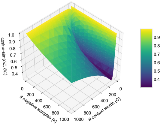
Figure 1: Cosine similarity of incorrect to correct stochastic gradient as a function of $C$ and $k$ assuming that the norm of the gradient with respect to each embedding is fixed to a shared constant. The minimum cosine similarity displayed in this plot is 0.303.

Where $C$ is the number of context tokens and $k$ is the number of negative samples. For a moderate context width, as the number of negative examples increases, the faulty update points further away from the true gradient (Figure 1). See Appendix E for the full derivation.

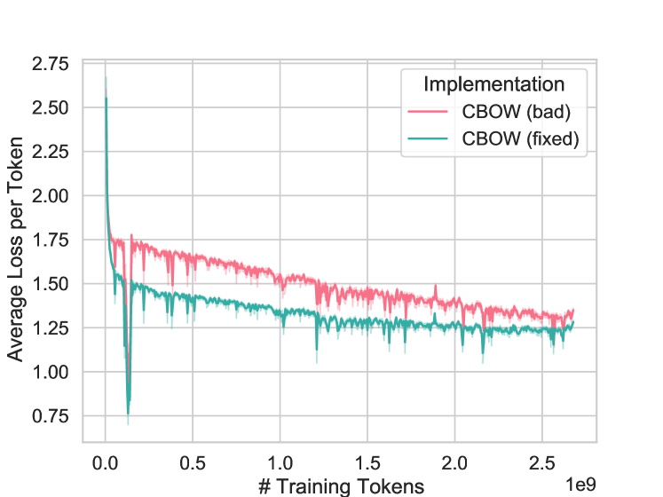
Figure 2: Average negative sampling loss per token for every batch of 5 million tokens for a single epoch of CBOW training on Wikipedia. The shaded region corresponds to the 95% bootstrapped confidence interval over average token loss on 100K token batches.

In practice, we found performance of CBOW embeddings to only decay moderately as a function of number of negatives, regardless of correction to the update, consistent with that reported in Pennington et al. (2014). Nevertheless, we find that our correct CBOW implementation decreases training loss more quickly than the incorrect update, even in the typical setting of 5 negative samples and context width of 5 (Figure 2). Ultimately, increased sensitivity to hyperparameters is not a concern under typical training regimes.

FastText

Although we do not investigate fastText specifically in this work, we do note in Section 2 that fastText CBOW defaults to using the same incorrect source embedding gradient. Sent2vec Gupta et al. (2019) is also exposed to this bug, since it builds on fastText. In spite of this, fastText embeddings trained with the CBOW objective were found to outperform SG across multiple languages Grave et al. (2018). To achieve better performance of CBOW, Grave et al. (2018) tuned hyperparameters and trained on a web-scale corpus (enabled by the faster CBOW training).

FastText also represents each word vector as the sum of vectors of its constituent character n-grams, and includes positional embeddings as part of the training procedure. In this work, we only consider the original CBOW and SG models described in Mikolov et al. (2013a) and hold hyperparameters and training set fixed between models whenever possible. We leave investigation of whether correcting this gradient bug could further improve fastText embeddings as future work.

6 Conclusion

Before the widespread adoption of automatic differentiation libraries, it was the modeler’s responsibility to derive the correct gradient for updating model weights. This word2vec.c gradient bug could have been avoided if a finite difference check was run to ensure the derivation of the stochastic gradient was correct. These checks are standard practice Bengio (2012); Bottou (2012), and we strongly encourage other researchers to use finite difference gradient checks to verify the correctness of manually derived gradients. According to Bottou (2012): “When the computation of the gradients is slightly incorrect, stochastic gradient descent often works slowly and erratically… It is not uncommon to discover such bugs in SGD code that has been quietly used for years.”

We find that CBOW can learn embeddings that are as performant as SG, when trained with the correct update, allowing efficient training of strong word embeddings on web-scale datasets on an academic budget. We release our implementation, kōan, along with trained C4 CBOW embeddings at https://github.com/bloomberg/koan.

Appendix A Versions of Gensim and word2vec.c

We compare against the Gensim implementation at commit

a93067d2ea78916cb587552ba0fd22727c4b40ab

and the word2vec.c implementation at commit

e092540633572b883e25b367938b0cca2cf3c0e7

which are the most recent commits at the time of writing.

Appendix B Training time

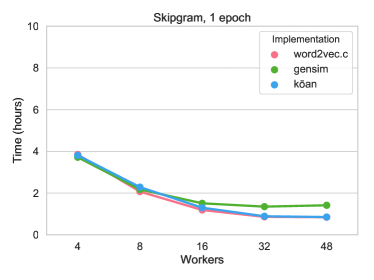
Figure 3: Hours to train CBOW (left) and SG (right) embeddings as a function of number of worker threads for different Word2vec implementations.

Figure 3 shows the time to train each set of embeddings as a function of number of worker threads on the tokenized Wikipedia corpus. All implementations were benchmarked on an Amazon EC2 c5.metal instance (96 logical processors, 196GB memory) using time, and embeddings were trained with a minimum token frequency of 10 and downsampling frequency threshold of $10^{-3}$. We benchmark our implementation with a buffer of 100,000 sentences. We trained CBOW for five epochs and SG for a single epoch, as it is much slower. Gensim seems to have trouble exploiting more worker threads when training CBOW, and both word2vec.c and our implementation learn embeddings faster. word2vec.c achieves slightly better scaling than our implementation during CBOW training (68m46s vs. 72m57s for 48 threads), although ours is faster with fewer workers (e.g., 559m0s vs. 284m58s for 4 threads and 88m28s vs. 72m29s for 32 threads). Although we did not comprehensively benchmark SG training for 5 epochs, we found that training SG embeddings for 5 epochs with 48 threads took us 3.31 times as long as training CBOW.

Appendix C Extrinsic Evaluation Hyperparameters

We evaluate a given set of embeddings on GLUE tasks by using the frozen pre-trained word embeddings in a neural classifier. Words that were out of vocabulary are represented with a zero embedding vector. We use a two layer BiLSTM with 1024 hidden layer width, and a final projection layer. For the NLI tasks, we encode each sequence with an independent BiLSTM encoder. If the embeddings of sequence 1 and 2 are $v$ and $w$, respectively, then a prediction is made using a multilayer perceptron over $[v;w;v-w;v\odot w]$ with a single 512 unit hidden layer. This is identical to the NLI classifier described in Wang et al. (2018). We performed a random search over dropout rate $\in[0.0,0.7]$ and learning rate $\in[10^{-6},10^{-2}]$ with a budget of ten runs. All models are trained for up to 100 epochs with a patience of 2 epochs for early stopping. The same set of sampled hyperparameters was used for model selection for each set of word embeddings.

Appendix D CBOW Embedding Norm

If we train embeddings using the correct implementation of CBOW, the $l_{2}$ norms of target and source vectors are unaffected by the width of the context window (Figure 4). With the faulty implementation Equation 1, the source vector norms increase as a function of the maximum context window width. Growing source norms can be a problem during learning, as larger embedding norms can easily lead to saturated sigmoid activations, effectively halting learning. This problem is further exacerbated by fast implementations of CBOW and SG that approximate the sigmoid activation function by a piecewise linear function. In these approximations, when the logit is above or below some threshold (e.g., 6 and -6 for word2vec.c) and the prediction agrees with ground truth, the gradient for this example is not back-propagated at all.

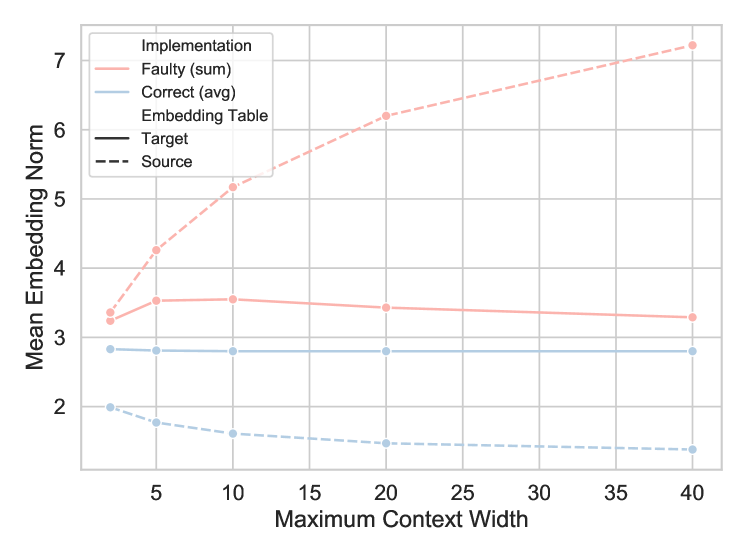
Figure 4: Average target and source vector norms as a function of context width for the correct and incorrect implementations of CBOW. All embeddings were trained for five epochs over a one million sentence sample of the Wikipedia corpus.

Appendix E Analysis of the Incorrect CBOW Gradient

Relationship to correct CBOW update

Although the incorrect CBOW update for source and target embeddings points in a different direction than the SGD update, this is still a descent direction for the CBOW loss. In other words, taking a sufficiently small step in this direction will reduce the stochastic loss. This can be easily seen by:

$$D= \left(\begin{array}[]{c|c}CI_{dC}&0\\ \hline\cr 0&I_{d(k+1)}\end{array}\right)$$ (6)

$$\delta v= [\frac{\partial\mathcal{L}}{\partial v_{w_{1}}};\ldots;\frac{\partial\mathcal{L}}{\partial v_{w_{C}}}]$$

$$\delta v^{\prime}= [\frac{\partial\mathcal{L}}{\partial v^{\prime}_{n_{1}}};\ldots;\frac{\partial\mathcal{L}}{\partial v^{\prime}_{n_{k}}};\frac{\partial\mathcal{L}}{\partial v^{\prime}_{w_{O}}}]$$

$$\delta\theta= [\frac{\partial\mathcal{L}}{\partial v};\frac{\partial\mathcal{L}}{\partial v^{\prime}}]$$

$$\widetilde{\delta\theta}= D\left(\delta\theta\right)$$ (7)

where $d$ is the word embedding dimensionality, $D$ is a diagonal matrix that scales the gradient with respect to each context word by $C$, and leaves the gradient with respect to the negative sampled target words and true target word unchanged. $\delta\theta$ and $\widetilde{\delta\theta}$ denote the correct and incorrect gradients of the loss, respectively, with respect to source and target embeddings. Since all diagonal entries on $D$ are strictly positive, $D$ is positive definite. Therefore, if $\|\delta\theta\|>0$ then $(-\widetilde{\delta\theta})^{T}\delta\theta<0$ and $-\widetilde{\delta\theta}$ is a descent direction for the stochastic loss (Boyd and Vandenberghe, 2004).

Even though the incorrect negative gradient is guaranteed to be a descent direction, the angle between this descent direction and the negative gradient can be influenced by the number of negative samples and the number of context words to average over. For the sake of simplicity, suppose that the gradient of the loss with respect to each source and target embedding has the same norm: $\forall j\in\{1,\ldots,C\},i\in\{1,\ldots,k\}:\|\frac{\partial L}{\partial v_{w_{j}}}\|^{2}_{2}=\|\frac{\partial L}{\partial v^{\prime}_{n_{i}}}\|^{2}_{2}=\alpha$. Then the cosine similarity between the incorrect and correct gradient can be written as:

$$\texttt{cos}(\widetilde{\delta\theta},\delta\theta) =\frac{(\widetilde{\delta\theta})^{T}\delta\theta}{\|\widetilde{\delta\theta}\|_{2}\|\delta\theta\|_{2}}$$

$$=\frac{(C^{2}+k+1)\alpha}{\sqrt{(C^{3}+k+1)\alpha}\sqrt{(C+k+1)\alpha}}$$

$$=\frac{(C^{2}+k+1)}{\sqrt{(C^{3}+k+1)(C+k+1)}}$$

We can better understand how the angle between the incorrect and correct gradient varies as a function of number of context words and negative samples by looking at a plot of this function (Figure 1). What this plot makes clear is that for a moderate number of context words (around 10, which corresponds to a maximum context window of 5), the incorrect stochastic gradient can differ significantly from the true gradient as the number of negative samples increases. However, for sensible settings of $C,k\leq 20$, the minimum cosine similarity is 0.68, achieved by $C=9$ and $k=20$, with 0.82 cosine similarity with $C=5$ and $k=5$ (typical for Word2vec training). Because of this, the CBOW update bug may have gone unnoticed. If one were to sample a large number of negatives, then the bug may have been more apparent.

References

- Bengio (2012) Yoshua Bengio. 2012. Practical recommendations for gradient-based training of deep architectures. In Neural networks: Tricks of the trade, pages 437–478. Springer.
- Bojanowski et al. (2017) Piotr Bojanowski, Edouard Grave, Armand Joulin, and Tomas Mikolov. 2017. Enriching word vectors with subword information. Transactions of the Association for Computational Linguistics, 5:135–146.
- Bottou (2012) Léon Bottou. 2012. Stochastic gradient descent tricks. In Neural networks: Tricks of the trade, pages 421–436. Springer.
- Boyd and Vandenberghe (2004) Stephen P Boyd and Lieven Vandenberghe. 2004. Convex optimization. Cambridge university press.
- Devlin et al. (2019) Jacob Devlin, Ming-Wei Chang, Kenton Lee, and Kristina Toutanova. 2019. Bert: Pre-training of deep bidirectional transformers for language understanding. In Proceedings of the 2019 Conference of the North American Chapter of the Association for Computational Linguistics: Human Language Technologies, Volume 1 (Long and Short Papers), pages 4171–4186.
- Grave et al. (2018) Édouard Grave, Piotr Bojanowski, Prakhar Gupta, Armand Joulin, and Tomáš Mikolov. 2018. Learning word vectors for 157 languages. In Proceedings of the Eleventh International Conference on Language Resources and Evaluation (LREC 2018).
- Gupta et al. (2019) Prakhar Gupta, Matteo Pagliardini, and Martin Jaggi. 2019. Better word embeddings by disentangling contextual n-gram information. In Proceedings of the 2019 Conference of the North American Chapter of the Association for Computational Linguistics: Human Language Technologies, Volume 1 (Long and Short Papers), pages 933–939, Minneapolis, Minnesota. Association for Computational Linguistics.
- Levy and Goldberg (2014) Omer Levy and Yoav Goldberg. 2014. Neural word embedding as implicit matrix factorization. In Advances in neural information processing systems, pages 2177–2185.
- Luong et al. (2013) Minh-Thang Luong, Richard Socher, and Christopher D Manning. 2013. Better word representations with recursive neural networks for morphology. In Proceedings of the Seventeenth Conference on Computational Natural Language Learning, pages 104–113.
- Mikolov (2013) Mikolov. 2013. Google Code Archive: word2vec. https://code.google.com/archive/p/word2vec/.
- Mikolov et al. (2013a) Tomas Mikolov, Kai Chen, Greg Corrado, and Jeffrey Dean. 2013a. Efficient estimation of word representations in vector space. arXiv preprint arXiv:1301.3781.
- Mikolov et al. (2013b) Tomas Mikolov, Ilya Sutskever, Kai Chen, Greg S Corrado, and Jeff Dean. 2013b. Distributed representations of words and phrases and their compositionality. In Advances in neural information processing systems, pages 3111–3119.
- Pennington et al. (2014) Jeffrey Pennington, Richard Socher, and Christopher D Manning. 2014. Glove: Global vectors for word representation. In Proceedings of the 2014 conference on empirical methods in natural language processing (EMNLP), pages 1532–1543.
- Raffel et al. (2020) Colin Raffel, Noam Shazeer, Adam Roberts, Katherine Lee, Sharan Narang, Michael Matena, Yanqi Zhou, Wei Li, and Peter J Liu. 2020. Exploring the limits of transfer learning with a unified text-to-text transformer. Journal of Machine Learning Research, 21:1–67.
- Řehůřek and Sojka (2010) Radim Řehůřek and Petr Sojka. 2010. Software Framework for Topic Modelling with Large Corpora. In Proceedings of the LREC 2010 Workshop on New Challenges for NLP Frameworks, pages 45–50, Valletta, Malta. ELRA. http://is.muni.cz/publication/884893/en.
- Sang and De Meulder (2003) Erik F Sang and Fien De Meulder. 2003. Introduction to the conll-2003 shared task: Language-independent named entity recognition. arXiv preprint cs/0306050.
- Stratos et al. (2015) Karl Stratos, Michael Collins, and Daniel Hsu. 2015. Model-based word embeddings from decompositions of count matrices. In Proceedings of the 53rd Annual Meeting of the Association for Computational Linguistics and the 7th International Joint Conference on Natural Language Processing (Volume 1: Long Papers), pages 1282–1291.
- Wang et al. (2018) Alex Wang, Amanpreet Singh, Julian Michael, Felix Hill, Omer Levy, and Samuel Bowman. 2018. Glue: A multi-task benchmark and analysis platform for natural language understanding. In Proceedings of the 2018 EMNLP Workshop BlackboxNLP: Analyzing and Interpreting Neural Networks for NLP, pages 353–355.