Footprints of impurity quantum phase transitions in quantum Monte Carlo statistics

Abstract

Interacting single-level quantum dot connected to BCS superconducting leads represents a well-controllable system to study the interplay between the correlation effects and the electron pairing that can result in a $0-\pi$ (singlet-doublet) quantum phase transition. The physics of this system can be well described by the impurity Anderson model. We present an analysis of the statistics of the perturbation expansion order of the continuous-time hybridization expansion quantum Monte Carlo algorithm in the vicinity of such a first-order impurity quantum phase transition. By calculating the moments of the histograms of the expansion order which deviate from the ideal Gaussian shape, we provide an insight into the thermodynamic mixing of the two phases at low but finite temperatures which is reflected in the bimodal nature of the histograms.

I Introduction

Advances in the fabrication of nanodevices have enabled us to connect quantum dots with superconducting leads, forming superconducting quantum dot nanostructures. Many experimental realizations utilizing carbon nanotubes, semiconducting nanowires or even single molecules as central active elements demonstrate the large versatility of the concept which attracted a lot of attention (for the overview see Refs. [1, 2, 3]).

In many cases the system can be well described by the single-impurity Anderson model (SIAM) coupled to superconducting BCS leads [4]. This model may exhibit, depending on the parameters, a so-called $0-\pi$ transition signaled by the sign reversal of the supercurrent. This transition is governed by the underlying quantum critical point (QCP) and can be induced by changing the experimentally controllable model parameters such as the local energy level (gate voltage) or superconducting phase difference (magnetic flux in SQUID geometry) as well as by changing parameters that are hard to control in experiment, e.g. the local on-dot Coulomb interaction or the tunneling rate between a lead and a dot.

The usual method of choice for solving the superconducting SIAM is the numerical renormalization group (NRG) method [5]. It works at zero and low temperatures and provides direct access to the one-particle spectral function. The drawback of this method is the inability to solve this model using reasonable computational resources for more than two lead channels, e.g., in a case with an additional metallic lead. Despite the recent progress in this area [6] it still hinders the usability of NRG in multi-terminal and multi-dot setups.

Another class of numerically exact methods to solve SIAM are the quantum Monte Carlo (QMC) techniques. Many flavours of QMC were already employed to solve the superconducting SIAM including the Hirsch-Fye [7] and the continuous-time implementations in either interaction expansion (CT-INT) [8, 4] or hybridization expansion (CT-HYB) [9, 10] formalism. All these algorithms work in the imaginary time domain and are therefore bound to finite temperatures with unpleasant scaling properties with decreasing temperature. Also, obtaining the spectral function requires to perform an analytic continuation to real frequency domain from stochastic imaginary time data which is a notoriously ill-defined problem [11]. Nevertheless, QMC can provide unbiased finite-temperature results and invaluable insight into the thermal effects.

Some of the most interesting effects in superconducting quantum dots are realized in the vicinity of the $0-\pi$ impurity quantum phase transition (QPT). This transition is of the first order and is induced by a crossing of the two lowest-lying many-body eigenstates - a spin-singlet and a spin-doublet [12]. A convenient tool to study a QPT is the so-called fidelity which is a measure of the overlap of ground states of quantum systems sharing the same Hamiltonian but associated with different Hamiltonian parameters [13, 14, 15, 16]. This quantity is by definition very sensitive to the change of the ground state induced by the variation of a control parameter. A method how to extract fidelity and its second derivative w.r.t the change of the control parameter - the fidelity susceptibility, from various QMC methods was used to study QPT in bulk (in Hubbard and Heisenberg models [17, 18]) as well as impurity (in the two-orbital Anderson model [19]) systems. Unfortunately the calculation of the fidelity susceptibility is not implemented by default in most of the publicly available QMC solvers (except the iQIST package [20]).

In this paper we show that a different and valuable insight into the properties of a system close to a QPT can be obtained by studying the statistics of the perturbation expansion order from a CT-HYB calculation. We utilize the CT-HYB method to study the $0-\pi$ transition in superconducting impurity Anderson model (SCIAM). This scenario is rather different from QPT in bulk models (Hubbard or Heisenberg) as we are dealing with an impurity QPT in a zero-dimensional system where the usual concepts like correlation length and finite-size scaling are not defined.

We quantify the unusual non-Gaussian shape of the histograms of the expansion order using the first four moments: mean, variance, skewness and excess kurtosis and discuss their behavior by changing the control parameters and the temperature. We show how the position of the QPT at zero temperatures can be extracted from the average expansion order and how is the thermodynamic mixing of the two phases reflected in the higher moments. Finally, we illustrate the applicability of this method in the Kondo regime by providing results on the BCS-Kondo crossover which leaves a distinct trace on the variance of the expansion order.

The paper is organized as follows. In Sec. II we introduce the SCIAM and the transformation that allows us to use CT-HYB to solve it. Sec. III introduces the moments of the expansion order and explains how they describe the statistics of a random variable. In Sec. IV we present and discuss results on the behavior of the system using the local energy as a control parameter and their connection to previous results from Ref. [21]. We explain the unusual bimodal shape of the histogram of the expansion order and how is it reflected in the moments. We also briefly discuss how the BCS-Kondo crossover in the narrow-gap limit is reflected on the second statistical moment. The main points are then summarized in Sec. V. In Appendix. A we discuss an alternative fit of the histograms far from the QPT. Finally, Appendix. B presents more data obtained by changing other control parameters, namely the interaction strength and the superconducting phase difference, showing the universality of the results from Sec. IV.

II Superconducting impurity Anderson model

II.1 Model formulation

The Hamiltonian of a spinful, single-level quantum dot connected to left (L) and right (R) phase-biased superconducting leads reads

$$\mathcal{H}=\mathcal{H}_{\mathrm{dot}}+\mathcal{H}_{\mathrm{lead}}+\mathcal{H}_{\mathrm{hyb}}$$ (1)

where the quantum dot is described by

$$\mathcal{H}_{\mathrm{dot}}=\sum_{\sigma}\varepsilon_{\sigma}d^{\dagger}_{\sigma}d^{\phantom{{\dagger}}}_{\sigma}+U\left(d^{\dagger}_{\uparrow}d^{\phantom{{\dagger}}}_{\uparrow}-\frac{1}{2}\right)\left(d^{\dagger}_{\downarrow}d^{\phantom{{\dagger}}}_{\downarrow}-\frac{1}{2}\right)$$ (2)

where $d^{\dagger}_{\sigma}$ creates an on-dot electron with spin $\sigma\in\{\uparrow,\downarrow\}$, $\varepsilon_{\sigma}=\varepsilon-\sigma B$ is the local energy level, $B$ is the magnetic field, $U$ is the on-site Coulomb interaction and the local energy is shifted in a way that $\varepsilon=0$ always represents a half-filled dot. The non-interacting electrons in the leads are described by BCS Hamiltonians

$$\mathcal{H}_{\mathrm{lead}} =\sum_{\alpha\mathbf{k}\sigma}\varepsilon^{\phantom{{\dagger}}}_{\alpha\mathbf{k}\sigma}c^{\dagger}_{\alpha\mathbf{k}\sigma}c^{\phantom{{\dagger}}}_{\alpha\mathbf{k}\sigma}$$ (3)

$$-\Delta\sum_{\alpha\mathbf{k}}\left(e^{i\varphi_{\alpha}}c^{\dagger}_{\alpha\mathbf{k}\uparrow}c^{\dagger}_{\alpha\mathbf{\bar{k}}\downarrow}+\mathrm{H.c.}\right)$$

where $c^{\dagger}_{\alpha\mathbf{k}\sigma}$ creates an electron in lead $\alpha\in\{L,R\}$ with spin $\sigma$ and energy $\varepsilon_{\alpha\mathbf{k}\sigma}$, and $\Delta e^{i\varphi_{\alpha}}$ is the complex superconducting order parameter for lead $\alpha$ with amplitude $\Delta$ and phase $\varphi_{\alpha}$. Here we assume that the amplitude is the same in both leads (i.e. they are made from the same material) but the phases can differ. We note that physical observables can only depend on the phase difference $\varphi=\varphi_{L}-\varphi_{R}$ and not on the individual values, i.e. the system must be invariant w.r.t. a global phase shift $\varphi_{\alpha}\rightarrow\varphi_{\alpha}+\varphi_{sh}$ [3]. We also denoted $\mathbf{\bar{k}}=-\mathbf{k}$ to save space in equations. The coupling between the dot and the leads is governed by

$$\mathcal{H}_{\mathrm{hyb}}=-\sum_{\alpha\mathbf{k}\sigma}\left(V^{\phantom{{\dagger}}}_{\alpha\mathbf{k}\sigma}c^{\dagger}_{\alpha\mathbf{k}\sigma}d^{\phantom{{\dagger}}}_{\sigma}+\mathrm{H.c.}\right)$$ (4)

where $V_{\alpha\mathbf{k}\sigma}$ is the tunnel matrix element.

As the Hamiltonian in (1) does not conserve charge, we cannot use the standard CT-HYB algorithm right away to solve it. Therefore we perform a canonical particle-hole transformation in the spin-down segment of the Hilbert space. Following Ref. [8] we define

$$\left(\tilde{c}^{\phantom{{\dagger}}}_{\alpha\mathbf{k}\uparrow},\tilde{c}^{\dagger}_{\alpha\mathbf{k}\uparrow},\tilde{c}^{\phantom{{\dagger}}}_{\alpha\mathbf{k}\downarrow},\tilde{c}^{\dagger}_{\alpha\mathbf{k}\downarrow}\right) =\left(c^{\phantom{{\dagger}}}_{\alpha\mathbf{k}\uparrow},c^{\dagger}_{\alpha\mathbf{k}\uparrow},c^{\dagger}_{\alpha\mathbf{\bar{k}}\downarrow},c^{\phantom{{\dagger}}}_{\alpha\mathbf{\bar{k}}\downarrow}\right),$$ (5)

$$\left(\tilde{d}^{\phantom{{\dagger}}}_{\uparrow},\tilde{d}^{\dagger}_{\uparrow},\tilde{d}^{\phantom{{\dagger}}}_{\downarrow},\tilde{d}^{\dagger}_{\downarrow}\right) =\left(d^{\phantom{{\dagger}}}_{\uparrow},d^{\dagger}_{\uparrow},d^{\dagger}_{\downarrow},d^{\phantom{{\dagger}}}_{\downarrow}\right)$$

which maps the SCIAM (1) on the SIAM with non-superconducting bath but with attractive on-site interaction strength $-U$. We can define Nambu-like spinors in this basis as

$$\tilde{D}=\begin{pmatrix}\tilde{d}_{\uparrow}\\[3.00003pt] \tilde{d}_{\downarrow}\end{pmatrix},\quad\tilde{C}_{\alpha\mathbf{k}}=\begin{pmatrix}\tilde{c}_{\alpha\mathbf{k}\uparrow}\\[3.00003pt] \tilde{c}_{\alpha\mathbf{\bar{k}}\downarrow}\end{pmatrix}.$$ (6)

From now on we drop the spin index in the dispersion $\varepsilon_{\alpha\mathbf{k}}$ and the tunnel coupling element $V_{\alpha\mathbf{k}}$. Let us define matrices

$$E_{\alpha\mathbf{k}}=\begin{pmatrix}\varepsilon_{\alpha\mathbf{k}}&-\Delta e^{i\varphi_{\alpha}}\\[3.00003pt] -\Delta e^{-i\varphi_{\alpha}}&-\varepsilon_{\alpha\mathbf{\bar{k}}}\end{pmatrix},\quad E_{d}=\begin{pmatrix}\varepsilon_{\uparrow}&0\\[3.00003pt] 0&U-\varepsilon_{\downarrow}\end{pmatrix}.$$ (7)

The Hamiltonian in (1) can be rewritten in the form

$$\mathcal{H}_{\mathrm{dot}} =\tilde{D}^{\dagger}E_{d}\tilde{D}-U\left(\tilde{d}^{\dagger}_{\uparrow}\tilde{d}^{\phantom{{\dagger}}}_{\uparrow}-\frac{1}{2}\right)\left(\tilde{d}^{\dagger}_{\downarrow}\tilde{d}^{\phantom{{\dagger}}}_{\downarrow}+\frac{1}{2}\right),$$ (8)

$$\mathcal{H}_{\mathrm{lead}} =\sum_{\alpha\mathbf{k}}\tilde{C}^{\dagger}_{\alpha\mathbf{k}}E_{\alpha\mathbf{k}}\tilde{C}_{\alpha\mathbf{k}},$$

$$\mathcal{H}_{\mathrm{hyb}} =-\sum_{\alpha\mathbf{k}}\left(\tilde{C}^{\dagger}_{\alpha\mathbf{k}}V_{\alpha\mathbf{k}}\sigma_{z}\tilde{D}+\mathrm{H.c.}\right)$$

where $\sigma_{z}$ is a Pauli matrix. The occupation numbers transform as

$$n =n_{\uparrow}+n_{\downarrow}=\tilde{n}_{\uparrow}-\tilde{n}_{\downarrow}+1$$ (9)

$$m =n_{\uparrow}-n_{\downarrow}=\tilde{n}_{\uparrow}+\tilde{n}_{\downarrow}-1$$

$$\nu =\tilde{\nu}$$

where $n_{\sigma}=\langle d^{\dagger}_{\sigma}d^{\phantom{{\dagger}}}_{\sigma}\rangle$ is the spin-resolved electron density, $n$ is the total charge, $m$ is the magnetization and $\nu=\langle d_{\downarrow}d_{\uparrow}\rangle$ is the on-dot induced pairing.

From now on we assume the tunneling density of states (DOS) to be constant in the relevant energy window,

$$A_{T\alpha}(\omega)=\pi\sum_{\mathbf{k}}|V_{\alpha\mathbf{k}}|^{2}\delta(\omega-\varepsilon_{\alpha\mathbf{k}})=\Gamma_{\alpha}\Theta(W^{2}-\omega^{2})$$ (10)

where $W$ is the half-bandwidth of the non-interacting band. As the relevant energy scale for this model is the superconducting gap $\Delta$ which is usually of order of $100~{}\mu$eV, the assumption of constant DOS over such a narrow energy window is justifiable in most experimentally relevant situations. Equation (10) also defines the tunneling rates $\Gamma_{\alpha}$ which, for $\mathbf{k}$-independent tunnel matrix elements $V$ can be expressed as $\Gamma_{\alpha}=\pi|V_{\alpha}|^{2}/(2W)$. We will focus only on the situations with symmetric coupling $\Gamma_{L}=\Gamma_{R}=\Gamma/2$ as any asymmetric setup with $\Gamma_{L}\neq\Gamma_{R}$ can be mapped on the symmetric one using a simple formula [22].

The total effect of a lead $\alpha$ on the impurity can be summed into a hybridization function which describes the hopping from the impurity to the lead $\alpha$, the propagation through the lead and the hopping back to the impurity. It can be represented in the imaginary-frequency (Matsubara) domain as

$$\Gamma_{\alpha}(i\omega_{n})=\sum_{\mathbf{k}}V_{\alpha\mathbf{k}}^{*}\sigma_{z}[i\omega_{n}I_{2}-E_{\alpha\mathbf{k}}]^{-1}\sigma_{z}V_{\alpha\mathbf{k}}$$ (11)

where $I_{2}$ is the $2\times 2$ unit matrix, $\omega_{n}=(2n+1)\pi/\beta$ is the $n$th Matsubara frequency and $\beta=1/(k_{B}T)$ is the inverse temperature. Under the assumption of a constant tunneling DOS (10), the hybridization function of the lead $\alpha\in\{L,R\}$ can be expressed as

$$\Gamma_{\alpha}(i\omega_{n})=-\frac{\Gamma_{\alpha}w(i\omega_{n})}{\sqrt{\omega_{n}^{2}+\Delta^{2}}}\begin{pmatrix}i\omega_{n}&\Delta e^{i\phi_{\alpha}}\\[3.00003pt] \Delta e^{-i\phi_{\alpha}}&i\omega_{n}\end{pmatrix}$$ (12)

where $w(i\omega_{n})=(2/\pi)\arctan(W/\sqrt{\omega_{n}^{2}+\Delta^{2}})$ is the correction due to finite bandwidth that approaches unity for $W\rightarrow\infty$.

II.2 $0-\pi$ quantum phase transition

The so-called $0-\pi$ QPT corresponds to the change of the ground state from a non-magnetic singlet ($0$ phase) to a spin-degenerate doublet ($\pi$ phase). It is signaled at zero temperatures by the abrupt change of the sign of both the Josephson current and the on-dot induced pairing from positive in $0$-phase to negative in $\pi$ phase [23, 24, 25], and the crossing of the subgap, Andreev bound states at the Fermi energy [26, 27, 28]. As this transition is of the first order, the finite-temperature state is a simple thermodynamic mixture of the two phases and the transition is smeared out by increasing temperature into a crossover.

The method of extraction of the position of the QPT at zero temperature from finite temperature (experimental or QMC) data was already discussed in Ref. [21]. For low temperatures, only the lowest-lying many-body states are significant. Due to the presence of a superconducting pairing, these states are discrete and separated from the continuous part by a gap of the order of $\Delta$. In the absence of magnetic field, we are dealing with a one spin singlet and one spin doublet. The second discrete singlet state and the continuum of states lie higher in energy and can be neglected at low temperatures. The canonical average of an observable $F$ then reads

$$\langle F(x)\rangle =\frac{1}{\mathcal{Z}}\sum_{n}F_{n}(x)e^{-\beta E_{n}(x)}$$ (13)

$$\approx\frac{F_{s}(x)e^{-\beta E_{s}(x)}+2F_{d}(x)e^{-\beta E_{d}(x)}}{e^{-\beta E_{s}(x)}+2e^{-\beta E_{d}(x)}}$$

where $\mathcal{Z}$ is the partition function, $F_{s}$ ($F_{d}$) are zero-temperature values of $F$ in singlet (doublet) state and $x$ is a control parameter (e.g. local energy $\varepsilon$), changing of which crosses the QPT at critical value $x_{c}$. At QPT, the two discrete many-body states cross, i.e., $E_{s}(x_{c})=E_{d}(x_{c})$ and the average of an observable $F$ reads

$$\langle F(x_{c})\rangle=\frac{1}{3}\left[F_{s}(x_{c})+2F_{d}(x_{c})\right].$$ (14)

This value is independent of temperature, which implies that all curves $F(x)$ for low enough temperatures cross at one point and this point marks the position of the QPT at zero temperatures.

III Moments of the expansion order

A complete overview of the CT-HYB method can be found in Ref [29]. It is based on an expansion of the partition function in powers of the hybridization term $\mathcal{H}_{\mathrm{hyb}}$ (4) around $\mathcal{H}_{\mathrm{dot}}+\mathcal{H}_{\mathrm{lead}}$. The order of the expansion $k$ (the number of hybridization events in the given random configuration) depends rather strongly on the model parameters. It scales linearly with inverse temperature $\beta$ and in general decreases with increasing interaction strength $U$. The statistics of $k$ can be accumulated during the Monte Carlo run and represented in the form of a histogram $H(k)$. The moments of $k$ can be then calculated and their analysis provides a deeper insight into the performance of the solver and also the properties of the solved model.

We focus on four moments of the expansion order: mean, variance, skewness and excess kurtosis. The behavior of the variance and the excess kurtosis of $k$ around a phase transition point has been briefly discussed by Huang et al. in an appendix of Ref. [18] for the case of the Mott transition in the single-band Hubbard model within the dynamical mean-field theory (DMFT). As the $0-\pi$ impurity QPT in the superconducting Anderson model is a way simpler scenario than a Mott transition in the Hubbard model, it provides an opportunity to examine their behavior in a well-controllable setup and shed more light on the statistics of the expansion order.

The $n$th central moment of a discrete random variable $k\in\{0,1,2\ldots\}$ is defined as

$$\mu_{n}\equiv\langle(k-c_{n})^{n}\rangle=\frac{1}{N}\sum_{k=0}^{\infty}(k-c_{n})^{n}p(k)$$ (15)

where $p(k)$ is the number of occurrences of given $k$ in the sample, $c_{n}$ is the $n$th central value and $N$ is the number of measurements. The mean $\mu=\mu_{1}$ is the first moment about zero ($c_{1}=0$), and variance as the second moment about the mean ($c_{2}=\mu$),

$$\sigma^{2}=\langle(k-\mu)^{2}\rangle=\langle k^{2}\rangle-\mu^{2}.$$ (16)

For higher moments it is useful to define standardized moments (normalized moments about the mean) $\bar{\mu}_{n}=\mu_{n}/\sigma^{n}$. Skewness and kurtosis are then defined as the third and fourth standardized moments, $\gamma=\bar{\mu}_{3}$ and $\kappa_{0}=\bar{\mu}_{4}$, respectively. As the kurtosis of the Gaussian distribution equals three, it is often convenient to define the excess kurtosis $\kappa=\kappa_{0}-3$. To summarize,

$$\mu =\langle k\rangle,\qquad\qquad\quad\sigma^{2}=\langle(k-\mu)^{2}\rangle,$$ (17)

$$\gamma =\frac{\langle(k-\mu)^{3}\rangle}{\sigma^{3}},\qquad\kappa=\frac{\langle(k-\mu)^{4}\rangle}{\sigma^{4}}-3.$$

The first two moments are standard tools in mathematical statistics and their meaning is clear, but skewness and kurtosis are more abstract quantities. Therefore we illustrate them in Fig. 1. Skewness measures the asymmetry of the tails of a distribution. In panel (a) we plotted distributions with skewness $\gamma>0$ (left-leaning, right tail is longer), $\gamma=0$ (no skew) and $\gamma<0$ (right-leaning, left tail is longer). The excess kurtosis measures how fast the distribution vanishes at higher values compared to the Gaussian. Distributions with $\kappa>0$ (with “fat tails”) are usually referred to as leptokurtic, with $\kappa=0$ as mesokurtic and with $\kappa<0$ (“thin tails”) as platykurtic. Examples of such distributions are plotted in panel (b).

It is worth noting that an alternative way to describe a distribution, complementary to the moments, is with statistical cumulants. The first four cumulants $K_{n}$ of a random variable $k$ are connected to the standardized moments as defined in Eq. (17) as $K_{1}=\mu$, $K_{2}=\sigma^{2}$, $K_{3}=\gamma\sigma^{3}$, and $K_{4}=\kappa\sigma^{4}$, and the cumulant analysis would be analogous to the moment analysis presented below.

The averaged expansion order $\mu$ from CT-HYB also has a physical meaning. In the case of the impurity Anderson model it is connected to the hybridization energy as $\langle k\rangle=\beta E_{\mathrm{hyb}}$ where [30]

$$E_{\mathrm{hyb}}=\langle\mathcal{H}_{\mathrm{hyb}}\rangle\equiv\frac{1}{\mathcal{Z}}\mathop{\rm Tr}\nolimits\left[e^{-\beta\mathcal{H}}\mathcal{H}_{\mathrm{hyb}}\right].$$ (18)

This is one of the differences between a calculation of the impurity Anderson model and a DMFT calculation of the Hubbard model, for which the averaged expansion order from CT-HYB can be identified with the kinetic energy. Here, $E_{\mathrm{hyb}}$ can also be expressed in terms of the local interacting Green function $G(i\omega_{n})=[i\omega_{n}I_{2}-E_{d}-\Sigma(i\omega_{n})]^{-1}$ and the hybridization function $\Gamma(i\omega_{n})$. Here $\Sigma(i\omega_{n})$ is the dynamical self-energy induced by $U$. From the equation of motion we obtain [31]

$$E_{\mathrm{hyb}}=-\frac{1}{\beta}\mathop{\rm Tr}\nolimits\sum_{n}\Gamma(i\omega_{n})G(i\omega_{n}).$$ (19)

This formula can be evaluated numerically and used as a benchmark of the accuracy of the measurement of the local Green function w.r.t. the averaged expansion order.

Figure 1: Examples of distribution functions $p(x)$ with different skewness $\gamma$ (panel a) and excess kurtosis $\kappa$ (panel b).

IV Results

All CT-HYB calculations were performed using the TRIQS/CTHYB 2.2 solver [32]. We set $B=0$, $W=100\Delta$ and the cutoff in Matsubara frequencies $\omega_{n}^{\mathrm{max}}\geq 300\Delta$. We encountered no fermionic sign problem during the calculations. The total charge $n$ and the induced pairing $\nu$ were evaluated by tracing the measured impurity density matrix and using Eq. (9).

IV.1 Shape of histograms around the QPT

In Fig. 2 we plotted the on-dot induced pairing $\nu$ as a function of the local energy $\varepsilon$ for $U=8\Delta$, $\Gamma=\Delta$ and $\varphi=0$ for three values of inverse temperature $\beta\Delta=40$, $20$ and $10$. Here $\varepsilon=0$ represents the half-filled dot. This plot illustrates the typical behavior of SCIAM around the QPT. The induced paring is positive in the $0$-phase and negative in the $\pi$-phase and all lines cross at $\varepsilon_{c}\approx 2.67\Delta$. The position of such a crossing is consistent with the position of the QPT at zero-temperature as explained in Ref. [21]. The inset shows the total on-dot electron density $n$ that decreases as we move away from the half-filled case. Again, all lines cross at the same value of $\varepsilon$, proving the applicability of the formula in (14).

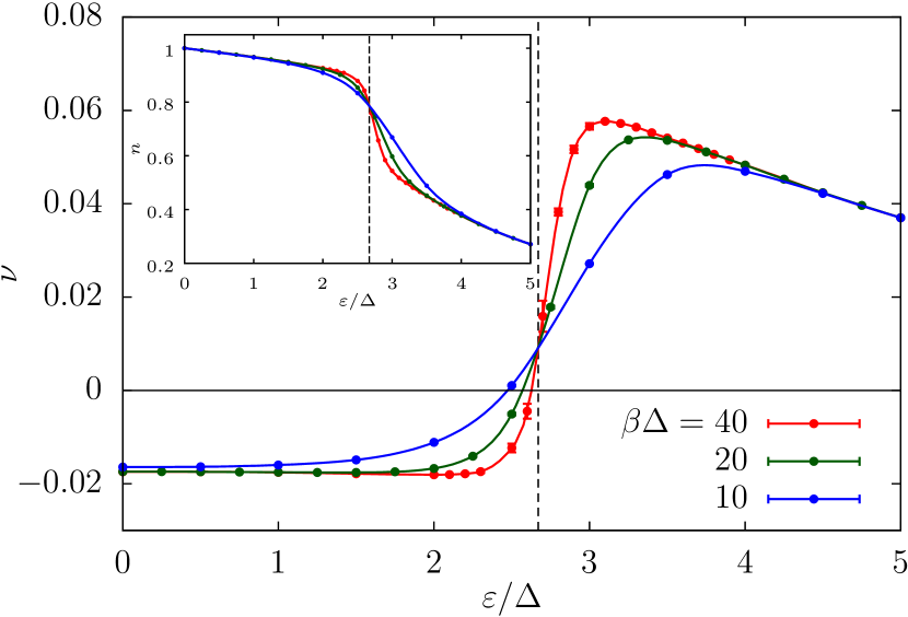
Figure 2: On-dot induced pairing $\nu$ as a function of the local energy $\varepsilon$ calculated using CT-HYB for $U=8\Delta$, $\Gamma=\Delta$ and $\varphi=0$ for three values of inverse temperature $\beta\Delta=40$, $20$ and $10$. Lines are splines of QMC data and serve only as a guide for the eye. All curves cross at $\varepsilon_{c}\approx 2.67\Delta$ within the error bars. Inset: On-dot electron density $n$ for the same set of parameters, showing the same crossing behavior around the critical point as the induced pairing.

The histograms of the expansion order $k$ normalized to the number of QMC measurements ($4.8\times 10^{8}$ in this case) for $\beta\Delta=40$ are plotted in Fig. 3(a) We plotted few histograms around the critical value $\varepsilon_{c}$ (solid lines) together with histograms for values further from the transition point, $\varepsilon=\Delta$ and $\varepsilon=4\Delta$ (dashed lines) for comparison. As the averaged expansion order is rather large, the histograms resemble more a continuous curve than a discrete set of values. It is also the reason why the histograms are not distorted much by the fact that the expansion order is bounded from below by zero. As the averaged expansion order increases with decreasing temperature, it is always possible to run the simulation at low enough temperatures to minimize the distortion.

We see that histograms for $\varepsilon=\Delta$ and $4\Delta$ are of the Gaussian shape. This shape does not change until we approach the critical point. As we move closer, the histogram starts to deviate strongly from a Gaussian, first developing a shoulder and later turning into a broad two-peaked structure. Similar double-peaked histograms were also reported in Ref. [18] for the Hubbard model in the vicinity of the Mott transition. The histograms for values of $\varepsilon$ close to the critical value also intersect at one point at $k\approx 99$. As the two-peak structure can be well fitted by a pair of Gaussians, we can assume these histograms can be also seen as thermal averages over the singlet and doublet ground states,

$$H(k,\varepsilon)\approx\frac{H_{s}(k,\varepsilon)e^{-\beta E_{s}(\varepsilon)}+2H_{d}(k,\varepsilon)e^{-\beta E_{d}(\varepsilon)}}{e^{-\beta E_{s}(\varepsilon)}+2e^{-\beta E_{d}(\varepsilon)}}.$$ (20)

We denote the intersection point of the two histograms as $k_{0}$, so $H_{s}(k_{0},\varepsilon_{c})=H_{d}(k_{0},\varepsilon_{c})$ where we replaced the local energy by its critical value, assuming that the constituent histograms $H_{s}$ and $H_{d}$ do not depend much on $\varepsilon$ around the critical point. As $E_{d}(\varepsilon_{c})=E_{s}(\varepsilon_{c})$, we obtain in the vicinity of the critical point ($\varepsilon\approx\varepsilon_{c}$),

$$H(k_{0},\varepsilon)=H_{s}(k_{0},\varepsilon)=H_{d}(k_{0},\varepsilon)$$ (21)

for all values of $\varepsilon$ close enough to the critical point that we can replace $H_{s,d}(k,\varepsilon)\approx H_{s,d}(k,\varepsilon_{c})$. This feature represents itself as the histograms crossing at the same point at $k=k_{0}$ for $\varepsilon\approx\varepsilon_{c}$. In panels (b)-(e) we plotted selected histograms in the vicinity of the critical point fitted by a pair of Gaussians. This illustrates the feature that the constituent histograms $H_{s}$ and $H_{d}$ do not depend much on $\varepsilon$, only their weights are changing as we cross the transition point.

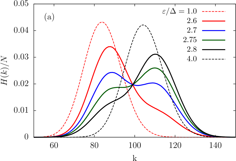
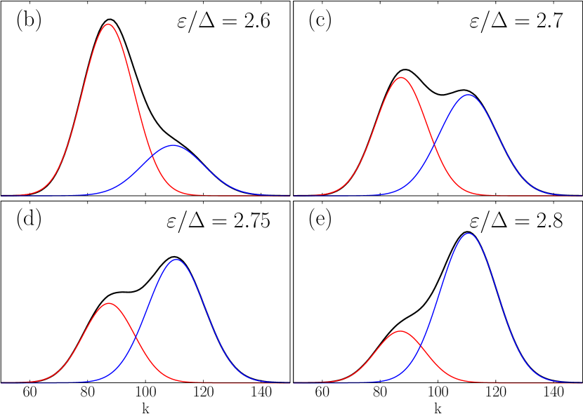
Figure 3: Panel (a): Histograms of the expansion order $k$ from CT-HYB calculation for different values of phase difference around the zero-temperature critical value $\varepsilon_{c}\approx 2.67\Delta$ for the same parameters as in Fig. 2, $U=8\Delta$, $\Gamma=\Delta$ and $\varphi=0$ and inverse temperature $\beta\Delta=40$. All histograms for $\varepsilon$ close to $\varepsilon_{c}$ (solid lines) show a non-Gaussian, two-peak structure and intersect in one point for $k\approx 99$. We added the Gaussian-like histograms for the two values far from the transition point, $\varepsilon=\Delta$ and $\varepsilon=4\Delta$ (dashed lines) for comparison. Panels (b)-(e): Histograms from panel (a) fitted with a pair of Gaussians. Red (blue): contribution from the doublet (singlet) ground state.

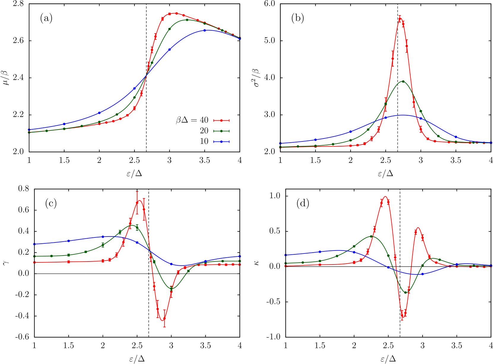
Figure 4: Mean (panel a), variance (b), skewness (c) and excess kurtosis (d) of the expansion order $k$ calculated from the histograms provided by the CT-HYB solver as functions of the local energy $\varepsilon$ for the same parameters as in Fig. 2, $U=8\Delta$, $\Gamma=\Delta$ and $\varphi=0$. Lines are splines of QMC data and serve only as a guide for the eye.

The first four standardized moments (mean, variance, skewness and excess kurtosis) as defined by Eq. (17) calculated from the histograms for the same parameters as in Figs. 2,3 are plotted in Fig. 4. These quantities were calculated using Eq. (15) where we approximated $p(k)$ by the histogram $H(k)$. Panel (a) shows the behavior of the average expansion order $\mu$ scaled to inverse temperature $\beta$ for three values $\beta\Delta=40$, $20$ and $10$. All curves cross at $\varepsilon_{c}$, like the curves for the induced pairing. This is not a surprise since we identified the physical meaning of $\mu/\beta$ as the hybridization energy and at low temperatures Eq. (18) also reduces to a relation in a form of Eq. (14). It proves that the position of the QCP is encoded already in the statistics of the expansion order and can be obtained without actually measuring any physical observable or the one-particle Green function.

We can obtain the same result that lines $\mu(\varepsilon)/\beta$ for different low enough temperatures cross at the same point using the assumption that the histogram in the vicinity of the critical point can be decomposed into parts from the singlet and from the doublet, $H(k,\varepsilon\approx\varepsilon_{c})=[H_{s}(k,\varepsilon)+2H_{d}(k,\varepsilon)]/3$. Then Eq. (15) for $n=1$ and $c_{1}=0$ reduces to a weighted sum of two contributions, $\mu\equiv\langle k\rangle=(\langle k\rangle_{s}+2\langle k\rangle_{d})/3$ where $\langle k\rangle_{s,d}$ is an average of $k$ w.r.t. $H_{s,d}$.

The broadening of the histogram can be quantified by the scaled variance $\sigma^{2}/\beta$ plotted in Fig. 4(b) that shows a peak above $\varepsilon_{c}$. For $\beta\Delta=40$ the peak lies at $\varepsilon\approx 2.72\Delta$ (between the blue and green curves in Fig. 3(a)). The curves for different temperatures do not cross at the same point. Using the same reasoning as for the averaged expansion order we obtain

$$\sigma^{2} \approx\frac{1}{3}\Big{[}\langle k^{2}\rangle_{s}+2\langle k^{2}\rangle_{d}-\frac{1}{9}\left(\langle k\rangle_{s}+2\langle k\rangle_{d}\right)^{2}\Big{]}$$ (22)

$$=\frac{1}{3}(\sigma_{s}^{2}+2\sigma_{d}^{2})+\frac{2}{9}(\langle k\rangle_{s}-\langle k\rangle_{d})^{2}.$$

The first term scales as $\beta$ with temperature while the second scales as $\beta^{2}$. As a result, curves of scaled variance $\sigma^{2}/\beta$ at the transition point do not cross as there is a linear offset due to the last term in Eq. (22). As the width of the crossover region between the two phases is increasing with increasing temperature, the peak in variance becomes wider and less pronounced and the maximum moves away from $\varepsilon_{c}$. As this maximum lies away from the transition point at any finite temperature, variance is not a good estimator of the position of the QPT.

We would like to point out that the fact that the scaled average expansion order $\mu/\beta$ can be identified with the hybridization energy $E_{\mathrm{hyb}}$ does not automatically imply that the variance of the expansion order is identical to the variance of $E_{\mathrm{hyb}}$. The question whether the variance has a physical meaning is beyond the scope of this paper.

The overall shape of the histogram can be well quantified by the skewness $\gamma$ which is plotted in Fig. 4(c). Histograms for low temperatures almost always have a slight positive skewness (leaning to the left). As we approach the QPT by moving away from half-filling (from the $\pi$-phase to the $0$-phase), skewness shows a prominent positive peak connected with the development of the shoulder on the histogram indicating increasing presence of the $0$-phase in the thermal mixture. The skewness is zero at the same point where variance has a maximum, above the zero-temperature QPT. This is the point where the histogram is symmetric due to equal admixtures of the zero and the $\pi$ phases at given temperature. As we move across this point, the scenario is reversed with a negative skewness indicating decreasing presence of the $\pi$ phase. All the features are quickly smeared out by increasing temperature and for $\beta\Delta=10$ the skewness is positive for all values of $\varepsilon$.

The overall positive skewness of the histograms for all temperatures indicates a systematic deviation from the ideal Gaussian shape even far away from the transition point. An alternative fitting of the histograms with a single-parametric Poisson curve that would explain this behavior is discussed in Appendix A.

The curves for different temperatures seem to cross at one point very close to $\varepsilon_{c}$ within the QMC error bars. As skewness in our definition is normalized to $\sigma^{3}$, an analysis analogous to the case of the variance in (22) becomes very tedious and effectively not feasible.However, simple analytical models of appropriate Boltzmann mixtures of two Gaussian or Poisson distributions exhibit qualitatively identical behavior with an apparent common crossing very close to the QPT. Detailed analysis reveals that it is not an exact single crossing, but just series of nearby ones, whose overall position depends on a subtle interplay of cumulants of constituent distributions with the Boltzmann factors. As such, this phenomenon appears to have a rather generic origin and does not reveal any new information about the microscopic features of the underlying model.

The excess kurtosis $\kappa$ provides additional insight into the deviations from a Gaussian shape. It is, in contrast to the skewness, insensitive to which tail of the distribution deviates from the Gaussian, therefore the curve is rather symmetric around $\varepsilon_{c}$. Excess kurtosis is almost zero at low temperatures and far from the transition point indicating that the tails of the histogram are of Gaussian shape. As we move closer to QPT from any side, the histogram becomes leptokurtic (fat-tailed), again because of the presence of the shoulder, as evident from Figs. 3(b),(e). This indicates that configurations with a large or small number of hybridization events are encountered here more often during the QMC sampling. Then it shows a well developed minimum at the same point where skewness crosses zero, i.e. where the histogram is symmetric.

In summary, the abovementioned statistical moments quantify well the shape of the histogram of the expansion order. It changes its shape from nearly ideal Gaussian to bimodal which can be fitted by a pair of Gaussians as a result of the thermodynamic mixing of the two phases at low but finite temperatures. The position of the zero-temperature QCP can be extracted from the crossing of the curves of the first moment for two low-enough temperatures. The extremal points of higher moments (maximum of $\sigma^{2}$, zero of $\gamma$, minimum of $\kappa$) always lie away from the transition point in the direction of the $0$-phase and approach it only slowly with decreasing temperature, therefore they are not good estimators of the position of the QCP, although they provide a way to quantify the mixing of the phases in the crossover region.

IV.2 BCS-Kondo crossover

The moments analysis presented above is largely based on the two-level approximation from Ref. [21] which requires the temperature to be much less than the superconducting gap $\Delta$ so that the continuous parts of the spectra can be neglected in the close vicinity of the QPT. This hinders the effectiveness of this method in the strong-coupling Kondo regime where a narrow gap is required, otherwise the complete Kondo screening is impossible due to the lack of the spectral weight around the Fermi energy [3].

To study the limits of the usefulness of our method in the Kondo regime, we calculated the behavior of the induced gap and the first two moments of the expansion order at half-filling in a narrow-gap limit $\Delta/\Gamma=0.04$ for $\varphi=0$. The results are plotted in Fig. 5.

The inset of panel (a) shows the zero-temperature phase diagram in the $U-\Delta$ plane calculated using NRG taken from Ref. [33]. The nature of the ground state in the singlet phase is governed by the competition between the superconductivity and the Kondo effect and this phase can be in general separated into a region of large gap and small interaction strength where the ground state is ’BCS-like’ and the ’Kondo-like’ region of small gap size and large interaction strength. These two regions are separated by a broad crossover region which is hard to locate as it leaves no trace on the quantities like the electron filling or the induced gap and can be identified usually only from the change of the shape of the spectral function [34].

Panel (a) shows the induced pairing $\nu$ calculated along the blue dashed line in the inset for three inverse temperatures $\beta\Gamma=20$, $40$ and $80$ compared with the zero-temperature NRG result. The $0-\pi$ QPT lies at $U_{c}\approx 12.02\Gamma$. The curves for the two lowest temperatures cross at the transition point while the curve for $\beta\Gamma=20$ is slightly off as this temperature is too high for the applicability of the two-level approximation. The other feature, the crossover between the two types of singlet ground state that takes place at $U\sim 6-8\Gamma$, leaves no trace on the induced pairing.

The scaled variance $\sigma^{2}/\beta$ plotted in panel (b) shows no peak around $U_{c}$ that we could connect with the $0-\pi$ QPT. As the superconducting gap $\Delta$ in this plot is 20-times smaller than in Figs. 2-4, we would need to perform the simulation at inverse temperatures $\beta\Gamma>400$ to obtain similar resolution around the $0-\pi$ QPT as before, which is impossible with the current imaginary-time implementations of the CT-HYB algorithm. On the other hand, the variance for $\beta\Gamma=10$, $20$ and $40$ shows a broad peak in the region where the BCS-Kondo crossover is expected. This peak moves slowly to higher interaction strengths with decreasing temperature. The result for $\beta\Gamma=80$ shows a different profile with flatter top and a more significant shift to higher values of interaction strengths for $U>9\Gamma$. This can be caused by the additional effect of the QCP at $U_{c}$ that starts to have effect on the statistics as we move closer to it by decreasing the temperature.

We thus believe that the variance of the expansion order represents a limited but simple tool to identify a presence of the BCS-Kondo crossover and provides a rough estimate of its position. While we cannot completely rule out the possibility that the peak in the variance is caused solely by the presence of the QCP at $U_{c}$ and is not connected whatsoever to the BCS-Kondo crossover, the different shape of the variance curve for $\beta\Gamma=80$ suggests there are two different phenomena having effect on the statistics. We would need data for much lower temperatures to resolve this issue which hinders the applicability of the presented method in the narrow-gap regime.

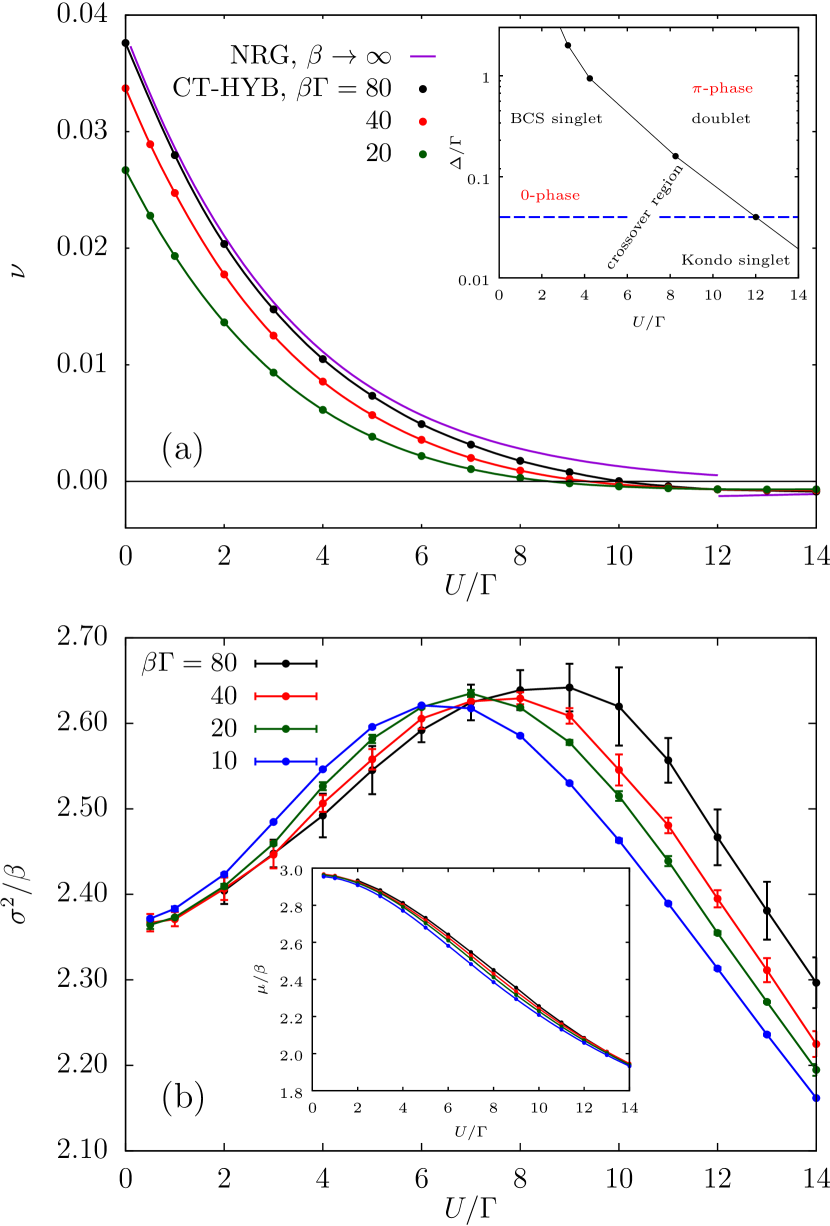
Figure 5: Panel (a): Induced pairing $\nu$ as a function of interaction strength $U/\Gamma$ in the narrow-gap limit $\Delta/\Gamma=0.04$, $\varphi=0$ and $\varepsilon=0$ (half-filling) calculated using CT-HYB for three temperatures and compared with the zero-temperature NRG data taken from Ref. [33]. QMC error bars are smaller than the symbol size. Inset: Phase diagram in the $U-\Delta$ plane. Black bullets are the $0-\pi$ phase boundary at zero temperature calculated using NRG. Blue dashed line marks the cut along which the data in the main plot are calculated. Note the logarithmic scale on the vertical axis. Panel (b): scaled variance $\sigma^{2}/\beta$ of the perturbation order $k$ for the same parameters as the induced gap in panel (a) that shows a broad peak in the crossover region between the BCS-like and the Kondo-like singlet regions. Inset: Scaled mean $\mu/\beta$ for the same parameters as in the main plot. Lines connecting the QMC data points serve only as guides for the eye.

V Conclusions

Superconducting quantum dots provide a simple testbed for studying impurity QPT and this physics can be captured very well by the SCIAM. Numerically exact CT-HYB QMC simulation can provide an unbiased insight into finite-temperature behavior in the vicinity of the critical point. The change of the ground state from non-magnetic singlet to spin-degenerate doublet leaves a unique footprint on the statistics of the hybridization expansion order which is accumulated during the simulation and can be quantified by the moments of its histogram.

The position of the zero-temperature QCP can be extracted from finite-temperature results by measuring two sets of data for any physical observable at two different low-enough temperatures as already discussed in Ref. [21]. As the average expansion order in CT-HYB can be identified with the hybridization energy, it is also a physical observable and therefore position of the QCP can be extracted from its statistics without performing any QMC measurement at all (except a trivial measurement of the average sign). In the vicinity of the critical point the histogram of the expansion order deviates from the ideal Gaussian shape and this deviation can be quantified by the higher moments (variance, skewness, excess kurtosis). We show that the histogram can be separated into Gaussian contributions from the two ground states. The weights of these contributions equalize at the point that linearly approaches the QCP with decreasing temperature and can be identified from the maximum of variance, zero of the skewness or the minimum of the excess kurtosis. While this method is due to limitations on the lowest achievable temperature practically applicable only in situations with relatively large superconducting gap, limited information about the nature of the ground state can be extracted also in the narrow-gap limit.

We believe this analysis can provide additional insight into the physics around an impurity QPT beyond the scope of standard tools like the fidelity susceptibility for systems that can be mapped onto an impurity Anderson model. Furthermore, this analysis can be performed using any available CT-HYB solver without any modification or implementation of new features. The results also hold for any system exhibiting a first-order impurity QPT as well as bulk systems that are treated using the DMFT technique of mapping a lattice model on an effective impurity problem.

Appendix A Alternative fit of the histograms

The overall positive skewness of the histograms even far from the transition point suggests their inherent non-Gaussian nature. To look deeper into this feature we replotted in Fig. 6a two histograms from Fig. 3a for parameters far from the QPT, $\varepsilon=\Delta$ ($\pi$-phase, red) and $\varepsilon=4\Delta$ ($0$-phase, black), on a logarithmic scale together with the Gaussian fit $p(k;\mu,\sigma^{2})=\exp[-(k-\mu)^{2}/(2\sigma^{2})]/\sqrt{2\pi\sigma^{2}}$ (dashed lines). The deviations from the Gaussian shape in both cases are evident.

Considering that the expansion order $k$ is a discrete variable bound from below by zero and assuming that the QMC configurations with a given expansion order are generated as independent rare events, we tried an alternative fitting with the Poisson distribution $\bar{p}(k;\lambda)=\lambda^{k}e^{-\lambda}/k!$ (dash-dotted lines). A distinct feature of the Poisson distribution compared with the Gaussian is that its mean equals the variance, $\mu=\sigma^{2}=\lambda$ so the fitting is single-parametric. As the limit of $\bar{p}(k;\lambda)$ for large $\lambda$ is Gaussian, it is problematic to distinguish the two cases for large mean values and the main clue is the inherent single-parametric nature of $\bar{p}(k;\lambda)$ compared with the two-parametric function $p(k;\mu,\sigma^{2})$.

We see that the histogram for $\varepsilon=\Delta$ ($\pi$-phase) can be very well fitted with a Poisson curve, meanwhile the histogram for $\varepsilon=4\Delta$ ($0$-phase) cannot. To identify the region of validity of this alternative fit we utilize the above mentioned feature of the Poison distribution that $\mu=\sigma^{2}$ and we plotted in Fig. 6b data from Figs. 4a and 4b for $\beta\Delta=40$ into a single plot. The two quantities almost coincide for $0<\varepsilon\lesssim 2\Delta$, that is in the $\pi$-phase (doublet ground state). The values in the $0$-phase are different which confirms the failure of the alternative fit for $\varepsilon=4\Delta$ (black dash-dotted line in Fig. 6a). Resolving the issue why the statistics of the expansion order follows a Poisson distribution in only one of the phases would require a detailed analysis of the configurations encountered during the simulation and also an independent check by a different CT-HYB solver to rule out the effect of the given implementation of the algorithm, which is beyond the scope of this paper.

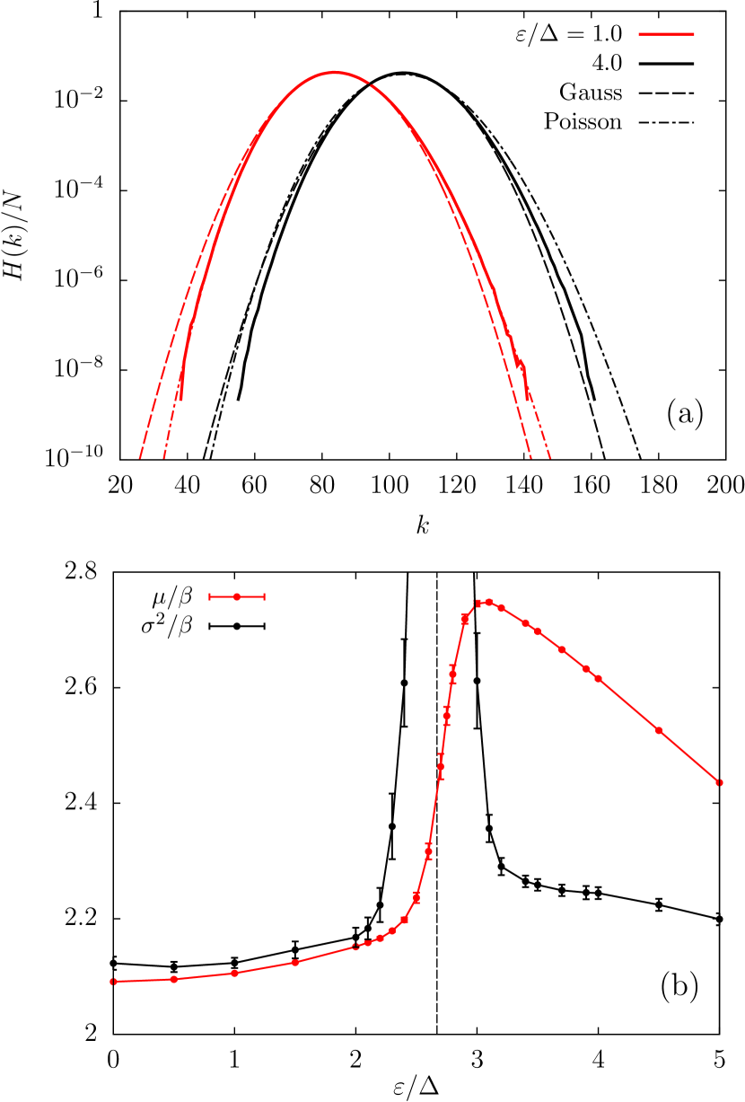
Figure 6: Panel (a): Histograms far from the QPT from Fig. 3a for $\beta\Delta=40$ and parameters $\varepsilon=\Delta$ ($\pi$-phase, red) and $\varepsilon=4\Delta$ ($0$-phase, black) on logarithmic scale fitted by a two-parametric Gaussian function (dashed lines) and by a single-parametric Poisson function (dash-dotted lines). Panel (b): Mean $\mu/\beta$ (red bullets) and variance $\sigma^{2}/\beta$ (black bullets) for $\beta\Delta=40$ from Figs. 4a and 4b plotted in the same figure. Lines are just a guide to the eye. Values of the mean and the variance in the $\pi$-phase ($\varepsilon\lesssim 2\Delta$) almost coincide, showing the region of validity of the single-parametric Poisson fit.

Appendix B Dependence on the interaction strength and phase difference

A superconducting quantum dot can be driven through a QPT by changing several control parameters. Here we provide additional data on the behavior of the histograms and moments of the expansion order around the QPT as functions of the interaction strength $U$ (Fig. 7) and phase difference $\varphi$ (Fig. 8). The behavior is analogous to the case discussed in section IV.1, except that here we move in both cases from zero to the $\pi$-phase by increasing the parameter value. In both cases, panel (a) shows the induced pairing for three different temperatures. The curves cross at the same point proving the applicability of the two-level model for the selected temperatures. We added the available zero-temperature NRG result to Fig. 7 to further illustrate this feature. Panel (b) shows histograms for $\beta\Delta=40$ in the vicinity of the QPT (solid lines) that also cross at one point, supplemented by Gaussian-like histograms from calculations away from the QPT (dashed lines). Panels (c-e) show the behavior of the first four standardized moments as defined in Eq. (17). The analysis is again analogous to the $\varepsilon$-dependent results from the main text.

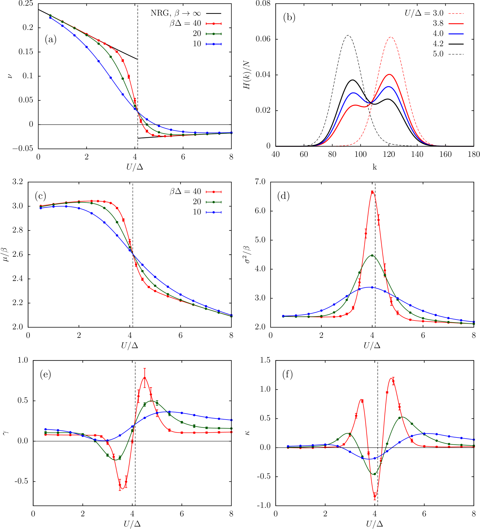
Figure 7: Same analysis as in Figs. 2-4 but for changing interaction strength $U$ for $\Gamma=\Delta$, $\varphi=0$ and $\varepsilon=0$ (half-filling): induced gap (panel a), histograms for $\beta\Delta=40$ in the vicinity of the critical point (b), average expansion order (c), variance (d), skewness (e) and excess kurtosis (f). Lines are splines of QMC data and serve only as a guide for the eye. The critical interaction strength $U_{c}\approx 4.12\Delta$ matches the available zero-temperature NRG data (solid black line in panel (a)).

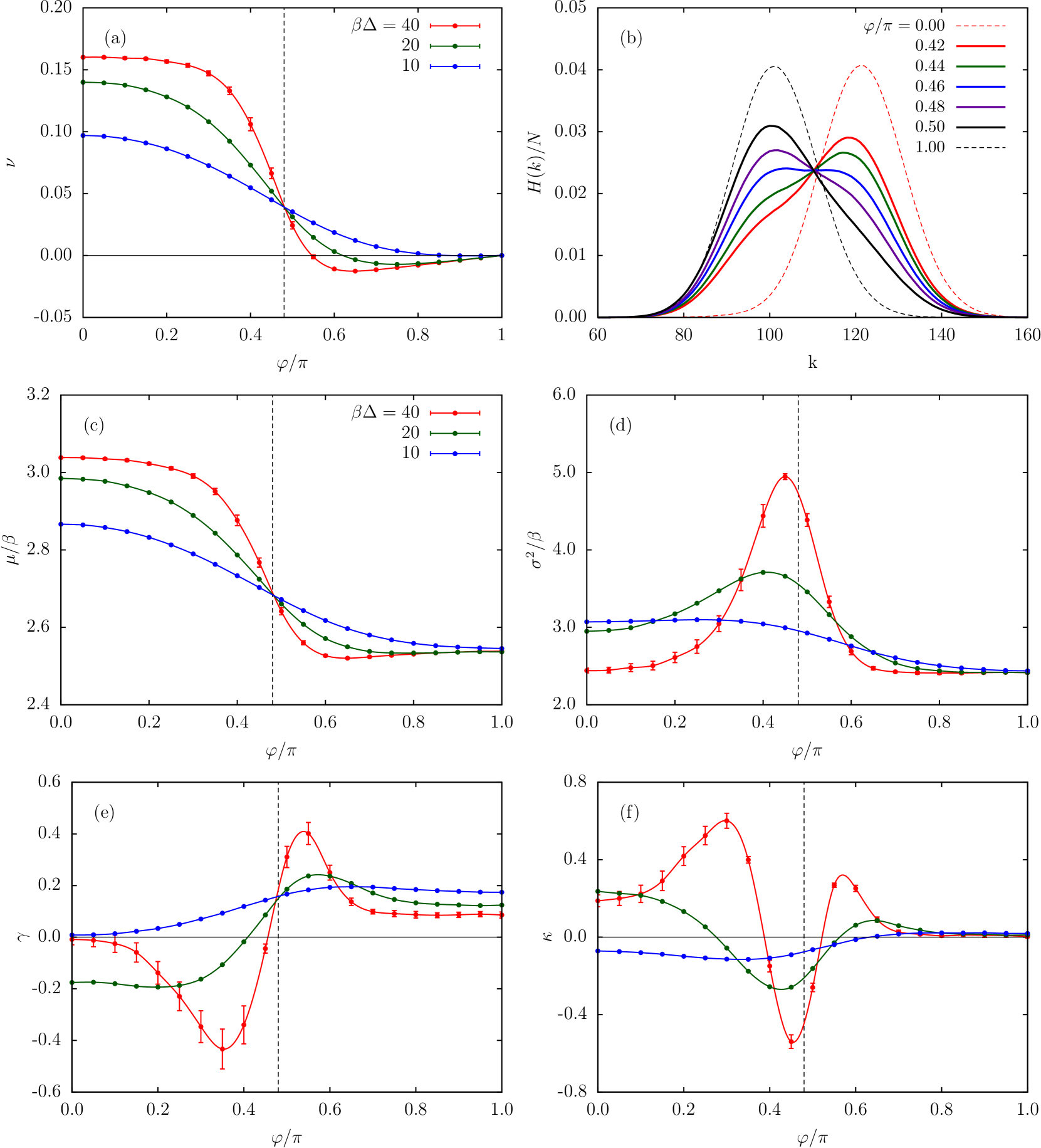
Figure 8: Same analysis as in Figs. 2-4 but for changing phase difference $\varphi$ for $U=3\Delta$, $\Gamma=\Delta$ and $\varepsilon=0$ (half-filling): induced gap (panel a), histograms for $\beta\Delta=40$ in the vicinity of the critical point (b), average expansion order (c), variance (d), skewness (e) and excess kurtosis (f). Lines are splines of QMC data and serve only as a guide for the eye. The critical phase difference $\varphi_{c}\approx 0.48\pi$ matches the available zero-temperature NRG data (not plotted).

References

- De Franceschi et al. [2010] S. De Franceschi, L. Kouwenhoven, C. Schönenberger, and W. Wernsdorfer, “Hybrid superconductor-quantum dot devices,” Nat. Nanotechnol. 5, 703–711 (2010).
- Martín-Rodero and Levy Yeyati [2011] A. Martín-Rodero and A. Levy Yeyati, “Josephson and Andreev transport through quantum dots,” Adv. Phys. 60, 899–958 (2011).
- Meden [2019] V. Meden, “The Anderson–Josephson quantum dot—a theory perspective,” J. Phys.: Condens. Matter 31, 163001 (2019).
- Luitz et al. [2012] D. J. Luitz, F. F. Assaad, T. Novotný, C. Karrasch, and V. Meden, “Understanding the Josephson current through a Kondo-correlated quantum dot,” Phys. Rev. Lett. 108, 227001 (2012).
- Bulla et al. [2008] R. Bulla, T. A. Costi, and T. Pruschke, “Numerical renormalization group method for quantum impurity systems,” Rev. Mod. Phys. 80, 395–450 (2008).
- Zalom et al. [2021] P. Zalom, V. Pokorný, and T. Novotný, “Spectral and transport properties of a half-filled Anderson impurity coupled to phase-biased superconducting and metallic leads,” Phys. Rev. B 103, 035419 (2021).
- Siano and Egger [2004] F. Siano and R. Egger, “Josephson current through a nanoscale magnetic quantum dot,” Phys. Rev. Lett. 93, 047002 (2004).
- Luitz and Assaad [2010] D. J. Luitz and F. F. Assaad, “Weak-coupling continuous-time quantum Monte Carlo study of the single impurity and periodic Anderson models with s-wave superconducting baths,” Phys. Rev. B 81, 024509 (2010).
- Domański et al. [2017] T. Domański, M. Žonda, V. Pokorný, G. Górski, V. Janiš, and T. Novotný, “Josephson-phase-controlled interplay between correlation effects and electron pairing in a three-terminal nanostructure,” Phys. Rev. B 95, 045104 (2017).
- Pokorný and Žonda [2018] V. Pokorný and M. Žonda, “Correlation effects in superconducting quantum dot systems,” Physica B 536, 488 – 491 (2018).
- Jarrell and Gubernatis [1996] M. Jarrell and J. E. Gubernatis, “Bayesian inference and the analytic continuation of imaginary-time quantum Monte Carlo data,” Phys. Rep. 269, 133–195 (1996).
- Maurand et al. [2012] R. Maurand, T. Meng, E. Bonet, S. Florens, L. Marty, and W. Wernsdorfer, “First order quantum phase transition in the Kondo regime of a superconducting carbon nanotube quantum dot,” Phys. Rev. X 2, 011009 (2012).
- Zanardi and Paunković [2006] P. Zanardi and N. Paunković, “Ground state overlap and quantum phase transitions,” Phys. Rev. E 74, 031123 (2006).
- Gu [2010] S.-J. Gu, “Fidelity approach to quantum phase transitions,” Int. J. Mod. Phys. B 24, 4371–4458 (2010).
- Albuquerque et al. [2010] A. F. Albuquerque, F. Alet, C. Sire, and S. Capponi, “Quantum critical scaling of fidelity susceptibility,” Phys. Rev. B 81, 064418 (2010).
- Rossini and Vicari [2018] D. Rossini and E. Vicari, “Ground-state fidelity at first-order quantum transitions,” Phys. Rev. E 98, 062137 (2018).
- Wang et al. [2015a] L. Wang, Y.-H. Liu, J. Imriška, P. N. Ma, and M. Troyer, “Fidelity susceptibility made simple: A unified quantum Monte Carlo approach,” Phys. Rev. X 5, 031007 (2015a).
- Huang et al. [2016] L. Huang, Y. Wang, L. Wang, and P. Werner, “Detecting phase transitions and crossovers in Hubbard models using the fidelity susceptibility,” Phys. Rev. B 94, 235110 (2016).
- Wang et al. [2015b] L. Wang, H. Shinaoka, and M. Troyer, “Fidelity susceptibility perspective on the Kondo effect and impurity quantum phase transitions,” Phys. Rev. Lett. 115, 236601 (2015b).
- Huang [2017] L. Huang, “iQIST v0.7: An open source continuous-time quantum Monte Carlo impurity solver toolkit,” Comput. Phys. Commun. 221, 423 – 424 (2017).
- Kadlecová et al. [2019] A. Kadlecová, M. Žonda, V. Pokorný, and T. Novotný, “Practical guide to quantum phase transitions in quantum-dot-based tunable Josephson junctions,” Phys. Rev. Applied 11, 044094 (2019).
- Kadlecová et al. [2017] A. Kadlecová, M. Žonda, and T. Novotný, “Quantum dot attached to superconducting leads: Relation between symmetric and asymmetric coupling,” Phys. Rev. B 95, 195114 (2017).
- van Dam et al. [2006] J. A. van Dam, Y. V. Nazarov, E. P. A. M. Bakkers, S. De Franceschi, and L. P. Kouwenhoven, “Supercurrent reversal in quantum dots,” Nature 442, 667–670 (2006).
- Cleuziou et al. [2006] J. P. Cleuziou, W. Wernsdorfer, V. Bouchiat, T. Ondarcuhu, and M. Monthioux, “Carbon nanotube superconducting quantum interference device,” Nat. Nanotechnol. 1, 53–59 (2006).
- Jørgensen et al. [2007] H. I. Jørgensen, T. Novotný, K. Grove-Rasmussen, K. Flensberg, and P. E. Lindelof, “Critical current transition in designed Josephson quantum dot junctions,” Nano Lett. 7, 2441–2445 (2007).
- Pillet et al. [2010] J.-D. Pillet, C. H. L. Quay, P. Morfin, C. Bena, A. Levy Yeyati, and P. Joyez, “Andreev bound states in supercurrent-carrying carbon nanotubes revealed,” Nat. Phys. 6, 965–969 (2010).
- Pillet et al. [2013] J.-D. Pillet, P. Joyez, R. Žitko, and M. F. Goffman, “Tunneling spectroscopy of a single quantum dot coupled to a superconductor: From Kondo ridge to Andreev bound states,” Phys. Rev. B 88, 045101 (2013).
- Li et al. [2017] S. Li, N. Kang, P. Caroff, and H. Q. Xu, “ phase transition in hybrid superconductor–InSb nanowire quantum dot devices,” Phys. Rev. B 95, 014515 (2017).
- Gull et al. [2011] E. Gull, A. J. Millis, A. I. Lichtenstein, A. N. Rubtsov, M. Troyer, and P. Werner, “Continuous-time Monte Carlo methods for quantum impurity models,” Rev. Mod. Phys. 83, 349–404 (2011).
- Haule [2007] K. Haule, “Quantum Monte Carlo impurity solver for cluster dynamical mean-field theory and electronic structure calculations with adjustable cluster base,” Phys. Rev. B 75, 155113 (2007).
- Merker and Costi [2012] L. Merker and T. A. Costi, “Numerical renormalization group calculation of impurity internal energy and specific heat of quantum impurity models,” Phys. Rev. B 86, 075150 (2012).
- Seth et al. [2016] P. Seth, I. Krivenko, M. Ferrero, and O. Parcollet, “TRIQS/CTHYB: A continuous-time quantum Monte Carlo hybridisation expansion solver for quantum impurity problems,” Comput. Phys. Commun. 200, 274–284 (2016).
- Žonda et al. [2016] M. Žonda, V. Pokorný, V. Janiš, and T. Novotný, “Perturbation theory for an Anderson quantum dot asymmetrically attached to two superconducting leads,” Phys. Rev. B 93, 024523 (2016).
- Yoshioka and Ohashi [2000] T. Yoshioka and Y. Ohashi, “Numerical renormalization group studies on single impurity Anderson model in superconductivity: A unified treatment of magnetic, nonmagnetic impurities, and resonance scattering,” J. Phys. Soc. Jpn. 69, 1812–1823 (2000).