A thorough study of the performance of simulated annealing in the traveling salesman problem under correlated and long tailed spatial scenarios

Abstract

Metaheuristics, as the simulated annealing used in the optimization of disordered systems, goes beyond physics, and the traveling salesman is a paradigmatic NP-complete problem that allows inferring important theoretical properties of the algorithm in different random environments. Many versions of the algorithm are explored in the literature, but so far the effects of the statistical distribution of the coordinates of the cities on the performance of the algorithm have been neglected. We propose a simple way to explore this aspect by analyzing the performance of a standard version of the simulated annealing (geometric cooling) in correlated systems with a simple and useful method based on a linear combination of independent random variables. Our results suggest that performance depends on the shape of the statistical distribution of the coordinates but not necessarily on its variance corroborated by the cases of uniform and normal distributions. On the other hand, a study with different power laws (different decay exponents) for the coordinates always produces different performances. We show that the performance of the simulated annealing, even in its best version, is not improved when the distribution of the coordinates does not have the first moment. However, surprisingly, we still observe improvements in situations where the second moment is not defined but not where the first one is not defined. Finite-size scaling fits, and universal laws support all of our results. In addition, our study show when the cost must be scaled.

1 Introduction

Some magnetic systems, known as spin glasses, present random couplings which lead to high levels of frustration and disordering. The metastability of many structures of such spin glasses leads to experimental physical measurements of the order of days due to slow decay of the magnetization to zero. This peculiarity is also hard to explore in computer simulations. Sherrington and Kirkpatrick [1] proposed an interesting exactly solvable spin-glass model that shows an slow dynamics of magnetization.

Based on these annealing phenomena (heating treatment of materials to enlarge its ductility) in solids, Kirkpatrick, Gelatt, and Vecchi [2] observed a deep connection between the Statistical Mechanics of systems with many degrees of freedom, which can be governed by the Metropolis prescription [3] to thermal equilibrium, and the combinatorial optimization of some problems related to obtain the minimal of functions with many parameters in complex landscapes.

Many combinatorial optimization problems belong to the complexity class known as NP-complete which is a subset of class simply known as NP class. Let us better explain this fundamental point in the complexity of algorithms. A problem belongs to the NP class if it can be decided in polynomial time by a Turing machine (a universal computer model, for more details see [4]). Here it is important to say that not necessarily it possesses an algorithm that can solve it in polynomial time. Sure, we know that there are problems which can be solved by an algorithm in polynomial time (fast solution) and not only decided! A simple example is sorting a list.

One algorithm in these conditions belongs to a complexity class known as P, and obviously P$\ \subset\$NP. However there are some ”rebel” problems in NP, the so-called NP-complete problems, that can be understood, in a non-rigorous way, as the harder problems in NP, since there is not a single known algorithm to date, that can solve one of these problems in polynomial time differently than occurs with problems in P.

Should we then believe in conjecture P$\ \neq\$NP? Yes, and the reason is simple! If we know one NP-complete problem, any algorithm that can solve it, can be used to solve any other NP-complete problem (this is technically called polynomial reduction, and for a good reference in complexity theory, see again [4]). Therefore, if somebody discovers an algorithm in polynomial time that solves one of these NP-complete problems, by consequence, all of them will also have solution in polynomial time. However, such algorithms were never found, which makes stronger the conjecture.

But what do you do with these problems? An alternative for them is to use heuristics, and those which are physically motivated can be a good option. Thus, based on Ref. [2], which proposed a metaheuristics known as simulated annealing (SA), an algorithm which performs a random walk in the configuration space until it reaches the global equilibrium or, at worst, an interesting local minimum, the physicists, and computer scientists have explored several different combinatorial problems, including for example the study of thermodynamics of the protein folding [5], the evaluation of periodic orbits of multi-electron atomic systems [6], and many others.

Basically, the SA algorithm works in the following way: we start with an initial solution/configuration $\sigma_{old}$, and calculate the energy (cost in a more general context) of this initial solution $E(\sigma_{old})$. After that, another state is randomly chosen, which is denoted by $\sigma_{new}$, and this new solution is accepted with a probability that follows the Metropolis prescription [3]:

$$\Pr(\sigma_{old}\rightarrow\sigma_{new})=\min\left\{1,\exp\left[-\frac{1}{T}\left(E(\sigma_{new})-E(\sigma_{old})\right)\right]\right\},$$ (1)

otherwise the system remains in the same $\sigma_{old}$ state. This process is repeated until the ensemble sampled of the system reaches an equilibrium at the given temperature. Finally, the temperature $T$ is decreased by a cooling schedule. The temperature will be decreased until a state with low enough energy is found.

Here, it is important to mention that many cooling schedules can be applied. There are cooling schedules that asymptotically converge towards the global minimum as the one that cools the system with a logarithm rule [7]. However such schedule converges very slowly and requires a long computation time.

There are good alternative schedules [8], that although without a rigorous guarantee of the convergence towards the global optimum, are computationally faster. One of them is the geometric cooling schedule [9] which considers that at time $t$, the temperature is given by $T=\alpha^{t}T_{0}$, with $0<\alpha<1$. An interesting version of this heuristic works with two loops: an internal and another external which can be resumed by the Heuristic SAGCS (Simulated annealing with geometric cooling schedule) resumed in the algorithm 1.

parameters :  $\sigma_{0}$ : initial configuration

$T_{0}$ : initial temperature

$T_{\min}$ : final temperature

$N_{iter}$ : number of iterations of the internal loop

$\alpha$ : coefficient of the geometric cooling

Result: low energy state $\sigma$

$T\leftarrow T_{0}$;

$\sigma\leftarrow\sigma_{0}$;

while $T>T_{\min}$ do

       for $i\leftarrow 1$ to $N_{iter}$ do

             $\sigma_{new}\leftarrow\textnormal{{randomState(}}\textnormal{\emph{}}\textnormal{{)}}$;

             if $E(\sigma_{new})<E(\sigma)$ then

                   $\sigma\leftarrow\sigma_{new}$;

                  

            else

                   $x\leftarrow\textnormal{{rand(}}\textnormal{\emph{$[0,1]$}}\textnormal{{)}}$;

                   if $x<\exp{\left[-\frac{1}{T}(E(\sigma_{new})-E(\sigma))\right]}$ then

                         $\sigma\leftarrow\sigma_{new}$;

                        

                   end if

                  

             end if

            

       end for

      $T\leftarrow\alpha T$;

      

end while

Algorithm 1 SAGCS (Standard Simulated Annealing with Geometric Cooling Schedule)

It is important to observe that such Heuristic works with two parameters: $N_{iter}$ that controls the number of internal iterations, while the external loop (iterations over different temperatures) is governed by:

$$N_{steps}=\left\lfloor\frac{\ln(T_{\min}/T_{0})}{\ln\alpha}\right\rfloor$$ (2)

and sure, for appropriate $N_{steps}$ and $N_{iter}$, the system must converge for a local minimum that is very close to the global minimum. Amongst the many interesting NP-complete problems, the traveling salesman problem (TSP) deserves much attention and it became a natural way to test the SA heuristic using different cooling schedules, variations of the method, and parallelization techniques in many different contexts (see for example [7, 8, 9, 12, 13, 14, 15]). The problem (TSP) is to find the optimal Hamiltonian cycle on a given graph (vertices and valued edges), i.e., the minimum cost closed path including all vertices passing through each vertex only once.

Let us consider graphs with $N$ vertices corresponding to points $(x_{i},y_{i})$, $i=1,..,N$, distributed in a two dimensional scenario. In this case, the graph naturally has valued edges defined by the Euclidean distances:

$$d(i,j)=\sqrt{(x_{i}-x_{j})^{2}+(y_{i}-y_{j})^{2}},$$ (3)

with $i,j=1,..,N$, and therefore, the simplest situation is to consider the graph having all edges, since all costs $d(i,j)$ can be defined for all pair of the points, which is denoted by a complete graph.

In this paper, we are not interested in testing cooling schedules, or even other SA heuristics, which are very well explored in the literature, but in building computer experiments to test the SAGCS in the TSP in order to understand its efficiency considering the effects of correlation and variance on the random coordinates $x_{i}$ and $y_{i}$. It is important to mention that our method to include correlation is very simple and allows to change the correlation but keeping the same variance which is very important for making a fair comparison, since we simultaneously variate the two parameters, we do not know if the effects are only caused by the correlation.

Our results show how the performance of the algorithm transits from two-dimensional scenario ($\rho=0$) to the one-dimensional situation ($\rho=1$) by deforming the region where the points (cities) are distributed. Here $\rho$ is the correlation coefficient between the coordinates of the points. We also investigate a parameter that controls the moments of the random variables $x_{i}$ and $y_{i}$ and we quantitatively show how the increase of the variance affects the performance. We particularly show that the shape of the distribution is more important than its variance in certain situations. On the other hand, when the points have coordinates that are power-law distributed, in the region where the average cannot be defined, the efficiency of the algorithm is negligible independently on scaling.

In the next section we will show some fundamental and pedagogical aspects of the SA for the TSP. In the following, in section 3 we define the different environments where we will apply the SAGCS. We will show in detail how to generate points with correlated coordinates, and how to generate points with power-law distributed coordinates. In section 4 we show our results and finally in section 5 we present some conclusions.

2 Pedagogical aspects of the Simulated Annealing in the context of the Travelling salesman problem

The simulated annealing with geometric schedule (SAGCS) is a very simple heuristic used to optimize combinatorial problems as the Traveling Salesman Problem. The points $(x_{i},y_{i})$, with $i=1,...,N$ are scattered over a two dimensional region, where the coordinates follow some joint probability distribution $p(x_{i},y_{i})$.

Denoting by $v(i)\equiv(x_{i},y_{i})$ the $i$-th point of the cycle $\sigma\equiv$ $v(1)\rightarrow v(2)\rightarrow....\rightarrow v(N-1)\rightarrow v(N)\rightarrow v(1)$, whose cost is given by

$$C=E(\sigma)\sum_{k=1}^{N}d(v(k),v(k+1))$$ (4)

where $v(N+1)=v(1)$ and $d(i,j)$ is given by Eq. 3. We aim to determine the best cycle $\sigma$, i.e., the cycle of minimal cost.

The new configuration can be obtained performing different mechanisms in this work. The first one is the “simple swap”(SS) , i.e., a point is randomly chosen, for example $v(j)$, and the candidate to be the new configuration $\sigma^{\prime}\$corresponds to $\sigma$ by simply changing the positions of $v(j)\equiv(x_{j},y_{j})$ and $v(j+1)\equiv(x_{j+1},y_{j+1})$, then we can perform the Metropolis prescription to optimize the problem in the context of the simulated annealing.

On the other hand, there is a more interesting way to obtain a new configuration according to [10, 11] the 2-opt move. It is a popular procedure used to improve algorithms to approximate the solution of the Travelling Salesman Problem. Starting from a given cycle, it consists in exchanging two links of the cycle to construct a new one. This is performed by reversing the sequence of nodes between the selected links and then reconnecting the cycle back together. For example, if one has a route/cycle $\sigma\equiv v(1)\rightarrow v(2)\rightarrow v(3)\rightarrow v(4)\rightarrow v(5)\rightarrow v(6)\rightarrow v(7)\rightarrow v(8)\rightarrow v(1)$, by choosing $i=4$ and $i=7$, it leads to $\sigma^{\prime}\equiv v(1)\rightarrow v(2)\rightarrow v(3)\rightarrow v(7)\rightarrow v(6)\rightarrow v(5)\rightarrow v(4)\rightarrow v(8)\rightarrow v(1)$. It allows us to explore the state space of Hamiltonian cycles efficiently as well as it provides a simple way to calculate the energy difference between the states before and after the move, which is a very important feature for working in conjunction with the Metropolis algorithm.

Now, let us explore the complexity of the problem. There are $N!$ different cycles. Testing all of them is impossible for large $N$! For example for $N=2048$ cities (this will be a number of cities of the most of our examples), by using the Stirling’s formula $N!\approx\sqrt{2\pi}N^{N+1}e^{-N}$, one estimates

$$2048!\approx\sqrt{2\pi}2048^{2048+1}e^{-2048}\approx 7.57\times 10^{5895}$$

This a staggering number when compared, for example, with the number of atoms of the universe $O(10^{80}$). Actually, among this ”astronomical” number of different cycles (much more than astronomical), certainly there are a lot of them corresponding to a good local minima. It is exactly here that SA shows its usefulness. Let us understand how it works by showing the power of this algorithm. For example, let us examine the Fig. 1.

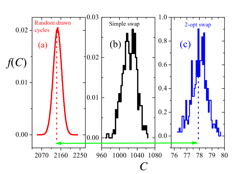
Figure 1: The reason for that the SA is so important. We show the histogram of the costs of the 10⁶ random drawn cycles (a), 400 different runs of the SA using simple swap (b), and 400 different runs of the SA using 2-opt choice for new configurations (c). The line green is only to highlight the huge difference between our best result obtained with SA and the “brute force sampling”

This figure shows three histograms: the red one, represented in Fig. 1 (a) shows a sample of the costs of one million of random drawn cycles of the same configuration with $N=2048$ cities, denoting points whose coordinates are randomly distributed according to a uniform distribution, with $x_{i}\in[-1,1]$ and $y_{i}\in[-1,1]$. The black one, Fig. 1 (b), represents a histogram with only 400 different costs obtained from $N_{run}=400$ different random configurations of $N=2048$ of the SAGCS with simple swap (SS-SAGCS), by considering $T_{0}=10$, $T_{\min}=10^{-5}$, $\alpha=0.99$, and $N_{iter}=8000$.

One can observe two very distinct Gaussian distributions whose means differ across 1000 units of the cost. It is important to notice that not even one among the one million costs of randomly drawn Hamiltonian cycles reached the cost of SA. Actually, it is worse than this, in the first case we have $\overline{C}_{rand}=2143.74\pm 0.02$, while in the second case one has $\overline{C}_{SA}=1021.67\pm 0.74$ and the overlapping probability between these two distributions is zero in the precision of the any known machine! It is important to mention that we provocatively used only $N_{run}=400$ runs for the SA against the brute force (random drawn cycles).

The final blow comes when we use the 2-opt choice to sample new configurations in the SAGCS (2opt-SAGCS), which is shown Fig. 1 (c), where we exactly used the same parameters of the Fig. 1 (b). In this case one has $\overline{C}_{SA}=77.959\pm 0.031$ which is an extremely low cost when compared with brute force method.

Thus, this pedagogical explanation is only to show that exhaustive sampling is not a feasible solution for combinatorial problems. Heuristics as the SA are an important alternative to obtain good (not always the optimal, but in very disordered systems this is not be a meaningful difference) solutions to the TSP. Now, after this preparatory study, we present the details about the scenario for which we intend to analyze the performance of the SAGCS. In the next section we will present the method to generate points with correlated coordinates, and how to generate points with coordinates long-tailed distributed. In these environments, we intend to explore some effects on the performance of the SA which will be performed in section 4.

3 Correlated and long-tailed environments

One of the important questions addressed in this paper is how the SAGCS works considering that $x_{i}$ and $y_{i}$, the coordinates of the cities, are random variables with a given correlation $\rho$. Additionally, for the particular case $p(x_{i},y_{i})=p(x_{i})p(y_{i})$ ($\rho=0$), we also study the performance of SAGCS for distributions $p(x_{i})\sim x_{i}^{-\gamma}$ and $p(y_{i})\sim y_{i}^{-\gamma}$, looking at the effect of $\gamma$ on performance of the algorithm. Now, we discuss how to generate scenarios by following these prescriptions.

3.1 Generating correlated random coordinates from non-correlated random variables

In this section, we will show that we can generate correlated random variables from non-correlated random variables considering that both (correlated and non-correlated) have the same variance and average by imposing an additional constraint – considering the average equal to 0 for the uncorrelated random variables. This is exactly the same procedure used in [16] in the context of emerging of rogue waves in the superposition of electrical waves with correlated phases.

Let us consider spatial coordinates $x$ e $y$ of points (our cities) in a two-dimensional environment that are random variables:

$$\begin{array}[]{ccc}x&=&\alpha_{1}z_{1}+\alpha_{2}z_{2}\\ &&\\ y&=&\beta_{1}z_{1}+\beta_{2}z_{2}\end{array}$$ (5)

where $z_{1}$ and $z_{2}$ are independent and identically distributed random variables, such that: $\left\langle z_{1}\right\rangle=\left\langle z_{2}\right\rangle=\left\langle z\right\rangle$, and $\left\langle z_{1}z_{2}\right\rangle=\left\langle z_{1}\right\rangle\left\langle z_{2}\right\rangle=\left\langle z\right\rangle^{2}$.

The variance of the variable $x$ is given by:$\ \left\langle\left(\Delta x\right)^{2}\right\rangle=\left\langle x^{2}\right\rangle-\left\langle x\right\rangle^{2}=(\alpha_{1}^{2}+\alpha_{2}^{2})\left\langle\left(\Delta z\right)^{2}\right\rangle$ where $\left\langle z_{1}^{2}\right\rangle-\left\langle z_{1}\right\rangle^{2}=\left\langle z_{2}^{2}\right\rangle-\left\langle z_{2}\right\rangle^{2}=\left\langle z^{2}\right\rangle-\left\langle z\right\rangle^{2}=\left\langle\left(\Delta z\right)^{2}\right\rangle$, and similarly $\left\langle\left(\Delta y\right)^{2}\right\rangle=(\beta_{1}^{2}+\beta_{2}^{2})\left\langle\left(\Delta z\right)^{2}\right\rangle$.

Now, we impose the condition

$$\left\langle\left(\Delta x\right)^{2}\right\rangle=\left\langle\left(\Delta y\right)^{2}\right\rangle=\left\langle\left(\Delta z\right)^{2}\right\rangle,$$ (6)

which implies that $\alpha_{1}^{2}+\alpha_{2}^{2}=\beta_{1}^{2}+\beta_{2}^{2}=1$.

It is worth noting that although $z_{1}$ and $z_{2}$ are non-correlated random variables, $x$ and $y$ are, and the correlation between these random variables can be calculated:

$$\rho=\frac{\left\langle\left(\ x-\left\langle x\right\rangle\right)\left(\ y-\left\langle y\right\rangle\right)\right\rangle}{\sqrt{\left\langle\left(\Delta x\right)^{2}\right\rangle\left\langle\left(\Delta y\right)^{2}\right\rangle}}$$ (7)

Thus, again after some cancellations and combinations: $\rho=(\alpha_{1}\beta_{1}+\alpha_{2}\beta_{2})$. And after a little algebra, the random variables can be now written as:

$$x=\sin\left(\frac{1}{2}\sin^{-1}(\rho)\right)z_{1}+\cos\left(\frac{1}{2}\sin^{-1}(\rho)\right)z_{2}$$ (8)

and

$$y=\cos\left(\frac{1}{2}\sin^{-1}(\rho)\right)z_{1}+\sin\left(\frac{1}{2}\sin^{-1}(\rho)\right)z_{2}$$ (9)

have the same average that are given by:

$$\begin{array}[]{ccccc}\left\langle x\right\rangle&=&\left\langle y\right\rangle&=&\frac{1}{\sqrt{2}}\left[\left(1-\sqrt{1-\rho^{2}}\right)^{1/2}+\left(1+\sqrt{1-\rho^{2}}\right)^{1/2}\right]\left\langle z\right\rangle\end{array}$$

From this, we can draw two important conclusions:

1. The random variables $x$ and $y$ have the same variance of $z_{1}$ and $z_{2}$ that are identically distributed and we required this according to Eq. 6 and therefore it does not depend on $\rho$;

2. If $\left\langle z_{1}\right\rangle=\left\langle z_{2}\right\rangle=\left\langle z\right\rangle=0$, then $\left\langle x\right\rangle=\left\langle y\right\rangle=0$.

Thus, if one considers $x$ and $y$ as $\rho$-correlated random variables generated from two independent random variables $z_{1}$ and $z_{2}$, with average zero and variance $\sigma^{2}=\left\langle\left(\Delta z\right)^{2}\right\rangle$, $x$ and $y$ also have average zero and the same variance $\sigma^{2}$. This is an important point because if one works with different averages and dispersions between the cases $\rho=0$ and $\rho\neq 0$ the results can be misleading since there will be no parameter for a fair comparison, i.e., in our problem no bias can be the source of the possible studied effects, since independently on correlation, the random variables are sampled with the same average and variance.

Figure 2: Effects of correlation on the points using Eqs. 8 and 9.

For example, using two uniform and identically distributed random variables $z_{1}=2(\xi_{1}-\frac{1}{2})$ and $z_{2}=2(\xi_{2}-\frac{1}{2})$ that assume values in $[-1,1]$ generated from two $\xi_{1}$ and $\xi_{2}$ uniform random variables assuming values in $[0,1]$, the Fig. 2 shows a plot of $y$ versus $x$ obtained from equations 8 and 9 for different values of $\rho$. In this paper, the idea is to study the SAGCS on these correlated scenarios by analyzing its performance.

3.2 Power-law distributions for the coordinates

Another important point of our study is to look at the effects of long tailed distributions for the coordinates of the points on the SA performance. Thus, we use a power-law probability density function to generate the coordinates of the two-dimensional points. For that, we initially propose the following distribution for the coordinates:

$$p(x;x_{0},\gamma)=\left\{\begin{array}[]{cc}\frac{(\gamma-1)}{2x_{0}^{1-\gamma}}\left|x\right|^{-\gamma}&\text{if\ }\left|x\right|\geq x_{0}\\ &\\ 0&\text{otherwise}\end{array}\right.$$ (10)

It is important to observe that the power law distribution given by Eq. 10 has a necessary gap $\Delta=2x_{0}$ with center in the origin, since the two branches can not touch the origin by normalization, however $x_{0}$ can be made arbitrarily small. Just for illustration, we show plots of $p(x;x_{0},\gamma)$ in Fig. 3.

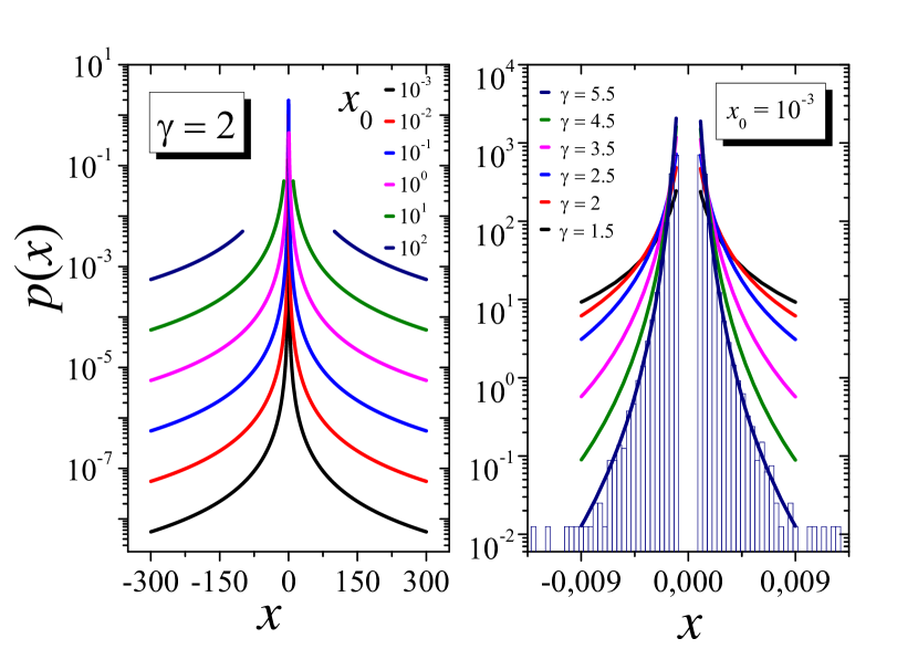
Figure 3: Two-tailed power law distribution. Fig. (a): A plot of $p(x;x_{0},\gamma)$ for $\gamma=2$ and different values of $x_{0}$. Fig. (b): A plot of $p(x;x_{0},\gamma)$ for $x_{0}=10^{-3}$ for different values of $\gamma$. The histogram is obtained with points sampled with Eq. 11 for $\gamma=5.5$, only to check the formulae.

In order to draw a variable that follow the distribution of Eq. 10 one simply uses two uniform random (or more precisely pseudo-random variables) variables $\xi_{1}$ and $\xi_{2}$ assuming values in $[0,1]$. First, one chooses if the variable is on the positive or negative branching. This is performed checking the sign of $(2\xi_{1}-1)$. After that, one makes $\xi_{2}$ equal to area $\frac{(\gamma-1)}{x_{0}^{1-\gamma}}\int_{x_{0}}^{w}x^{-\gamma}dx$. This results in $w=x_{0}(1-\xi_{2})^{\frac{1}{1-\gamma}}$. Therefore, in the general case, the random variable built from $\xi_{1}$ and $\xi_{2}$ is:

$$x=\frac{2\xi_{1}-1}{\left|2\xi_{1}-1\right|}x_{0}(1-\xi_{2})^{\frac{1}{1-\gamma}}$$ (11)

and naturally with other two random variables $\xi_{3}$ and $\xi_{4}$, which are chosen from the uniform distribution in [0, 1], one has

$$y=\frac{2\xi_{3}-1}{\left|2\xi_{3}-1\right|}x_{0}(1-\xi_{4})^{\frac{1}{1-\gamma}}$$ (12)

In Fig. 3 (b), a histogram for the points $(x,y)$ sampled in this way is shown for $\gamma=5.5$, only to check the agreement with the exact result. The idea is to observe the performance of the SAGCS in this scenario answering how important is $\gamma$ and its effects on the final cost obtained with SA algorithm. Notice that points generated by Eqs. 11 and 12 have border effects. For instance, in Fig. 4, we present some examples of the points scattered according to different distributions by focusing the power law ones.

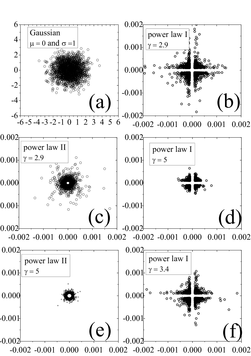
Figure 4: Scattering of points for a comparison: (a) Gaussian coordinates, (b-e) power-law coordinates for different approaches and for different exponents $\gamma$. It is important to notice that the figures are shown with different intervals for a good visualization. We used both $x_{0}$ (power law I) and $r_{0}$ (power law II) equal to $10^{-3}$.

Using the Gaussian distribution (with average zero and variance 1), the pattern of points shown in Fig. 4 (a) is very different than the case which uses the points generated by Eqs. 11 and 12 for $\gamma=2.9$ and $x_{0}=10^{-3}$ (Fig. 4 (b) ). Here, we will denote the points using the Eqs. 11 and 12 by power law I. We can observe some outlier points since, for this case, the distribution has no second moment defined. However, radial symmetry is absent in the power law I distribution and the border effects previously mentioned are notorious. The question is whether they are really important. Alternatively, in this paper, we also proposed a second power law type (power law II) to study the SA, which respects the radial symmetry:

$$x = r_{0}(1-\xi_{1})^{\frac{1}{1-\gamma}}\cos(2\pi\xi_{2})$$ (13)

$$y = r_{0}(1-\xi_{1})^{\frac{1}{1-\gamma}}\sin(2\pi\xi_{2})$$

and in this case for $\gamma=2.9$ and $r_{0}=10^{-3}$ one has the distribution of points represented in Fig. 4 (c). Similarly $\xi_{1}$ and $\xi_{2}$ are uniform random variables assuming values in $[0,1]$. Thus relevant questions should be related to the performance of the SA in both situations: radially symmetric and asymmetric ones. By completing in Fig 4 (d), and (e) we show the distribution of points for a case where we have defined variance ($\gamma=5.5$) and therefore few outliers are observed. The case $\gamma=3.4$ complete our figure (Fig 4 (f) ) since this case will be particularly important for our results. It is important to mention that except by Fig. 4 (a) where the range used was $-4\leq x,y\leq 4$, all other Figs. 4 (b), (c), (d), (e), and (f) that correspond to power-law cases, we used the range $-0.002\leq x,y\leq 0.002$ for a suitable visualization and comparison.

4 Results

We performed computer experiments to analyze two effects on the optimization by the SA for the TSP: a) the correlation between the spatial coordinates, and b) the variance/distribution shape for the spatial random coordinates. We used the SAGCS which is a fast and standard way to perform optimization. It is natural to expect that such effects must be proportionally important in other variations of the SA employing other slower cooling schedules independently if the final cost obtained is better. The goal of this paper is not to compare different SA algorithms but performing a quantitative study of the SAGCS considering different spatial distributions for the coordinates of the points in the TSP.

However, before starting the main core of our results, it is important to understand some preliminary aspects: the effects of the number of external loop iterations $N_{steps}=\left\lfloor\frac{\ln(T_{\min}/T_{0})}{\ln\alpha}\right\rfloor$, and $N_{iter}$ which denotes the number of internal loop iterations on the final cost. We consider points $(x_{i},y_{i})$, $=1,...,N$ uniformly distributed non-correlated random variables (case $\rho=0$ in Fig. 2). In all of our simulations, we averaged our final cost over $N_{run}=60$ different runs of the SA.

So we performed simulations considering $T_{0}=10$ and $T_{\min}=10^{-5}$. We initially consider the simple swap scheme to generate new candidate configurations. Under these conditions, one obtains a plot of the cost in the steady state ($C_{opt}$) which can be observed in Fig. 5 (a) as function of total number of iterations $N_{total}=N_{steps}N_{iter}$. Here we intent to show that such parameter is more important than the parameters $N_{steps}(\alpha)$, and $N_{iter}$ separately. Our range for $N_{total}$ was from $5.10^{5}$ iterations up to $10^{9}$ iterations. The procedure is to change $N_{iter}$ from $2^{10}$ up to $2^{18}$. Now, given the $N_{total}$ and the $N_{iter}$ we obtain the factor of the exponent $\alpha$ of the cooling:

$$\alpha=\left\lfloor\left(\frac{T_{\min}}{T_{0}}\right)^{\frac{N_{iter}}{N_{total}}}\right\rfloor$$

For example, when $N_{total}=5.10^{5}$, $\alpha$ changes from $0.001$ up to $0.9734$ and when $N_{total}=2.10^{9}$ one obtains that $\alpha$ changes from $0.99831$ up to $0.99999$. There is actually a lot of information aggregated in this figure to grasp. First the size of the points is proportional to $N_{iter}$ and $\alpha\rightarrow 0$ corresponds to red, while $\alpha\rightarrow 1$ corresponds to blue.

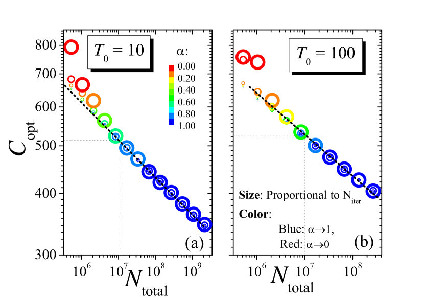
Figure 5: Final cost (steady state cost) as function of $N_{total}=N_{steps}\cdot N_{iter}$. The color denotes the different values of $\alpha$ while the size of the points is proportional to $N_{iter}$.

Fig. 5 shows that $C_{opt}$ depends on $N_{total}$ and not on $N_{steps}$ and $N_{iter}$ separately. For this experiment it was used $N=2048$ cities. The 5 (b) shows that for $T_{0}=100$ the behavior is similar. The result suggests a reasonable power-law universal behavior

$$C_{opt}\sim N_{total}^{-\delta}$$

for sufficiently large total number of points in the sample independently on the internal or external loops. For clarity, in the Fig. 6, we show a plot of $C_{opt}$ as function of $N_{total}$ for both $T_{0}=10$ and $T_{0}=100$ in the same plot, forgetting at this moment the effects of $\alpha$ and $N_{iter}$ separately. In log-log scale we obtain respectively $\delta=0.079\pm 0.001$ and $\delta=0.083\pm 0.001$, which shows a similar power law behavior.

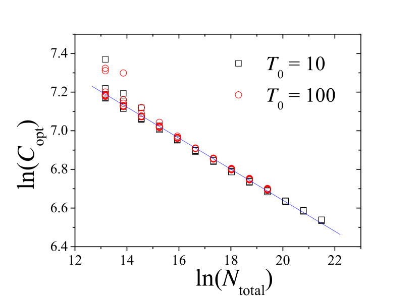
Figure 6: Highlighting the power law behavior of the final cost as function of $N_{total}$ discarding the effects of $N_{iter}$ and $\alpha$ separately for both cases: $T_{0}=10$ and $T_{0}=100$. We can observe that both curves have similar power law behaviors, where the obtained exponents were $\delta=0.079\pm 0.001$ and $\delta=0.083\pm 0.001$ respectively.

We perform a similar analysis of Fig. 6 for the 2-opt prescription, which is shown in Fig. 7. In this case, somewhat differently from the simple swap, one observes a transition between two power laws with very different exponents: from $\delta\approx 0.43$ transiting to $\delta\approx 0.02$, which shows that for $N_{total}>O(e^{16})\sim O(10^{6})$ the optimal cost found does not show a meaningful improvement, by changing from $C_{opt}\approx 90$ up to $C_{opt}\approx 70$. After this preparatory study, we can proceed to the main study of this work, to investigate the correlation and long range effects on the coordinates of the points.

4.1 Correlation effects

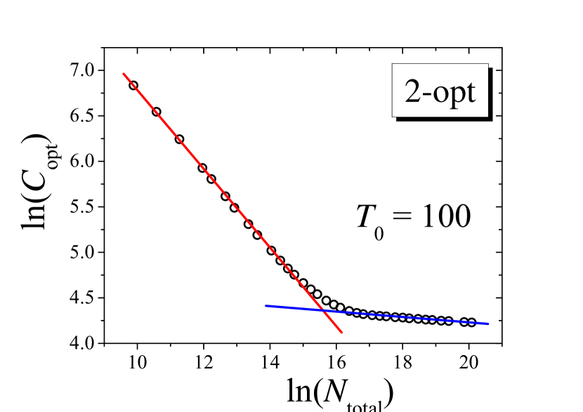
Figure 7: Power law behavior of the final cost as function of $N_{total}$ for the prescription 2-opt exactly as performed in Fig. 6 for the simple swap. One observes a transition from $\delta\approx 0.43$ to $\delta\approx 0.02$.

From now, all of our results were obtained by using a fixed set of parameters $N_{iter}=8000$, $\alpha=0.99$, $N_{run}=60$, $T_{\min}=10^{-5}$, and $T_{0}=10$, which results in $N_{total}=O(10^{7})$. Except by the finite size scaling analysis, all of our experiments with SAGCS were applied in scenarios with $N=2048$ cities.

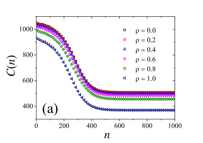
Figure 8: Plot (a): Time evolution of the cost $C(n)$. Here $n$ is the iteration of the external loop (cooling schedule) Plot b-I: Performance of the SA as function of $\rho$ for different number of cities. Plot b-II An approximate scaling for the plot (b-I). One used simple-swap prescription to generate new configurations in both plots.

Let us start our study of correlation effects, by observing the behavior of $C$ as function of the iteration in the external loop (iteration of cooling schedule) $n$, for different values of $\rho$ in scenarios with cities/points ($x$,$y$) built from identical uniform random variables $z_{1}$ and $z_{2}$ defined on [-1,1] as the Fig. 2. We will first study the SS-SAGCS performance.

In Fig. 8(a) we can observe a decreasing of the final cost $C_{opt}$ until it reaches a steady state after approximately 500 iterations. However, an interesting analysis is to consider the ratio $\overline{C_{opt}}/\overline{\left\langle C\right\rangle}$, given by

$$\left\langle C\right\rangle=N\frac{\sum_{i<j}d(i,j)}{\binom{N}{2}}=\frac{2}{(N-1)}\sum_{i<j}d(i,j),$$ (14)

where the average cost is calculated considering that cities have an average distance multiplied by the size of cycle, and here, $\overline{O}=(1/N_{run})\sum_{i=1}^{N_{run}}O_{i}$ denotes an average of amount $O$ over the different runs (different steady costs obtained by the SA). It is important to say that $\left\langle C\right\rangle$ calculated by Eq. 14 has no difference of the cost of any cycle which was randomly chosen. This is a typical characteristic of the TSP, since Hamiltonian cycles randomly generated are so far from the local minimum found by heuristics as the SA, that even generating billions of such cycles, the probability of reaching a good local minimum as the SA can be disregarded as we previously discussed in Sec. 2.

The lower $C_{opt}/\left\langle C\right\rangle$, the better the performance. Fig. 8 (b-I) shows the behavior of this ratio as function of $\rho$ for several different values of $N$. We have an improvement of the performance as $\rho$ enlarges. A reasonable (not so good) empirical scaling can be observed in Fig. 8(b-II). If one uses $b=L_{\max}/L$ and adjust $z\approx 0.075$, the different curves have a good agreement in the collapse. Here $L_{\max}$ is the largest lattice size used in such study, which was $L_{\max}=2^{11}$.

We can observe that the performance for SS-SAGCS is even better for small number of cities for the simple swap prescription. But, an important point is to better investigate the performance of the SAGCS as function of $\rho$. Let us focus the extreme cases: $\rho=0$ and $\rho=1$. For $\rho=1$, one has exactly the points scattered in a straight line (case $\rho=1$, Fig. 2). In this particular case, we know in advance, the global optimal Hamiltonian cycle, which is exactly given by $C_{glob}^{(theor)}=4\sqrt{2}$ when $N\rightarrow\infty$, since we have points increasingly closer to $(-1,-1)$ and $(1,1)$ the higher the value of $N$, and therefore for finite $N$ is only an approximation. On the other hand, we can analytically estimate the averaged cycle

$$\begin{array}[]{lll}\left\langle C\right\rangle_{\rho=1}^{(theor)}&=&\frac{2N}{N(N-1)}\sum_{i<j}^{N}d(i,j)\\ &&\\ &\approx&\frac{2N}{N(N-1)}\sum_{j=1}^{N-1}\sum_{i=1}^{N-j}i\left\langle\Delta\right\rangle\end{array}$$

where $\left\langle\Delta\right\rangle$ $=\frac{4\sqrt{2}}{N}$ is the average displacement between two adjacent pair of points which is randomly distributed over the line. Thus,

$$\begin{array}[]{lll}\left\langle C\right\rangle_{\rho=1}^{(theor)}&=&\frac{8\sqrt{2}}{N(N-1)}\sum_{j=1}^{N-1}\sum_{i=1}^{N-j}i\\ &&\\ &=&\frac{4\sqrt{2}}{3(N-1)}(N^{2}-1)\\ &&\\ &=&\frac{4\sqrt{2}}{3}(N+1)\end{array}$$

Precisely:

$$C_{glob}^{(theor)}(\rho=1)/\left\langle C\right\rangle_{\rho=1}^{(theor)}=\frac{3}{(N+1)}\text{.}$$

which leads to the ratio $C_{glob}^{(theor)}/\left\langle C\right\rangle_{\rho=1}^{(theor)}=\frac{3}{2049}\approx 0.001\,5$, for $N=2048$. This shows that $C_{glob}$ is around of $O(10^{-3})$ smaller than $\left\langle C\right\rangle_{\rho=1}^{(theor)}$, however the SA finds $\overline{C}_{opt}^{(SS)}/\overline{\left\langle C\right\rangle}\approx 0.38$ which is a modest reduction. But one uses simple swap and such modest reduction is indeed expected. What about 2-opt? With the same parameters, and using this prescription, should the reduction of $O(10^{-3})$ be expected? Yes, as it can be observed in Table 1, which shows a comparison of $C_{opt}$ for different values of $\rho$. One observes that $C_{opt}^{(2-opt)}$, the cost obtained with 2-opt-SAGCS is smaller than $C_{opt}^{(SS)}$ (the one obtained with SS-SAGCS) and the difference is huge indeed.

Thus, considering the estimate for $\rho=1$, one obtains $\overline{C}_{opt}^{(2-opt)}/\overline{\left\langle C\right\rangle}\approx\allowbreak 0.002$ which leads to a very similar measure when compared with the one obtained by analytical means.

$\rho$	0	0.2	0.4	0.6	0.8	1.0
Simple Swap: $\overline{C}_{opt}^{(SS)}$	1020.4(7)	1014.5(7)	997.9(7)	965.6(7)	909.5(7)	735.8(9)
2-Opt: $\overline{C}_{opt}^{(2-opt)}$	77.94(3)	77.18(3)	74.72(3)	69.90(3)	60.82(2)	7.873(4)

Table 1: Comparison between the simple swap and 2-opt prescriptions in the SAGCS for the final average costs as function of $\rho$

Actually, finding the optimal Hamiltonian cycle with points scattered in a straight line is equivalent to order a list and one has good algorithms in polynomial times (heapsort, quicksort…) that efficiently performs such classification.

Nevertheless, it is important to mention that we have no previous information about the topology of the points and the simulated annealing with 2-opt prescription simply works to find a similar result to the optimal one for $\rho=1$ as well as in any other situation, which is very interesting indeed.

Let us analyze the ratio $C_{glob}/\left\langle C\right\rangle_{\rho=0}$ to check if the curve $C_{opt}/\left\langle C\right\rangle$ $\times\rho$ obtained with SA is compatible with these extremes. Once $C_{glob}$ for $\rho=0$ is not known, how do we estimate $C_{glob}/\left\langle C\right\rangle_{\rho=0}$? First, let us start with a calculation that can be performed exactly (see Appendix):

$$\left\langle C\right\rangle_{\rho=0}^{(theor)}=\frac{2N}{15}(2+\sqrt{2}+5\ln(\sqrt{2}+1))$$

which amounts to $2136$, approximately, for $N=2048$. Just to check, for $N_{run}=60$, we numerically obtain $\overline{\left\langle C\right\rangle}_{\rho=0}\approx 2131$. Although we do not exactly know $C_{glob}$, constructive heuristics (out of scope of the Boltzmann machines) can supply an estimate which should work as a benchmark. A good suggestion is the nearest neighbor (NN) algorithm [17], a greedy algorithm that corresponds to a particular case of the tourist random walk [18], [19] with the maximal memory: $N-1$ can be an candidate.

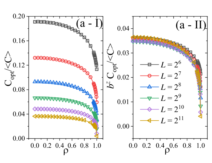
Figure 9: (a) I: Performance of the 2-opt-SAGCS as function of $\rho$ for different number of cities. (a) II: An approximate scaling for the plot is obtained with $z\approx-0.480$. (b): Analysis for different distributions of the points: Gaussian and uniform. The case (b) I corresponds to SS-SAGCS and the (b) II corresponds to 2-opt-SAGCS.

In this algorithm the walk start from an initial node and jumps to the nearest neighbor that has not yet been visited in the walk. The procedure is repeated until returning to the initial node by closing the cycle (Hamiltonian cycle). In this case, we applied this algorithm for $\rho=0$ and one finds a better approximation $\overline{C}_{opt}^{(NN)}(N=2048)=81.84\pm 0.34$ which leads to $\overline{C}_{opt}^{(NN)}/\overline{\left\langle C\right\rangle}_{\rho=0}\approx\allowbreak 0.0384$ which is much better than $C_{opt}^{(SS)}/\overline{\left\langle C\right\rangle}_{\rho=0}\approx 0.479$ which uses SS-SAGCS. Surprisingly, the 2-opt-SAGCS $C_{opt}^{(2-Opt)}=77.94(3)$, which leads to $\overline{C}_{opt}^{(2-Opt)}/\overline{\left\langle C\right\rangle}_{\rho=0}\approx 0.036\,$ which is even better than the NN algorithm.

There exist many specially arranged city distributions which make the NN algorithm gives the worst route. Here we are observing, it is an excellent heuristic, however, the 2-opt-SAGCS is still a better benchmark (almost a technical draw between the two heuristics) and the SAGCS has a good complexity when compared with NN algorithm. The SA has a complexity that can be writte in a general form as $O(c(N)\cdot N_{total})$ where $c(N)=O(1)$ for SS-SAGCS and $c(N)=O(N/2)$ at the worst case for the 2-opt-SAGCS. On the other hand the NN algorithm has a complexity $O(N^{2})$. Now it is interesting to consider some points: $N_{total}$ is not exactly related to $N$, since SA is a heuristic. Sure, $N_{steps}=\left\lfloor\frac{\ln(T_{\min}/T_{0})}{\ln\alpha}\right\rfloor$, and therefore it is a constant and does not depend on $N$. However, for larger values of $N$, it is needed to make considerations about $N_{iter}$. It is natural to expect that the larger $N$, larger the number of iterations of the internal loop and we should consider $N_{iter}=O(N)$ and the complexity of SA would be, at the worst case, a complexity $O(N^{2})$ which is exactly the complexity of NN-algorithm considering the analysis of a single starting point. It is important to mention that if we include the dependence on the initial point, since different initial points can lead to different optimal costs, the complexity of the NN-algorithm would then be $O(N^{3})$.

SA has modest optimal costs only when one uses a simple swap scheme, which is a naive technique when compared with 2-opt that can applied in general scenarios. In realistic situations, a generalization of the TSP, the VRP (vehicle routing problem) is the best alternative compared to the NN algorithm, and Tabu search algorithm as suggested by the authors in [20].

But again, our proposal in this paper is to analyze possible effects of the environment on the SA and not a detailed comparison among the methods, yet we could not miss to show the 2-opt-SAGCS in comparison to SS-SAGCS and the NN algorithm.

Thus, it is interesting to similarly analyze the size effects on the 2-opt-SAGCS exactly as we performed in plot in Fig. 8 (b).

Fig. 9 (a) I shows a similar decay of $C_{opt}/\left\langle C\right\rangle$ as function of $\rho$ but with values extremely lower than those of SS-SAGCS. Following what we applied to the SS-SAGCS, we performed a similar scaling for the 2-opt-SAGCS (Fig. 9 (a) II) but not so with the same quality. In this case the value is $z\approx-0.480$ which is very different than $z\approx 0.075$ found to SS-SAGCS.

It is also interesting to analyze the effects on the points considering different statistical distributions for the coordinates. Thus we prepared some experiments to capture the effects on the ratio $C_{opt}/\left\langle C\right\rangle$ as function of $\rho$ considering different distributions for the coordinates and the result is also surprising as Fig. 9 (b) shows. If before, we were considering $z_{1}$ and $z_{2}$ identically distributed uniform random variables, now we also consider them as Gaussian random variables for a comparison. It is important to mention that the $x$ and $y$ coordinates, have, the same average (zero) and variance of the variables $z_{1}$ and $z_{2}$ independently on $\rho$. As we previously reported, the effects to be observed depends strictly on $\rho$ since the average and variance do not change.

We can observe that in both cases, SS-SAGCS and 2-opt-SAGCS, respectively described by Fig. 9 (b-I) and Fig. 9 (b-II), the shape of the distribution seems to be more important than the variance once the Gaussian and the uniform random variables, with the same or different variances, lead to different curves, but gaussians with different variances produce practically the same behavior.

Finally, we also use an scaled cost:

$$C_{s}=\frac{C}{\sqrt{(x_{\max}-x_{\min})(y_{\max}-y_{\min})}}\text{,}$$ (15)

where $x(y)_{\max(\min)}=\max(\min)\{x(y)_{1},x(y)_{2},...,x(y)_{N}\}$, once, differently from uniform distribution, the Gaussian distribution is not supported on a finite interval. However, as the same Figs. 9 (b-I) and (b-II) show, no changes were observed in the two versions of the simulated annealing (the blue triangles correspond to Gaussian distribution with scaled cost).

For SS-SAGCS the lower the $N$, the better the performance, on the other hand, for the 2-opt-SAGCS, the higher the $N$, the better the performance as also can be observed in the Figs. 8 (b-I) and 9 (b-I).

4.2 Finding good fits for $\overline{C}_{opt}/\overline{\left\langle C\right\rangle}$ as a function of $\rho$

We also focus our results in finding good fits for $\overline{C}_{opt}/\overline{\left\langle C\right\rangle}$ as function of $\rho$. So follow a (heuristic and qualitative) method to find suitable fits for such behavior.

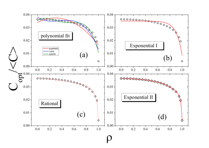
Figure 10: Fits for performance versus $\rho$ for SS-SAGCS and 2-opt-SAGCS. (a) preliminary polynomial fit (b) simple exponential (c) a reasonable fit with rational function (d) the best fit obtained by combining two exponentials.

First, we try a polynomial fit

$$p(\rho)=\sum_{i=0}^{n}a_{i}\rho^{i}$$

by testing $n=2$, $3$ and $4$ (with 3, 4, and 5 parameters respectively). The idea here is only to make a preliminary investigation. After that, we test exponential decay fits with only two parameters:

$$e_{I}(\rho)=e_{I}(0)+a_{1}e^{-\rho/\rho_{1}}$$

once that $e_{I}(0)$ is fixed and taken as $\overline{C}_{opt}/\overline{\left\langle C\right\rangle}(0)$ (it was visually investigated). Following, one considers a simple linear combination of exponential decays (with four parameters):

$$e_{II}(\rho)=e_{II}(0)+a_{1}e^{-\rho/\rho_{1}}+a_{2}e^{-\rho/\rho_{2}}\text{,}$$ (16)

also assuming empirically that $e_{II}(0)=\overline{C}_{opt}/\overline{\left\langle C\right\rangle}(0)$.

Alternatively, we also experimented other functions with four parameters, and the one that presented a good result was the rational function:

$$r(\rho)=\frac{a+b\rho}{1+c\rho+d\rho^{2}}\text{.}$$

This is shown in Fig. 10, which shows the different fits. The fits obtained in the different cases are summarized in table 2.

We can observe that the larger the degree of the polynomial fitted, the better the coefficient of determination $\alpha$ (the closer to one, the better it is). Our analysis also shows that in both cases, a single exponential (exponential I) is not enough to nicely fit the curve but with two exponential (four parameters), an excellent fit with $\alpha\approx 0.999$ can be obtained. With the same four parameters, the rational function gives a good result despite not so good as the linear combination of exponentials. It is important to mention that the coefficient $a$ found is exactly $\overline{C}_{opt}/\overline{\left\langle C\right\rangle}(0)$ in both cases (SS and 2opt-SAGCS) and the fit should be performed with three parameters. After all, one can observe that a better match is obtained by considering of a linear combination of the exponentials described by the Eq. 16. It seems to be a universal fit for $\overline{C}_{opt}/\overline{\left\langle C\right\rangle}$ $\times\rho$ for different values of $\rho$ for both SS-SAGCS and 2-opt-SAGCS.

SA	Quadratic	Cubic	Quartic
	$a_{0}=0.4710(42)$	$a_{0}=0.4815(34)$	$a_{0}=0.4755(26)$
	$a_{1}=0.067(19)$	$a_{1}=-0.076(30)$	$a_{1}=0.077(38)$
SS	$a_{2}=-0.132(18)$	$a_{2}=0.230(70)$	$a_{2}=-0.49(16)$
	$\alpha=0.92124$	$a_{3}=-0.237(45)$	$a_{3}=0.90(24)$
		$\alpha=0.96729$	$a_{4}=-0.57(12)$
			$\alpha=0.98495$
	$a_{0}=0.0339(21)$	$a_{0}=0.0382(21)$	$a_{0}=0.0353(20)$
	$a_{1}=0.0247(96)$	$a_{1}=0.0330(19)$	$a_{1}=0.041(29)$
2–opt	$a_{2}=-0.0419(91)$	$a_{2}=0.104(43)$	$a_{2}=-0.25(12)$
	$\alpha=0.78373$	$a_{3}=-0.096(28)$	$a_{3}=-0.46(19)$
		$\alpha=0.86162$	$a_{4}=-0.275(92)$
			$\alpha=0.90423$

SA	Exponential I	Rational	Exponential II
	$c_{1}=-3.1(1.2)\cdot 10^{-4}$	$a=0.47951(65)$	$c_{1}=-0.00190(13)$
	$\rho_{1}=0.179(13)$	$b=-0.4443(29)$	$\rho_{1}=-0.2852(62)$
SS	$\alpha=0.98309$	$c=-0.8923(39)$	$c_{2}=-(2.4\pm 3.3)\cdot 10^{-15}$
		$d=-0.0165(51)$	$\rho_{2}=-0.0331(15)$
		$\alpha=0.99798$	$\alpha=0.99984$
	$c_{1}=-4.9(7.9)\cdot 10^{-7}$	$a=0.03733(34)$	$c_{1}=-1.5(5.4)\cdot 10^{-26}$
	$\rho_{1}=-0.092(14)$	$b=-0.03719(35)$	$\rho_{1}=-0.0180(12)$
2–opt	$\alpha=0.93539$	$c=-0.832(24)$	$c_{2}=-3.27(61)\cdot 10^{-4}$
		$d=-0.136(25)$	$\rho_{2}=-0.261(14)$
		$\alpha=0.99312$	$\alpha=0.99914$

Table 2: Values of coefficients found after nonlinear fitting by using Levenberg-Marquadt method. The parameter $\alpha$ corresponds to coefficient of determination of each fit

4.3 Long tail effects

Finally, it is important to analyze the effects of long tailed distributions for the coordinates of the points distributed on the environment. In this case, we concentrate our analysis on $\rho=0$. Firstly, one chooses the variables $x$ and $y$ according to equations 11 and 12 for the SS-SAGCS. Plotting $C_{opt}/\left\langle C\right\rangle$ as function of $\gamma$ according to Fig. 11 (a) and (b).

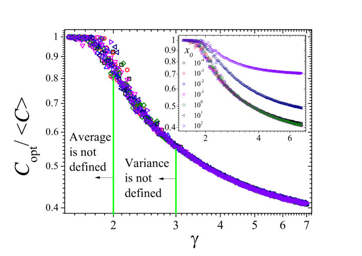
Figure 11: (a) $C_{opt}/\left\langle C\right\rangle$ as function of $\gamma$ for different values of $\varepsilon$ for the SS-SAGCS. We perform the scaling $C_{s}=C/\sqrt{(x_{\max}-x_{\min})(y_{\max}-y_{\min})}$. The inset plot shows the same curves without scaling. (b) Refinement of the region presenting the error bars. We can observe that $\gamma\approx 3.4$ corresponds to Gaussian distribution and $\gamma\approx 4.3$ corresponds to uniform distribution.

As expected $C_{opt}/\left\langle C\right\rangle$ decreases as function of exponent $\gamma$. Fig. 11 (a) shows this behavior for different values of $x_{0}$ considering the scaling in Eq. 15. We can observe a collapse of all curves independently on $x_{0}$. The inset plot shows the same plot without performing the scaling. It is interesting to notice the instability in the regions without defined variance $2\leq\gamma\leq 3$ but yet with some efficiency. For $\gamma<2$, which corresponds the region where the average cannot be defined, the SA has no efficiency which suggests that the algorithm should not be applied in these situations since $C_{opt}/\left\langle C\right\rangle\approx 1$. Fig. 11 (b) is only a refinement of one case in Fig. 11 (a) with uncertainty bars and also showing the values obtained with Gaussian and uniform distributions for a comparison (dashed blue lines).

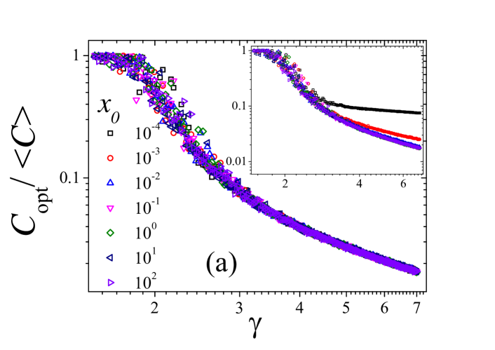
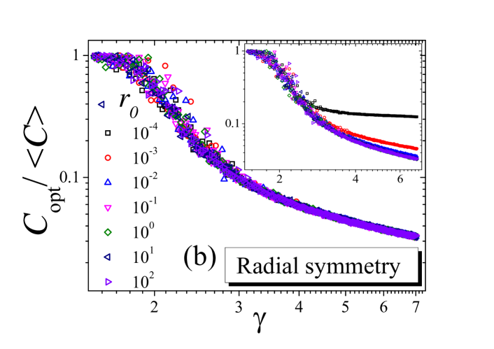
Figure 12: (a) $C_{opt}/\left\langle C\right\rangle$ as function of $\gamma$ for different values of $\varepsilon$ for 2-opt-SAGCS. We perform the scaling $C_{s}=C/\sqrt{(x_{\max}-x_{\min})(y_{\max}-y_{\min})}$. The inset plot shows the same curves without scaling. (b) The same plot by using power law coordinates with radial symmetry (Eq. 13).

Performing similar simulations to the plot of the Fig. 11 (a) but for the case 2opt-SAGCS, which can be observed in Fig. 12 (a) and the same conclusions can be drawn for $\gamma<2$ – the SA has no efficiency. In this case, SS-SAGCS and 2-opt-SAGCS are obviously equivalent since the scenario is really complicate. In Fig. 12 (b) we show the case where we used power-law coordinates with radial symmetry (Eq. 13). Surprisingly, the results do not change, showing that, independently from power law coordinates, the phenomena of the performance of the SA is universal as function of $\gamma$.

5 Summary and Conclusions

In this paper, we study the effects of the statistics on the coordinates of the points when we apply an standard simulated annealing algorithm to the travelling salesman problem. Our results are concerned with the long tail effects on the coordinates but also the correlation effects between these coordinates.

Our study shows that the performance of the simulated annealing increases as the correlation increases in both versions of the SA. The main reason is the dimensionality reduction, which transforms the simulated annealing at limit in an approximated sorting algorithm. The correlation effects show that the shape of distribution attributed to coordinates is more important than the variance when we compare Gaussian and uniform distributions.

Our results also suggest that the higher the exponent of the power law, the lower the simulated annealing performance, and for $\gamma<2$, i.e., distributions without the first moment, we have no performance of the SA, i.e., $C_{opt}/\left\langle C\right\rangle\approx 1$ even when one considers the benchmark for the SA, i.e., when the new configurations are obtained with 2-opt.

We obtained an universal behavior of $C_{opt}/\left\langle C\right\rangle$ $\times\rho$ and $C_{opt}/\left\langle C\right\rangle$ $\times\gamma$ never explored in the optimization problems with SA. In addition, we also show that 2-opt-SAGCS presents a better performance as larger is the system, differently from its inefficient version, the SS-SAGCS, where the reverse situation occurs.

We believe that both (correlation and long range effects) studies can bring an interesting knowledge for more technical applications in artificial intelligence, machine learning, and other areas. In special, in the search for global minimum in neural networks algorithms, maybe reviving the interests in simulating annealing as a viable alternative to stochastic gradient descent at the optimization step.

Appendix: Average distance between two points uniformly distributed in a square

Our original problem considers points uniformly distributed in the square such that $x\in[-1,1]$, $y\in[-1,1]$, i.e., an square of side 2. This is similar to consider points in the square defined by $x\in[0,2]$, $y\in[0,2]$, and thus the average distance between the points can be calculated by:

$$\begin{array}[]{lll}\left\langle d\right\rangle&=&\frac{1}{2^{4}}\int_{0}^{2}\int_{0}^{2}\int_{0}^{2}\int_{0}^{2}\sqrt{(x_{i}-x_{j})^{2}+(y_{i}-y_{j})^{2}}dx_{i}dx_{j}dy_{i}dy_{j}\\ &&\\ &=&\frac{1}{2^{3}}\int_{0}^{2}\int_{0}^{2}\int_{0}^{2}\int_{0}^{2}\sqrt{(\frac{x_{i}-x_{j}}{2})^{2}+(\frac{y_{i}-y_{j}}{2})^{2}}dx_{i}dx_{j}dy_{i}dy_{j}\end{array}$$

Performing the change of variables $z_{1}=\frac{x_{i}}{2}$, $z_{2}=\frac{x_{j}}{2}$, $z_{3}=\frac{y_{i}}{2}$, and $z_{4}=\frac{y_{i}}{2}$ ,and thus

$$\left\langle d\right\rangle=2\int_{0}^{1}\int_{0}^{1}\int_{0}^{1}\int_{0}^{1}\sqrt{(z_{1}-z_{2})^{2}+(z_{3}-z_{4})^{2}}dz_{1}dz_{2}dz_{3}dz_{4}$$

If $z_{1}$ and $z_{2}$ are uniformly distributed, so the random variable $u=\left|z_{1}-z_{2}\right|$ has a triangular distribution and the probability density function $2(1-u)$, and thus making the change of variables $u=\left|z_{1}-z_{2}\right|$, $v=\left|z_{3}-z_{4}\right|$, $w=z_{2}$, and $t=z_{3}$, one obtains:

$$\left\langle d\right\rangle=8\int_{0}^{1}\int_{0}^{1}(1-u)(1-v)\sqrt{u^{2}+v^{2}}dudv$$

Now is almost done! Making $u=r\cos\theta$ and $v=r\sin\theta$. However a trick is to perform the integration for the lower triangle where $0\leq\theta\leq\pi/4$

$$\begin{array}[]{lll}\left\langle d\right\rangle&=&16\int_{0}^{\pi/4}\int_{0}^{1/\sin\theta}(1-r\cos\theta)(1-r\sin\theta)r^{2}drd\theta\\ &&\\ &=&16\int_{0}^{\pi/4}\int_{0}^{1/\cos\theta}\left(r^{2}-r^{3}\left(\sin\theta+\cos\theta\right)+r^{4}\cos\theta\sin\theta\right)drd\theta\\ &&\\ &=&16\left[\frac{1}{3}\int_{0}^{\pi/4}\frac{1}{\cos^{3}\theta}d\theta-\frac{1}{4}\int_{0}^{\pi/4}\frac{\left(\sin\theta+\cos\theta\right)}{\cos^{4}\theta}d\theta+\frac{1}{5}\int_{0}^{\pi/4}\frac{\cos\theta\sin\theta}{\cos^{5}\theta}d\theta\right]\\ &&\\ &=&16\left[\frac{1}{12}\int_{0}^{\pi/4}\frac{1}{\cos^{3}\theta}d\theta-\frac{1}{20}\int_{0}^{\pi/4}\frac{\sin\theta}{\cos^{4}\theta}d\theta\right]\end{array}$$

And finally by performing these integrals one obtains

$$\left\langle d\right\rangle=\frac{1}{15}(4+2\sqrt{2}+10\ln(\sqrt{2}+1))$$

References

- [1] D. Sherrington, S. Kirkpatrick, Phys. Rev. Lett. 35, 1792 (1975)
- [2] S. Kirkpatrick , C. D. Gelatt Jr, M. P. Vecchi, Science 220, 671–677 (1983)
- [3] N. Metropolis, A. Rosenbluth, M. Rosenbluth, A. Teller, E. Teller, J. Chem. Phys. 21, 1087 (1953).
- [4] Christos Papadimitriou, Computational Complexity, Pearson (1993)
- [5] U.H.E. Hansmann, Y. Okamoto, Braz. J. Phys. 29, 187 (1999)
- [6] F. Mauger, C. Chandre, T. Uzer, Commun. Nonlinear Sci. Numer. Simul. 16, 2845 (2011)
- [7] S. Geman, D. Geman, IEEE Transactions on Pattern Analysis and Machine Learning 6, 721 (1984)
- [8] Y. Nourani, B. Andresen, J. Phys. A 31, 8373–8385 (1998)
- [9] P. J. M. van Laarhoven, E. H. L. Aarts, Simulated Annealing: Theory and Applications, Springer (1987)
- [10] S. Lin, B. W. Kernighan, Operations Research 21, 498-516 (1973)
- [11] S. Kirkpatrick, J. Stat. Phys. 34 975-986 (1984)
- [12] E. Aarts, J. Korst, Simulated Annealing and Boltzmann Machines, A Stochastic Approach to Combinatorial Optimization and Neural Computing, John Wiley & Sons (1989)
- [13] Simulated Annealing: Parallelization Techniques, Edited by R. Azencott, John Wiley & Sons (1992)
- [14] H. Szu, R. Hartley, Phys. Lett. A 122, 157-162 (1987)
- [15] L. Ingber, Mathl. Comput. Modelling 18, 29-57 (1993)
- [16] R. da Silva, S. D. Prado, Phys. Lett. A, (2020)
- [17] G. Gutin, A. Yeob, A. Zverovicha, Discrete Applied Mathematics 117, 81-86 (2002)
- [18] G. F. Lima, A. S. Martinez, and O. Kinouchi, Phys. Rev Lett. 87, 010603 (2001).
- [19] H. Eugene Stanley, Sergey V. Buldyrev, Nature 413 , 373–374 (2001)
- [20] P. Adi Wicaksono, D. Puspitasari, S. Ariyandanu, R. Hidayanti, IOP Conf. Ser.: Earth Environ. Sci. 426 012138 (2020)