Behavior of linear $L^{2}$-boosting algorithms in the vanishing learning rate asymptotic

Abstract

We investigate the asymptotic behaviour of gradient boosting algorithms when the learning rate converges to zero and the number of iterations is rescaled accordingly. We mostly consider $L^{2}$-boosting for regression with linear base learner as studied in Bühlmann and Yu, (2003) and analyze also a stochastic version of the model where subsampling is used at each step (Friedman,, 2002). We prove a deterministic limit in the vanishing learning rate asymptotic and characterize the limit as the unique solution of a linear differential equation in an infinite dimensional function space. Besides, the training and test error of the limiting procedure are thoroughly analyzed. We finally illustrate and discuss our result on a simple numerical experiment where the linear $L^{2}$-boosting operator is interpreted as a smoothed projection and time is related to its number of degrees of freedom.

Keywords: boosting, non parametric regression, statistical learning, stochastic algorithm, Markov chain, convergence of stochastic process.
Mathematics subject classification: 62G08, 60J20.

1 Introduction

In the past decades, boosting has become a major and powerful prediction method in machine learning. The success of the classification algorithm AdaBoost by Freund and Schapire, (1999) demonstrated the possibility to combine many weak learners in a sequential way in order to produce better predictions, with widespread applications in gene expression (Dudoit et al.,, 2002) or music genre identification (Bergstra et al.,, 2006), to name only a few. Friedman et al., (2000) were able to see a wider statistical framework that lead to the gradient boosting (Friedman,, 2001), where a weak learner (e.g., regression trees) is used to optimize a loss function in a sequential procedure akin to gradient descent. Choosing the loss function according to the statistical problem at hand results in a versatile and efficient tool that can handle classification, regression, quantile regression or survival analysis… The popularity of gradient boosting is also due to its efficient implementation in the R package gbm by Ridgeway, (2007).

Along the methodological developments, strong theoretical results have justified the good performance of boosting. Consistency of boosting algorithm, i.e. their ability to achieve the optimal Bayes error rate for large samples, is considered in Breiman, (2004), Zhang and Yu, (2005) or Bartlett and Traskin, (2007). The present paper is strongly influenced by Bühlmann and Yu, (2003) that proposes an analysis of regression boosting algorithms built on linear base learners thanks to explicit formulas for the boosted predictor and its error rate.

In this paper, we focus on gradient boosting for regression with square loss and we briefly describe the corresponding algorithm. Consider a regression model

$$Y=f(X)+\varepsilon$$ (1)

where the response $Y$ is real-valued, the predictor $X$ takes values in $[0,1]^{p}$, the regression function $f:[0,1]^{p}\to\mathbb{R}$ is measurable and the error $\varepsilon$ is centered, square integrable and independent of $X$. Based on a sample $(Y_{i},X_{i})_{1\leq i\leq n}$ of independent observations of the regression model (1), we aim at estimating the regression function $f$. Given a weak learner $L(x)=L(x;(Y_{i},X_{i})_{1\leq i\leq n})$, the boosting algorithm with learning rate $\lambda\in(0,1)$ produces a sequence of models $\hat{F}_{m}^{\lambda}(x)$, $m\geq 0$, by recursively fitting the weak learner to the current residuals and updating the model with a shrunken version of the fitted model. More formally, we define

$$\left\{\begin{array}[]{ll}\hat{F}_{0}^{\lambda}(x)&=\bar{Y}_{n},\\ \hat{F}_{m+1}^{\lambda}(x)&=\hat{F}_{m}^{\lambda}(x)+\lambda L(x;(R_{m,i}^{\lambda},X_{i})_{1\leq i\leq n}),\quad m\geq 0,\end{array}\right.$$ (2)

where $\bar{Y}_{n}$ denotes the empirical mean of $(Y_{i})_{1\leq i\leq n}$ and $(R_{m,i}^{\lambda})_{1\leq i\leq n}$ the residuals

$$R_{m,i}^{\lambda}=Y_{i}-\hat{F}_{m}^{\lambda}(X_{i}),\quad 1\leq i\leq n.$$

In practice, the shrinkage parameter $\lambda$ and the number of iterations $m$ are the main parameters and must be chosen suitably to achieve good performance. Common practice is to fix $\lambda$ to a small value, typically $\lambda=0.01$ or $0.001$, and then to select $m$ by cross-validation. Citing Ridgeway, (2007), with slight modifications to match our notations:

"The issues that most new users of gbm struggle with are the choice of tree numbers $m$ and shrinkage $\lambda$. It is important to know that smaller values of $\lambda$ (almost) always give improved predictive performance. That is, setting $\lambda=0.001$ will almost certainly result in a model with better out-of-sample predictive performance than setting $\lambda=0.01$. However, there are computational costs, both storage and CPU time, associated with setting shrinkage to be low. The model with $\lambda=0.001$ will likely require ten times as many iterations as the model with $\lambda=0.01$, increasing storage and computation time by a factor of $10$."

This citation clearly emphasizes the role of small learning rates in boosting. The purpose of the present paper is to prove the existence of a vanishing learning rate limit ($\lambda\to 0$) for the boosting algorithm when the number of iterations is rescaled accordingly. To our best knowledge, this is the first result in this direction. More precisely, in the case when the base learner is linear, we prove the existence of the limit

$$\hat{F}_{t}(x)=\lim_{\lambda\downarrow 0}\hat{F}_{[t/\lambda]}^{\lambda}(x),\quad t\geq 0.$$ (3)

We furthermore characterize the limit as the solution of a linear differential equation in infinite dimensional space and also analyse the corresponding training and test errors. The case of stochastic gradient boosting (Friedman,, 2002), where subsampling is introduced at each iteration, is also analysed: we prove the existence of a deterministic vanishing learning rate limit that corresponds to a modified deterministic base learner defined in a natural way. The analysis of this stochastic framework requires involved tools of Markov chain theory and the characterization of their convergence through generators (Ethier and Kurtz,, 1986; Stroock and Varadhan,, 2006). A limitation of our work is the strong assumption of linearity of the base learner: the ubiquitous regression tree does not satisfy this assumption and further work is needed to deal with this important case. Our results are of probabilistic nature: we focus on the existence and properties of the limit (3) for fixed sample size $n\geq 1$, while statistical issues such as consistency as $n\to\infty$ is left aside for further research.

The paper is structured as follows. In Section 2, we prove the existence of the vanishing learning rate limit (3) for the boosting procedure with linear base learner (Proposition 2.5), we characterize the limit as the solution of a linear differential equation in a function space (Theorem 2.7) and we analyze the training and test errors (Propositions 2.12 and 2.13). The stochastic gradient boosting where subsampling is introduced at each step is considered in Section 3. We prove that the vanishing learning rate limit still exists and that the convergence holds in quadratic mean (Corollary 3.5) and also in the sense of functional weak convergence in Skorokhod space (Theorem 3.6). A simple numerical experiment is presented in Section 4 in order to illustrate our theoretical findings, leading us to the interpretation of linear $L^{2}$-boosting as a smoothed projection where time is related to the degrees of freedom of the linear boosting operator. All the technical proofs are gathered in Section 5.

2 $L^{2}$-boosting with linear base learner

2.1 Framework

We consider the framework of boosting for regression with $L^{2}$-loss and linear base learner provided by Bühlmann and Yu, (2003). This framework allows for explicit computations relying on linear algebra. The regression design is assumed deterministic, or equivalently, we formulate our results conditionally on the predictor values $X_{i}=x_{i}$, $i=1,\ldots,n$. The space of measurable and bounded functions on $[0,1]^{p}$ is denoted by $L^{\infty}=L^{\infty}([0,1]^{p},\mathbb{R})$. Our main hypothesis is the following linearity assumption of the base learner $L$.

Assumption 2.1.

We assume that the base learner of the boosting algorithm (2) satisfies

$$L(x;(x_{i},Y_{i})_{1\leq i\leq n})=\sum_{j=1}^{n}Y_{j}g_{j}(x),\quad x\in[0,1]^{p},$$ (4)

where $g_{1},\ldots,g_{n}\in L^{\infty}$ may depend on $(x_{i})_{1\leq i\leq n}$.

It follows from Assumption 2.1 that $g_{j}$ is the output of the base learner for input $(Y_{i})_{1\leq i\leq n}=(\delta_{ij})_{1\leq i\leq n}$, where the Kroenecker symbol $\delta_{ij}$ is equal to $1$ if $i=j$ and $0$ otherwise.

Under Assumption 2.1, the boosting algorithm with input $(Y_{i},x_{i})_{1\leq i\leq n}$ and learning rate $\lambda\in(0,1)$ outputs a sequence of bounded functions $(\hat{F}_{m}^{\lambda})_{m\geq 1}$. The sequence remains in the finite dimensional linear space spanned in $L^{\infty}$ by the functions $g_{1},\ldots,g_{n}$ and the constant functions (due to the initialization equal to the constant function $\bar{Y}_{n}$). A straightforward recursion based on Equation (2) yields

$$\hat{F}_{m}^{\lambda}(x)=\bar{Y}_{n}+\sum_{i=1}^{n}w_{m,i}^{\lambda}g_{i}(x)$$ (5)

where the weights $w_{m}^{\lambda}=(w_{m,i}^{\lambda})_{1\leq i\leq n}$ satisfy

$$\left\{\begin{array}[]{ll}w_{0,i}^{\lambda}&\equiv 0\\ w_{m+1,i}^{\lambda}&=w_{m,i}^{\lambda}+\lambda(Y_{i}-\bar{Y}_{n})-\lambda\sum_{j=1}^{n}w_{m,j}^{\lambda}g_{j}(x_{i})\end{array}\right..$$

This linear recursion system can be rewritten in vector form as

$$\left\{\begin{array}[]{ll}w_{0}^{\lambda}&\equiv 0\\ w_{m+1}^{\lambda}&=(I-\lambda S)w_{m}^{\lambda}+\lambda\tilde{Y}\end{array}\right.,$$ (6)

with $S=(g_{j}(x_{i}))_{1\leq i,j\leq n}$, $\tilde{Y}=(Y_{i}-\bar{Y}_{n})_{1\leq i\leq n}$ the centered observations and $I$ the $n\times n$ identity matrix. This linear recursion is easily solved, yielding the following proposition.

Proposition 2.2.

Under Assumption 2.1, the boosting algorithm output $\hat{F}_{m}^{\lambda}$ is given by Equation (5) with weights

$$w_{m}^{\lambda}=\lambda\sum_{j=0}^{m-1}(I-\lambda S)^{j}\tilde{Y},\quad m\geq 0.$$ (7)

If the matrix $S$ is invertible, then

$$w_{m}^{\lambda}=S^{-1}\left[I-(I-\lambda S)^{m}\right]\tilde{Y},\quad m\geq 0.$$

Note that this result is similar to Proposition 1 in Bühlmann and Yu, (2003), but they consider only the values on the observed sample $(x_{i})_{1\leq i\leq n}$ while we provide the extrapolation to $x\in[0,1]^{p}$ more explicitly. Also we consider a different initialization to the empirical mean instead of initialization to zero, which seems more relevant in practice.

Example 2.3.

A simple example satisfying Assumption 2.1 is the Nadaraya-Watson estimator (see Nadaraya, (1964) and Watson, (1964))

$$L(x)=\frac{\sum_{i=1}^{n}K_{h}(x-x_{i})Y_{i}}{\sum_{i=1}^{n}K_{h}(x-x_{i})},\quad x\in[0,1]^{p},$$

where $h>0$ is the bandwidth, $K:\mathbb{R}^{p}\to(0,+\infty)$ is the kernel, i.e. a density function, and $K_{h}(z)=h^{-d}K(z/h)$ the rescaled kernel.

Example 2.4.

A more involved example of base learner, discussed in Bühlmann and Yu, (2003) Section 3.2, is the smoothing spline in dimension $p=1$. For $r\geq 1$ and $\nu>0$, the smoothing spline $L$ is the unique minimizer over $\mathcal{W}_{2}^{(r)}$ of the penalized criterion

$$\sum_{i=1}^{n}(Y_{i}-L(x_{i}))^{2}+\nu\int_{0}^{1}(L^{(r)}(x))^{2}\mathrm{d}x,$$

where $\mathcal{W}_{2}^{(r)}$ denotes the Sobolev space of functions that are continuously differentiable of order $r-1$ with square integrable weak derivative of order $r$. Assuming $0<x_{1}<\cdots<x_{n}<1$, the solution is known to be piecewise polynomial function of degree $r+1$ with constant derivative of order $r+1$ on $n+1$ intervals $(0,x_{1}),\ldots,(x_{n},1)$. It is used in Bühlmann and Yu, (2003) that the matrix $S$ is symmetric definite positive with positive eigenvalues $1=\mu_{1}=\ldots=\mu_{r}>\ldots>\mu_{n}>0$, see Wahba, (1990).

2.2 The vanishing learning rate asymptotic

We next consider the existence of a limit in the vanishing learning rate asymptotic $\lambda\to 0$. The explicit simple formulas from Proposition 2.2 allows for a simple analysis. We recall that the exponential of a square matrix $M$ is defined by

$$\exp(M)=\sum_{k\geq 0}\frac{1}{k!}M^{k}.$$

Proposition 2.5.

Under Assumption 2.1, as $\lambda\to 0$, we have

$$\hat{F}_{[t/\lambda]}^{\lambda}(x)\longrightarrow\hat{F}_{t}(x),\quad t\geq 0,\ x\in[0,1]^{p},$$ (8)

uniformly on compact sets $[0,T]\times[0,1]^{p}$, $T>0$, where the limit satisfies

$$\hat{F}_{t}(x)=\bar{Y}_{n}+\sum_{i=1}^{n}w_{t,i}g_{i}(x)$$ (9)

with weights $w_{t}=(w_{t,i})_{1\leq i\leq n}$ given by

$$w_{t}=-\sum_{j\geq 1}\frac{(-t)^{j}}{j!}S^{j-1}\tilde{Y},\quad t\geq 0.$$ (10)

If the matrix $S$ is invertible, then

$$w_{t}=S^{-1}\left(I-e^{-tS}\right)\tilde{Y},\quad t\geq 0.$$ (11)

The formulas are even more explicit in the case when $S$ is a symmetric matrix because it can then be diagonalized in an orthonormal basis of eigenvectors.

Corollary 2.6.

Suppose Assumption 2.1 is satisfied and $S=(g_{j}(x_{i}))_{1\leq i,j\leq n}$ is a symmetric matrix. Denote by $(\mu_{j})_{1\leq j\leq n}$ the eigenvalues of $S$ and by $(u_{j})_{1\leq j\leq n}$ the corresponding eigenvectors. Then the vanishing learning rate asymptotic yields the weights

$$w_{t}=\sum_{j=1}^{n}\frac{1-e^{-\mu_{j}t}}{\mu_{j}}u_{j}u_{j}^{\mathrm{T}}\tilde{Y}$$

and the limit

$$\hat{F}_{t}(x)=\bar{Y}_{n}+\sum_{1\leq i,j\leq n}\frac{1-e^{-\mu_{j}t}}{\mu_{j}}\left(v_{i}^{\mathrm{T}}u_{j}u_{j}^{\mathrm{T}}\tilde{Y}\right)g_{i}(x),$$ (12)

with $(v_{i})_{1\leq i\leq n}$ the canonical basis in $\mathbb{R}^{n}$. When $\mu=0$, we use extension by continuity, that is the convention $(1-e^{-\mu t})/\mu=t$.

Interestingly, the limit function $(\hat{F}_{t})_{t\geq 0}$ appearing in the vanishing learning rate asymptotic can be characterized as the solution of a linear differential equation in infinite dimensional space. The intuition is quite clear from the following heuristic: the boosting dynamic

$$\hat{F}_{m+1}^{\lambda}=\hat{F}_{m}^{\lambda}+\lambda\sum_{i=1}^{n}(Y_{i}-\hat{F}_{m}^{\lambda}(x_{i}))g_{i}$$

implies, for $t=\lambda m$,

$$\lambda^{-1}\left(\hat{F}_{[(t+\lambda)/\lambda]}^{\lambda}-\hat{F}_{[t/\lambda]}^{\lambda}\right)=\sum_{i=1}^{n}(Y_{i}-\hat{F}_{[t/\lambda]}^{\lambda}(x_{i}))g_{i}.$$

Letting $\lambda\to 0$, the convergence $\hat{F}_{[t/\lambda]}^{\lambda}\to\hat{F}_{t}$ suggests

$$\hat{F}_{t}^{\prime}=\sum_{i=1}^{n}(Y_{i}-\hat{F}_{t}(x_{i}))g_{i}.$$

We make this heuristic rigorous in the following proposition. For $t\geq 0$, we consider $\hat{F}_{t}$ as an element of the Banach space $L^{\infty}=L^{\infty}([0,1]^{p},\mathbb{R})$ and prove that $(\hat{F}_{t})_{t\geq 0}$ is the unique solution of a linear differential equation. More precisely, it is easily seen that the linear operator $\mathcal{L}:L^{\infty}\to L^{\infty}$ defined by

$$\mathcal{L}(Z)=\sum_{i=1}^{n}Z(x_{i})g_{i},\quad Z\in L^{\infty},$$

is bounded and we consider the differential equation in the Banach space $L^{\infty}$

$$Z^{\prime}(t)=-\mathcal{L}(Z(t))+G,\quad t\geq 0,$$ (13)

with $G=\sum_{i=1}^{n}Y_{i}g_{i}$.

Theorem 2.7.

1. For all $Z_{0}\in L^{\infty}$, the differential equation (13) has a unique solution satisfying $Z(0)=Z_{0}$. Furthermore, if there exists $\mathcal{Y}\in L^{\infty}$ such that $\mathcal{L}(\mathcal{Y})=G$, this solution is explicitly given by

   $$Z(t)=(e^{-t\mathcal{L}})Z_{0}+(\mathrm{Id}-e^{-t\mathcal{L}})\mathcal{Y},\quad t\geq 0.$$ (14)

2. The function $(\hat{F}_{t})_{t\geq 0}$ is the solution of (13) with initial condition $\bar{Y}_{n}$. Assuming there exists $\mathcal{Y}\in L^{\infty}$ such that $\mathcal{L}(\mathcal{Y})=G$, we thus have

   $$\hat{F}_{t}=(e^{-t\mathcal{L}})\bar{Y}_{n}+(\mathrm{Id}-e^{-t\mathcal{L}})\mathcal{Y},\quad t\geq 0.$$

Remark 2.8.

The condition $\mathcal{L}(\mathcal{Y})=G$ is satisfied as soon as $\mathcal{Y}(x_{i})=Y_{i}$, $1\leq i\leq n$. In particular, it holds if the $x_{i}$’s are pairwise distinct. It is used mostly for convenience and elegance of notations. Indeed we have

$$(\mathrm{Id}-e^{-t\mathcal{L}})(\mathcal{Y})=-\sum_{k\geq 1}\frac{(-t)^{k}}{k!}\mathcal{L}^{k}(\mathcal{Y})=\sum_{k\geq 1}\frac{(-1)^{k-1}t^{k}}{k!}\mathcal{L}^{k-1}(G)$$

and, if the existence of $\mathcal{Y}$ is not granted, one can replace in formula (14) the term involving $\mathcal{Y}$ by the series in the right hand side of the previous equation and check that this provides a solution of (13) in the general case.

Finally, we discuss the notion of stability of the boosting procedure. It requires that the output of the boosting algorithm does not explodes for large time values.

Definition 2.9.

The boosting algorithm is called stable if, for all possible input $(Y_{i})_{1\leq i\leq n}$, the output $(\hat{F}_{t})_{t\geq 0}$ remains uniformly bounded as $t\to\infty$.

It is here convenient to assume the following:

Assumption 2.10.

In Equation (4), the functions $(g_{i})_{1\leq i\leq n}$ are linearly independent and such that $\sum_{i=1}^{n}g_{i}(x)\equiv 1$.

The linear independence is sensible if the points $(x_{i})_{1\leq i\leq n}$ are pairwise distinct. The constant sum implies that for constant input $Y_{i}=1$, $1\leq i\leq n$, the output $L(x)\equiv 1$ is also constant. Both are mild assumptions satisfied by most learners in practice.

The stability can be characterized in terms of the Jordan normal form of the matrix $S$, see for instance Horn and Johnson, (2013). We recall that the Jordan normal form of $S$ is a block diagonal matrix where each block, called Jordan block, is an upper triangular matrix of size $s\times s$ with a complex eigenvalue $\mu$ on the main diagonal and ones on the superdiagonal. The matrix can be diagonalized if and only if all its Jordan blocks have size $1$.

Proposition 2.11.

Suppose Assumptions 2.1 and 2.10 are satisfied. Then the boosting procedure algorithm is stable if and only if all the blocks of the Jordan normal form of $S$ satisfy:

• the eigenvalue has a positive real part;

• the eigenvalue has a null real part and the block has size $1$.

In particular, if $S$ is symmetric, the boosting procedure is stable if and only if all the eigenvalues of $S$ are non-negative.

2.3 Training and test error

We next consider the performance of the boosting regression algorithm in terms of $L^{2}$-loss, also known as mean squared error. We focus mostly on the vanishing learning rate asymptotic, although version of the results below could be derived for positive learning rate $\lambda$.

The training error is assessed on the training set used to fit the boosting predictor and compares the observations $Y_{i}$ to their predicted values $\hat{F}_{t}(X_{i})$, i.e.

$$\mathrm{err}_{train}(t)=\frac{1}{n}\sum_{i=1}^{n}(Y_{i}-\hat{F}_{t}(x_{i}))^{2}.$$ (15)

The generalization capacity of the algorithm is assessed on new observations that are not used during the fitting procedure. For test observations $(Y_{i}^{\prime},X_{i}^{\prime})_{1\leq i\leq n^{\prime}}$, independent of the training sample, the test error is defined by

$$\mathrm{err}_{test}(t)=\frac{1}{n^{\prime}}\sum_{i=1}^{n^{\prime}}(Y_{i}^{\prime}-\hat{F}_{t}(X_{i}^{\prime}))^{2}.$$ (16)

We also consider a simpler version of the test error where extrapolation in the feature space is not evaluated and we take $n^{\prime}=n$ and $X^{\prime}_{i}=x_{i}$. Then, the test error writes

$$\mathrm{err}_{test}(t)=\frac{1}{n}\sum_{i=1}^{n}(Y_{i}^{\prime}-\hat{F}_{t}(x_{i}))^{2},$$ (17)

and allows for simpler formulas with nice interpretation.

We first consider the behavior of the training error as defined in Equation (15). Note that

$$\mathrm{err}_{train}(t)=\frac{1}{n}\|R_{t}\|^{2}$$

where $R_{t}$ is the vector of residuals at time $t$ defined by

$$R_{t}=(Y_{i}-\hat{F}_{t}(x_{i}))_{1\leq i\leq n},\quad t\geq 0,$$

and $\|\cdot\|$ denotes the Euclidean norm on $\mathbb{R}^{n}$. Furthermore, Proposition 2.5 implies $R_{t}=e^{-tS}\tilde{Y}$, $t\geq 0$, so that

$$\mathrm{err}_{train}(t)=\frac{1}{n}\|e^{-tS}\tilde{Y}\|^{2},\quad t\geq 0.$$

The following proposition is related to Proposition 3 and Theorem 1 in Bühlmann and Yu, (2003).

Proposition 2.12.

Suppose Assumptions 2.1 and 2.10 are satisfied.

• We have $\lim_{t\to\infty}\mathrm{err}_{train}(t)=0$ for all possible input $(Y_{i})_{1\leq i\leq n}$ if and only if all the eigenvalues of $S$ have a positive real part.

• The training error satisfies

  $$\mathbb{E}[\mathrm{err}_{train}(t)] =\mathrm{bias}^{2}(t)+\mathrm{var}_{train}(t),$$ (18)

  $$\mathrm{bias}^{2}(t) =\frac{1}{n}\|e^{-tS}\tilde{f}\|^{2},$$

  $$\mathrm{var}_{train}(t) =\frac{\sigma^{2}}{n}\mathrm{Trace}\left(e^{-tS}Je^{-tS^{T}}\right),$$

  with $J=I-\frac{1}{n}1_{n}1_{n}^{T}$, $\tilde{f}=f-\bar{f}1_{n}$, $f=(f(x_{i}))_{1\leq i\leq n}$ and $\bar{f}=\frac{1}{n}\sum_{i=1}^{n}f(x_{i})$.

• If $S$ is symmetric with positive eigenvalues $(\mu_{i})_{1\leq i\leq n}$ and corresponding eigenvectors $(u_{i})_{1\leq i\leq n}$,

  $$\mathbb{E}[\mathrm{err}_{train}(t)]=\frac{1}{n}\sum_{i=1}^{n}(u_{i}^{T}\tilde{f})^{2}e^{-2t\mu_{i}}+\frac{\sigma^{2}}{n}\sum_{i=1}^{n}\|Ju_{i}\|^{2}e^{-2t\mu_{i}}.$$

  The expected training error is strictly decreasing and converges to $0$ exponentially fast as $t\to\infty$.

The convergence of the training error to zero implies that the boosting procedure is stable as considered in Proposition 2.11 but the converse is not true since some eigenvalues may have a real part equal to zero. When $S$ is symmetric definite positive, the expected training error converges exponentially fast to $0$ (this was already proved in Bühlmann and Yu, (2003) Theorem 1 for $\lambda>0$) but this exponential rate of convergence has to be taken with care since $S$ may have very small eigenvalues, see the numerical illustration in Section 4.

The fact that the residuals converge to zero suggests that the boosting procedure eventually overfits the training observations and loses generalization power. A simple analysis of this overfit is provided by the test error with fixed covariates $X_{i}^{\prime}=x_{i}$, as defined by Equation (17). For the sake of simplicity, we emphasize the case when $S$ is symmetric.

Proposition 2.13.

• The test error with fixed covariates defined by Equation (17) satisfies

  $$\mathbb{E}[{\mathrm{err}}_{test}(t)] =\mathrm{bias}^{2}(t)+\mathrm{var}_{test}(t),$$

  $$\mathrm{bias}^{2}(t) =\frac{1}{n}\|e^{-tS}\tilde{f}\|^{2},$$

  $$\mathrm{var}_{test}(t) =\frac{\sigma^{2}}{n}+\frac{\sigma^{2}}{n}\mathrm{Trace}\left((I-e^{-tS})J(I-e^{-tS})^{T}\right).$$

• If $S$ is symmetric with positive eigenvalues $(\mu_{i})_{1\leq i\leq n}$ and associated eigenvectors $(u_{i})_{1\leq i\leq n}$,

  $$\mathrm{bias}^{2}(t) =\frac{1}{n}\sum_{i=1}^{n}(u_{i}^{T}\tilde{f})^{2}e^{-2t\mu_{i}},$$

  $$\mathrm{var}_{test}(t) =\sigma^{2}+\frac{\sigma^{2}}{n}+\frac{\sigma^{2}}{n}\sum_{i=1}^{n}\|Ju_{i}\|^{2}(1-e^{-t\mu_{i}})^{2},$$

  so that the the following properties hold:

  • the squared bias is decreasing, convex and vanishes as $t\to\infty$;

  • the variance is increasing and with limit $2\sigma^{2}$ as $t\to\infty$;

  • the expected test error is decreasing in the neighborhood of zero, eventually increasing and with limit $2\sigma^{2}$ as $t\to\infty$.

We retrieve with explicit theoretical formulas the known behavior of boosting in practice: the choice of $t\geq 0$ is crucial in the bias/variance trade-off. Small values of $t\geq 0$ lead to underfitting while overfitting appears for larger time values. In the early stage of the procedure, the bias decreases more rapidly that the variance increases, leading to a reduced test error. In practice, cross-validation and early stopping is used to estimate the test error and choose when to stop the boosting procedure, see Zhang and Yu, (2005).

Remark 2.14.

When the boosting algorithm is initialized at $\hat{F}_{0}=0$ as in Bühlmann and Yu, (2003), the expected training and test error from Propositions 2.12 and 2.13 become

$$\mathbb{E}[\mathrm{err}_{train}(t)]=\frac{1}{n}\sum_{i=1}^{n}(u_{i}^{T}f)^{2}e^{-2t\mu_{i}}+\frac{\sigma^{2}}{n}\sum_{i=1}^{n}\|u_{i}\|^{2}e^{-2t\mu_{i}}$$

and

$$\mathbb{E}[\mathrm{err}_{test}(t)]=\frac{1}{n}\sum_{i=1}^{n}(u_{i}^{T}f)^{2}e^{-2t\mu_{i}}+\frac{\sigma^{2}}{n}+\frac{\sigma^{2}}{n}\sum_{i=1}^{n}\|u_{i}\|^{2}e^{-2t\mu_{i}}.$$

These values are always larger than those with initialization $\hat{F}_{0}=\bar{Y}_{n}$, whence we recommend initialization to the empirical mean.

When the test error includes extrapolation in the predictor space - i.e. the new test observations $(Y_{i}^{\prime},X_{i}^{\prime})_{1\leq i\leq n^{\prime}}$ are i.i.d. and independent of the training observation as in Equation (16) - the formula we obtain for its expectation is more difficult to analyse.

Proposition 2.15.

Assume $S$ is symmetric with positive eigenvalues. The test error defined by Equation (16) has expectation

$$\mathbb{E}[\mathrm{err}_{test}(t)] =\frac{n+1}{n}\sigma^{2}+\mathbb{E}\big{[}\big{(}f(X^{\prime})-\bar{f}-\tilde{f}^{T}S^{-1}\left(I-\mathrm{e}^{-tS}\right)g(X^{\prime})\big{)}^{2}\big{]}$$

$$\quad+\sigma^{2}\mathbb{E}\left[g(X^{\prime})^{T}\left(I-\mathrm{e}^{-tS}\right)S^{-1}JS^{-1}\left(I-\mathrm{e}^{-tS}\right)g(X^{\prime})\right]$$

with $g(X^{\prime})=(g_{i}(X^{\prime}))_{1\leq i\leq n}$.

3 Stochastic gradient boosting

Following Friedman, (2002), it is common practice to use a stochastic version of the boosting algorithm where subsampling is introduced at each step of the procedure. The package gbm by Ridgeway, (2007) uses the subsampling rate equal to $50\%$ by default, meaning that each step involves only a subsample with half of the observations randomly chosen. This subsampling is known to have a regularization effect and we consider in this section the existence of the vanishing learning rate limit for such stochastic boosting algorithms.

3.1 Framework

We consider the following stochastic boosting algorithm that encompasses stochastic gradient boosting, see Example 3.2 below. We assume the weak learner $L(x)=L(x;(x_{i},y_{i})_{1\leq i\leq n},\xi)$ depends on the observations $(x_{i},y_{i})_{1\leq i\leq n}$ and on an external source of randomness $\xi$ with a finite set $\Xi$ of possible values. We define the stochastic boosting algorithm by the recursion

$$\left\{\begin{array}[]{ll}\hat{F}_{0}^{\lambda}(x)&=\bar{Y}_{n},\\ \hat{F}_{m+1}^{\lambda}(x)&=\hat{F}_{m}^{\lambda}(x)+\lambda L(x;(R_{m,i}^{\lambda},X_{i})_{1\leq i\leq n},\xi_{m+1}),\quad m\geq 0,\end{array}\right.$$ (19)

where $\xi_{m}$, $m\geq 1$, are i.i.d. $\Xi$-valued random variables independent of $(X_{i},Y_{i})_{1\leq i\leq n}$ and $R_{m,i}^{\lambda}=Y_{i}-\hat{F}_{m}^{\lambda}(X_{i})$, $1\leq i\leq n$, are the residuals.

Assumption 3.1.

We assume that the base learner of the stochastic boosting algorithm (19) satisfies

$$L(x;(x_{i},Y_{i})_{1\leq i\leq n},\xi)=\sum_{j=1}^{n}Y_{j}g_{j}(x,\xi),\quad x\in[0,1]^{p},$$

where $g_{1},\ldots,g_{n}\in L^{\infty}$ may depend on $(x_{i})_{1\leq i\leq n}$ and $\xi\in\Xi$.

We assume that $\Xi$ is finite mostly for simplicity and also because it is enough to cover two particularly important cases.

Example 3.2.

Starting from a base learner $L$ satisfying Assumption 2.1 (with $n$ replaced by $[sn]$) and applying stochastic subsampling (Friedman,, 2002), we obtain a stochastic setting that satisfies Assumption 3.1. Let the sample size $n\geq 1$ be fixed and consider subsambling with rate $s\in(0,1)$, e.g. $s=50\%$. Define $\Xi$ as the set of all subsets $\xi$ of $\{1,\ldots,n\}$ with fixed size $[sn]$. Note that $\Xi$ is finite with cardinality $n\choose{[sn]}$. The learner $L$ fitted on subsample $\xi\in\Xi$ is written

$$L(x;(x_{i},Y_{i})_{1\leq i\leq n},\xi)=L(x;(x_{i},Y_{i})_{i\in\xi}).$$

We use here a mild abuse of notation: in the left hand side, $L$ denotes the randomized learner, the sample size is $n$ and subsampling is introduced by $\xi$; in the right hand side, $L$ denotes the deterministic base learner and the sample size is $[sn]$. Stochastic boosting corresponds to Algorithm (19) with the sequence $(\xi_{m})_{m\geq 1}$ uniformly distributed on $\Xi$, which corresponds to uniform subsampling.

Example 3.3.

Another important example covered by the stochastic boosting algorithm (19) is the design of additive models. The idea is to provide an approximation of the regression function $f(x)$, $x\in[0,1]^{p}$, by an additive model of the form $f_{1}(x^{(1)})+\cdots+f_{p}(x^{(p)})$, where $x^{(j)}$ denotes the $j$th component of $x$ and $f_{j}$ the principal effect of $x^{(j)}$. Such an additive model does not include interactions between different components. Assume that a base learner $L$ with one-dimensional covariate space $[0,1]$ is given and that $L$ satisfies Assumption 2.1 with $p=1$. For instance, $L$ can be a smoothing spline as in Example 2.4, see Bühlmann and Yu, (2003) Section 4. We consider stochastic regression boosting where the base learner $L$ is sequentially applied with a randomly chosen predictor. Formally, set

$$L(x;(x_{i},Y_{i})_{1\leq i\leq n},\xi)=L(x;(x_{i}^{(\xi)},Y_{i})_{1\leq i\leq n}),\quad\xi=1,\ldots,p.$$

It is easily checked that the learner in the left hand side satisfies Assumption 3.1 and that algorithm (19) with $(\xi_{m})_{m\geq 1}$ uniformly distributed on $\Xi=\{1,\ldots,p\}$ outputs a sequence of additive models. This strategy is often used with a more involved procedure where, at each step, the $p$ different possible predictors are considered and the best one is kept, see Bühlmann and Yu, (2003) Section 4. But this falls beyond Assumption 3.1 because choosing the optimal component is not a linear operation and the randomized choice proposed here is a sensible alternative satisfying Assumption 3.1.

3.2 Convergence of finite dimensional distributions

For fixed input $(Y_{i},x_{i})_{1\leq i\leq n}$, the stochastic boosting algorithm (19) provides a sequence of stochastic processes $\hat{F}_{m}^{\lambda}$, $m\geq 1$, and we consider the vanishing learning rate limit (3) under Assumption 3.1. We first prove convergence of the finite dimensional distributions thanks to elementary moment computations formulated in the next proposition. Expectation and variance are considered with respect to $(\xi_{m})_{m\geq 1}$ while the input $(x_{i},Y_{i})_{1\leq i\leq n}$ is considered fixed and we note $\mathbb{E}_{\xi}$ and $\mathrm{Var}_{\xi}$ to emphasize this. We define

$$\bar{g}_{j}(x)=\mathbb{E}_{\xi}[g_{j}(x,\xi)],\quad x\in[0,1]^{p},\ j=1,\ldots,n,$$

and

$$S=(\bar{g}_{i}(x_{j}))_{1\leq i,j\leq n}.$$ (20)

Note that $\bar{g}_{1},\ldots,\bar{g}_{n}$ are well-defined and in $L^{\infty}$ because $\Xi$ is finite so that there are no measurability or integrability issues.

Proposition 3.4.

Consider the boosting algorithm (19) under Assumption 3.1 and let the input $(Y_{i},x_{i})_{1\leq i\leq n}$ be fixed.

1. For $x\in[0,1]^{p}$ and $m\geq 0$,

   $$\mathbb{E}_{\xi}[\hat{F}_{m}^{\lambda}(x)]=\bar{Y}_{n}+\sum_{i=1}^{n}w_{m,i}^{\lambda}\bar{g}_{i}(x),$$ (21)

   where $w_{m}^{\lambda}=(w_{m,i}^{\lambda})_{1\leq i\leq n}$ is defined by (7) with $S$ given by (20).

2. There exists a positive constant $K$ such that, for all $x\in[0,1]^{p}$, $m\geq 0$ and $\lambda<1$,

   $$\mathrm{Var}_{\xi}[\hat{F}_{m}^{\lambda}(x)]\leq K(m+1)\lambda^{2}(1+K\lambda)^{m}n\|\tilde{Y}\|_{\infty}^{2}\left\{1+(\lambda mK)^{2}\mathrm{e}^{2\lambda m\|S\|_{\infty}}\right\},$$

   where $\|\cdot\|_{\infty}$ denotes here the maximum norm on $\mathbb{R}^{n}$. We use the same notation for the infinity-norm of $n\times n$ matrices.

As will be clear from the proof, the constant $K$ can be taken as $2M_{1}+M_{1}^{2}+(n+1)M_{2}$, where

$$M_{1}=\max_{1\leq j\leq n+1}\sum_{i=1}^{n}|\bar{g}_{i}(x_{j})|$$ (22)

and

$$M_{2}=\max_{1\leq j\leq n+1}\sum_{i=1}^{n}\mathrm{Var}_{\xi}[g_{i}(x_{j})].$$ (23)

Corollary 3.5.

For all $t\geq 0$ and $x\in[0,1]^{p}$, the convergence (3) holds in quadratic mean with deterministic limit

$$\hat{F}_{t}(x)=\bar{Y}_{n}+\sum_{i=1}^{n}w_{t,i}\bar{g}_{i}(x),$$ (24)

where $w_{t}=(w_{t,i})_{1\leq i\leq n}$ is defined by (10) with $S$ given by (20).

Corollary 3.5 states that the vanishing learning rate limit $\hat{F}_{t}(x)$ for the stochastic boosting algorithm (19) is exactly the same as the one for the deterministic boosting algorithm (2) with base learner

$$\bar{L}(x;(x_{i},Y_{i})_{1\leq i\leq n}) =\mathbb{E}_{\xi}[L(x;(x_{i},Y_{i})_{1\leq i\leq n},\xi)]$$

$$=\sum_{j=1}^{n}Y_{j}\bar{g}_{j}(x).$$

In particular, the properties of the limit process $(\hat{F}_{t})_{t\geq 0}$ have been studied in Section 2: characterization by a differential equation, behaviour of the training and test error, etc.

3.3 Weak convergence in function space

Corollary 3.5 implies that the convergence

$$\hat{F}_{[t/\lambda]}^{\lambda}(x)\longrightarrow\hat{F}_{t}(x),\quad\mbox{as $\lambda\to 0$},$$

holds in the sense of finite dimensional distributions, that is joint convergence in distribution of the values of the processes at finitely many points $(t_{i},x_{i})_{1\leq i\leq k}$. We strengthen here this convergence into a weak convergence of stochastic processes in the Skorokhod space $\mathbb{D}([0,\infty),L^{\infty})$ of càd-làg functions with values in $L^{\infty}$. We refer to Billingsley, (1999, Section 16) for background on the Skorokhod space $\mathbb{D}([0,\infty),\mathbb{R})$ and to Ethier and Kurtz, (1986, Section 3.5) for the general Skorokhod space $\mathbb{D}([0,\infty),E)$ on a metric space $E$.

Theorem 3.6.

Consider the boosting algorithm (19) under Assumption 3.1 and let the input $(Y_{i},x_{i})_{1\leq i\leq n}$ be fixed.

1. For fixed $\lambda>0$, the boosting sequence $(\hat{F}_{m}^{\lambda})_{m\geq 0}$ is a time homogeneous Markov chain with values in $L^{\infty}$.

2. As $\lambda\to 0$, the convergence in distribution

   $$(\hat{F}_{[t/\lambda]}^{\lambda})_{t\geq 0}\stackrel{{\scriptstyle d}}{{\longrightarrow}}(\hat{F}_{t})_{t\geq 0}$$ (25)

   holds in the Skorokhod space $\mathbb{D}([0,\infty),L^{\infty})$.

Our proof relies on the theory of approximations of Markov chains by diffusions, see e.g. Stroock and Varadhan, (2006). The assumption that $\Xi$ is finite is important because it ensures that $(\hat{F}_{m}^{\lambda})_{m\geq 0}$ remains in the finite dimensional subspace

$$\mathcal{F}=\mathrm{span}(1,g_{i}(\cdot,\xi);1\leq i\leq n,\xi\in\Xi),$$

where $\mathrm{span}$ denotes the linear span of vectors in $L^{\infty}$. In Theorem 3.6, the Markov property and the functional convergence can equivalently be stated with $L^{\infty}$ replaced by the finite-dimensional space $\mathcal{F}$. This property is crucial in order to use the theory of multidimensional diffusion by Stroock and Varadhan, (2006).

The limit process $(\hat{F}_{t})_{t\geq 0}$ is not only càd-làg but continuous with respect to time as it is the solution of the linear differential Equation (13), where the functions $(g_{i})_{1\leq i\leq n}$ need to be replaced by $(\bar{g}_{i})_{1\leq i\leq n}$ in the definition of $\mathcal{L}$. The limit process is even smooth in time as shown by the explicit solution given in Theorem 2.7.

4 Numerical illustration

We study numerically the behavior of the vanishing learning rate limit $\hat{F}_{t}(\cdot)$ given in Equation (9). We consider the experimental design from Zhang and Yu, (2005) Section 6.1: the sample $(Y_{i},X_{i})_{1\leq i\leq n}$ is generated according to

$$\left\{\begin{array}[]{l}X_{i}\sim\mathrm{Unif}([-1,1]),\\ \varepsilon_{i}\sim\mathcal{N}(0,1/4),\\ Y_{i}=f(X_{i})+\varepsilon_{i},\end{array}\right.$$ (26)

with regression function

$$f(x)=1-\Big{|}2|x|-1\Big{|},\quad x\in[-1,1].$$

The covariates $(X_{i})_{1\leq i\leq n}$ and the errors $(\varepsilon_{i})_{1\leq i\leq n}$ are assumed i.i.d. and independent on each other. For the boosting procedure, we use a cubic smoothing spline with 5 degrees of freedom as linear base learners, see Example 2.4 with $r=2$. Recall that the degrees of freedom, noted $\mathrm{df}$, is equal to the trace of the matrix $S$ defined in Equation (6) and reflects the complexity of the base learner.

We first simulate $n=100$ observations of model (26) and compute the limit functions $\hat{F}_{t}(\cdot)$ for different time values $t=0$, $1$, $10$, $100$ and $1\,000$. We can see that $t=10$ produces a fairly good fit while $t=0$ or $1$ produces an underfit and $t=100$ or $1000$ an overfit. Such large values of $t$ are rarely used in practice and this shows that overfitting eventually arises, but very slowly.

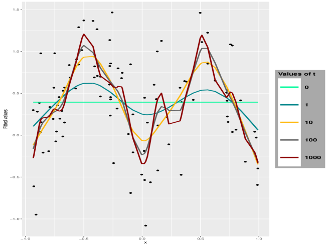
Figure 1: Output of the L²-Boosting algorithm in the vanishing learning rate asymptotic with input $(Y_{i},X_{i})_{1\leq i\leq 100}$ generated from model (26) at different values of $t$. The black dots represent the observed data set $(Y_{i},X_{i})_{1\leq i\leq 100}$.

To analyse this overfit and the effect of the learning rate $\lambda$, we then compare the training and test errors as defined in Section 2.3. In Figure 2 below, we plot the training and test errors of the boosting predictor $\hat{F}^{\lambda}_{[t/\lambda]}(\cdot)$ as a function of time $t\geq 0$ (in logarithmic scale), for different learning rates $\lambda=1$, $0.5$, $0.1$ and for the vanishing learning rate limit $\lambda\to 0$. We can see that the training error is decreasing while the test error decreases until a minimum at $t\approx\exp(1.8)\approx 6$ and starts to increase again. As $\lambda\to 0$, the error functions converge quickly to their limit and $\lambda=0.1$ can hardly be distinguished from the limit. Furthermore, convergence is slower for small time values and uniformly fast for large time values. Interestingly, the test error is minimal for vanishing learning rate $\lambda\to 0$, especially for small time values, supporting the idea that reducing the learning rate reduces the test error.

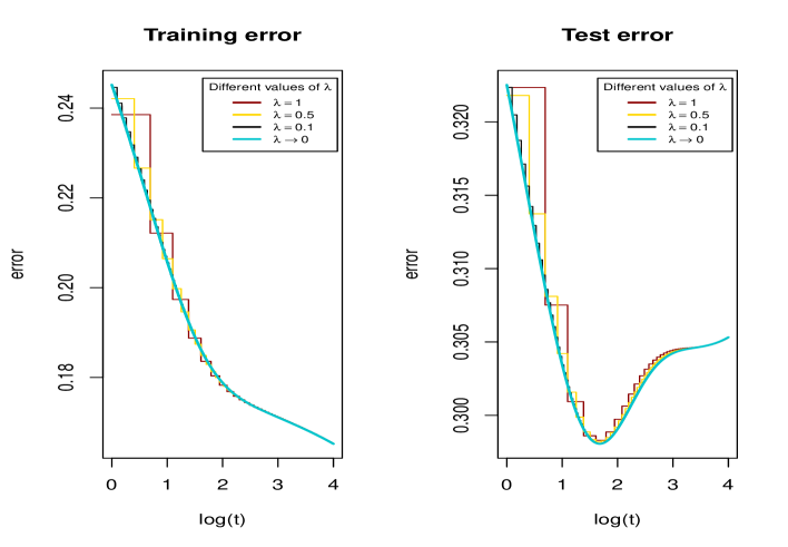
Figure 2: Training and test error of the predictors $\hat{F}_{t}(\cdot)$ and $\hat{F}^{\lambda}_{[t/\lambda]}(\cdot)$ for different values of $\lambda$.

Importantly, training error decreases slowly than expected, in contrast with the exponential rate of convergence announced by the theory. The convergence to $0$ of the training error cannot be observed on Figure 2 where $t$ ranges from $0$ to $\exp(4)\approx 50$. This phenomenon is explained by the order of magnitude of the eigenvalues of the base learner. The eigenvalues of $S$ quickly decrease to very small values as seen in Figure 3 below, where the $60$ largest eigenvalues are plotted in logarithmic scale (some numerical instability arises for smaller eigenvalues). The rate of convergence to $0$ of the training error is exponential with rate $e^{-t\mu_{100}}$, where $\mu_{100}$ denotes the smallest eigenvalues. Here we already have $\mu_{60}\approx 6\cdot 10^{-7}$ explaining the slow rate of decrease of the training error and the fact tjat convergence to zero is not observed in practice on usual time range.

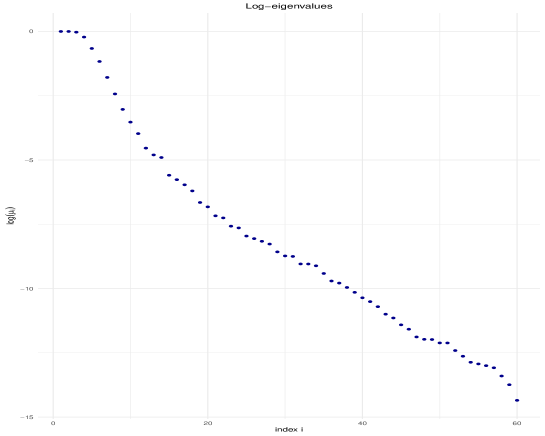
Figure 3: Decay of the base learner eigenvalues in logarithmic scale - only the $60$ largest eigenvalues are plotted due to numerical instability for smaller ones.

We next discuss what this behaviour of eigenvalues imply for the boosting predictor $\hat{F}_{t}(\cdot)$. When considering prediction at $\mathbf{x}=(x_{i})_{1\leq i\leq n}$, we can write $\hat{F}_{t}(\mathbf{x})=(\hat{F}_{t}(x_{i}))_{1\leq i\leq n}$ as

$$\hat{F}_{t}(\mathbf{x})=u_{1}u_{1}^{T}Y+\sum_{i=2}^{n}(1-e^{-\mu_{i}t})u_{i}u_{i}^{T}Y$$ (27)

where $(\mu_{i})_{1\leq i\leq n}$ and $(u_{i})_{1\leq i\leq n}$ are the eigenvalues and eigenvectors of $S$ and $Y=(Y_{i})_{1\leq i\leq n}$. The rank one matrix $u_{i}u_{i}^{T}$ is the matrix of the orthogonal projection on the eigenspace $\mathbb{R}u_{i}$. We interpret Equation (27) as a smoothed projection: for $\mu_{i}t\gg 1$, $1-e^{-\mu_{i}t}\approx 1$ and the boosting operator acts as the projection on this dimension; on the opposite, for $\mu_{i}t\ll 1$, $1-e^{-\mu_{i}t}\approx 0$ and the boosting operator acts as a filter on this dimension. The fact that the eigenvalues are spread out on multiple orders of magnitude implies that most of the coefficients are close to $0$ or $1$, whence the name smoothed projection. This is illustrated on Figure 4 where the coefficients from Equation (27) are plotted for various values of $t$. The sum of the coefficient is equal to the trace of the linear boosting operator, that is its number of degrees of freedom

$$\mathrm{df}(t)=1+\sum_{i=2}^{n}(1-e^{-\mu_{i}t}),$$

which is an increasing function of time. As we can see, boosting acts as a smoothed projection on the linear spaced spanned by the first eigenvectors. The larger the time, the larger the number of degrees of freedom of the smoothed projection, that is the larger the projection space.

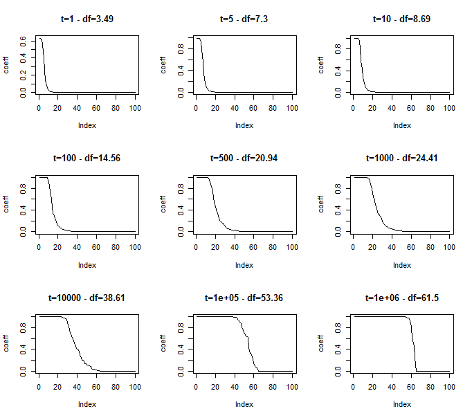
Figure 4: Coefficient appearing in Equation (27), the interpretation of the boosting linear operator as a smoothed projection.

We finally investigate the behaviour of the eigenvectors of base learner. Figures 5 and 6 respectively show the first and last eigenvectors. Quite strikingly, we can see that the first eigenvectors contains a well structured signal (akin to a polynomial basis) while the last eigenvectors mostly contains noise. The interpretation of linear boosting as a smoothed projection is thus meaningful as projection is performed on small dimensions containing signal, while higher dimensions associated to noise are filtered out.

Figure 5: First eigenvectors of the linear base learner interpreted as signal.

Figure 6: Last eigenvectors of the linear base learner interpreted as noise.

5 Proofs

5.1 Proofs for Section 2

Proof of Proposition 2.2.

A straightforward induction based on the recursive Equation (6) yields the first formula for $w_{m}^{\lambda}$. Furthermore, the identity

$$(I-\lambda S)\sum_{j=0}^{m-1}(I-\lambda S)^{j}=\sum_{j=0}^{m}(I-\lambda S)^{j}-I$$

implies

$$\lambda S\sum_{j=0}^{m-1}(I-\lambda S)^{j}=I-(I-\lambda S)^{m}.$$

When $S$ is invertible, we deduce

$$\lambda\sum_{j=0}^{m-1}(I-\lambda S)^{j}=S^{-1}[I-(I-\lambda S)^{m}]$$

and the second formula for $w_{m}^{\lambda}$ follows. ∎

Proof of Proposition 2.5.

Using the first formula for $w_{m}^{\lambda}$ from Proposition 2.2 and the binomial theorem, we get

$$w_{m}^{\lambda}=\lambda\sum_{j=0}^{m-1}\sum_{k=0}^{j}\binom{j}{k}\left(-\lambda S\right)^{k}\tilde{Y}=\lambda\sum_{k=0}^{m-1}\left(-\lambda S\right)^{k}\sum_{j=k}^{m-1}\binom{j}{k}\tilde{Y}.$$

By the Hockey-stick identity,

$$w_{m}^{\lambda}=\lambda\sum_{k=0}^{m-1}\binom{m}{k+1}\left(-\lambda S\right)^{k}\tilde{Y}=-\sum_{j=1}^{m}\binom{m}{j}(-\lambda)^{j}S^{j-1}\tilde{Y}.$$ (28)

Let $T>0$. In view of (5) and (9),

$$\sup_{t\in[0,T]}\sup_{x\in[0,1]^{p}}\left|\hat{F}_{\left[t/\lambda\right]}^{\lambda}(x)-\hat{F}_{t}(x)\right|\leq\sup_{t\in[0,T]}\sum_{i=1}^{n}\left|w_{\left[t/\lambda\right],i}^{\lambda}-w_{t,i}\right|\sup_{x\in[0,1]^{p}}\left|g_{i}(x)\right|.$$

The functions $g_{1},\ldots,g_{n}$ are locally bounded so that

$$\sup_{t\in[0,T]}\sup_{x\in[0,1]^{p}}\left|\hat{F}_{\left[t/\lambda\right]}^{\lambda}(x)-\hat{F}_{t}(x)\right|\leq M\sup_{t\in[0,T]}\left\|w_{\left[t/\lambda\right]}^{\lambda}-w_{t}\right\|$$ (29)

for some $M>0$. Here, $\|\cdot\|$ denotes any norm on $\mathbb{R}^{n}$ and we use below the same notation for the induced operator norm of $n\times n$ matrix. We need to prove that

$$\|w_{[t/\lambda]}^{\lambda}-w_{t}\|\to 0\quad\mbox{ uniformly for $t\in[0,T]$.}$$ (30)

Equation (28) implies

$$w_{\left[t/\lambda\right]}^{\lambda}-w_{t}=\sum_{j=1}^{\left[t/\lambda\right]}\left(\frac{(-t)^{j}}{j!}-\binom{\left[t/\lambda\right]}{j}(-\lambda)^{j}\right)S^{j-1}\tilde{Y}+\sum_{j>\left[t/\lambda\right]}\frac{(-t)^{j}}{j!}S^{j-1}\tilde{Y},$$

whence we deduce $\|w_{\left[t/\lambda\right]}^{\lambda}-w_{t}\|\leq\mathrm{I}+\mathrm{II}$ with

$$\mathrm{I} =\sum_{j=1}^{\left[t/\lambda\right]}\left|\frac{t^{j}}{j!}-\binom{\left[t/\lambda\right]}{j}\lambda^{j}\right|\left\|S\right\|^{j-1}\|\tilde{Y}\|,$$

$$\mathrm{II} =\sum_{j>\left[t/\lambda\right]}\frac{t^{j}}{j!}\|S\|^{j-1}\|\tilde{Y}\|.$$

Consider the first term. For $t\in[0,T]$, $\lambda>0$ and $1\leq j\leq[t/\lambda]$,

$$\binom{\left[t/\lambda\right]}{j}\lambda^{j}\geq\frac{1}{j!}\left(\lambda\left[t/\lambda\right]-\lambda(j-1)\right)^{j}\geq\frac{1}{j!}(t-\lambda j)^{j},$$

which entails

$$\left|\frac{t^{j}}{j!}-\binom{\left[t/\lambda\right]}{j}\lambda^{j}\right|\leq\frac{1}{j!}(t^{j}-(t-\lambda j)^{j})\leq\frac{1}{j!}(T^{j}-(T-\lambda j))^{j}$$

where the last inequality uses the fact that $t\mapsto t^{j}-(t-\lambda j)^{j}$ is increasing on $[\lambda j,+\infty)$. We deduce

$$\mathrm{I}\leq\|\tilde{Y}\|\sum_{j=1}^{\left[t/\lambda\right]}\frac{1}{j!}(T^{j}-(T-\lambda j)^{j})\|S\|^{j-1}.$$

Thanks to the inequality

$$T^{j}-(T-\lambda j)^{j}=\lambda j\sum_{k=0}^{j-1}T^{j-k-1}(T-\lambda j)^{k}\leq\lambda j^{2}T^{j-1},$$

we get the upper bound

$$\mathrm{I}\leq\lambda\|\tilde{Y}\|\sum_{j=1}^{\infty}\frac{1}{j!}j^{2}(T\|S\|)^{j-1}.$$

Since the last series converges and $t\in[0,T]$ is arbitrary, we deduce $\mathrm{I}=O(\lambda)$ as $\lambda\to 0$, uniformly for $t\in[0,T]$.

To analyze the second term, we distinguish between the case $t<\varepsilon$ and $t\geq\varepsilon$. For $t\in(0,\varepsilon]$,

$$\mathrm{II}\leq\|\tilde{Y}\|\sum_{j\geq 1}\frac{\varepsilon^{j}\|S\|^{j-1}}{j!}$$

and this can be made arbitrary small if we choose $\varepsilon$ small enough (independently of $\lambda$. On the other hand, for $t\in[\varepsilon,T]$,

$$\mathrm{II}\leq\|\tilde{Y}\|\sum_{j\geq\left[\delta/\lambda\right]}\frac{T^{j}\|S\|^{j-1}}{j!}$$

and the right hand side converges to $0$ as $\lambda\to 0$, because it is the remainder of a convergent series. We deduce that $\mathrm{II}\to 0$ as $\lambda\to 0$ uniformly in $t\in[0,T]$. This proves Equation (30) and, in view of Equation (29), the convergence $\hat{F}_{[t/\lambda]}^{\lambda}(x)\to\hat{F}_{t}(x)$ uniformly on $[0,T]\times[0,1]^{p}$.

Finally, in the case when $S$ is invertible, we have

$$w_{t} =-\sum_{j\geq 1}\frac{(-t)^{j}}{j!}S^{j-1}\tilde{Y}=-S^{-1}\sum_{j\geq 1}\frac{(-t)^{j}}{j!}S^{j}\tilde{Y}$$

$$=-S^{-1}(e^{-tS}-I)\tilde{Y}.$$

This proves Equation (11). ∎

Proof of Corollary 2.6.

When $S$ is symmetric, it can be written as the sum of rank $1$ orthogonal projections

$$S=\sum_{j=1}^{n}\mu_{j}u_{j}u_{j}^{\mathrm{T}}.$$

Then we have

$$\sum_{k\geq 1}\frac{(-t)^{k}}{k!}S^{k-1} =\sum_{j=1}^{n}\left(\sum_{k\geq 1}\frac{(-t)^{k}}{k!}\mu_{j}^{k-1}\right)u_{j}u_{j}^{\mathrm{T}}$$

$$=\sum_{j=1}^{n}\frac{e^{-\mu_{j}t}-1}{\mu_{j}}u_{j}u_{j}^{\mathrm{T}}$$

where the series are normally convergent and extension by continuity is used in the last equality when $\mu_{j}=0$. We deduce from Proposition 2.5 that

$$w_{t}=\sum_{j=1}^{n}\frac{1-e^{-\mu_{j}t}}{\mu_{j}}u_{j}u_{j}^{\mathrm{T}}\tilde{Y}$$

and Equation (12) follows from Equation (9) since $w_{t,i}=v_{i}^{\mathrm{T}}w_{t}$, $1\leq i\leq n$. ∎

Proof of Theorem 2.7.

We first check the claim that $\mathcal{L}$ is a bounded linear operator on $L^{\infty}$. We denote by $\|\cdot\|_{\infty}$ the norm in $L^{\infty}$. For all $x\in[0,1]^{p}$,

$$|\mathcal{L}(Z)(x)|\leq\sum_{i=1}^{n}|Z(x_{i})||g_{i}(x)|\leq\Big{\|}\sum_{i=1}^{n}|g_{i}|\Big{\|}_{\infty}\|Z\|_{\infty},$$

whence we deduce, taking the supremum over $x\in[0,1]^{p}$,

$$\|\mathcal{L}(Z)\|_{\infty}\leq\Big{\|}\sum_{i=1}^{n}|g_{i}|\Big{\|}_{\infty}\|Z\|_{\infty}.$$

This proves that the linear operator $\mathcal{L}$ is bounded.

Point $i)$ In the Banach space $L^{\infty}$, the differential equation (13) is linear of first order with constant bounded linear operator $\mathcal{L}$ and hence it follows from the general theory (see Apostol, (1969)) that it admits a unique solution starting from any point $Z_{0}$. We check that $Z(t)$ defined by Equation (14) is this solution. For $t=0$, $e^{-t\mathcal{L}}=\mathrm{Id}$ so that Equation (14) yields $Z(0)=Z_{0}$. On the other hand, differentiating Equation (14) thanks to the relations $(e^{-t\mathcal{L}})^{\prime}=-\mathcal{L}e^{-t\mathcal{L}}$, we obtain

$$Z^{\prime}(t) =-\mathcal{L}e^{-t\mathcal{L}}Z(0)+\mathcal{L}e^{-t\mathcal{L}}\mathcal{Y}$$

$$=-\mathcal{L}(Z(t)-(\mathrm{Id}-e^{-t\mathcal{L}})\mathcal{Y})+\mathcal{L}e^{-t\mathcal{L}}\mathcal{Y}$$

$$=-\mathcal{L}Z(t)+\mathcal{L}\mathcal{Y}$$

$$=-\mathcal{L}Z(t)+G.$$

In the last equality, we use the fact that $\mathcal{Y}$ is such that $\mathcal{L}(\mathcal{Y})=G$. This proves that $Z(t)$ is the solution of (13) with initial condition $Z(0)=Z_{0}$.

Point $ii)$ We finally check that $(\hat{F}_{t})_{t\geq 0}$ is the solution of (13) with initial condition $\bar{Y}_{n}$. By construction, we have $\hat{F}_{0}=\bar{Y}_{n}$. Furthermore, differentiating the relation

$$\hat{F}_{t}=\bar{Y}_{n}+\sum_{i=1}^{n}w_{t,i}g_{i}$$

yields

$$\hat{F}_{t}^{\prime}=\sum_{i=1}^{n}w_{t,i}^{\prime}g_{i}$$

where $w_{t,i}^{\prime}$ is the $i$-th component of

$$w_{t}^{\prime}=\sum_{j\geq 1}\frac{(-t)^{j-1}}{(j-1)!}S^{j-1}\tilde{Y}=e^{-tS}\tilde{Y}.$$

The derivative of $w_{t}$ is obtained by differenting the power series defining $w_{t}$ and we can see that $w_{t}$ satisfies the differential equation

$$w_{t}^{\prime}=-Sw_{t}+\tilde{Y},\quad t\geq 0.$$

As a consequence, for $t\geq 0$,

$$\hat{F}_{t}^{\prime} =\sum_{i=1}^{n}\Big{(}-\sum_{j=1}^{n}S_{i,j}w_{t,j}+\tilde{Y}_{i}\Big{)}g_{i}$$

$$=-\sum_{i=1}^{n}\Big{(}\bar{Y}_{n}+\sum_{j=1}^{n}w_{t,j}g_{j}(x_{i})\Big{)}g_{i}+\sum_{i=1}^{n}Y_{i}g_{i}$$

$$=-\sum_{i=1}^{n}\hat{F}_{t}(x_{i})g_{i}+\sum_{i=1}^{n}Y_{i}g_{i}$$

$$=-\mathcal{L}(\hat{F}_{t})+G.$$

This proves that $(\hat{F}_{t})_{t\geq 0}$ is the unique solution of Equation (13) starting from $\bar{Y}_{n}$ and its explicit form follows from point $ii)$. ∎

Proof of Proposition 2.11.

Using the linear independence of $g_{1},\ldots,g_{n}$ together with Equation (9), we can see that the output $\hat{F}_{t}$ remains bounded in $L^{\infty}$ as $t\to\infty$ if and only if the weight $w_{t}$ remains bounded in $\mathbb{R}^{n}$ as $t\to\infty$. Using the explicit formula (10) for $w_{t}$ and the Jordan decomposition of $S$, we prove that $(w_{t})_{t\geq 0}$ remains bounded if and only if, for all Jordan block $B$ of $S$,

$$\sum_{k\geq 1}\frac{(-t)^{k}}{k!}B^{k-1}\quad\mbox{remains bounded as $t\to\infty$}.$$ (31)

Indeed, the assumption $\sum_{i=1}^{n}g_{i}(x)=1$ implies that $1$ is an eigenvalue of $S$ associated to the constant eigenvector $1_{n}$. It follows that the centered input $\tilde{Y}$ in the definition of (10) can provide a contribution related to any other Jordan block.

Finally, we characterize the property (31). Write the Jordan block $B$ of size $s$ in the form $B=\mu I_{s}+N$ where $\mu$ is an eigenvalue of $S$ and $N$ a nilpotent matrix of order $s-1$. A standard discussion, akin to the criterion for the stability of linear systems of differential equations (see Bellman, (1969)), reveals that (31) holds if and only if $\mu$ has positive real part or if $s=1$ and $\mu$ has a null real part. ∎

Proof of Proposition 2.12.

Point $i)$. The convergence

$$\mathrm{err}_{train}(t)=\frac{1}{n}\|e^{-tS}\tilde{Y}\|\longrightarrow 0,\quad\mbox{as $t\to\infty$},$$

for all possible input is equivalent to the matrix convergence

$$e^{-tS}\longrightarrow 0,\quad\mbox{as $t\to\infty$}.$$

Note indeed that the centered input $\tilde{Y}$ belongs to the space orthogonal to $1_{n}$ but the direction $1_{n}$ is well-controlled since Assumption 2.10 implies $S1_{n}=1_{n}$ and hence $e^{-tS}1_{n}=e^{-t}1_{n}\to 0$. Finally, the convergence $e^{-tS}\longrightarrow 0$ is equivalent to the fact that all the (complex) eigenvalues of $S$ have a positive real part (see for example Bellman, (1997) and the references therein).

Point $ii)$. The relation

$$\mathbb{E}[\mathrm{err}_{train}(t)] =\frac{1}{n}\mathbb{E}[\|[R_{t}]\|^{2}]$$

$$=\frac{1}{n}\|\mathbb{E}[R_{t}]\|^{2}+\frac{1}{n}\mathrm{Trace}(\mathrm{Var}(R_{t})).$$ (32)

yields the decomposition into squared bias and variance. The vector of residuals is $R_{t}=e^{-tS}\tilde{Y}$ where $\tilde{Y}=(Y_{i}-\bar{Y}_{n})_{1\leq i\leq n}$ has expectation and variance

$$\mathbb{E}[\tilde{Y}] =f-\bar{f}1_{n}=\tilde{f},$$

$$\mathrm{Var}[\tilde{Y}] =\sigma^{2}\left(I-\frac{1}{n}1_{n}1_{n}^{T}\right)=\sigma^{2}J.$$

We deduce the squared bias and variance

$$\mathrm{bias}^{2}(t) =\frac{1}{n}\big{\|}\mathbb{E}[R_{t}]\big{\|}^{2}=\frac{1}{n}\big{\|}e^{-tS}\tilde{f}\big{\|}^{2},$$

$$\mathrm{var}_{train}(t) =\frac{1}{n}\mathrm{Trace}(\mathrm{Var}[R_{t}])=\frac{\sigma^{2}}{n}\mathrm{Trace}\big{(}e^{-tS}Je^{-tS^{T}}\big{)}$$

and Equation (18) follows from Equation (32).

Point $iii)$. When $S$ is symmetric, we use the decomposition $S=\sum_{i=1}^{n}\mu_{i}u_{i}u_{i}^{T}$ which implies

$$e^{-tS}\tilde{f}=\sum_{i=1}^{n}e^{-t\mu_{i}}(u_{i}^{T}\tilde{f})u_{i}$$

and

$$\mathrm{bias}^{2}(t)=\frac{1}{n}\|e^{-tS}\tilde{f}\|^{2}=\frac{1}{n}\sum_{i=1}^{n}e^{-2t\mu_{i}}(u_{i}^{T}\tilde{f})^{2}.$$

On the other hand, using furthermore the relations $S^{T}=S$, $\mathrm{Trace}(AB)=\mathrm{Trace}(BA)$ and $J^{2}=J$, we get

$$\mathrm{var}_{train}(t) =\frac{\sigma^{2}}{n}\mathrm{Trace}\Big{(}e^{-tS}Je^{-tS^{T}}\Big{)}=\frac{\sigma^{2}}{n}\mathrm{Trace}\Big{(}Je^{-2tS}J^{T}\Big{)}$$

$$=\frac{\sigma^{2}}{n}\sum_{i=1}^{n}e^{-2t\mu_{i}}\mathrm{Trace}\Big{(}Ju_{i}u_{i}^{T}J^{T}\Big{)}=\frac{\sigma^{2}}{n}\sum_{i=1}^{n}e^{-2t\mu_{i}}\|Ju_{i}\|^{2}.$$

∎

Proof of Proposition 2.13.

Point $i)$. The proof is similar to the proof of point $ii)$ in Proposition 2.12 and we give the main lines only. Equation (17) is equivalent to

$$\mathrm{err}_{test}(t)=\frac{1}{n}\big{\|}R_{t}^{\prime}\|^{2}\quad\mbox{with }R_{t}^{\prime}=(Y_{i}^{\prime}-\hat{F}_{t}(x_{i}))_{1\leq i\leq n},$$

so that $\mathbb{E}[\mathrm{err}_{test}(t)]=\mathrm{bias}^{2}(t)+\mathrm{var}_{test}(t)$ with

$$\mathrm{bias}^{2}(t) =\frac{1}{n}\big{\|}\mathbb{E}[R_{t}^{\prime}]\|^{2},$$

$$\mathrm{var}_{test}(t) =\frac{1}{n}\mathrm{Trace}(\mathrm{Var}(R_{t}^{\prime})).$$

Since $\mathbb{E}[R_{t}^{\prime}]=\mathbb{E}[R_{t}]=e^{-tS}\tilde{f}$, the squared bias is the same as in Proposition 2.12. Finally, the formula for the variance follows from the relation

$$R_{t}^{\prime}=Y^{\prime}+\bar{Y}_{n}1_{n}+(e^{-tS}-I)\tilde{Y}$$

where $Y^{\prime}=(Y^{\prime}_{i})_{1\leq i\leq n}$, $\bar{Y}_{n}1_{n}$ and $(e^{-tS}-I)\tilde{Y}$ are uncorrelated with variance $\sigma^{2}I$, $\sigma^{2}n^{-1}1_{n}1_{n}^{T}$ and $\sigma^{2}(I-e^{-tS})J(I-e^{-tS})^{T}$ respectively.

Point $ii)$. The formula are proved in the same way as the formulas of point $iii)$ in Proposition 2.12 and we omit the proof for the sake of brevity. The claimed properties of the squared bias and variance are straightforward. To prove the monotonicity of the expected test error near the origin and at infinity, it is enough to compute the derivative and prove that it is negative near $0$ and positive near infinity. The limit $2\sigma^{2}$ relies on the fact that $\sum_{i=1}^{n}\|Ju_{i}\|^{2}=n-1$ because $J$ is an orthogonal projection of rank $n-1$ and $(u_{i})_{1\leq i\leq n}$ and orthonormal basis. Details are left to the reader. ∎

Proof of Proposition 2.15.

Conditionally on $X^{\prime}=x^{\prime}$, we have the decomposition

$$\mathbb{E}[(Y^{\prime}-\hat{F}_{t}(X^{\prime}))^{2}\mid X^{\prime}=x^{\prime}] =\sigma^{2}+\mathbb{E}[(f(x^{\prime})-\hat{F}_{t}(x^{\prime}))^{2}]$$

$$=\sigma^{2}+(f(x^{\prime})-\mathbb{E}[F_{t}(x^{\prime})])^{2}+\mathrm{Var}[F_{t}(x^{\prime})].$$

By Proposition 2.5,

$$\hat{F}_{t}(x^{\prime})=\bar{Y}_{n}+g(x^{\prime})^{T}S^{-1}\left(I_{n}-\mathrm{e}^{-tS}\right)\tilde{Y},$$

with expectation and variance given by

$$\mathbb{E}[\hat{F}_{t}(x^{\prime})] =\bar{f}+g(x^{\prime})^{T}S^{-1}\left(I_{n}-\mathrm{e}^{-tS}\right)\tilde{f}$$

$$\mathrm{Var}[\hat{F}_{t}(x^{\prime})] =\frac{\sigma^{2}}{n}+g(x^{\prime})^{T}S^{-1}\left(I_{n}-\mathrm{e}^{-tS}\right)J_{n}\left(I_{n}-\mathrm{e}^{-tS}\right)S^{-1}g(x^{\prime}).$$

We deduce

$$\mathbb{E}[(Y^{\prime}-\hat{F}_{t}(X^{\prime}))^{2}\mid X^{\prime}=x^{\prime}]=\sigma^{2}+(f(x^{\prime})-\bar{f}-\tilde{f}^{T}S^{-1}\left(I_{n}-\mathrm{e}^{-tS}\right)g(x^{\prime}))^{2}$$

$$\quad\quad+\frac{\sigma^{2}}{n}+g(x^{\prime})^{T}S^{-1}\left(I_{n}-\mathrm{e}^{-tS}\right)J_{n}\left(I_{n}-\mathrm{e}^{-tS}\right)S^{-1}g(x^{\prime}).$$

Integrating with respect to $x^{\prime}$, we obtain the announced value of the test error. ∎

5.2 Proofs for Section 3

Proof of Proposition 3.4.

As a preliminary, we state a Markov property of the stochastic boosting algorithm. For $x\in[0,1]^{p}$, we note $\mathbf{x}=(x_{i})_{1\leq i\leq n+1}$ with the convention $x_{n+1}=x$ and also $\hat{F}_{m}^{\lambda}(\mathbf{x})=(\hat{F}_{m}^{\lambda}(x_{i}))_{1\leq i\leq n+1}$. We observe that $(\hat{F}_{m}^{\lambda}(\mathbf{x}))_{m\geq 0}$ is a time homogeneous Markov chain with values in $\mathbb{R}^{n+1}$. Indeed, the recursive relation (19) implies that $\hat{F}_{m+1}^{\lambda}(\mathbf{x})$ depends only of $(\hat{F}_{m}^{\lambda}(x_{i}))_{1\leq i\leq n}$, and $\xi_{m+1}$. The time homogeneous Markov property follows since $\hat{F}_{m}^{\lambda}(\bf x)$ contains $(\hat{F}_{m}^{\lambda}(x_{i}))_{1\leq i\leq n}$ in its first $n$ components and $\xi_{m+1}$ is independent on the past $\hat{F}_{0}^{\lambda}(\mathbf{x}),\ldots,\hat{F}_{m}^{\lambda}(\mathbf{x})$.

Point $i)$. Taking conditional expectation, Equation (19) implies

$$\mathbb{E}_{\xi}[\hat{F}_{m+1}^{\lambda}(\mathbf{x})\mid\hat{F}_{m}^{\lambda}(\mathbf{x})]=\hat{F}_{m}^{\lambda}(\mathbf{x})+\lambda\sum_{i=1}^{n}(Y_{i}-\hat{F}_{m}^{\lambda}(x_{i}))\bar{g}_{i}(\mathbf{x}),\quad m\geq 0,$$ (33)

with $\bar{g}_{j}(\mathbf{x})=(\bar{g}_{j}(x_{i}))_{1\leq i\leq n+1}$. We deduce

$$\mathbb{E}_{\xi}[\hat{F}_{m+1}^{\lambda}(\mathbf{x})]=\mathbb{E}_{\xi}[\hat{F}_{m}^{\lambda}(\mathbf{x})]+\lambda\sum_{i=1}^{n}(Y_{i}-\mathbb{E}_{\xi}[\hat{F}_{m}^{\lambda}(x_{i})])\bar{g}_{i}(\mathbf{x}),\quad m\geq 0.$$

Considering component $n+1$, we see that the functions $x\mapsto\mathbb{E}_{\xi}[\hat{F}_{m+1}^{\lambda}(x)]$ satisfy the recursive relation (2) where the linear base learner is given by (4) with $g_{j}$ replaced by $\bar{g}_{j}$. Proposition 2.2 then yields the explicit form for $\mathbb{E}_{\xi}[\hat{F}_{m+1}^{\lambda}(\mathbf{x})]$ stated in Equation (21).

Point $ii)$. In order to compute the variance of $\hat{F}_{m}^{\lambda}(x_{j})$, $1\leq j\leq n+1$, we use the recursive relation (2) together with the variance decomposition

$$\mathrm{Var}_{\xi}[\hat{F}_{m+1}^{\lambda}(x_{j})]=\mathrm{Var}_{\xi}[\mathbb{E}_{\xi}[\hat{F}_{m+1}^{\lambda}(x_{j})\mid\hat{F}_{m}^{\lambda}(\mathbf{x})]]+\mathbb{E}_{\xi}[\mathrm{Var}_{\xi}[\hat{F}_{m+1}^{\lambda}(x_{j})\mid\hat{F}_{m}^{\lambda}(\mathbf{x})]].$$

In view of Equation (33), the first term satisfies

$$\mathrm{Var}_{\xi}[\mathbb{E}_{\xi}[\hat{F}_{m+1}^{\lambda}(x_{j})\mid\hat{F}_{m}^{\lambda}(\mathbf{x})]]$$

$$=\mathrm{Var}_{\xi}\Big{[}\hat{F}_{m}^{\lambda}(x_{j})+\lambda\sum_{i=1}^{n}(Y_{i}-\hat{F}_{m}^{\lambda}(x_{i}))\bar{g}_{i}(x_{j})\Big{]}$$

$$=\mathrm{Var}_{\xi}[\hat{F}_{m}^{\lambda}(x_{j})]+\lambda^{2}\sum_{1\leq i,k\leq n}\bar{g}_{i}(x_{j})\bar{g}_{k}(x_{j})\mathrm{Cov}_{\xi}[\hat{F}_{m}^{\lambda}(x_{i}),\hat{F}_{m}^{\lambda}(x_{k})]$$

$$\quad-2\lambda\sum_{i=1}^{n}\bar{g}_{i}(x_{j})\mathrm{Cov}_{\xi}[\hat{F}_{m}^{\lambda}(x_{j}),\hat{F}_{m}^{\lambda}(x_{i})]$$

$$\leq\left(1+\lambda M_{1}\right)^{2}\max_{1\leq i\leq n+1}\mathrm{Var}_{\xi}[\hat{F}_{m}^{\lambda}(x_{i})],$$

where $M_{1}$ is given by Equation (22). In the last inequality, we use the Cauchy-Schwartz inequality to upper bound the covariances. We next provide an upper bound for the second term in the variance decomposition. We have

$$\mathrm{Var}_{\xi}[\hat{F}_{m+1}^{\lambda}(x_{j})\mid\hat{F}_{m}^{\lambda}(\mathbf{x})]$$

$$=\lambda^{2}\mathrm{Var}_{\xi}\Big{[}\sum_{i=1}^{n}(Y_{i}-\hat{F}_{m}^{\lambda}(x_{i}))g_{i}(x_{j})\mid\hat{F}_{m}^{\lambda}(\mathbf{x})\Big{]}$$

$$=\lambda^{2}\sum_{1\leq i,k\leq n}(Y_{i}-\hat{F}_{m}^{\lambda}(x_{i}))(Y_{k}-\hat{F}_{m}^{\lambda}(x_{k}))\mathrm{Cov}_{\xi}[g_{i}(x_{j}),g_{k}(x_{j})]$$

$$\leq\lambda^{2}M_{2}\sum_{i=1}^{n}(Y_{i}-\hat{F}_{m}^{\lambda}(x_{i}))^{2},$$

where $M_{2}$ is defined in (23). The last line relies on the inequality $u^{T}\Sigma u\leq\rho(\Sigma)\|u\|^{2}$, where $u\in\mathbb{R}^{n}$, $\Sigma\in\mathbb{R}^{n\times n}$ is a non negative symmetric matrix and $\rho(\Sigma)$ denotes its spectral radius, i.e. its largest eigenvalue. We apply this inequality with $u=(Y_{i}-\hat{F}_{m}^{\lambda}(x_{i}))_{1\leq i\leq n}$ and $\Sigma=(\mathrm{Cov}_{\xi}[g_{i}(x_{j}),g_{k}(x_{j})])$ and we use the fact that $\rho(\Sigma)\leq\mathrm{Trace}(\Sigma)$. We deduce that the second term in the variance decomposition is upper bounded by

$$\mathbb{E}_{\xi}[\mathrm{Var}_{\xi}[\hat{F}_{m+1}^{\lambda}(x_{j})\mid\hat{F}_{m}^{\lambda}(\mathbf{x})]]$$

$$\leq\lambda^{2}M_{2}\sum_{i=1}^{n}\mathbb{E}_{\xi}[(Y_{i}-\hat{F}_{m}^{\lambda}(x_{i}))^{2}]$$

$$\leq n\lambda^{2}M_{2}\max_{1\leq i\leq n+1}\mathrm{Var}_{\xi}[\hat{F}_{m}^{\lambda}(x_{i})]+\lambda^{2}M_{2}\sum_{i=1}^{n}(Y_{i}-\mathbb{E}_{\xi}[\hat{F}_{m}^{\lambda}(x_{i})])^{2}.$$

Collecting the two terms of the variance decomposition, we get

$$\mathrm{Var}_{\xi}[\hat{F}_{m+1}^{\lambda}(x_{j})]\leq(1+\alpha)a_{m}+\beta b_{m}$$

with $\alpha=2\lambda M_{1}+\lambda^{2}M_{1}^{2}+n\lambda^{2}M_{2}$, $\beta=\lambda^{2}M_{2}$, $a_{m}=\max_{1\leq i\leq n+1}\mathrm{Var}_{\xi}[\hat{F}_{m}^{\lambda}(x_{i})]$ and $b_{m}=\sum_{i=1}^{n}(Y_{i}-\mathbb{E}_{\xi}[\hat{F}_{m}^{\lambda}(x_{i})])^{2}$. Taking the maximum over $j=1,\ldots,n+1$, note that the sequence $(a_{m})_{m\geq 0}$ satisfies

$$a_{m+1}\leq(1+\alpha)a_{m}+\beta b_{m},\quad m\geq 0.$$

By the discrete Gronwall lemma or a straightforward induction, we deduce

$$a_{m}\leq(1+\alpha)^{m+1}a_{0}+\beta(1+\alpha)^{m}\sum_{k=0}^{m}b_{k},\quad m\geq 0.$$

We use now Equations (21) and (28) to show that

$$b_{k} \leq 2\sum_{i=1}^{n}(Y_{i}-\bar{Y}_{n})^{2}+2nM_{1}^{2}\left(\max_{1\leq i\leq n}\left|w_{k,i}^{\lambda}\right|\right)^{2}$$

$$\leq 2n\|\tilde{Y}\|_{\infty}^{2}+2nM_{1}^{2}\left(\sum_{j=1}^{k}\binom{k}{j}\lambda^{j}\|S\|_{\infty}^{j-1}\|\tilde{Y}\|_{\infty}\right)^{2}$$

$$\leq 2n\|\tilde{Y}\|_{\infty}^{2}+2nM_{1}^{2}\|\tilde{Y}\|_{\infty}^{2}\left(\lambda k\sum_{j=1}^{k}\frac{(\lambda k\|S\|_{\infty})^{j-1}}{(j-1)!}\right)^{2}$$

$$\leq 2n\|\tilde{Y}\|_{\infty}^{2}\left\{1+(\lambda kM_{1})^{2}\mathrm{e}^{2\lambda k\|S\|_{\infty}}\right\}.$$

This implies that

$$\sum_{k=0}^{m}b_{k}\leq 2(m+1)n\|\tilde{Y}\|_{\infty}^{2}\left\{1+(\lambda mM_{1})^{2}\mathrm{e}^{2\lambda m\|S\|_{\infty}}\right\}.$$

Therefore, as $a_{0}=0$, it follows that

$$\max_{1\leq i\leq n+1}\mathrm{Var}_{\xi}[\hat{F}_{m}^{\lambda}(x_{i})] \leq 2(m+1)\beta(1+\alpha)^{m}n\|\tilde{Y}\|_{\infty}^{2}\left\{1+(\lambda mM_{1})^{2}\mathrm{e}^{2\lambda m\|S\|_{\infty}}\right\}.$$

Since, for $\lambda<1$, $\alpha\leq(2M_{1}+M_{1}^{2}+(n+1)M_{2})\lambda$ and $2\beta\leq(2M_{1}+M_{1}^{2}+(n+1)M_{2})\lambda^{2}$, the expected upper bound for the variance of the stochastic boosting output $\hat{F}_{m}^{\lambda}(x)$ is obtained. ∎

Proof of Corollary 3.5.

First observe that

$$\lim_{\lambda\to 0}\mathbb{E}_{\xi}[\hat{F}_{[t/\lambda]}^{\lambda}(x)]=\bar{Y}_{n}+\sum_{i=1}^{n}w_{t,i}\bar{g}_{i}(x)=\hat{F}_{t}(x).$$

This is a straightforward consequence of Equation (21) and of the weight convergence $w_{[t/\lambda]}^{\lambda}\to w_{t}$ stated in Proposition 2.5. Together with the convergence of the variance $\mathrm{Var}_{\xi}[\hat{F}_{[t/\lambda]}^{\lambda}(x)]\to 0$ deduced from point $ii)$ of Proposition 3.4, this yields the convergence in quadratic mean $\hat{F}_{[t/\lambda]}^{\lambda}(x)\to\hat{F}_{t}(x)$ as $\lambda\to 0$. ∎

Proof of Theorem 3.6.

Point $i)$. The recursive relation (19) can be rewritten as

$$\hat{F}_{m+1}^{\lambda}=T(\hat{F}_{m}^{\lambda},\xi_{m+1}),\quad m\geq 0,$$

with $T:L^{\infty}\times\Xi\to L^{\infty}$ defined by

$$T(F,\xi)=F(\cdot)+\lambda\sum_{i=1}^{n}(Y_{i}-F(x_{i}))g_{i}(\cdot,\xi).$$

Since $(\xi_{m})_{m\geq 1}$ is i.i.d. and independent of $(x_{i})_{1\leq i\leq n}$, $(Y_{i})_{1\leq i\leq n}$ and $\hat{F}_{0}^{\lambda}=\bar{Y}_{n}$, this implies that $(\hat{F}_{m}^{\lambda})_{m\geq 0}$ is a time homogeneous Markov chain.

Point $ii)$. Note that the Markov chain $(\hat{F}_{m}^{\lambda})_{m\geq 0}$ remains in the finite dimensional subspace

$$\mathcal{F}=\mathrm{span}(1,g_{i}(\cdot,\xi);1\leq i\leq n,\xi\in\Xi)\subset L^{\infty}$$

and that the Markov property stated in point $i)$ remains true if we replace $L^{\infty}$ by the subspace $\mathcal{F}$. We apply Theorem 11.2.3 in Stroock and Varadhan, (2006), page 272, to the Markov chain $(\hat{F}_{m}^{\lambda})_{m\geq 0}$ on $\mathcal{F}$. Let $f\in\mathcal{F}$ and consider the local drift and volatility of the Markov chain at $f$ defined respectively by

$$b_{\lambda}(f) =\lambda^{-1}\mathbb{E}_{\xi}[\hat{F}_{m}+1^{\lambda}-\hat{F}_{m}^{\lambda}\mid\hat{F}_{m}^{\lambda}=f]$$

$$a_{\lambda}(f) =\lambda^{-1}\mathbb{E}_{\xi}[(\hat{F}_{m+1}^{\lambda}-\hat{F}_{m}^{\lambda})(\hat{F}_{m+1}^{\lambda}-\hat{F}_{m}^{\lambda})^{T}\mid\hat{F}_{m}^{\lambda}=f]$$

where $f$ is implicitly identified with its vector of coordinates in some basis so that the product $ff^{T}$ makes sense.

Given $\hat{F}_{m}^{\lambda}=f$, we have

$$\hat{F}_{m+1}^{\lambda}-\hat{F}_{m}^{\lambda}=\lambda\sum_{i=1}^{n}(Y_{i}-f(x_{i}))g_{i}(\cdot,\xi_{m+1}).$$

We deduce that the local drif is given by

$$b_{\lambda}(f)=\sum_{i=1}^{n}(Y_{i}-f(x_{i}))\bar{g}_{i}$$

and does not depend on $\lambda$, i.e. $b_{\lambda}(f)=b(f)$.

To deal with the local volatility $a_{\lambda}(f)$, note first that there exists a constant $C>0$ such that the matrix $ff^{T}$ has all its coefficients bounded by $C\|f\|_{\infty}^{2}$. This is a consequence of the equivalence of norms on the finite dimensional space $\mathcal{F}$: the norm $\|\cdot\|_{\infty}$ is equivalent to the norm of the vector representing $f$ in the basis implicitly used for computing $ff^{T}$. We can thus bound the coefficients of the local volatility matrix by

$$\lambda C\mathbb{E}_{\xi}\Big{\|}\sum_{i=1}^{n}(Y_{i}-f(x_{i}))g_{i}(\cdot,\xi_{m+1})\Big{\|}_{\infty}^{2}$$

$$\leq\lambda CM^{2}\Big{(}\max_{1\leq i\leq n}\left|Y_{i}-f(x_{i})\right|\Big{)}^{2},$$

where $M=\max_{\xi\in\Xi}\|\sum_{i=1}^{n}|g_{i}(\cdot,\xi)|\|_{\infty}$ is finite because $\Xi$ is finite. We deduce

$$a^{\lambda}(f)\longrightarrow a(f)\equiv 0\quad\mbox{uniformly on compact sets as $\lambda\to 0$.}$$

The limit functions $a$ and $b$ are continuous. Since $a\equiv 0$ and $b$ is an affine function, the associated martingale problem has exactly one solution starting from any point, see Stroock and Varadhan, (2006) Lemma 6.1.4 page 140 or Theorem 6.3.4 page 152. In fact, because the limit volatility $a\equiv 0$ is vanishing, the solution of the martingale problem is the solution of the differential equation on $\mathcal{F}$

$$f^{\prime}(t)=b(f(t))=\sum_{i=1}^{n}(Y_{i}-f(x_{i}))\bar{g}_{i},\quad t\geq 0.$$

This is exactly the differential Equation (13) and we have proved in Theorem 2.7 that it has a unique solution with initial condition $f(0)=\bar{Y}_{n}$. Then, Theorem 11.2.3 in Stroock and Varadhan, (2006) implies that the continous processes defined by interpolation

$$\tilde{F}_{t}^{\lambda}=(1-\{t/\lambda\})\hat{F}_{[t/\lambda]}^{\lambda}+\{t/\lambda\}\hat{F}_{[t/\lambda]+1}^{\lambda},\quad t\geq 0,$$

converge in distribution in the space of continuous functions $\mathbb{C}([0,\infty),\mathcal{F})$

$$(\tilde{F}_{t}^{\lambda})_{t\geq 0}\stackrel{{\scriptstyle d}}{{\longrightarrow}}(\hat{F}_{t})_{t\geq 0}.$$ (34)

The notation $\{u\}=u-[u]$ stands for the fractional part of a real number. Finally, the convergence in distribution (25) in the Skorokhod space $\mathbb{D}([0,\infty),\mathcal{F})$ follows by a standard discretization argument. It holds

$$(\hat{F}^{\lambda}_{[t/\lambda]})_{t\geq 0}=\Psi_{\lambda}((\tilde{F}^{\lambda}_{t})_{t\geq 0})$$

where $\Psi_{\lambda}:\mathbb{C}([0,\infty),\mathcal{F})\longrightarrow\mathbb{D}([0,\infty),\mathcal{F})$ is the discretization functional

$$\Psi_{\lambda}((f_{t})_{t\geq 0})=(f_{\lambda[t/\lambda]})_{t\geq 0}.$$

The functional $\Psi_{\lambda}$ satisfies the following property: for all converging sequence $(f_{t}^{\lambda})\to(f_{t})$ in $\mathbb{C}([0,\infty),\mathcal{F})$ as $\lambda\to 0$, it holds $\Psi_{\lambda}((f_{t}^{\lambda}))\to(f_{t})$ in $\mathbb{D}([0,\infty),\mathcal{F})$ as $\lambda\to 0$. Together with the convergence (34), this implies the convergence (25) by the generalized continuous mapping theorem (Billingsley,, 1999, Theorem 2.7). ∎

References

- Apostol, (1969) Apostol, T. (1969). Calculus. Vol. II: Multi-variable Calculus and Linear Algebra, with Applications to Differential Equations and Probability. Blaisdell international textbook series. Xerox College Publ.
- Bartlett and Traskin, (2007) Bartlett, P. L. and Traskin, M. (2007). AdaBoost is consistent. J. Mach. Learn. Res., 8:2347–2368.
- Bellman, (1969) Bellman, R. (1969). Stability Theory of Differential Equations. Dover books on intermediate and advanced mathematics. Dover Publications.
- Bellman, (1997) Bellman, R. (1997). Introduction to Matrix Analysis: Second Edition. Classics in Applied Mathematics. Society for Industrial and Applied Mathematics.
- Bergstra et al., (2006) Bergstra, J., Casagrande, N., Erhan, D., Eck, D., and Kégl, B. (2006). Aggregate features and adaboost for music classification. Machine Learning, 65:473–484.
- Billingsley, (1999) Billingsley, P. (1999). Convergence of probability measures. Wiley Series in Probability and Statistics: Probability and Statistics. John Wiley & Sons, Inc., New York, second edition. A Wiley-Interscience Publication.
- Breiman, (2004) Breiman, L. (2004). Population theory for boosting ensembles. Ann. Statist., 32(1):1–11.
- Bühlmann and Yu, (2003) Bühlmann, P. and Yu, B. (2003). Boosting with the loss: regression and classification. J. Amer. Statist. Assoc., 98(462):324–339.
- Dudoit et al., (2002) Dudoit, S., Yang, Y. H., Callow, M. J., and Speed, T. P. (2002). Statistical methods for identifying differentially expressed genes in replicated cdna microarray experiments. Statistica Sinica, 12(1):111–139.
- Ethier and Kurtz, (1986) Ethier, S. N. and Kurtz, T. G. (1986). Markov processes. Wiley Series in Probability and Mathematical Statistics: Probability and Mathematical Statistics. John Wiley & Sons, Inc., New York. Characterization and convergence.
- Freund and Schapire, (1999) Freund, Y. and Schapire, R. (1999). Adaptive game playing using multiplicative weights. volume 29, pages 79–103. Learning in games: a symposium in honor of David Blackwell.
- Friedman et al., (2000) Friedman, J., Hastie, T., and Tibshirani, R. (2000). Additive logistic regression: a statistical view of boosting. Ann. Statist., 28(2):337–407. With discussion and a rejoinder by the authors.
- Friedman, (2001) Friedman, J. H. (2001). Greedy function approximation: a gradient boosting machine. Annals of statistics, pages 1189–1232.
- Friedman, (2002) Friedman, J. H. (2002). Stochastic gradient boosting. Computational statistics & data analysis, 38(4):367–378.
- Horn and Johnson, (2013) Horn, R. and Johnson, C. (2013). Matrix analysis. Cambridge University Press, Cambridge, second edition.
- Nadaraya, (1964) Nadaraya, E. A. (1964). On estimating regression. Theory of Probability & Its Applications, 9(1):141–142.
- Ridgeway, (2007) Ridgeway, G. (2007). Generalized boosting models: a guide to the gbm package. URL https://cran.r-project.org/web/packages/gbm/vignettes/gbm.pdf.
- Stroock and Varadhan, (2006) Stroock, D. W. and Varadhan, S. R. S. (2006). Multidimensional diffusion processes. Classics in Mathematics. Springer-Verlag, Berlin. Reprint of the 1997 edition.
- Wahba, (1990) Wahba, G. (1990). Spline Models for Observational Data. CBMS-NSF Regional Conference Series in Applied Mathematics. Society for Industrial and Applied Mathematics.
- Watson, (1964) Watson, G. S. (1964). Smooth regression analysis. Sankhya: The Indian Journal of Statistics, Series A (1961-2002), 26(4):359–372.
- Zhang and Yu, (2005) Zhang, T. and Yu, B. (2005). Boosting with early stopping: convergence and consistency. Ann. Statist., 33(4):1538–1579.