New fit of time-like proton electromagnetic form factors from $e^{+}e^{-}$ colliders

Abstract

The data on the proton form factors in the time-like region from the BaBar, BESIII and CMD-3 Collaborations are examined to have coherent pieces of information on the proton structure. Oscillations in the annihilation cross section, previously observed, are determined with better precision. The moduli of the individual form factors, determined for the first time, their ratio and the angular asymmetry of the annihilation reaction $e^{+}e^{-}\to\bar{p}p$ are discussed. Fiits of the available data on the cross section, the effective form factor, and the form factor ratio, allow to propose a description of the electric and magnetic time-like form factors from the threshold up to the highest momenta.

I Introduction

The understanding of the proton electromagnetic form factors (FFs), called electric $G_{E}(q^{2})$ and magnetic $G_{M}(q^{2})$ Sachs FFs is the aim of theoretical and experimental studies since decades, in the frame of a unified view of the scattering and annihilation regions. Much progress has been done recently, due, on one side, to new experiments that collected information with better precision and/or in a wider kinematical range and, on the other side, to theoretical efforts that extend models and parametrizations built in the space-like (SL) region to the time-like (TL) region (for a review, see Ref. Pacetti et al. (2015)). We discuss here the data on the $e^{+}e^{-}\to\bar{p}p$ cross section, $\sigma_{e^{+}e^{-}\to\bar{p}p}$, from the BaBar, BESIII and CMD-3 Collaborations, obtained either by direct measurements of the annihilation process, or by means of the so-called initial state radiation (ISR) technique, $i.e.$, by exploiting the three-body process $e^{+}e^{-}\to\bar{p}p\gamma$, where the photon is radiated by one of the initial leptons.

The emission of a real hard photon, leaving the radiating lepton in a “quasi-real” state, allows extracting the cross section for the process $e^{+}e^{-}\to\bar{p}p$ from the differential cross section of the three-body process $e^{+}e^{-}\to\bar{p}p\gamma$. In such a kinematic domain, $\sigma_{e^{+}e^{-}\to\bar{p}p}$ factorizes out in the expression of the ISR differential cross section. In collinear kinematics, the ISR cross section manifests a logarithmic enhancement as a consequence of the small mass of the virtual electron that is almost on mass shell Baier et al. (1973). At fixed energy colliders the ISR technique allows to extract values of the $\sigma_{e^{+}e^{-}\to\bar{p}p}$ cross section at different transferred momenta, $i.e.,$ different values of $q^{2}$ (being $q$ the four-momentum of the virtual photon in the annihilation reaction $e^{+}e^{-}\to\bar{p}p$) by tuning the kinematics of the real photon. The cost is a reduction of a factor of $\alpha=e^{2}/(4\pi)\simeq 1/137$ (the electromagnetic fine constant) of the number of events, that, however, can be compensated by the high luminosity recently achieved at the experimental facilities.

By means of the ISR technique and detecting the radiated hard photon, the BaBar Collaboration obtained data on the $e^{+}e^{-}\to\bar{p}p$ cross section with an error lower than 10% in a wide energy region, from the production threshold $\sqrt{s}=2m_{p}$ up to $\sqrt{s}\leavevmode\nobreak\ \simeq\leavevmode\nobreak\ 6$ GeV Lees et al. (2013a), where $s=q^{2}$ is the total energy squared in the center of mass (CM) frame of the $\bar{p}p$-system and $m_{p}$ is the proton mass. Recently, using the same technique but with undetected initial photon, the BESIII Collaboration extracted 30 values of $\sigma_{e^{+}e^{-}\to\bar{p}p}$ in the range $(2\leq\sqrt{s}\leq 3.8)$ GeV Ablikim et al. (2019). The ISR photon is undetected, $i.e.$, it is mostly emitted at small polar angles in a kinematical region uncovered by BESIII acceptance. This method was also used by the BaBar Collaboration, where the hard condition of the photon was insured by high energy of the colliding beams Lees et al. (2013b).

The individual determination of the moduli of the FFs in the TL region was done by the BESIII Collaboration, using the energy scan method Ablikim et al. (2020), with a precision comparable to that of the data obtained in the SL scattering region. The data in the SL region were mostly collected by the JLab GEp Collaboration and published in a series of papers, summarized in Refs. Puckett et al. (2017, 2012). The BESIII Collaboration has made the individual measurement of $|G_{E}|$ and $|G_{M}|$, separately, in the TL region for the first time ever.

In fact, before such a pioneering measurement, the few information on the FF moduli in the TL region concerned a composed observable, namely their ratio $R=|G_{E}|/|G_{M}|$, extracted from angular distribution measurements. Due to luminosity limitations, only an ’effective form factor’ could be extracted from the total cross section.

Let us stress that only the moduli of the FFs, which, in principle, have a non-vanishing imaginary part in the TL region, can be extracted from a precise large-statistics measurement of the angular distribution of the final-state nucleons in the $e^{+}e^{-}$-CM frame. The underlying assumption is that the reaction occurs through the one-photon exchange mechanism Zichichi et al. (1962). No measurement of the relative phase between $G_{E}$ and $G_{M}$, accessible through polarization observables Dubnickova et al. (1996), is available yet for protons and neutrons .

Focussed on the threshold region, the CMD-3 Collaboration Akhmetshin et al. (2019) measured the cross section for the reactions $e^{+}e^{-}\to\bar{p}p\gamma$ and $e^{+}e^{-}\to\bar{n}n\gamma$. The scan of the nucleon-antinucleon threshold energy region is done by measuring the beam energy at 0.1 MeV precision by back-scattering laser light system. The energy spread due to radiation and energy resolution is small enough to differentiate the proton and neutron thresholds.

The aim of the present work is to scrutinize the recent data on proton FFs in TL region, through the reaction $e^{+}e^{-}\to\bar{p}p(\gamma)$. Two characteristics, earlier predicted or highlighted, can be confirmed or infirmed by the new data: the finding of regular oscillations of the cross section Bianconi and Tomasi-Gustafsson (2015) and the steeper $q^{2}$-dependence of the electric FF ($G_{E}$) compared to the magnetic FF ($G_{M}$), as found in the SL region Jones et al. (2000); Puckett et al. (2017). The suggestion of a similar $q^{2}$-dependence in space and TL regions is based on analytical properties of the amplitudes Tomasi-Gustafsson and Rekalo (2001) and illustrated in frame of a generalized definition of FFs Kuraev et al. (2012).

Not all models developed in the SL region have the correct analytical properties to be extended in the TL region, where FFs are of complex nature Tomasi-Gustafsson et al. (2005). Models based on dispersion relations Belushkin et al. (2007) or vector dominance Bijker and Iachello (2004); Lomon and Pacetti (2012) have attempted a global description in SL and TL regions, for a review, see Refs. Pacetti et al. (2015); Denig and Salme (2013). In this paper we consider the new data and we propose a global fit from threshold up to the maximum available transferred momentum. The individual TL FFs are reproduced from a fit on the ratio $R$ and of the effective FF, allowing to extrapolate their behavior at threshold, where $R$ is constrained to unity.

II The $e^{+}e^{-}\to\bar{p}p(\gamma)$ cross section

As already pointed out, at fixed-energy $e^{+}e^{-}$-colliders, the $e^{+}e^{-}\to\bar{p}p$ cross section, can be extracted from the data on the differential cross section of the ISR process $e^{+}e^{-}\to\bar{p}p\gamma$, where the photon is radiated by one of the initial electrons, over a range of $\bar{p}p$-energies going from the threshold, $\sqrt{s_{\mathrm{thr}}}=2m_{p}$, up to the full $e^{+}e^{-}$ CM energy, $\sqrt{s_{e^{+}e^{-}}}$. Similar formalism can be applied for the annihilation $e^{+}e^{-}\to\bar{n}n$.

In Ref. Lees et al. (2013a), based on the work of Ref. Bonneau and Martin (1971), the differential cross section for the radiative process, integrated over the nucleon momenta, was factorized into a function which depends on the photon kinematical variables multiplied by the annihilation cross section of interest, for the process $e^{+}e^{-}\rightarrow\bar{p}p$:

$$\frac{d^{2}\sigma_{e^{+}e^{-}\to\bar{p}p\gamma}}{d\sqrt{s_{e^{+}e^{-}}}\,d\cos(\theta_{\gamma})}=\displaystyle\frac{2\sqrt{s}}{s_{e^{+}e^{-}}}W(s_{e^{+}e^{-}},E_{\gamma},\theta_{\gamma})\sigma_{e^{+}e^{-}\to\bar{p}p}(s)\,,\hskip 28.45274ptE_{\gamma}=\frac{s-s_{e^{+}e^{-}}}{2\sqrt{s_{e^{+}e^{-}}}}\,,$$ (1)

where $\sqrt{s}$ and $\sqrt{s_{e^{+}e^{-}}}$ are the invariant masses of the $\bar{p}p$ and $e^{+}e^{-}$ systems, $E_{\gamma}$ and $\theta_{\gamma}$ are the energy and the scattering angle of the photon in the $e^{+}e^{-}$ CM frame, while $W(s_{e^{+}e^{-}},E_{\gamma},\theta_{\gamma})$ represents the so-called radiator function, it gives the probability that an initial photon with energy $E_{\gamma}$ is emitted at the angle $\theta_{\gamma}$. In Eq. (1), the factorization of the photon variables allows to single out the elementary cross section $\sigma_{e^{+}e^{-}\to\bar{p}p}$ and extract the moduli of the TL proton FFs. However, such a factorization does fail in describing the scattering process when $\sin(\theta_{\gamma})\to 0$, $i.e.,$ when the photon is radiated along the beam direction, because it neglects terms depending on $(m_{e}^{2}/s_{e^{+}e^{-}})$, where $m_{e}$ is the electron mass, which become important at small angles Benayoun et al. (1999); Baier et al. (1973). The case of final state radiation (FSR), when the radiative emission is from the final proton or anti-proton, was discussed in Ref. Bytev et al. (2011). It has been found that also the ISR-FSR interference may spoil the factorization hypothesis, if the detection is not symmetric around the colliding beams axis.

The differential cross section for the annihilation process $e^{+}+e^{-}\to\bar{p}+p$ in Born approximation and in the CM frame is Zichichi et al. (1962)

$$\frac{d\sigma_{e^{+}e^{-}\to\bar{p}p}}{d\Omega}(s,\theta)=\frac{\alpha^{2}\beta\,{\cal C}(\beta)}{4s}\left[\left(1+\cos^{2}(\theta)\right)|G_{M}(s)|^{2}+\displaystyle\frac{1}{\tau}\sin^{2}(\theta)|G_{E}(s)|^{2}\right]\,,$$ (2)

where $s$ is the total energy squared of the $\bar{p}p$ system, $\tau=s/(4m_{p}^{2})$ and $\beta=\sqrt{1-1/\tau}$ is the final particle velocity. The function

$${\cal C}(\beta)=\frac{y(\beta)}{1-e^{-y(\beta)}}\,,\hskip 28.45274pty(\beta)=\frac{\pi\alpha}{\beta}\sqrt{1-\beta^{2}}\,,$$

represents the Coulomb correction that accounts for the $\bar{p}p$ final state interaction Hoang (1996). It becomes effective ($\gg 1$) and divergent as $\beta\to 0$. Such a divergency, that happens exactly at the production threshold, $i.e.$, at $\beta=0$ or equivalently at $s=4m_{p}^{2}$, does cancel out the phase-space factor $\beta$ by making finite and different from zero the cross section at the threshold.

The even $\cos\theta$-angular dependence of the cross section of Eq. (2), in particular the presence of the powers zero and two only, results directly from the Born approximation, $i.e.,$ from the assumption of one-photon exchange and the invariance of the electromagnetic interaction with respect to the parity transformation.

Following Ref. Tomasi-Gustafsson and Rekalo (2001), in order to highlight the angular dependence, the Born differential cross section given in Eq. (2) can be written as

$$\frac{d\sigma_{e^{+}e^{-}\to\bar{p}p}}{d\Omega}(s,\theta)=\sigma_{0}(s)\left[1+{\cal A}(s)\cos^{2}(\theta)\right],\ \sigma_{0}(s)=\frac{\alpha^{2}\beta\,{\cal C}(\beta)}{4s}\left(|G_{M}(s)|^{2}+\frac{1}{\tau}|G_{E}(s)|^{2}\right)\,,$$

where $\sigma_{0}(s)$ is the differential cross section at $\theta=\pi/2$, and the function ${\cal A}(s)$, assuming the one-photon exchange mechanism, depends on the ratio of the FFs moduli $R(s)=|G_{E}(s)|/|G_{M}(s)|$, as

$${\cal A}(s)=\displaystyle\frac{\tau|G_{M}(s)|^{2}-|G_{E}(s)|^{2}}{\tau|G_{M}(s)|^{2}+|G_{E}(s)|^{2}}=\displaystyle\frac{\tau-R(s)^{2}}{\tau+R(s)^{2}}\,.$$ (3)

It follows that ${\cal A}(s)$ represents an observable which is sensitive to deviations of the differential cross section from linearity in $\cos^{2}(\theta)$, in particular, a residual dependence on the scattering angle $\theta$, $i.e.,$ a non null derivative $d\mathcal{A}/d\theta$, would mean that, besides the one-photon exchange, other intermediate states do contribute to the annihilation process $e^{+}e^{-}\leftrightarrow\bar{p}p$. Similar studies can be made for the scattering processes $e^{-}p\to e^{-}p$, in the SL region, by considering the deviation from linearity of the so-called Rosenbluth plots, see Ref. Gakh and Tomasi-Gustafsson (2005) and references therein.

The total cross section $\sigma_{e^{+}e^{-}\to\bar{p}p}(s)$, obtained by integrating the differential cross section given in Eq. (2) over the solid angle $d\Omega$, namely

$$\sigma_{e^{+}e^{-}\to\bar{p}p}(s)=\frac{4\pi\alpha^{2}\beta\,{\cal C}(\beta)}{3s}\left(|G_{M}(s)|^{2}+\frac{1}{2\tau}|G_{E}(s)|^{2}\right)\,,$$ (4)

is proportional to an $s$-dependent combination of the moduli squared of the FFs, which is commonly defined in terms of the effective FF, $F_{p}(s)$, whose modulus squared is given by the normalized combination :

$$|F_{p}(s)|^{2}=\displaystyle\frac{2\tau|G_{M}(s)|^{2}+|G_{E}(s)|^{2}}{2\tau+1}\,.$$ (5)

Using such a unique effective FF is equivalent to consider the protons as a spin-zero particle and hence, to assume $|G_{E}(s)|=|G_{M}(s)|\equiv|F_{p}(s)|$ in Eq. (2). As a consequence of their definitions in terms of the Dirac and Pauli FFs, $F_{1}(s)$ and $F_{2}(s)$ :

$$G_{E}(s)=F_{1}(s)+\tau\,F_{2}(s)\,,\hskip 28.45274ptG_{M}(s)=F_{1}(s)+F_{2}(s)\,,\hskip 28.45274pt$$

and the assumption of analyticity, the identity $G_{E}(s)=G_{M}(s)$ is strictly valid only at the production threshold $s=4m_{p}^{2}$, $i.e.$, $\tau=1$. This phenomenon can be also interpreted as a consequence of the isotropy of the annihilation process $e^{+}e^{-}\to\bar{p}p$ just at the production threshold, in the $\bar{p}p$ or $e^{+}e^{-}$ CM frame. In fact, having no preferred direction, the amplitude must be independent on the scattering angle, that implies $\mathcal{A}(4m_{p}^{2})=0$, see Eq. (3), $i.e.,$ $G_{E}(4m_{p}^{2})=G_{M}(4m_{p}^{2})$.

Therefore, a measurement of the total cross section gives access to the effective FF. The extraction of $R$ and/or $\mathcal{A}$ requires in addition a precise measurement of the differential cross section. Even further precision is required for a meaningful extraction of the individual FFs. It is for this reason that it could be achieved only in the most recent experiments.

III Analysis of the results

III.1 Selected data sets

We consider four sets of data on the $\sigma_{e^{+}e^{-}\to\bar{p}p}$ cross section.

1. The set from the BaBar Collaboration, labeled as “BaBar”, has three sub-sets:

   • 38 points, obtained with the ISR technique and detecting the initial photon, in the range $(1.877\leq\sqrt{s}\leq 4.50)$ GeV, together with 6 points for the ratio $R=|G_{E}|/|G_{M}|$ in the range $(1.877\leq\sqrt{s}\leq 3)$ GeV Lees et al. (2013a).

   • 13 points, obtained with the ISR technique and detecting the initial photon, in the range $(1.8765\leq\sqrt{s}\leq 1.9625)$ GeV Lees et al. (2013a). These data with a larger granularity overlap with the first four points of the above series, that, therefore, are omitted in the analysis.

   • 8 points, obtained with the ISR technique and not detecting the initial photon, in the range $(3\leq\sqrt{s}\leq 5.50)$ GeV Lees et al. (2013b).

2. Two sets from the BESIII Collaboration:

   • 30 points, obtained with the ISR technique, in the range $(2.0\leq\sqrt{s}\leq 3.60)$ GeV Ablikim et al. (2019), labeled as “BESIII-ISR”.

   • 22 points, obtained with energy scan, together with 16 points for the ratio $R$, and for the disentangled moduli $|G_{E}|$ and $|G_{M}|$, in the range $(2.0\leq\sqrt{s}\leq 3.08)$ GeV Ablikim et al. (2020), labeled as “BESIII-BS”.

3. A set from CMD-3 of 11 points, obtained with energy scan, in the range $2m_{p}<\sqrt{s}\leq 2.006)$ GeV  Akhmetshin et al. (2019). They belong to a sub-set of the published data, that includes only those points lying above the production threshold $\sqrt{s}=2m_{p}$. Indeed, the complete set covers an energy interval that, as a consequence of experimental limits of the energy resolution, extends also below the physical threshold. This is the second measurement of the $\sigma_{e^{+}e^{-}\to\bar{p}p}$ cross section performed by the CMD-3 Collaboration and it improves the first one Akhmetshin et al. (2016) by enhancing the precision and extending the energy range. As numbers are not given in the original paper, the points (red squares in Fig. 4 of Ref. Akhmetshin et al. (2019)) have been read from the figure. This set of data is labeled as CMD-3.

III.2 Confirmation of the oscillations

In Ref. Bianconi and Tomasi-Gustafsson (2015) it was pointed out that the cross section of $e^{+}e^{-}\to\bar{p}p$ measured by the BaBar Collaboration Lees et al. (2013a) shows evidence of structures. These structures become regular when plotted as a function the 3-momentum $p$ of one of the two hadrons in the frame where the other one is at rest and it is proportional to the relative velocity $\beta=\sqrt{1-1/\tau}$.

The BaBar data on the modulus of the proton effective FF Lees et al. (2013a), extracted from the $e^{+}e^{-}\to\bar{p}p$ total cross section by means of the formulae given in Eq. (4) and (5), in the range $(2m_{p}<\sqrt{s}<6)$ GeV, are well reproduced by the function Bianconi and Tomasi-Gustafsson (2015)

$$F_{p}^{\rm fit}(s)=F_{\rm 3p}(s)\ +\ F_{\rm osc}(p(s))\,.$$ (6)

It is the sum of two contributions: a dominant three-pole (3p) $F_{\rm 3p}(s)$, and a damped oscillatory component $F_{\rm osc}(p(s))$, whose expressions are

$$F_{\rm 3p}(s) = \frac{F_{0}}{\left(1+\frac{s}{m_{a}^{2}}\right)\left(1-\frac{s}{m_{0}^{2}}\right)^{2}}\,,$$ (7)

$$F_{\rm osc}(p(s)) = Ae^{-Bp}\cos(Cp+D)\,.$$ (8)

The explicit expressions of the variables $p=s(p)$ and $p=p(s)$, as well as of the functions in terms of $s$ and $p$ are explicited in the Appendix.

The 3p function $F_{\rm 3p}(s)$, that describes the smooth behavior (ignoring small-scale oscillations) of the effective FF, is the product of a free monopole, depending on two free parameters: the adimensional $F_{0}$ and the mass $m_{a}$, and the standard dipole with $m_{0}^{2}=0.71$ GeV².

The oscillatory contribution $F_{\rm osc}(p(s))$, reproduces the GeV-scale oscillations in the $p$ variable. These irregularities are treated as small perturbations of the dominant smooth behavior, $i.e.,$ $|F_{\rm osc}(p(s))|\ \ll\ |F_{\rm 3p}(s)|$. Moreover, due to their regular periodic nature, they have a vanishing mean effect

$$\langle F_{\rm osc}(p(s))\rangle_{\Delta p}\mathop{\longrightarrow}_{\Delta p\geq 1\,{\rm GeV}}0\,.$$

Here we show that the recent data on $F_{P}$ from the BESIII Collaboration Ablikim et al. (2019, 2020) are compatible with those from the BaBar Collaboration Lees et al. (2013a, b) and confirm the previous findings of Ref. Bianconi and Tomasi-Gustafsson (2015). This is proved by the consistency of the fit parameters, obtained by including the data sets BESIII-ISR and BESIII-SC, besides the BaBar one, compared to the parameters obtained by fitting the BaBar data only (Table 1).

Table 1: Fit parameters from Eq. (7)

Ref.	Exp.	N	$F_{0}$	$m_{a}^{2}$ (GeV2)
Lees et al. (2013a, b); Bianconi and Tomasi-Gustafsson (2015)	BaBar	85	7.7 $\pm$ 0.3	15 $\pm$ 1
Ablikim et al. (2019, 2020); Lees et al. (2013a, b)	BaBar,BESIII-ISR,BESIII-SC	107	$8.9\pm 0.2$	$8.8\pm 0.6$

In Fig. 1a the cross section data are plotted as a function of $p$. The result of the fit using Eq. (7) is then subtracted from the data. The obtained residue ${\cal D}$ (data minus $F_{\rm 3p}(s)$) displayed in Fig. 1 shows a damped and periodic oscillatory behavior, that has been fitted with the four-parameter function of Eq. (8). The values of the parameters are reported in Tables 1, 2, together with those obtained by fitting the BaBar data only.

Table 2: Fit parameters from Eq. (8) and corresponding values of the normalized $\chi^{2}$.

Ref.	Data set	$A\pm\Delta A$	$B\pm\Delta B$	$C\pm\Delta C$	$D\pm\Delta D$	$\chi^{2}/n.d.f$
			(GeV-1)	(GeV${}^{-1})$
Lees et al. (2013a, b); Bianconi and Tomasi-Gustafsson (2015)	BaBar	$0.05\pm 0.01$	$0.59\pm 0.2$	$5.6\pm 0.1$	$0.2\pm 0.2$	57/(55-4)= 1.1
Ablikim et al. (2019, 2020); Lees et al. (2013a, b)	BESIII-ISR,SC,BaBar	$0.07\pm 0.01$	$0.93\pm 0.09$	$5.9\pm 0.1$	$0.1\pm 0.2$	227/(107-4)=2.2

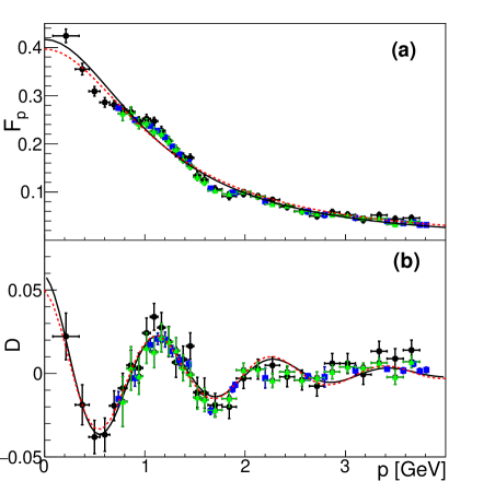
Figure 1: (a): TL proton generalized FF as a function of $p$ from the data of BaBar, Ref. Lees et al. (2013a) (black circles), BESIII-ISR Ablikim et al. (2019) (blue squares) and BESIII-SC Ablikim et al. (2020) (green triangles), with the regular background fit with Eq. (7) (black solid line ); (b): data after subtraction, fitted with Eq. (8) (black solid line). For comparison the fit from Ref. Bianconi and Tomasi-Gustafsson (2015) (red dashed lines) is also shown.

As shown in Fig. 1, even with a slightly worse normalized $\chi^{2}$, the new fit (black solid line) follows closely the one on the only BaBar data Bianconi and Tomasi-Gustafsson (2015) (red dashed line). Let us note that the consistency of the data obtained with different methods, beam scan and ISR, rules out the possibility that the oscillations could be an artefact of the ISR technique or of the photon detection.

IV Global Fit of the data

The cross section or the effective FF data can also be directly fitted with the six-parameter function $F_{p}^{\rm fit}(p)$ of Eq. (6). The parameters are reported in Table 3 and the fit is illustrated in Fig. 2 as a function of the relative momentum $p$ (black solid line), together with the result from Ref. Bianconi and Tomasi-Gustafsson (2015).

Table 3: Six-Parameters fit, Eq. (6), of the annihilation cross section $\sigma_{e^{+}e^{-}\to\bar{p}p}$ as a function of relative momentum $p$ for the BaBar, BESIII and CMD-3 data.

Ref.	$F_{0}$	$m_{a}^{2}$	$A$	$B$	$C$	$D$	$\displaystyle\frac{\chi^{2}}{\rm n.d.f.}$
		(GeV2)		(GeV-1)	(GeV-1)
Ablikim et al. (2019, 2020); Lees et al. (2013a, b); Akhmetshin et al. (2019)	9.7 $\pm$ 0.3	7.1 $\pm$ 0.5	0.073 $\pm$ 0.007	1.05 $\pm$ 0.07	5.51$\pm$ 0.09	0.04 $\pm$ 0.1	$\displaystyle\frac{278}{118-6}=2.5$

Extending the data sets does not change essentially the fit, worsening the $\chi^{2}$. The inclusion of the CMD-3 data heightens the curve in the near threshold region. The blue dash-dotted line corresponds to a constant fitted in the range $0.1<\sqrt{s}<0.9$ GeV, that gives the average value of the cross section $\bar{\sigma}=0.87\pm 0.02$ nb. Such a value is close to the cross section at the production threshold for a structureless fermions Baldini et al. (2009), as for instance that of the reaction $e^{+}e^{-}\to\mu^{+}\mu^{-}$.

Fig. 3 shows the data on the effective FF together with the curves that represent the corresponding fit functions.

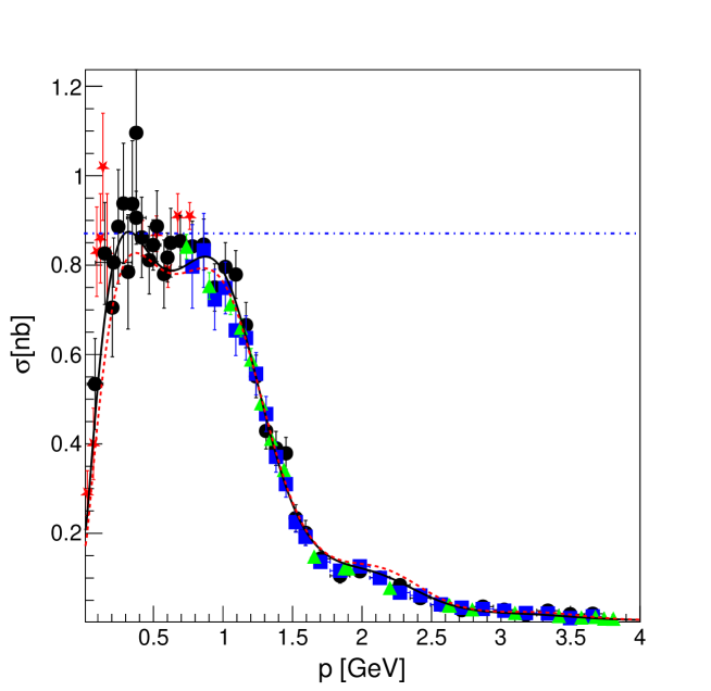
Figure 2: Born cross section for $e^{+}+e^{-}\to p+\bar{p}$ as a function of the momentum $p$. The data are from CMD-3 Akhmetshin et al. (2019) (red stars), BaBar Lees et al. (2013a, b) (black circles) BESIII-ISR Ablikim et al. (2019) (blue squares) and BESIII-SC Ablikim et al. (2020) (green triangles) are shown together with the six-parameter fit from Eqs. (6,7,8) and Table 3(black solid line), compared to the fit from Ref. Bianconi and Tomasi-Gustafsson (2015) (red dashed line). The blue dash-dotted line corresponds to a constant, fitted in the range $0.1<\sqrt{s}<0.9$ GeV.

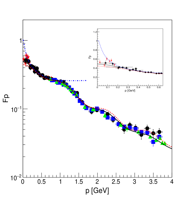
Figure 3: Same as Fig. 2 but for the TL proton generalized FF. The blue dash-dotted line is the expectation for a constant cross section $\sigma=0.87$ nb.

IV.1 Analysis of the form factor ratio $R$

The comparison between the absolute values of the electric and magnetic FFs in the TL and SL regions can be more easily done by considering their ratio. Exploiting the Akhiezer-Rekalo recoil proton polarization method Akhiezer and Rekalo (1968, 1974), that represents a unique and very powerful technique to extract directly the FF ratio $G_{E}/G_{M}$ from the longitudinal to transverse recoil proton polarization in the elastic scattering process ${\vec{e}}^{\,-}p\to e^{-}\vec{p}$, the JLab-GEP Collaboration obtained very precise values of $R$ in a wide region of transferred momenta Puckett et al. (2017, 2012). Note that the individual FFs can not be determined by this method. Therefore it is assumed that the magnetic FFs is well known from the unpolarized cross section measurements.

In the TL region, the present data from the BESIII Collaboration bring new information on the ratio of the FFs moduli with comparable precision as in the scattering region. The data from BaBar and BESIII are plotted in Fig. 4 as a function of $|q^{2}|$. The choice of this variable does allow to show on the same graph SL and TL values of the FF ratio and of their moduli respectively Tomasi-Gustafsson and Rekalo (2001).

While the SL data (red squares in Fig. 4) show a monotone decrease, the TL ones (green triangles in Fig. 4)  Ablikim et al. (2020), decrease too, but show the presence of oscillations, not contradicting the results from BaBar Lees et al. (2013a) (black circles in Fig. 4). One can see a minimum in the TL range $(5-6)$ GeV², in correspondance to a little dip in the SL region, that should be confirmed, because it lies just at the square momentum transfer corresponding to the kinematical limits of two experiments of the JLab-GEP Collaboration.

The SL and TL values of the FF ratio, move away with a smooth decrease from $1/\mu_{p}$ ($\mu_{p}$ is the proton magnetic moment in units of the Bohr magneton) at $q^{2}=0$, and from unity at the production threshold $q^{2}=4m_{p}^{2}$, respectively. These are the values expected from the definitions given above, as well as, at large transferred momenta, from the QCD quark counting rules  Matveev et al. (1973); Brodsky and Farrar (1973). This is an indication that the perturbative domain has not been reached and corroborates the predictions from Ref. Kuraev et al. (2012). Following a similar approach as for the effective FF, we fit the ratio in the TL region with a function $F_{R}$ reproducing a monopole decrease and a damped oscillation:

$$F_{R}(\omega(s))=\displaystyle\frac{1}{1+\omega^{2}/r_{0}}\left[1+r_{1}e^{-r_{2}\omega}\sin\left(r_{3}\omega\right)\right],\ \omega=\sqrt{s}-2m_{p}\,,$$ (9)

where the unitary normalization at the production threshold, $F_{R}(4m_{p}^{2})=1$, is imposed. The curve representing the fit function, Eq. (9), obtained with the parameters reported in Table 4, is shown as a black line in Fig. 4, together with the corresponding data on the TL ratio $R$ (black circles and green triangles). The monopole and the oscillatory components are also shown.

Table 4: 4-parameters fit for $R$ as a function of $q^{2}$.

$r_{0}$	$r_{1}$	$r_{2}$	$r_{3}$	$\displaystyle\frac{\chi^{2}}{\rm n.d.f}$
(GeV2)		(GeV-1)	(GeV-1)
3 $\pm$ 2	0.5 $\pm$ 0.1	1.5 $\pm$ 1.2	9.3 $\pm$ 0.5	$\displaystyle\frac{14}{22-4}=0.8$

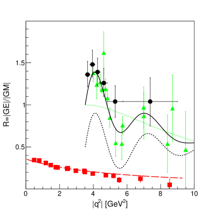
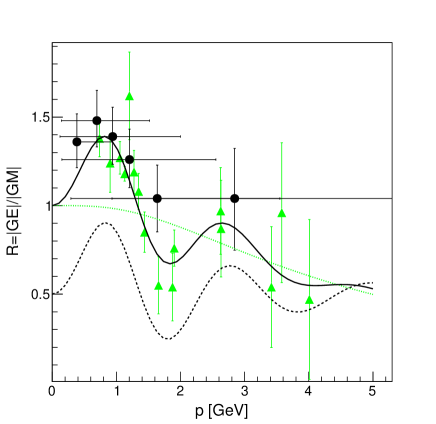
Figure 4: Ratio $R=|G_{E}|/|G_{M}|$ as a function of $|q^{2}|$ (left) and $p$ (right) from BaBar (black circles) Lees et al. (2013a, b) and BES-SC (green triangles) Ablikim et al. (2020). The solid black line is the fit from Eq. (9), decomposed in the monopole component (green dashed line) and the oscillatory component (black dotted line - shifted up by 0.5). The SL ratio from the JLab-GEp Collaboration Puckett et al. (2017) is also shown (red squares), together with its constrained monopole fit (red long-dashed line).

The red long-dashed line in Fig. 4 visualizes a one-parameter monopole function, constrained to $1/\mu_{p}$ at $q^{2}=0$. Let us remind that in the space-like region the electric FF is normalized to 1 (in unit of electric charge) and the magnetic FF is normalized to $\mu_{p}$ at $q^{2}=0$ .

In Ref. Kuraev et al. (2012) it was suggested that a faster decreasing behavior of the electric FF compared to the magnetic FF in the SL, as well as in the TL region, is expected as a consequence of the presence of an inner volume inside the nucleon that is electrically neutral (short distances corresponding to large transferred momenta). The consequence is a dipole behavior for the magnetic FF and an additional monopole decrease for the electric FF, so that the ratio decreases like a monopole.

IV.2 Zero crossing of the angular asymmetry ${\cal A}$

A further possibility to illustrate these results, knowing the ratio $R$ and the fit function, is to calculate the angular asymmetry, ${\cal A}(s)$, from Eq. (3). By definition, it assumes values in the range $[-1,1]$, being null at the production threshold, $i.e.,$ ${\cal A}(4m_{p}^{2})=0$. The data and the fit on ${\cal A}$ are shown in Fig. 5.

It has been previously pointed out that, when extracted directly from the cross section, the relative error on this variable is equivalent to an error on $R^{2}$, being therefore preferable for the extraction of the individual FFs Singh et al. (2016); Tomasi-Gustafsson and Dbeyssi (2014).

One can see that ${\cal A}(s)$ crosses zero at $s=(4.62\pm 0.07)$ GeV², meaning that, also at this squared momentum transferred, the modulus of the ratio is equal to one, and hence, $|G_{E}|=|G_{M}|$. The uncertainty is obtained by varying the function in a $\pm 5\%$ range (dashed black lines). The determination of the zero crossing gives a precise experimental constrain on FF models.

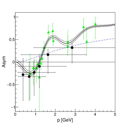
Figure 5: Angular asymmetry as a function of $|q^{2}|$ (left) and of $p$ (right) from BaBar (black circles), BESIII-SC (green triangles). The dash-dotted blue curve corresponds to a constant and unitary ratio, $i.e.,$ $|R|=1$, while the solid black curve is related to the fit function $F_{R}(s)$, with the dashed black curves representing a $\pm 5\%$ variation of the function.

IV.3 Individual form factors $|G_{E}|$ and $|G_{M}|$

The monopole background, used to fit the FF ratio is consistent with Ref. Kuraev et al. (2012) where it was suggested that the magnetic FF would follow a dipole dependence, whereas an additional monopole factor would induce a faster decrease of the electric FF in both SL and TL regions.

Overlapping the data for $|G_{E}|$ and $|G_{M}|$, extracted separately for the first time by the BESIII Collaboration Ablikim et al. (2020), from $e^{+}e^{-}\to\bar{p}p$ differential cross section data, the different behavior of the two FFs becomes visible and sizeable, as shown in Fig. 6. Surprisingly, $|G_{E}|$ and $|G_{M}|$ are also different at smaller $q^{2}$, (even though they should coincide at the production threshold) and seem to converge towards small values or to zero at large $q^{2}$.

One may inquire if the oscillations that are present in the cross section and in the effective FF are also visible in the individual FFs, and, in this case, if they have to be attributed to the electric or the magnetic FF, or to both of them. The modulus of the electric FF, $|G_{E}|$, shows larger deviations from a smooth behaviour, in particular it has a dip around 5-6 GeV², whereas $|G_{M}|$ follows closely a $(q^{2})^{-2}$ decrease. The relations between the pairs of functions ($|G_{E}|$, $|G_{M}|$) and ($R$, $F_{p}$) are:

$$|G_{E}(s)|=F_{p}(s)\sqrt{\frac{1+2\tau}{R^{2}(s)+2\tau/R^{2}(s)}}\hskip 28.45274pt|G_{M}(s)|=F_{p}(s)\sqrt{\displaystyle\frac{1+2\tau}{R^{2}(s)+2\tau}}.$$ (10)

By means of these expressions, the moduli of the electric and magnetic FFs can be calculated using for the ratio $R$ and the effective FF $F_{p}$ their fit function $F_{R}$, Eq. (9), and $F_{p}^{\rm fit}$, Eq. (6), respectively. The resulting curves are shown in Fig. 6. This procedure gives by construction a smooth description of the individual moduli of the two FFs, from threshold up to the highest experimentally accessible values of $s$ and represents a particular interest to illustrate the near threshold behavior, as the extrapolation of the FF data is constrained by the condition $R(s=4m_{p}^{2})=1$.

The result is shown in Fig. 6. Oscillations characterize both FFs, although they are more smooth on $|G_{M}|$. By the definition of the $F_{R}(s)$ fit function, the convergence of the two electric and magnetic FFs, and hence, also of the effective one, to a common value at the production threshold is implied and we find: $|G_{E}(4m_{p}^{2})|=|G_{M}(4m_{p}^{2})|=|F_{p}(4m_{p}^{2})|\equiv F_{\rm th}\simeq 0.48$.

Note that the QCD model fitted to the cross section data Tomasi-Gustafsson et al. (2005), when extrapolated back to the threshold, gives a common value for the FFs equal to $F_{\rm th}\simeq 0.34$. On the other hand, the vector meson dominance (VMD) model of Ref. Bijker and Iachello (2004) gives $F_{\rm th}\simeq 0.29$. The comparison between the data and these models is shown in Fig. 7. The QCD extrapolation provides, by definition, the same prediction for the two FFs, as it depends on the number of the quarks involved in the process. The VDM model of Ref.  Bijker and Iachello (2004) predicts a steeper behavior for $|G_{M}|$ and a number of resonances occurring in the unphysical region, i.e., the portion of the TL region lying below the production threshold. Such a region is accessible through the reaction $\bar{p}p\to e^{+}e^{-}\pi^{0}$ Adamuscin et al. (2007) and can be investigated in next future at the PANDA@FAIR facility Ritman (2005).

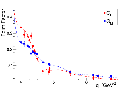
Figure 6: $|G_{E}|$ (red circles) and $|G_{M}|$ (blue squares) from BESIII. The dashed red (dash-dotted blue) line is the calculation of $|G_{E}|$ and $|G_{M}|$ from the fits of the effective FF $F_{p}$ and the ratio $R$.

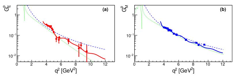
Figure 7: (a) $|G_{E}|$ (red circles) and (b) $|G_{M}|$ (blue squares) from the BESIII Collaboration. The dashed blue (solid green) curve is the calculation of $|G_{E}|$ and $|G_{M}|$ from the QCD extrapolation Tomasi-Gustafsson et al. (2005) and from the VMD model of Ref. Bijker and Iachello (2004).

V Discussion and Conclusions

We have considered the recent data on TL proton FFs from Ref. Ablikim et al. (2019, 2020); Akhmetshin et al. (2019). These data confirm the regular oscillations found in Ref. Bianconi and Tomasi-Gustafsson (2015, 2017). We present a general fit of these data, that includes and updates the previous analysis. A more precise determination of the oscillation parameters has been done. In particular the oscillation period is a relevant parameter since it has been related to sub-hadron scale processes Bianconi and Tomasi-Gustafsson (2015, 2017). A similar behavior would be shown by the future $e^{+}e^{-}\to n\bar{n}$ data S.Ahmed (2020), in this case the oscillation parameters should bring information on the dynamics underlying the formation from the vacuum of quark-diquark states, the quark having different flavor.

Our analysis does confirm a faster average decrease of the electric FF compared to the magnetic one, following a similar behavior as in the SL region. It is in agreement with the predictions of Ref. Kuraev et al. (2012), where such a decreasing behavior was attributed to the existence of an electrically neutral inner region in the proton. It is also compatible with the VMD model of Ref. Bijker and Iachello (2004), that slightly overestimates the magnetic FF. This appears also from the fact that the QCD behavior, that does not differentiate the two FFs, overestimates $G_{E}$, reproducing better $G_{M}$.

The new proton data, together with the future neutron data, will require a revision of the phenomenological models based on fitting procedures, as the parameters were determined in TL region, from the effective FF only. This will be the object of a future work.

VI Appendix: expressions of the fit functions

The change of variables $s=s(p)$, as well as $p=p(s)$, follows from the relations

$$s=2m_{p}\left(m_{p}+\sqrt{p^{2}+m_{p}^{2}}\right)\,,\hskip 28.45274ptp=\sqrt{s\left(\frac{s}{4m_{p}^{2}}-1\right)}\,.$$ (11)

Therefore Eqs. (7,8) can be rewritten as:

$$F_{\rm 3p}(s) = \frac{F_{0}}{\left(1+\frac{s}{m_{a}^{2}}\right)\left(1-\frac{s}{m_{0}^{2}}\right)^{2}}=$$ (12)

$$= \frac{F_{0}}{\left(1+\frac{2m_{p}\left(m_{p}+\sqrt{p^{2}+m_{p}^{2}}\right)}{m_{a}^{2}}\right)\left(1-\frac{2m_{p}\left(m_{p}+\sqrt{p^{2}+m_{p}^{2}}\right)}{m_{0}^{2}}\right)^{2}}\,,$$

$$F_{\rm osc}(p(s)) = Ae^{-B\sqrt{s\left(\frac{s}{4m_{p}^{2}}-1\right)}}\cos\left[C\sqrt{s\left(\frac{s}{4m_{p}^{2}}-1\right)}+D\right]=Ae^{-Bp}\cos(Cp+D)\,.$$ (13)

Equation (9) can be expressed as a function of $s$ as

$$F_{R}(\omega(s))=\displaystyle\frac{1}{1+(\sqrt{s}-2m_{p})^{2}/r_{0}}\left[1+r_{1}e^{-r_{2}\left(\sqrt{s}-2m_{p}\right)}\sin\left(r_{3}\left(\sqrt{s}-2m_{p}\right)\right)\right]\,,$$ (14)

taking into account that $\omega=\sqrt{s}-2m_{p}$.

References

- Pacetti et al. (2015) S. Pacetti, R. Baldini Ferroli, and E. Tomasi-Gustafsson, Phys. Rept. 550-551, 1 (2015).
- Baier et al. (1973) V. N. Baier, V. S. Fadin, and V. A. Khoze, Nucl. Phys. B65, 381 (1973).
- Lees et al. (2013a) J. Lees et al. (BaBar Collaboration), Phys. Rev. D87, 092005 (2013a).
- Ablikim et al. (2019) M. Ablikim et al. (BESIII), Phys. Rev. D99, 092002 (2019), eprint 1902.00665.
- Lees et al. (2013b) J. Lees et al. (BaBar Collaboration), Phys. Rev. D88, 072009 (2013b).
- Ablikim et al. (2020) M. Ablikim et al. (BESIII), Phys. Rev. Lett. 124, 042001 (2020), eprint 1905.09001.
- Puckett et al. (2017) A. J. R. Puckett et al., Phys. Rev. C96, 055203 (2017), [erratum: Phys. Rev.C98,no.1,019907(2018)], eprint 1707.08587.
- Puckett et al. (2012) A. Puckett et al., Phys. Rev. C 85, 045203 (2012), eprint 1102.5737.
- Zichichi et al. (1962) A. Zichichi, S. Berman, N. Cabibbo, and R. Gatto, Nuovo Cim. 24, 170 (1962).
- Dubnickova et al. (1996) A. Dubnickova, S. Dubnicka, and M. Rekalo, Nuovo Cim. A 109, 241 (1996).
- Akhmetshin et al. (2019) R. R. Akhmetshin et al. (CMD-3), Phys. Lett. B794, 64 (2019), eprint 1808.00145.
- Bianconi and Tomasi-Gustafsson (2015) A. Bianconi and E. Tomasi-Gustafsson, Phys. Rev. Lett. 114, 232301 (2015).
- Jones et al. (2000) M. Jones et al. (Jefferson Lab Hall A), Phys. Rev. Lett. 84, 1398 (2000), eprint nucl-ex/9910005.
- Tomasi-Gustafsson and Rekalo (2001) E. Tomasi-Gustafsson and M. Rekalo, Phys. Lett. B 504, 291 (2001).
- Kuraev et al. (2012) E. Kuraev, E. Tomasi-Gustafsson, and A. Dbeyssi, Phys. Lett. B712, 240 (2012).
- Tomasi-Gustafsson et al. (2005) E. Tomasi-Gustafsson, F. Lacroix, C. Duterte, and G. Gakh, Eur. Phys. J. A 24, 419 (2005), eprint nucl-th/0503001.
- Belushkin et al. (2007) M. Belushkin, H.-W. Hammer, and U.-G. Meissner, Phys. Rev. C 75, 035202 (2007), eprint hep-ph/0608337.
- Bijker and Iachello (2004) R. Bijker and F. Iachello, Phys. Rev. C69, 068201 (2004).
- Lomon and Pacetti (2012) E. L. Lomon and S. Pacetti, Phys. Rev. D 85, 113004 (2012), [Erratum: Phys.Rev.D 86, 039901 (2012)], eprint 1201.6126.
- Denig and Salme (2013) A. Denig and G. Salme, Prog. Part. Nucl. Phys. 68, 113 (2013), eprint 1210.4689.
- Bonneau and Martin (1971) G. Bonneau and F. Martin, Nucl. Phys. B27, 381 (1971).
- Benayoun et al. (1999) M. Benayoun, S. I. Eidelman, V. N. Ivanchenko, and Z. K. Silagadze, Mod. Phys. Lett. A14, 2605 (1999), [Frascati Phys. Ser.15(1999)], eprint hep-ph/9910523.
- Bytev et al. (2011) V. V. Bytev, E. A. Kuraev, E. Tomasi-Gustafsson, and S. Pacetti, Phys. Rev. D84, 017301 (2011), eprint 1103.4470.
- Hoang (1996) A. H. Hoang, in Electroweak interactions and unified theories. Proceedings, 31st Rencontres de Moriond, Leptonic Session, Les Arcs, France, March 16-23, 1996 (1996), pp. 129–134, eprint hep-ph/9606288.
- Gakh and Tomasi-Gustafsson (2005) G. Gakh and E. Tomasi-Gustafsson, Nucl. Phys. A 761, 120 (2005), eprint nucl-th/0504021.
- Akhmetshin et al. (2016) R. Akhmetshin et al. (CMD-3), Phys. Lett. B 759, 634 (2016), eprint 1507.08013.
- Baldini et al. (2009) R. Baldini, S. Pacetti, A. Zallo, and A. Zichichi, Eur. Phys. J. A 39, 315 (2009), eprint 0711.1725.
- Akhiezer and Rekalo (1968) A. Akhiezer and M. Rekalo, Sov. Phys. Dokl. 13, 572 (1968).
- Akhiezer and Rekalo (1974) A. Akhiezer and M. Rekalo, Sov. J. Part. Nucl. 4, 277 (1974).
- Matveev et al. (1973) V. Matveev, R. Muradyan, and A. Tavkhelidze, Teor. Mat. Fiz. 15, 332 (1973).
- Brodsky and Farrar (1973) S. J. Brodsky and G. R. Farrar, Phys. Rev. Lett. 31, 1153 (1973).
- Singh et al. (2016) B. Singh et al. (PANDA), Eur. Phys. J. A 52, 325 (2016), eprint 1606.01118.
- Tomasi-Gustafsson and Dbeyssi (2014) E. Tomasi-Gustafsson and A. Dbeyssi (PANDA), EPJ Web Conf. 66, 06024 (2014).
- Adamuscin et al. (2007) C. Adamuscin, E. Kuraev, E. Tomasi-Gustafsson, and F. Maas, Phys. Rev. C 75, 045205 (2007), eprint hep-ph/0610429.
- Ritman (2005) J. Ritman (PANDA), Int. J. Mod. Phys. A 20, 567 (2005).
- Bianconi and Tomasi-Gustafsson (2017) A. Bianconi and E. Tomasi-Gustafsson, Phys. Rev. C 95, 015204 (2017), eprint 1611.02149.
- S.Ahmed (2020) S.Ahmed (BESIII), in 3th European Research Conference on Electromagnetic Interactions with Nucleons and Nuclei, 27/10 – 02/11 2019,Paphos, Cyprus (2020).