EMCCD for Pyramid wavefront sensor: laboratory characterization

Abstract

Electro-Multiplying CCDs offer a unique combination of speed, sub-electron noise and quantum efficiency. These features make them extremely attractive for astronomical adaptive optics. The SOUL project selected the Ocam2k from FLI as camera upgrade for the pyramid wavefront sensor of the LBT SCAO systems. Here we present results from the laboratory characterization of the 3 of the custom Ocam2k cameras for the SOUL project. The cameras showed very good noise ($0.4e^{-}$ and $0.4-0.7e^{-}$ for binned modes) and dark current values ($1.5e^{-}$). We measured the camera gain and identified the dependency on power cycle and frame rate. Finally, we estimated the impact of these gain variation in the SOUL adaptive optics system. The impact on the SOUL performance resulted to be negligible.

1 INTRODUCTION

Wavefront sensors for astronomical adaptive optics require fast and low noise cameras with hundreds by hundreds of pixels. Following these requirements, in the last 10 years, the top class telescopes started to use a new class of CCDs, the Electron-multiplying CCD. These new devices have been introduced in AO systems[1, 2, 3] with Shack Hartmann[4] and Pyramid WaverFront Sensors[5] (PWFS).

Ocam2k by First Light Advanced Imagery [6, 7] (FLI) is an EMCCD with sub-electron read out noise, implementing the CCD220 by e2v [8, 9].

The aim of this paper is to present the results of the laboratory characterization of 3 of the 5 Ocam2k cameras that will be implemented on the PWFS of the Single conjugated adaptive Optics Upgrade for LBT (SOUL) [10]. In fact, the SOUL project will upgrade the four existing SCAO systems of LBT [11, 12], and Ocam2k has been selected to replace the Little Joe CCD39 camera by SciMeasure [13] currently operating at LBT.

FLI customized these Ocam2k cameras to match SOUL specifications: the mechanical layout has been expressly designed for the implementation on the FLAO WFS and 2 extra read-out modes added (on-chip binning mode 3x3 and 4x4).

Ocam2k camera has a negligible RON and larger format with respect to Little Joe CCD39: this allows to improve contrast on bright magnitude guide star thanks to an higher sampling of the pupil and to push the limiting magnitude of about 2 magnitudes thanks to the lower measurement noise. Finally, the turbulence and telescope vibration will be rejected with higher efficiency thanks to the higher frame rate [10].

2 Analysis of dark frames

In this section, we describe the results obtained analyzing frames without light (metallic screw cap on). These measurements are used to compute Read-Out Noise, Dark Current and to evaluate Bias stability. Note that, we consider the value for the on-chip multiplication gain as set on the camera interface and the nominal one for the CCD gain ($g=1/30$), for all pixels. We acquired 1 set of 5999 frames (the buffer size of the frame-grabber) for each combination of the following parameters:

• Acquisition mode = 1 (full frame), 2 (crop), 3 (binning 2x2), 4 (binning 3x3) and 5 (binning 4x4)

• Frame rates = 100, 200, 300, 500, 1000, 1500, 2060Hz

• On chip multiplication gain $m=1$ and $m=600$.

We repeated these acquisitions after few hours and a full power cycle of the camera for a total of 156 sets.

2.1 Read-Out Noise

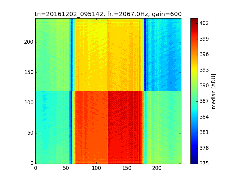
(a) Average dark frame at 2067 fps (6000 frames).

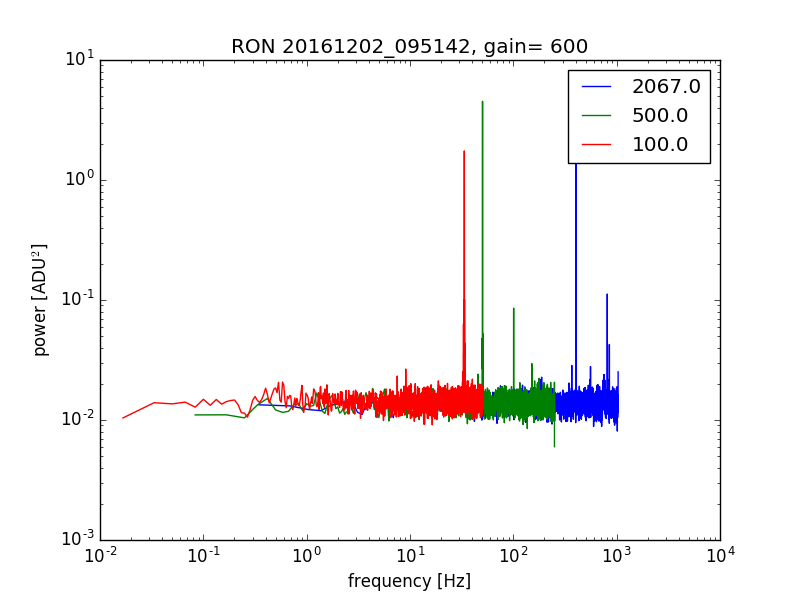
(b) Counts Power Spectral Density for different frame rate speeds. Dark frames..

Figure 1: Output of dark frames analysis.

An example of dark frame is reported in Figure 1(a). The noise does not present the typical white spatial distribution due to the ADC read-out. High spatial frequency patterns are present over the entire frame. The averaged temporal spectrum presents clear structures too as can see in Figure 1(b).

Read-Out Noise (RON), is estimated pixel by pixel from the temporal standard deviation at the maximum frame rate, $f_{MAX}$:

$$R_{e}=\sigma(f_{MAX})=\sqrt{\frac{\sum_{i=1}^{N}(p_{i}-\mathrm{bar}{p})^{2}}{N}}$$ (1)

where $p_{i}$ is the pixel value expressed in $e^{-}=\frac{c_{i}}{mg}$, $c_{i}$ are the pixel counts, $m$ is the on-chip multiplication gain, $g$ is the CCD gain expressed in $ADU/e^{-}$, $\mathrm{bar}{p}$ is the average pixel counts value, $i$ is the frames index and $N=5999$.
We measured $R_{e}$ in with on-chip multiplication gain $m=600$. The results are summarized in Table 1. Notice that, as said before, in this analysis, we considered the value of $m$ as set in the camera interface (600) and the nominal one for the CCD gain (g = 0.03$ADU/e^{-}$), for all pixels. The obtained values of noise are in good agreement with the ones provided by e2v and FLI, as can be seen in Table 1. As expected by FLI, the on-chip binning slightly increases the RON.

All the measured values are compliant with the specifications: RON$<0.5e^{-}$ with $m=600$ without binning and RON$<1e^{-}$ with $m=600$ for binned modes.

Table 1: Read-Out noise for the three cameras. Third row reports the values given by e2v for m= 1000. Fourth and fifth rows are the values from First Light for binning 1x1 and 2x2 respectively. The values in the test in Arcetri labs are shown in the last 4 rows.

	Binning		$R_{e}$ [e-]
Camera no.		39	40	41
e2v (m=1000, 1274fps)		0.295	0.332	0.347
First Light (m=600, 2000fps)	bin 1x1	0.384	0.344	0.344
	bin 2x2	0.520	0.431	0.479
OAA (m=600, 2066fps)	bin 1x1	0.372	0.343	0.339
OAA (m=600, 3620fps)	bin 2x2	0.489	0.424	0.465
OAA (m=600, 4890fps)	bin 3x3	0.633	0.605	0.556
OAA (m=600, 5900fps)	bin 4x4	0.739	0.671	0.668

2.2 Dark Current

Dark Current, $D_{e}$, is estimated from the linear relationship between integration time and temporal variance:

$$\sigma^{2}_{T}=D_{e}T+\sigma^{2}_{T}(f=\infty)$$ (2)

where $T$ is the integration time, $\sigma^{2}_{T}(f=\infty)$ is the count variance on the pixel corresponding to $T$, and $\sigma^{2}_{T}(f=\infty)\simeq R^{2}_{e}$. Dark current results are shown in Table 2. As for the RON we considered the nominal values $m=600$ and $g=1/30$, for all pixels. The estimated values are in good agreement with the ones provided by FLI.

Table 2: Dark current for the three cameras. First and second rows report the values given by e2v (m = 1000) and First Light (m = 600) respectively. The values from our estimation (from binning 3x3 and 4x4 data) is shown in the last row. Notice that we considered an on-chip multiplication gain of 600 for every pixel.

		$D_{e}$ [e-/pixel/s]
Camera no.	39	40	41
e2v (m=1000, 1274fps)	5.10	6.37	5.10
First Light (m=600, 2000fps)	2.56	3.58	3.10
OAA (m=600)	2.16	2.80	2.58

3 Analysis of illuminated frames

In this section we describe the measurements made with light and the following data analysis. These measurements are used to compute the on-chip multiplication gain and electronic gain of the CCD. These measurements are then used to obtain a more accurate estimation of RON and dark current. Moreover, the spatial distribution of the gain will be used to evaluate the need of a flat field correction.

3.1 Detector gain

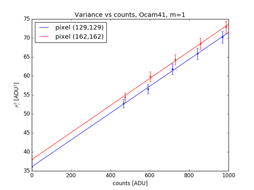
(a) Variance vs counts for two pixels, $m=1$. Curves are the best fits (equation 3)

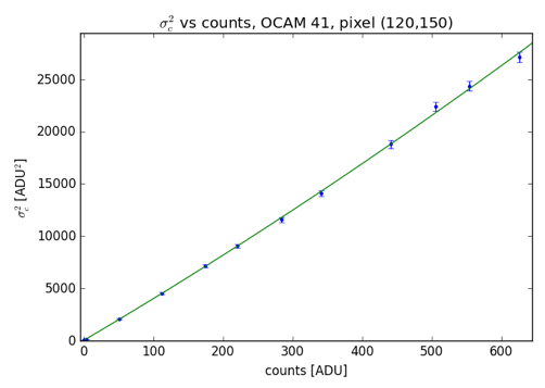
(b) Variance vs counts for one pixel, $m=600$.

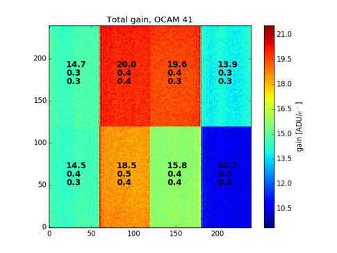
(c) Total gain $G$ estimated as the linear component of equation 3. For each sector the three numbers are: the average value over the sector, the standard deviation and the average fitting error.

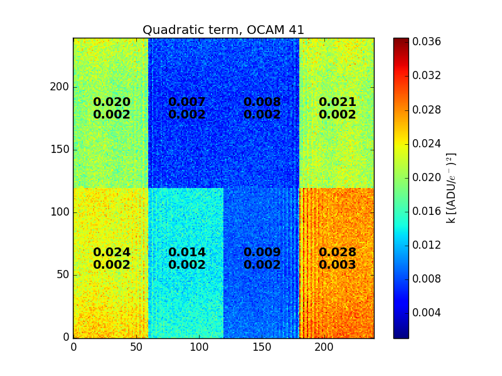
(d) Quadratic term $k$ of equation 3. For each sector the two numbers are: average value over the sector and standard deviation of the quadratic part of the total gain.

Figure 2: Typical output of the data analysis for camera no. 41.

Table 3: Gains for camera no. 41 with $m=600$ and all modes. $k$ is the quadratic term and $G=m*g$ is the total gain in ADU$/e^{-}$.

	Bin 1		Crop		Bin 2		Bin 3		Bin 4
Sector	$k$	$G[\frac{ADU}{e^{-}}]$	$k$	$G[\frac{ADU}{e^{-}}]$	$k$	$G[\frac{ADU}{e^{-}}]$	$k$	$G[\frac{ADU}{e^{-}}]$	$k$	$G[\frac{ADU}{e^{-}}]$
0	0.013	16.8	-	-	0.014	23.5	0.015	25.8	0.010	28.3
1	0.004	21.5	0.005	21.4	0.004	28.3	0.001	31.6	0.000	32.9
2	0.004	17.6	0.004	17.7	0.003	25.4	0.000	29.4	0.010	30.6
3	0.014	13.4	-	-	0.016	18.4	0.016	22.0	0.002	24.8
4	0.012	15.0	-	-	0.011	19.6	0.006	21.0	0.000	22.7
5	0.003	19.7	0.004	19.7	0.002	24.9	0.000	25.2	0.000	25.5
6	0.003	20.3	0.003	20.3	0.002	25.6	0.000	26.8	0.000	27.2
7	0.014	14.8	-	-	0.014	19.3	0.012	20.7	0.008	22.6

Table 4: Gains for the three cameras in binning 1x1 mode. $g$ is the electronic gain in ADU$/e^{-}$ (measured with $m=1$), $k$ is the quadratic term and $G=m*g$ is the total gain in ADU$/e^{-}$.

	no. 39, Bin1			no. 40, Bin1			no. 41, Bin1
Sector	$g[\frac{ADU}{e^{-}}]$	$k$	$G[\frac{ADU}{e^{-}}]$	$g[\frac{ADU}{e^{-}}]$	$k$	$G[\frac{ADU}{e^{-}}]$	$g[\frac{ADU}{e^{-}}]$	$k$	$G[\frac{ADU}{e^{-}}]$
0	0.036	0.007	17.2	0.039	0.006	19.3	0.035	0.013	16.8
1	0.036	0.000	21.0	0.038	0.002	20.9	0.036	0.004	21.5
2	0.032	0.000	19.6	0.036	0.002	20.9	0.030	0.004	17.6
3	0.035	0.005	16.9	0.039	0.009	17.7	0.030	0.014	13.4
4	0.033	0.003	23.7	0.038	0.006	16.9	0.036	0.012	15.0
5	0.032	0.000	24.6	0.036	0.002	18.5	0.036	0.003	19.7
6	0.035	0.000	24.1	0.038	0.002	21.7	0.036	0.003	20.3
7	0.036	0.002	24.4	0.039	0.009	18.2	0.036	0.014	14.8

We present here the measurements and analysis done to compute on-chip multiplication gain and electronic gain of the CCD. At a given detector configuration, the fluctuation in time (frame by frame) of the pixel value is the sum of the Read Out Noise, $R_{e}$, and the photon noise, $\sigma_{e}^{2}$. Since the random arrival rate of photons controls the photon noise and the photon noise obeys the laws of Poissonian statistics we obtain:

$$\sigma^{2}_{c}=R_{c}^{2}+\frac{G}{F}c+kc^{2}$$ (3)

where $\sigma^{2}_{c}$ is the counts variance, $R_{c}=GR_{e}$ is Read Out Noise in square counts, $c$ are the counts, $G=m*g$ is the total gain, $k$ is an additional term to take into account possible non-linearities and $F$ is the excess noise factor due to the electronic multiplication. We considered $F=1$ for $m=1$ and $F=2$ for $m=600$. Hence, without the electronic multiplication ($m=1$, $F=1$), and neglecting the non-linear term ($k<<10^{-3}$ for $m=1$), we obtain:

$$\sigma^{2}_{c}=R_{c}^{2}+gc$$ (4)

We used an integrating sphere in order to acquire camera frames while the chip was illuminated uniformly. We used two different illumination fluxes and, for each one, we changed the integration time from the minimum up to 1ms. For each configuration (flux, $T$ and $g$) we acquire  6000 frames. We plot the counts variance versus the average counts and we fit the data with equation 3 and 4 for frames with m=600 and m=1 respectively. The error on the variance ($\delta_{\sigma^{2}}$) is computed as:

$$\delta_{\sigma^{2}}=\sqrt{\frac{1}{n}\left(\mu_{4}-\frac{n-3}{n-1}\mu_{2}^{2}\right)}$$ (5)

$$\mu_{k}=\frac{1}{n-1}\sum_{i=1}^{n}(x_{i}-\mathrm{bar}{x})^{k}$$ (6)

where $\mu_{k}$ is the $k$-th central moment, $x_{i}$ is the $i$-th value and $\mathrm{bar}{x}$ is the mean on the events. The additional term $kc^{2}$ introduces nonlinear behavior when $m>1$. The nonlinear term follow approximatively a quadratic trend respect to the average counts, as will be detailed in this section.
Figure 2 reports the typical output of the data analysis for camera no. 41. The figures refer to data in mode 1 (binning 1x1), with multiplication $m$ = 1 (Figure 2(a)) and $m$ = 600 (Figure 2(b), 2(c) and 2(d)).
According with the specification from First Light the electronic gain of the CCD should be $g=0.03$ADU$/e^{-}$ and with $m$ = 600, we have $G=m*g=$ 20 ADU/$e^{-}$ . The values measured in the central part of the CCD (quadrants 1, 2, 5, 6) are in good agreement with the expected value and the quadratic term is negligible (Figure 2). In the external part of the CCD (quadrants 0, 3, 4, 7) the quadratic term is more relevant and the total gain is depressed. Camera no. 41 measurements show bigger quadratic terms respect to the other two cameras (see Table 4).
Table 3 reports the results of the analysis on camera no. 41 with multiplication set to 600.
We can notice that the total gain becomes bigger rising the binning (see Section 3.2 to further considerations), and highest values of the total gain are associated to the lowest quadratic terms (see the results for camera n.41 in Table 4).

3.2 Read-Out Noise and Dark current with measured gains

Read-Out Noise and Dark current values shown in the previous section are computed using nominal values for $g$ and $G$. We recomputed RON and dark estimates (section 2), using the measured values of $g$ and $G$ found in section 3.1. In Table 3 we see that the $G$ values has a positive trend with the binning, reaching at bin 4 a $+25\div 50\%$ of its value at bin 1. Considering this effect, the RON results reduced for binned modes ($<0.5e^{-}$ at all binning) and the estimation of $D_{e}$ is consistent at all binning. As example, in Table 5 we report for camera n.41 the comparison for $R_{e}$ and $D_{e}$ between values obtained with nominal and measured $g$ and $G$.

Table 5: RON and dark current for camera no. 41 computed using measured gains from Table 3. Dark current values always refer to physical pixel (not binned one).

	$R_{e}$ [e-]		$D_{e}$ [e-/pixel/s]
Camera no.	41
gain value	nominal	measured	nominal	measured
bin1x1	0.34	0.40	1.16	1.46
bin2x2	0.47	0.38	2.18	1.60
bin3x3	0.56	0.45	2.43	1.47
bin4x4	0.67	0.51	2.58	1.38

4 Gain uniformity

Detector gain is a key aspect for PWFS because, in order to make a correct measurements, it requires a spatially uniform response on the chip regions where the pupil images lie. In fact, PWFS slopes calculation is done comparing the amount of light in the four pupil images[5]: different gains in the regions where the pupils light fall yields to an error on the flux measurement, propagating it in the slope estimation.

As can be seen in Figure 2(c) (and Figure 3(b) blue line, Table 3 and 4), Ocam2k gain $G$, when EM multiplication is enabled, varies manly sector by sector in the range $\pm 25\%$. Hence, flat fielding is required to work properly with PWFS and, in this section, we present our analysis on the stability of the camera gains needed to set up a correct procedure to calibrate and manage this flat fielding. Flat field measurement has been performed using an integrating sphere in order to provide uniform illumination on the chip. In the following part of this section we will only refer to the four central sectors of the chip, because the PWFS of the SOUL project has pupils which lie on a region of interest of 120$\times$120pixels.

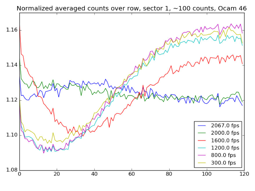
(a) Average counts on the rows with uniform illumination ($\sim$100counts) over half the 120$\times$120 central sub-frame. The values are normalized by the average on the sector. Different colors represent different frame rates.

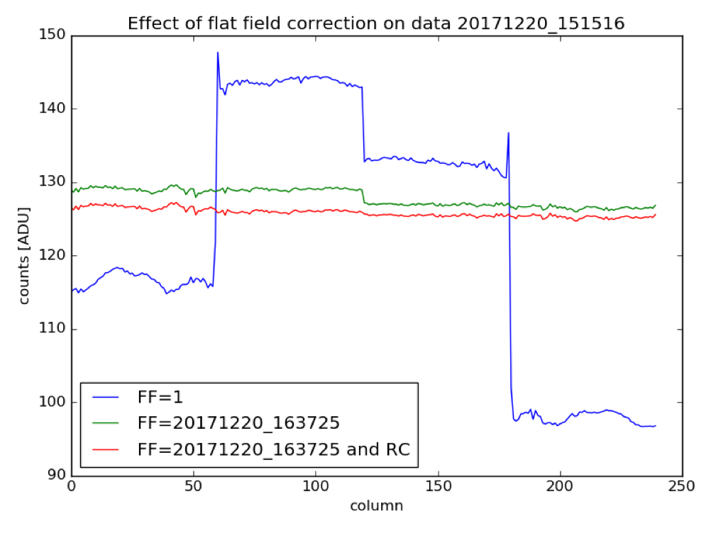
(b) Average counts over the rows for the sectors in the bottom part of the chip (from 0 to 3). Blue line is wit no flat fielding, green line flat fielding with a previous power cycle and red line is flat fielding from a previous power cycle with the sector by sector re-normalization.

Figure 3: Flat field analysis.

We will focus on two main dependencies of the flat field found during laboratory analysis: camera power cycle and integration time. After a power cycle of the camera, the average $G$ value typically changes sector by sector of few percents (see green line of Figure 3(b)). This effect can be compensated by measuring the mean $G$ value for each sector, at each power cycle, and then re-normalizing the flat field sector by sector with the obtained values. The mean $G$ value can be measured averaging the ratio between mean counts and time variance when some illumination is present. Using this procedure we need a light source stable during data acquisition (few seconds) without any requirements of spatial uniformity. Applying this method, the variation between sectors goes below 1% (see red line of Figure 3(b)). The second feature we are reporting here is the gain change row by row as function of the frame rate. In Figure 3(a) we report the counts averaged over the rows (with spatially uniform illumination) at different frame rates when both the flat field (acquired at maximum frame rate) and the sector by sector correction are applied. In the frame rate range 300-2000Hz, the maximum variation of the gain across the frame has a peak-to-valley $<10\%$. A similar behavior is already described in literature (section 4 of Dowing et al.[15]). This effect can be mitigated measuring and applying different flat fields for different frame rates reducing the gain variation to a few $\%$.

4.1 Impact of gain non uniformity on SOUL performances

This section is aimed to quantify the impact of the camera gain features described in the previous section, hypothesizing to not update flat field in case of framerate variations and camera power cycles. This estimation has been carried on using PASSATA[16], the end-to-end simulator used for all numerical simulations in the SOUL project. We run full adaptive optics end-to-end simulations of the SOUL system, using different detector gain maps, emulating the effects described in sect. 4. Simulating the SOUL system, we considered an OCam2k sub-frame of 120 x 120 pixels over the 4 central sectors. The AO system calibration (interaction matrix corrector-WFS) is simulated applying a flat detector gain map. Then the AO simulations are run using the following gain maps:

1. reference case: perfect flat field, all normalized gains are 1;

2. power cycle effect: 3 sectors gain value 1, fourth sector with gain 1.1;

3. frame rate effect: we used real averaged frames acquired at 1200Hz normalized with a flat field acquired at 2000Hz.

Table 6: Simulation parameters.

atmosphere	seeing	0.8arcsec
	$L_{0}$	40m
	aver. wind speed	16m/s
$1^{st}$ configuration	R magnitude	8	$2^{nd}$ configuration	R magnitude	13.5
	mod. amplitude	$\pm 3\lambda/D$		mod. amplitude	$\pm 4\lambda/D$
	sampl. freq.	1500Hz		sampl. freq.	300Hz
	corr. modes	630		corr. modes	299
	total time	10s		total time	16s

We simulated standard seeing conditions at LBT ($0.8$arcsec) and two cases of natural guide star: bright end (R=8, 630 corrected modes) and medium-faint (R=13.5, 299 corrected modes); more simulation parameters are reported in Table 6. In Table 7 we summarize the simulation results in terms of total wavefront residual for the considered cases. In the two right columns of the table we can see the residual wavefront difference for cases B and C with respect to the reference case, including or not the tip-tilt. These numbers show, as expected, that case B introduces mainly a static tilt, with negligible effects on higher modes. The amount of introduced tilt depends on the reference star flux. About case C, it affects a wide range of modes but with negligible impact on the overall system performances.

Table 7: Simulation results.

Case	conf.	res. RMS [nm]	diff. [nm]	diff. w/o TT [nm]
A	$1^{st}$	87.1	-	-
B	$1^{st}$	95.9	40.1	4.0
C	$1^{st}$	87.2	3.8	3.8
A	$2^{nd}$	179.0	-	-
B	$2^{nd}$	192.2	70.0	8.8
C	$2^{nd}$	182.5	35.4	31.8

Hence, we can conclude that:

• the power cycle effect (case B) introduces a static tilt of the order of $100$nm RMS, translating into an indetermination of the scientific PSF position of about 10mas; compensating with sector gain corrections, as mentioned in 4, we expect to reduce this effect down to the order of a few mas;

• the frame rate effect has already a negligible impact in terms of Strehl ratio in NIR bands; using a set 3-4 flat fields, calibrated at different camera frame rates, this effect can be easily further reduced for high contrast applications.

5 Conclusion

Our laboratory measurements show that the 3 considered Ocam2k cameras are compliant with their specifications in terms of RON (about 0.4e- and 0.4-0.7e- for binned modes) and dark current (1.5e-/pixel/s). We estimated, pixel by pixel, the camera gain ($g$) and the multiplication gain ($m$) obtaining values close to the nominal ones but showing differences sector by sector. The 4 internal sectors of the chip show better values for $g$ and $G=g*m$, and a more linear behavior of the relation counts vs. time variance of counts. We found that the camera gain varies with power cycles and frame rate. Via numerical simulations we quantified the impact of these variations on the adaptive optics performances. The power cycle changes the gain sector by sector and, in the SOUL case, this translates into a global static tilt of about 10mas that can even be mitigated with an initial measurement of the sector gains. On the other side, the gain variation associated to frame rate change has a minimal impact on the performances.

The measurements and the simulations we performed do not show any major issue for the use of Ocam2k for high order PWFSs when pupil images are allocated one per chip sector, as in the SOUL case. In the case of ELTs (PWFS for GMT[17] and EELT[18, 19]), the pupil images will not fit into a single 60x120 pixel sector and the impact of the gain variations will be higher. Of course, each ELT case deserves dedicated numerical simulations; however, from the described experience with SOUL simulation and cameras, we are inclined to think that the gain effect can be efficiently mitigated with dedicated calibrations, allowing the use of Ocam2k even for the ELT PWFSs.

References

- [1] Fusco, T., Sauvage, J.-F., Mouillet, D., Costille, A., Petit, C., Beuzit, J.-L., Dohlen, K., Milli, J., Girard, J., Kasper, M.and Vigan, A., Suarez, M., Soenke, C., Downing, M., N’Diaye, M., Baudoz, P., Sevin, A., Baruffolo, A., Schmid, H.-M., Salasnich, B., Hugot, E., and Hubin, N., “Saxo, the sphere extreme ao system: on-sky final performance and future improvements,” (2016).
- [2] El Hadi, K., Fusco, T., Sauvage, J.-F., and Neichel, B., “High speed and high precision pyramid wavefront sensor: In labs validation and preparation to on sky demonstration,” in [Adaptive Optics Systems IV ], Proc.SPIE 9148, 91485C (July 2014).
- [3] Bello, D., Boucher, L., Rosado, M., Castro López, J., and Feautrier, P., “Characterization of the main components of the gtcao system: 373 actuators dm and ocam2 camera.,” (2013).
- [4] Hartmann, J., “Bemerkungen uber den Bau und die Justierung von Spektrographen,” Naturwissenschaften 20, 17–27 (1900).
- [5] Ragazzoni, R., “Pupil plane wavefront sensing with an oscillating prism,” Journal of Modern Optics 43, 289–293 (1996).
- [6] Feautrier, P., Gach, J.-L., Balard, P., Guillaume, C., Downing, M., Hubin, N., Stadler, E., Magnard, Y., Skegg, M., Robbins, M., Denney, S., Suske, W., Jorden, P., Wheeler, P., Pool, P., Bell, R., Burt, D., Davies, I., Reyes, J., Meyer, M., Baade, D., Kasper, M., Arsenault, R., Fusco, T., and Diaz Garcia, J. J., “OCam with CCD220, the Fastest and Most Sensitive Camera to Date for AO Wavefront Sensing,” PASP 123, 263 (Mar. 2011).
- [7] Feautrier, P. and Gach, J.-L., “Visible and infrared wavefront sensing detectors review in europe – part i,” (2013).
- [8] Feautrier, P., Gach, J.-L., Balard, P., Guillaume, C., Downing, M., Stadler, E., Magnard, Y., Denney, S., Wolfgang Suske, W., Jorden, P., Wheeler, P., Skegg, M., Pool, P., Bell, R., Burt, D., Reyes, J., Meyer, M., Hubin, N., Baade, D., Kasper, M., Arsenault, R., Fusco, T., and Diaz Garcia, J. J., “The l3vision ccd220 with its ocam test camera for ao applications in europe,” (2008).
- [9] Downing, M., Hubin, N., Kasper, M., Jorden, P., Pool, P., Denney, S., Suske, W., Burt, D., Wheeler, P., Hadfield, K., Feautrier, P., Gach, J.-L., Reyes, J., Meyer, M., Baade, D., Balard, P., Guillaume, C., Stadler, E., Boissin, O., Fusco, T., and Diaz, J. J., “A Dedicated L3Vision CCD for Adaptive Optics Applications,” in [Astrophysics and Space Science Library ], Beletic, J. E., Beletic, J. W., and Amico, P., eds., Astrophysics and Space Science Library 336, 321 (Mar. 2006).
- [10] Pinna, E., Esposito, S., Hinz, P., Agapito, G., Bonaglia, M., Puglisi, A., Xompero, M., Riccardi, A., Briguglio, R., Arcidiacono, C., Carbonaro, L., Fini, L., Montoya, M., and Durney, O., “SOUL: the single conjugated adaptive optics upgrade for LBT,” Proc. SPIE 9909, 9909 – 9909 – 10 (2016).
- [11] Hill, J. M., “The Large Binocular Telescope,” Appl. Opt. 49, 115–122 (Apr. 2010).
- [12] Esposito, S., Riccardi, A., Pinna, E., Puglisi, A., Quirós-Pacheco, F., Arcidiacono, C., Xompero, M., Briguglio, R., Agapito, G., Busoni, L., Fini, L., Argomedo, J., Gherardi, A., Brusa, G., Miller, D., Guerra, J. C., Stefanini, P., and Salinari, P., “Large Binocular Telescope Adaptive Optics System: new achievements and perspectives in adaptive optics,” in [Astronomical Adaptive Optics Systems and Applications IV ], Proc. SPIE 8149 (Sept. 2011).
- [13] DuVarney, R. C., Bleau, C. A., Motter, G. T., Shaklan, S. B., Kuhnert, A. C., Brack, G., Palmer, D., Troy, M., Kieu, T., and Dekany, R. G., “EEV CCD39 wavefront sensor cameras for AO and interferometry,” in [Adaptive Optical Systems Technology ], P. L. Wizinowich, ed., Proc. SPIE 4007, 481–492 (July 2000).
- [14] Esposito, S., Riccardi, R., Fini, L., Puglisi, A. T., Pinna, E., Xompero, M., Briguglio, R., Quirós-Pacheco, F., Stefanini, P., Guerra, J. C., Busoni, L., Tozzi, A., Pieralli, F., Agapito, G., Brusa-Zappellini, G., Demers, R., Brynnel, J., Arcidiacono, C., and Salinari, P., “First light AO (FLAO) system for LBT: final integration, acceptance test in Europe, and preliminary on-sky commissioning results,” in [Adaptive Optics Systems II ], Proc. SPIE 7736 (2010).
- [15] Downing, M., Reyes, J., Mehrgan, L., Romero, J., Stegmeier, J., and Todorovic, M., “Optimization and deployment of the e2v l3-vision ccd220,” (2013).
- [16] Agapito, G., Puglisi, A., and Esposito, S., “PASSATA: object oriented numerical simulation software for adaptive optics,” Proc. SPIE 9909, 99097E–99097E–9 (2016).
- [17] Pinna, E., Agapito, G., Quirós-Pacheco, F., Antichi, J., Carbonaro, L., Briguglio, R., Bonaglia, M., Riccardi, A., Puglisi, A., Biliotti, V., Arcidiacono, C., Xompero, M., Di Rico, G., Valentini, A., Bouchez, A., Santoro, F., Trancho, G., and Esposito, S., “Design and numerical simulations of the GMT Natural Guide star WFS,” Proc. SPIE 9148, 91482M–91482M–15 (2014).
- [18] Dohlen, K., Morris, T., Piqueras Lopez, J., Calcines-Rosario, A., Costille, A., Dubbeldam, M., El Hadi, K., Fusco, T., Llored, M., Neichel, B., Pascal, S., Sauvage, J.-F., Vola, P., Clarke, F., Schnetler, H., Bryson, I., and Thatte, N., “Opto-mechanical designs for the HARMONI Adaptive Optics systems,” ArXiv e-prints (June 2018).
- [19] Clénet, Y., Buey, T., Rousset, G., Gendron, E., Esposito, S., Hubert, Z., Busoni, L., Cohen, M., Riccardi, A., Chapron, F., Bonaglia, M., Sevin, A., Baudoz, P., Feautrier, P., Zins, G., Gratadour, D., Vidal, F., Chemla, F., Ferreira, F., Doucet, N., Durand, S., Carlotti, A., Perrot, C., Schreiber, L., Lombini, M., Ciliegi, P., Diolaiti, E., Schubert, J., and Davies, R., “Joint MICADO-MAORY SCAO mode: specifications, prototyping, simulations and preliminary design,” in [Adaptive Optics Systems V ], Proc.SPIE 9909, 99090A (July 2016).