Supermodularity and valid inequalities for quadratic optimization with indicators

Abstract.

We study the minimization of a rank-one quadratic with indicators and show that the underlying set function obtained by projecting out the continuous variables is supermodular. Although supermodular minimization is, in general, difficult, the specific set function for the rank-one quadratic can be minimized in linear time. We show that the convex hull of the epigraph of the quadratic can be obtaining from inequalities for the underlying supermodular set function by lifting them into nonlinear inequalities in the original space of variables. Explicit forms of the convex-hull description are given, both in the original space of variables and in an extended formulation via conic quadratic-representable inequalities, along with a polynomial separation algorithm. Computational experiments indicate that the lifted supermodular inequalities in conic quadratic form are quite effective in reducing the integrality gap for quadratic optimization with indicators.

Keywords Quadratic optimization, supermodular inequalities, perspective formulation, conic quadratic cuts, convex piecewise valid inequalities, lifting

December 2020

 
BCOL RESEARCH REPORT 20.03
Industrial Engineering & Operations Research
University of California, Berkeley, CA 94720–1777

1. Introduction

Consider the convex quadratic optimization problem with indicators

$$\min\!\big{\{}a^{\prime}x\!+\!b^{\prime}y\!+\!y^{\prime}Qy\!:\ y_{i}(1\!-\!x_{i})=0,i=1,\ldots,n;\ (x,y)\in\{0,1\}^{n}\!\times\mathbb{R}_{+}^{n}\big{\}}$$ (1)

where $a,b\in\mathbb{R}^{n}$ and $Q\in\mathbb{R}^{n\times n}$ is a symmetric positive semi-definite matrix. For each $i=1,\ldots,n$, the binary variable $x_{i}$, along with the complementary constraint $y_{i}(1-x_{i})=0$, indicates whether $y_{i}$ may take positive values. Problem (1) arises in numerous practical applications, including portfolio optimization [16], signal/image denoising [13, 14], best subset selection [15, 20], and unit commitment [25].

Constructing strong convex relaxations for non-convex optimization problems is critical in devising effective solution approaches for them. Natural convex relaxations of (1), where the complementary constraints $y_{i}(1-x_{i})=0$ are linearized using the so-called “big-$M$” constraints $y_{i}\leq Mx_{i}$, are known to be weak [e.g., 39]. Therefore, there is a increasing effort in the literature to better understand and describe the epigraph of quadratic functions with indicator variables. Dong and Linderoth [21] describe lifted linear inequalities for (1) from its continuous quadratic optimization counterpart over bounded variables. Bienstock and Michalka [17] give a characterization linear inequalities obtained by strengthening gradient inequalities of a convex objective function over a non-convex set.

The majority of the work toward constructing strong relaxations of (1) is based on the perspective reformulation [2, 18, 23, 32, 34, 38, 53, 55]. The perspective reformulation, which may be seen as a consequence of the convexifications based on disjunctive programming derived in [19], is based on strengthening the epigraph of a univariate convex quadratic function $y_{i}^{2}\leq t$ by using its perspective $y_{i}^{2}/x_{i}\leq t$. The perspective strengthening can be applied to a general convex quadratic $y^{\prime}Qy$, by writing it as $y^{\prime}(Q-D)y+y^{\prime}Dy$ for a diagonal matrix $D\succ 0$ and $Q-D\succeq 0$, and simply reformulating each separable quadratic term $D_{ii}y_{i}^{2}$ as $D_{ii}y_{i}^{2}/x_{i}$ [22, 24, 59]. While this approach is effective when $Q$ is strongly diagonal dominant, it is ineffective otherwise, or inapplicable when $Q$ is not full-rank as no such $D$ exists.

To address the limitations of the perspective reformulation, a recent stream of research focuses on constructing strong relaxations of the epigraphs of simple but multi-variable quadratic functions. Jeon et al [35] use linear lifting to construct valid inequalities for the epigraphs of two-variable quadratic functions. Frangioni et al [26] use extended formulations based on disjunctive programming to derive stronger relaxations of the epigraph of two-variable functions. They study heuristics and semi-definite programming (SDP) approaches to extract from $Q$ such two-variable terms. The disjunctive approach results in a substantial increase in the size of the formulations, which limits its use to small instances. Atamtürk and Gómez [6] describe the convex hull of the epigraph of the two-variable quadratic function $(y_{1}-y_{2})^{2}\leq t$ in the original space of variables, and Atamtürk et al [13] generalize this result to convex two-variable quadratic functions $a_{1}y_{1}^{2}-2y_{1}y_{2}+a_{2}y_{2}^{2}\leq t$ and show how to optimally decompose an $M$-matrix (psd with non-positive off-diagonals) $Q$ into such two-variable terms; the results indicate that such formulations considerably improve the convex relaxations when $Q$ is an $M$-matrix, but the relaxation quality degrades when $Q$ has positive off-diagonal entries. Han et al [33] give SDP formulations for (1) based on convex-hull descriptions of the $2x2$ case. These SDP formulations require $O(n^{2})$ additional variables and constraints, which may not scale to large problems. Atamtürk and Gómez [7] give the convex hull description of a rank-one function with free continuous variables, and propose an SDP formulation to tackle quadratic optimization problems with free variables arising in sparse regression. Wei et al [50, 51] extend those results, deriving ideal formulations for rank-one functions with arbitrary constraints on the indicator variables $x$. These formulations are shown to be effective in sparse regression problems; however as they do not account for the non-negativity constraints on the continuous variables, they are weak for (1). The rank-one quadratic set studied in this paper addresses this gap and properly generalizes the perspective strengthening of a univariate quadratic to higher dimensions.

In the context of discrete optimization, submodularity/supermodularity plays a critical role in the design of algorithms [27, 31, 43] and in constructing convex relaxations to discrete problems [1, 5, 10, 41, 47, 54, 56, 57, 58]. Exploiting submodularity in settings involving continuous variables as well typically require specialized arguments, e.g., see [12, 36, 48]. A notable exception is Wolsey [52], presenting a systematic approach for exploiting submodularity in fixed-charge network problems. As submodularity arises in combinatorial optimization, where the convex hulls of the sets under study are polyhedral, there are few papers utilizing submodularity to describe non-polyhedral convex hulls [8], and those sets typically involve some degree of separability between continuous and discrete variables. In this paper, we show how to generalize the valid inequalities proposed in [52] to convexify non-polyhedral sets, where the continuous variables are linked with the binary variables via indicator constraints.

Contributions

Here, we study the mixed-integer epigraph of a rank-one quadratic function with indicator variables and non-negative continuous variables:

$$X =\bigg{\{}(x,y,t)\in\{0,1\}^{N}\times\mathbb{R}_{+}^{N}\times\mathbb{R}_{+}:\bigg{(}\sum_{i\in N^{+}}y_{i}-\sum_{i\in N^{-}}y_{i}\bigg{)}^{2}\leq t,\;y_{i}(1-x_{i})=0,\ i\in N\bigg{\}},$$

where $(N^{+},N^{-})$ is a partition of $N:=\{1,\ldots,n\}$. Observe that any rank-one quadratic of the form $\left(c^{\prime}y\right)^{2}\leq t$ with $c_{i}\neq 0$ for all $i\in N$ can be written as in $X$ by scaling the continuous variables. If all coefficients of $c$ are of the same sign, then either $N^{+}=\emptyset$ or $N^{-}=\emptyset$, and $X$ reduces to the simpler form

$$X_{+}=\bigg{\{}(x,y,t)\in\{0,1\}^{N}\times\mathbb{R}_{+}^{N}\times\mathbb{R}_{+}:\bigg{(}\sum_{i\in N}y_{i}\bigg{)}^{2}\leq t,\;y_{i}(1-x_{i})=0,\ i\in N\bigg{\}}\cdot$$

To the best of our knowledge, the convex hull structure of $X$ or $X_{+}$ has not been studied before. Interestingly, optimization of a linear function over $X$ can be done in polynomial time (§ 4.2).

Our motivation for studying $X$ stems from constructing strong convex relaxations for problem (1) by writing the convex quadratic $y^{\prime}Qy$ as a sum of rank-one quadratics. Especially in large-scale applications, it is effective to state $Q$ as a sum of a low-rank matrix and a diagonal matrix. Specifically, suppose that $Q=FF^{\prime}+D$, where $F\in\mathbb{R}^{n\times r}$ and $D\in\mathbb{R}^{n\times n}$ is a (possibly empty) nonnegative diagonal matrix. Such decompositions can be constructed in numerous ways, including singular-value decomposition, Cholesky decomposition, or via factor models. Letting $F_{j}$ denote the $j$-th column of $F$, adding auxiliary variables $t\in\mathbb{R}^{r}$, $j=1,\dots,r$, and using the perspective reformulation, problem (1) can be cast as

$$\min_{x,y,t}\; \sum_{j=1}^{r}t_{j}+\sum_{i=1}^{n}D_{ii}\frac{y_{i}^{2}}{x_{i}}$$ (2a)

s.t. $$(F_{j}^{\prime}y)^{2}\leq t_{j},\ j=1,\ldots,r$$ (2b)

$$(x,y)\in\{0,1\}^{N}\times\mathbb{R}_{+}^{n}.$$ (2c)

Formulation (2) arises naturally, for example, in portfolio risk minimization [16], where the covariance matrix $Q$ is the sum of a low-rank factor covariance matrix and an idiosyncratic (diagonal) variance matrix. When the entries of the diagonal matrix $D$ are small, the perspective reformulation is not effective in strengthening the formulation. However, noting that $(x,F_{j}\circ y,t_{j})\in X$, where $(F_{j}\circ y)_{i}=F_{ij}y_{i}$, for each $j=1,\ldots,r$, one can employ strong relaxations based on the rank-one quadratic with indicators, $X$. Our approach for decomposing $y^{\prime}Qy$ into a sum of rank-one quadratics and utilizing strong relaxations of epigraphs of rank-one quadratics is analogous to employing cuts separately from individual rows of a constraint matrix $Ax\leq b$ in mixed-integer linear programming.

In this paper, we present a generic framework for obtaining valid inequalities for mixed-integer nonlinear optimization problems by exploiting supermodularity of the underlying set function. To do so, we project out the continuous variables and derive valid inequalities for the corresponding pure integer set and then lift these inequalities to the space of continuous variables as in Nguyen et al [42], Richard and Tawarmalani [46]. It turns out that for the rank-one quadratic with indicators, the corresponding set function is supermodular and holds much of the structure of $X$. The lifted supermodular inequalities derived in this paper are nonlinear in both the continuous and discrete variables.

We show that this approach encompasses several previously known convexifications for quadratic optimization with indicator variables. Moreover, the well-known inequalities in the mixed-integer linear optimization literature given [52], which include flow cover inequalities as a special case, can also be obtained via the lifted supermodular inequalities.

Finally, and more importantly, we show that the lifted supermodular inequalities and bound constraints are sufficient to describe $\text{cl conv}(X)$. Such convex hull descriptions of high-dimensional nonlinear sets are rare in the literature. In particular, we give a characterization in the original space of variables. This description is defined by a piecewise valid function with exponentially many pieces; therefore, it cannot be used by the convex optimization solvers directly. To overcome this difficulty, we also give a conic quadratic representable description in an extended space, with exponentially many valid conic quadratic inequalities, along with a polynomial-time separation algorithm.

The rank-one quadratic sets $X$ and $X_{+}$ appear very similar to their relaxation

$$X_{f}=\bigg{\{}(x,y,t)\in\{0,1\}^{N}\times\mathbb{R}^{N}\times\mathbb{R}:\bigg{(}\sum_{i\in N}y_{i}\bigg{)}^{2}\leq t,\ y_{i}(1-x_{i})=0,\ i\in N\bigg{\}},$$

where the non-negativity constraints on the continuous variables $y\geq 0$ are dropped. However, while only one additional inequality $\frac{\left(\sum_{i\in N}y_{i}\right)^{2}}{\sum_{i\in N}x_{i}}\leq t$ is needed to describe $\text{cl conv}(X_{f})$ [7] , the convex hulls of $X$ and $X_{+}$ are substantially more complicated and rich. Indeed, $\text{cl conv}(X_{f})$ provides a weak relaxation for $\text{cl conv}(X_{+})$, as illustrated in the next example.

Example 1.

Consider set $X_{+}$ with $n=3$. For the relaxation $X_{f}$, the closure of the convex hull is described by $0\leq x\leq 1$ and inequality $t\geq\frac{(y_{1}+y_{2}+y_{3})^{2}}{\min\{1,x_{1}+x_{2}+x_{3}\}}$. Figure 1 (A) depicts this inequality as a function of $(x_{1},y_{1})$ for $x_{2}=0.6$, $x_{3}=0.3$, $y_{2}=0.5$, and $y_{3}=0.2$ (fixed). In Proposition 8, we give the function $f$ describing $\text{cl conv}(X_{+})$. Figure 1 (B) depicts $f(x,y)$ (truncated at 5) as a function of $(x_{1},y_{1})$ when other variables are fixed as before. We find that $\text{cl conv}(X_{f})$ is a very weak relaxation of $\text{cl conv}(X_{+})$ for low values of $x_{1}$. For example, for $x=0.01$ and $y=1$, we find that $\frac{(1+0.5+0.2)^{2}}{0.01+0.6+0.3}\approx 3.18$, whereas $f(x,y)\approx 100.55$. The computation of $f$ for this example is described after Proposition 8. ∎

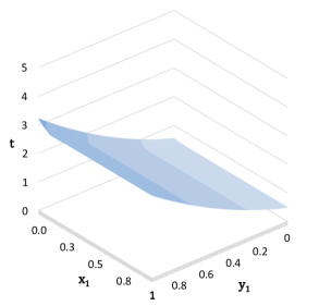
(a) $\text{cl conv}(X_{f})$

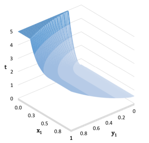
(b) $\text{cl conv}(X_{+})$ (truncated)

Figure 1. Comparison of $\text{cl conv}(X_{f})$ and $\text{cl conv}(X_{+})$. Variables $x_{2}=0.6$, $x_{3}=0.3$, $y_{2}=0.5$, and $y_{3}=0.2$ are fixed.

Outline

The rest of the paper is organized as follows. In §2 we review the valid inequalities for supermodular set functions and present the general form of the lifted supermodular inequalities. In §3 we re-derive known ideal formulations in the literature for quadratic optimization using the lifted supermodular inequalities. In §4 we show that the lifted supermodular inequalities are sufficient to describe the convex hull of $X$. In §5 we provide the explicit form of the lifted supermodular inequalities for $X$, both in the original space of variables and in conic quadratic representable form in an extended space, and discuss the separation problem. In §6 we present computational results, and in §7 we conclude the paper.

Notation

For a set $S\subseteq N$, define $x_{S}$ as the indicator vector of $S$, and define $S_{x}$ as the support set of a vector $x\in\{0,1\}^{N}$. By abusing notation, we use $x_{S}$ and $S_{x}$ interchangeably, e.g., given a set function $g:2^{N}\to\mathbb{R}$, we may equivalently write $g(S)$ or $g(x_{S})$. To simplify the notation, given $i\in N$ and $S\subseteq N$, we write $S\cup i$ instead of $S\cup\{i\}$ and $S\setminus i$ instead of $S\setminus\{i\}$. For a set $Y\subseteq\mathbb{R}^{N}$, let $\text{conv}(Y)$ denote the convex hull of $Y$ and cl conv(Y) denote its closure. We adopt the convention that $a/0=\infty$ if $a>0$ and $a/0=0$ if $a=0$. For a $a\in\mathbb{R}$, let $a_{+}=\max\{a,0\}$. For a vector $c\in\mathbb{R}^{N}$ and a set $S\subseteq N$, we let $c(S)=\sum_{i\in S}c_{i}$ and $\max_{c}(S)=\max_{i\in S}c_{i}$ (by convention, $\max_{c}(\emptyset)=0$).

2. Preliminaries

In this section we cover a few preliminary results for the paper and, at the end, give the general form of the lifted supermodular inequalities (Theorem 1).

2.1. Supermodularity and valid inequalities

A set function $g:2^{N}\to\mathbb{R}$ is supermodular if

$$\rho(i,S)\leq\rho(i,T)\quad\forall i\in N\text{ and }\forall S\subseteq T\subseteq N\setminus i,$$

where $\rho(i,S)=g(S\cup i)-g(S)$ is the increment function.

Proposition 1 (Nemhauser et al [41]).

If $g$ is a supermodular function, then

1. $g(T)\geq g(S)+\sum\limits_{i\in T\setminus S}\rho(i,S)-\sum\limits_{i\in S\setminus T}\rho(i,N\setminus i)$ for all $S,T\subseteq N$

2. $g(T)\geq g(S)+\sum\limits_{i\in T\setminus S}\rho(i,\emptyset)-\sum\limits_{i\in S\setminus T}\rho(i,S\setminus i)$ for all $S,T\subseteq N$.

As a direct consequence of Proposition 1, one can construct valid inequalities for the epigraph of a supermodular function $g$, i.e.,

$$Z=\left\{(x,t)\in\{0,1\}^{N}\times\mathbb{R}:g(x)\leq t\right\}.$$

Specifically, for any $S\subseteq N$, the linear supermodular inequalities [40]

$$g(S)+\sum\limits_{i\in N\setminus S}\rho(i,S)x_{i}-\sum\limits_{i\in S}\rho(i,N\setminus i)(1-x_{i}) \leq t,\text{ and}$$ (3a)

$$g(S)+\sum\limits_{i\in N\setminus S}\rho(i,\emptyset)x_{i}-\sum\limits_{i\in S}\rho(i,S\setminus i)(1-x_{i}) \leq t$$ (3b)

are valid for $Z$.

2.2. Lifted supermodular inequalities

We now describe a family of lifted supermodular inequalities, using a lifting approach similar to the ones used in [28, 46]. Let $h:\{0,1\}^{N}\times\mathbb{R}^{N}\to\mathbb{R}\cup\{\infty\}$ be a function defined over a mixed 0-1 domain and consider its epigraph

$$H=\left\{(x,y,t)\in\{0,1\}^{N}\times\mathbb{R}^{N}\times\mathbb{R}:h(x,y)\leq t\right\}.$$

Observe that $H$ allows for arbitrary constraints, which can be encoded via function $h$. For example, nonnegativity and complementary constraints can be included by letting $h(x,y)=\infty$ whenever $y_{i}<0$ or $y_{i}(1-x_{i})\neq 0$ for some $i\in N$.

For $\alpha\in\mathbb{R}^{N}$, define the set function $g_{\alpha}:\{0,1\}^{N}\to\mathbb{R}\cup\{\infty,-\infty\}$ as

$$g_{\alpha}(x)=\min_{y\in\mathbb{R}^{N}}-\alpha^{\prime}y+h(x,y),$$ (4)

and let $B\subseteq\mathbb{R}^{N}$ be the set of values of $\alpha$ for which problem (4) is bounded, i.e.,

$$B=\left\{\alpha\in\mathbb{R}^{N}:|g_{\alpha}(x)|<\infty,\ \forall x\in\{0,1\}^{N}\right\}.$$

Although supermodularity is defined for set functions only, we propose in Definition 1 below an extension for functions involving continuous variables as well.

Definition 1.

Function $h$ is supermodular if the set function $g_{\alpha}$ defined in (4) is supermodular for all $\alpha\in B$.

Remark 1.

Suppose that $h$ does not depend on the continuous variables $y$, i.e., $h(x,y)=g(x)$. In this case problem (4) is unbounded unless $\alpha=0$, i.e., $B=\{0\}$, and we find that $h(x,y)$ is supermodular if and only if $g_{0}(x)=g(x)$ is supermodular. Thus, Definition 1 includes the usual definition of supermodularity for set functions as a special case. ∎

Proposition 2.

If function $h$ is supermodular, then for any $\alpha\in B$ and $S\subseteq N$, the inequalities

$$\alpha^{\prime}y+g_{\alpha}(S)+\sum\limits_{i\in N\setminus S}\rho_{\alpha}(i,S)x_{i}-\sum\limits_{i\in S}\rho_{\alpha}(i,N\setminus i)(1-x_{i}) \leq t,\text{ and}$$ (5a)

$$\alpha^{\prime}y+g_{\alpha}(S)+\sum\limits_{i\in N\setminus S}\rho_{\alpha}(i,\emptyset)x_{i}-\sum\limits_{i\in S}\rho_{\alpha}(i,S\setminus i)(1-x_{i}) \leq t$$ (5b)

are valid for $H$, where $\rho_{\alpha}(i,S)=g_{\alpha}(S\cup i)-g_{\alpha}(S)$.

Proof.

For any $\alpha\in B$, $S\subseteq N$, and $(x,y,t)\in H$, we find

$$t-\alpha^{\prime}y\geq h(x,y)-\alpha^{\prime}y\geq g_{\alpha}(x)\geq g_{\alpha}(S)+\sum\limits_{i\in N\setminus S}\rho_{\alpha}(i,S)x_{i}-\sum\limits_{i\in S}\rho_{\alpha}(i,N\setminus i)(1-x_{i}),$$

where the first inequality follows directly from the definition of $H$, the second inequality follows by minimizing $h(y)-\alpha^{\prime}y$ with respect to $y$, and the third inequality follows from the validity of (3a). Thus, by adding $\alpha^{\prime}y$ on both sides, we find that inequality (5a) is valid. The validity of (5b) is proven identically. ∎

Since inequalities (5) are valid for any $\alpha\in B$, one can obtain stronger valid inequalities by optimally choosing vector $\alpha$.

Theorem 1 (Lifted supermodular inequalities).

If $h$ is supermodular, then for any $S\subseteq N$, the lifted supermodular inequalities

$$\max_{\alpha\in B}\;g_{\alpha}(S)+\sum\limits_{i\in N\setminus S}\rho_{\alpha}(i,S)x_{i}-\sum\limits_{i\in S}\rho_{\alpha}(i,N\setminus\{i\})(1-x_{i})+\alpha^{\prime}y \leq t,\text{ and}$$ (6a)

$$\max_{\alpha\in B}\;g_{\alpha}(S)+\sum\limits_{i\in N\setminus S}\rho_{\alpha}(i,\emptyset)x_{i}-\sum\limits_{i\in S}\rho_{\alpha}(i,S\setminus\{i\})(1-x_{i})+\alpha^{\prime}y \leq t$$ (6b)

are valid for $H$.

Observe that while inequalities (5) are linear, inequalities (6) are nonlinear in $x$ and $y$. Moreover, each inequality (6) is convex since it is defined as a supremum of linear inequalities. In addition, if the base supermodular inequalities (3) are strong for the convex hull of epi $g_{\alpha}$, then the lifted supermodular inequalities (6) are strong for $H$ as well, as formalized next. Given $\alpha\in B$, define

$$G_{\alpha}=\left\{(x,t)\in\{0,1\}^{N}\times\mathbb{R}:g_{\alpha}(x)\leq t\right\}.$$

Note that $\text{conv}(G_{\alpha})$ is a polyhedron. Theorem 2 below is a direct consequence of Theorem 1 in [46].

Theorem 2 ([46]).

If inequalities (3) and bound constraints $0\leq x\leq 1$ describe $\text{conv}(G_{\alpha})$ for all $\alpha\in B$, then the lifted supermodular inequalities (6) and bound constraints $0\leq x\leq 1$ describe $\text{cl conv}(H)$.

Although Definition 1 may appear to be too restrictive to arise in practice, we show in §2.3 that supermodular functions are in fact widespread in a class of well-studied problems in mixed-integer linear optimization. In §3 we show that several existing results for quadratic optimization with indicators can be obtained as lifted supermodular inequalities. Perhaps, more surprisingly, for the rank-one quadratic with indicators

$$h(x,y)=\begin{cases}\big{(}y(N^{+})-y(N^{-})\big{)}^{2}&\text{if }y\geq 0\text{ and }y_{i}(1-x_{i})=0,\ \forall i\in N^{+}\cup N^{-}\\ \infty&\text{otherwise,}\end{cases}$$

we show in §4 that conditions in Definition 1 and Theorem 2 are satisfied as well.

2.3. Supermodular inequalities and fixed-charge networks

Given $b\in\mathbb{R}$, $u\in\mathbb{R}_{+}^{N}$, and a partition $N=N^{+}\cup N^{-}\cup A^{+}\cup A^{-}$, define for all $x\in\{0,1\}^{N}$ the fixed-charge network set

$$FC(x)=\Big{\{}y\in\mathbb{R}_{+}^{N}:\ y(N^{+})+y(A^{+})-y(A^{-})-y(N^{-})\leq b,\;y_{i}\leq u_{i},\;i\in N,$$

$$y_{i}(1-x_{i})=0,\ i\in N^{+},\;y_{i}x_{i}=0,\ i\in N^{-}\Big{\}}\cdot$$

Wolsey [52] uses $FC(x)$ to describe network structures arising in flow problems with fixed charges on the arcs: $N^{+}$ denotes the incoming arcs into a given subgraph, $N^{-}$ denotes the outgoing arcs, and whereas $A^{+}\cup A^{-}$ denotes the internal arcs in the subgraph, and $b$ represents the supply/demand of the subgraph. Finally, define

$$h(x,y)=\begin{cases}0&\text{if }y\in FC(x)\\ \infty&\text{otherwise.}\end{cases}$$

Proposition 3 ([52]).

For any $\alpha\in\mathbb{R}^{N}$, the function

$$v_{\alpha}(x)=\max_{y\in\mathbb{R}_{+}^{N}}\alpha^{\prime}y-h(x,y)$$

is submodular.

It follows that the function $g_{\alpha}(x)=-v_{\alpha}(x)=\min_{y\in\mathbb{R}_{+}^{N}}-\alpha^{\prime}y+h(x,y)$ is supermodular, and inequalities (5) and (6) are valid. Moreover, Wolsey [52] shows that the linear supermodular inequalities (5) with $\alpha\in\{-1,0,1\}^{N}$ include as special cases well-known inequalities for mixed-integer linear optimization such as flow-cover inequalities [44, 49] and inequalities for capacitated lot-sizing [9, 45]; several other classes for fixed-charge network flow problems are special cases as well [4, 11, 12]. Therefore, the inequalities presented in this paper can be interpreted as nonlinear generalizations of the aforementioned inequalities.

3. Previous results as lifted supermodular inequalities

In order to illustrate the approach, in this section, we show how existing results for quadratic optimization with indicators can be derived using the lifted supermodular inequalities (6).

3.1. The single-variable case

Consider, first, the single-variable case

$$X^{1}=\left\{(x,y,t)\in\{0,1\}\times\mathbb{R}_{+}\times\mathbb{R}:y^{2}\leq t,\;y(1-x)=0\right\}$$

for which $\text{cl conv}(X^{1})$ is given by the perspective reformulation [2, 19, 23, 32]:

$$\text{cl conv}(X^{1})=\left\{(x,y,t)\in[0,1]\times\mathbb{R}_{+}\times\mathbb{R}\cup\infty:\frac{y^{2}}{x}\leq t\right\}.$$

We now derive the perspective reformulation as a special case, in fact, using a modular inequality. Note have that $g_{\alpha}(0)=0$ and $g_{\alpha}(1)=\min_{y\in\mathbb{R}_{+}}-\alpha y+y^{2}=-\frac{\alpha_{+}^{2}}{4}$ since $y^{*}=\alpha/2$ if $\alpha\geq 0$ and $y^{*}=0$ otherwise. Thus, $g_{\alpha}$ is a modular function for any $\alpha\in\mathbb{R}^{N}$, and inequalities (3) reduce to

$$t\geq-\frac{1}{4}\alpha_{+}^{2}x.$$

Then, we find that inequalities (6) reduce to the perspective of $y^{2}$:

$$t\geq\max_{\alpha\in\mathbb{R}^{N}}-\frac{1}{4}\alpha_{+}^{2}x+\alpha y=\frac{y^{2}}{x}\cdot \alpha^{*}=2y/x$$ (with )

3.2. The rank-one case with free continuous variables

Consider the relaxation of $X$ obtained by dropping the non-negativity constraints $y\geq 0$:

$$X_{f}=\big{\{}(x,y,t)\in\{0,1\}^{N}\times\mathbb{R}^{N}\times\mathbb{R}:y(N)^{2}\leq t,\;y_{i}(1-x_{i})=0,\ \forall i\in N\big{\}}\cdot$$

Observe that any rank-one quadratic constraint of the form $\left(\sum_{i\in N}c_{i}y_{i}\right)^{2}\leq t$ with $c_{i}\neq 0$ can be transformed into the form given in $X_{f}$ by scaling the continuous variables (so that $|c_{i}|=1$) and negating variables as $\bar{y}_{i}:=-y_{i}$ if $c_{i}<0$. The closure of the convex hull of $X_{f}$ is derived in [7], and the effectiveness of the resulting inequalities is demonstrated on sparse regression problems. We now re-derive the description of $\text{cl conv}(X_{f})$ using lifted supermodular inequalities.

For $S\subseteq N$, we have

$$g_{\alpha}(x_{S}) =\min_{y\in\mathbb{R}^{S}}-\alpha^{\prime}y+y(S)^{2}.$$

It is easy to see that $g_{\alpha}(x_{S})=-\infty$ unless $\alpha_{i}=\alpha_{j}$ for all $i\neq j$, see [7]. Therefore, letting $\bar{\alpha}=\alpha_{i}$ for all $i\in N$, we find that

$$g_{\bar{\alpha}}(x_{S}) =\min_{y\in\mathbb{R}^{S}}-\bar{\alpha}y(S)+y(S)^{2}=\begin{cases}0&\text{if }S=\emptyset\\ -\bar{\alpha}^{2}/4&\text{otherwise,}\end{cases}$$

where the optimal solution is found by setting $y(S)=\bar{\alpha}/2$. The function $g_{\alpha}$ is supermodular since $\rho_{\bar{\alpha}}(i,\emptyset)=-\bar{\alpha}^{2}/4$ and $\rho_{\bar{\alpha}}(i,S)=0$ for any $S\neq\emptyset$.

Letting $S=\{1\}$, inequality (6a) reduces to

$$\max_{\bar{\alpha}\in\mathbb{R}}\;-\frac{\bar{\alpha}^{2}}{4}+\bar{\alpha}y(N)\leq t\ \Leftrightarrow\ y(N)^{2}\leq t. \bar{\alpha}=2y(N)$$ (with )

Also letting $S=\{1\}$, inequality (6b) reduces to

$$\max_{\bar{\alpha}\in\mathbb{R}}\;-\frac{\bar{\alpha}^{2}}{4}x(N)+\bar{\alpha}y(N)\leq t\ \Leftrightarrow\ \frac{y(N)^{2}}{x(N)}\leq t. \bar{\alpha}=2y(N)/x(N)$$ (with )

These two supermodular inequalities are indeed sufficient to describe $\text{conv}(X_{f})$ [7]. As we shall see in §4, incorporating the non-negativity constraints $y\geq 0$, $\text{conv}(X)$ is substantially more complex than $\text{conv}(X_{f})$. Nonetheless, as shown in Example 1, the resulting convexification is substantially stronger as well.

3.3. The rank-one case with a negative off-diagonal

Consider the special case of $X$ with two continuous variables ($N=\{1,2\}$) with a negative off-diagonal:

$$X_{-}^{2}=\left\{(x,y,t)\in\{0,1\}^{2}\times\mathbb{R}_{+}^{2}\times\mathbb{R}:(y_{1}-y_{2})^{2}\leq t,\;y_{i}(1-x_{i})=0,\ i=1,2\right\}.$$

Observe that any quadratic constraint of the form $\left(c_{1}y_{1}-c_{2}y_{2}\right)^{2}\leq t$ with $c_{1},c_{2}>0$ can be written as in $X_{-}^{2}$ by scaling the continuous variables.

For $\alpha\in\mathbb{R}^{2}$, observe that if $\alpha_{1}+\alpha_{2}>0$,

$$g_{\alpha}(x)=\min_{y\in\mathbb{R}^{2}_{+}}-\alpha_{1}y_{1}-\alpha_{2}y_{2}+(y_{1}-y_{2})^{2}$$

is unbounded. Otherwise,

$$g_{\alpha}(\emptyset) =0,$$

$$g_{\alpha}(\{1\}) =-\frac{\alpha_{1}^{2}}{4}\text{ if }\alpha_{1}\geq 0\text{ and }g_{\alpha}(\{1\})=0\text{ otherwise},$$

$$g_{\alpha}(\{2\}) =-\frac{\alpha_{2}^{2}}{4}\text{ if }\alpha_{2}\geq 0\text{ and }g_{\alpha}(\{2\})=0\text{ otherwise},$$

$$g_{\alpha}(\{1,2\}) =\begin{cases}-\frac{\alpha_{1}^{2}}{4}&\text{if }\alpha_{1}\geq 0\\ -\frac{\alpha_{2}^{2}}{4}&\text{if }\alpha_{2}\geq 0\\ 0&\text{if }\alpha_{1}\leq 0\text{ and }\alpha_{2}\leq 0.\end{cases}$$

In particular, $g_{\alpha}$ is supermodular (and in fact modular) for any fixed $\alpha$ such that $\alpha_{1}+\alpha_{2}\geq 0$: for any $i=1,2$ and $S\subseteq N\setminus i$, $\rho_{\alpha}(i,S)=-\frac{\max\{0,\alpha_{i}\}^{2}}{4}$. Letting $S=\emptyset$, inequality (6a) reduces to

$$\max_{\alpha_{1}+\alpha_{2}\leq 0}\;-\frac{\max\{0,\alpha_{1}\}^{2}}{4}x_{1}-\frac{\max\{0,\alpha_{2}\}^{2}}{4}x_{2}+\alpha_{1}y_{1}+\alpha_{2}y_{2} \leq t.$$ (7)

An optimal solution of (7) can be found as follows. If $y_{1}\geq y_{2}$, then set $\alpha_{1}>0$ and $\alpha_{2}=-\alpha_{1}<0$. Moreover, in this case, the optimal value is given by

$$\max-\frac{\alpha_{1}^{2}}{4}x_{1}+\alpha_{1}(y_{1}-y_{2})=\frac{(y_{1}-y_{2})^{2}}{x_{1}}.$$

The case $y_{2}\geq y_{1}$ is identical. The resulting piecewise valid inequality

$$t\geq\begin{cases}\frac{(y_{1}-y_{2})^{2}}{x_{1}}&\text{if }y_{1}\geq y_{2}\\ \frac{(y_{1}-y_{2})^{2}}{x_{2}}&\text{if }y_{2}\geq y_{1}\end{cases}$$ (8)

along with the bound constraints $0\leq x\leq 1$, $0\leq y$ describe $\text{cl conv}(X_{-}^{2})$ [6]. We point that a conic quadratic representation for $\text{cl conv}(X_{-}^{2})$ and generalizations to (not necessarily rank-one) quadratic functions with negative off-diagonals are given in [13].

3.4. Outlier detection with temporal data

In the context of outlier detection with temporal data, Gómez [29] studies the set

$$X_{T}=\Big{\{}(x,y,t)\in\{0,1\}^{2}\times\mathbb{R}^{4}\times\mathbb{R}: \frac{a_{1}}{2}(y_{3}-y_{1})^{2}+(y_{3}-y_{4})^{2}+\frac{a_{2}}{2}(y_{4}-y_{2})^{2}\leq t,$$

$$y_{1}(1-x_{1})=0,\;y_{2}(1-x_{2})=0\Big{\}}$$

where $a_{1},a_{2}>0$ are constants. While we refer the reader to [29] for details on the derivation of $\text{cl conv}(X_{T})$, we point out that it can in fact be described by lifted supermodular inequalities. Indeed, in this case, function $g_{\alpha}$ is given by

$$g_{\alpha}(x)=K_{1}(\alpha)-K_{2}(\alpha)\max\{x_{1},x_{2}\},$$

where $K_{1}(\alpha)$ and $K_{2}(\alpha)$ are constants that do not depend on $x$ and $K_{2}(\alpha)\geq 0$. Since $\max\{x_{1},x_{2}\}$ is a submodular function, it follows that $g_{\alpha}$ is supermodular.

4. Convex hull via lifted supermodular inequalities

We now turn our attention to the rank-one sets $X$ and $X_{+}$. This section is devoted to showing that the lifted supermodular inequalities (6) are sufficient to describe $\text{cl conv}(X)$ and $\text{cl conv}(X_{+})$. By Theorem 2, it suffices to derive an explicit form of the projection function $g_{\alpha}$ and show that inequalities (3) describe the convex hull of its epigraph $G_{\alpha}$. The rest of this section is organized as follows. In §4.1 we derive the set function $g_{\alpha}$ defined in (4) for the rank-one quadratic function and then show that it is supermodular. In §4.2 we describe the convex hull of $G_{\alpha}$ using only a small subset of the supermodular inequalities (3).

4.1. The set function $g_{\alpha}$

We present the derivation of set function $g_{\alpha}$ for $X_{+}$ and $X$ separately, and then verify that $g_{\alpha}$ is indeed supermodular.

4.1.1. Derivation for $X_{+}$

For $X_{+}$,

$$h(x,y)=\begin{cases}y(N)^{2}&\text{if }y\geq 0\text{ and }y_{i}(1-x_{i})=0,\ \forall i\in N\\ \infty&\text{otherwise.}\end{cases}$$

Therefore, for $S\subseteq N$,

$$g_{\alpha}(x_{S}) =\min_{y\in\mathbb{R}_{+}^{S}}-\alpha^{\prime}y_{S}+y(S)^{2}.$$ (9)

Note that (9) is bounded for all $\alpha\in\mathbb{R}^{S}$, thus $B=\mathbb{R}^{N}$. Since, for $\alpha_{i}<0$, $y_{i}=0$ in any optimal solution, we assume for simplicity that $\alpha\geq 0$ and $B=\mathbb{R}_{+}^{N}$. From the KKT conditions corresponding to variable $y_{k}\geq 0$ in (9), we find that

$$2y(S)\geq\alpha_{k},$$ (10)

and, by complementary slackness, (10) holds at equality whenever $y_{k}>0$. Moreover, let $j\in S$ such that $\alpha_{j}=\max_{\alpha}(S)$; setting $y_{j}=\alpha_{j}/2$ and $y_{i}=0$ for $i\in S\setminus j$, we find a feasible solution for (9) that satisfies all dual feasibility conditions (10) and complementary slackness, and therefore is optimal for the convex optimization problem (9). Thus, we conclude that

$$g_{\alpha}(x_{S})=-\frac{\max_{\alpha}(S)^{2}}{4}\cdot$$

4.1.2. Derivation for $X$

For the general case of $X$,

$$h(x,y)=\begin{cases}\big{(}y(N^{+})-y(N^{-})\big{)}^{2}&\text{if }y\geq 0\text{ and }y_{i}(1-x_{i})=0,\ \forall i\in N^{+}\cup N^{-}\\ \infty&\text{otherwise.}\end{cases}$$

Therefore, for $S\subseteq N^{+}\cup N^{-}$,

$$g_{\alpha}(x_{S}) =\min_{y\in\mathbb{R}_{+}^{S}}-\alpha^{\prime}y+\Big{(}y(N^{+}\cap S)-y(N^{-}\cap S)\Big{)}^{2}.$$ (11)

If $S\cap N^{-}=\emptyset$ or $S\cap N^{+}=\emptyset$, then we find from §4.1.1 that $g_{\alpha}(x_{S})=-\max_{\alpha}(S)^{2}/4$. Now let $S^{+}:=S\cap N^{+}$ and $S^{-}:=S\cap N^{-}$, and assume $S^{+}\neq\emptyset$ and $S^{-}\neq\emptyset$.

Proposition 4.

Problem (11) is bounded if and only if

$$\max_{\alpha}(S^{+})\leq-\max_{\alpha}(S^{-}).$$ (12)

Proof.

Let $p=\operatorname*{arg\,max}_{i\in S^{+}}\alpha_{i}$ and $q=\operatorname*{arg\,max}_{i\in S^{-}}\alpha_{i}$. If $\alpha_{p}+\alpha_{q}>0$ , then $e_{p}+e_{q}$ is an unbounded direction. Otherwise,

$$-\alpha^{\prime}y+\Big{(}y(S^{+})-y(S^{-})\Big{)}^{2} \geq-\alpha_{p}y(S^{+})-\alpha_{q}y(S^{-})+\Big{(}y(S^{+})-y(S^{-})\Big{)}^{2}$$

$$\geq-\alpha_{p}(y(S^{+})-y(S^{-}))+\Big{(}y(S^{+})-y(S^{-})\Big{)}^{2}$$

$$\geq-\alpha_{p}^{2}/4,$$

where the second inequality follows from $\alpha_{p}+\alpha_{q}\leq 0$. ∎

Note that for (12) to hold, if there exists $j\in S^{-}$ such that $\alpha_{j}\geq 0$, then $\alpha_{i}\leq 0$ for all $i\in S^{+}$. Therefore, either $\alpha_{i}\leq 0$ for all $i\in S^{+}$ or $\alpha_{j}\leq 0$ for all $j\in S^{-}$. Also note that we may equivalently rewrite (12) as

$$\alpha_{i}+\alpha_{j}\leq 0,\text{ for all }i\in S^{+},\;j\in S^{-}.$$

First, assume that $\alpha_{j}\leq 0$ for all $j\in S^{-}$. In this case, there exists an optimal solution of (11) where $y(S^{-})=0$ and (11) reduces to (9). Then, we may assume that $\alpha_{i}\geq 0$ for all $i\in S^{+}$ as in §4.1.1, and arrive at

$$g_{\alpha}(x_{S}) =-\frac{\max_{\alpha}(S^{+})^{2}}{4}\cdot$$

By symmetry, if $\alpha_{i}\leq 0$ for all $i\in S^{+}$, we may assume that $\alpha_{j}\geq 0$ for all $i\in S^{-}$ and

$$g_{\alpha}(x_{S}) =-\frac{\max_{\alpha}(S^{-})^{2}}{4}\cdot$$

From the discussion above, we see that we can assume in (6) that

$$B=\left\{\alpha\in\mathbb{R}^{N}:\alpha_{i}\alpha_{j}\leq 0\text{ and }\alpha_{i}+\alpha_{j}\leq 0\ \text{ for all }i\in N^{+},j\in N^{-}\right\}.$$

It is convenient to partition $B$ into two sets so that $B=B^{+}\cup B^{-}$, where

$$B^{+} =\left\{\alpha\in\mathbb{R}^{N}:\alpha_{i}\geq 0\ \forall i\in N^{+},\alpha_{j}\leq 0\ \forall j\in N^{-},\text{ and }\alpha_{i}+\alpha_{j}\leq 0\ \forall i\in N^{+},j\in N^{-}\right\}$$

$$B^{-} =\left\{\alpha\in\mathbb{R}^{N}:\alpha_{i}\leq 0\ \forall i\in N^{+},\alpha_{j}\geq 0\ \forall j\in N^{-},\text{ and }\alpha_{i}+\alpha_{j}\leq 0\ \forall i\in N^{+},j\in N^{-}\right\}$$

and analyze the inequalities separately for each set. Figure 2 depicts regions $B^{+}$ and $B^{-}$ for a two-dimensional case.

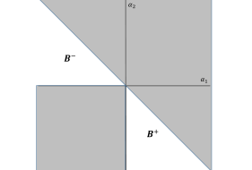
Figure 2. Depiction of $B^{+}$ and $B^{-}$ in a two-dimensional example with $N^{+}=\{1\}$ and $N^{-}=\{2\}$. The upper right shaded region (triangle) corresponds to the region where $g_{\alpha}(x)=-\infty$; the lower left shaded region (square) corresponds to the region discarded, as optimal solutions of (6) can be found in either $B^{+}$ or $B^{-}$.

Therefore, instead of studying inequalities (6) directly, one can equivalently study their relaxation where either $\alpha\in B^{+}$ or $\alpha\in B^{-}$; consequently, each inequality (6) corresponds to (the maximum of) two simpler inequalities. Since the sets $B^{+}$ and $B^{-}$ are symmetric, and inequalities (6) corresponding to $\alpha\in B^{-}$ are simply inequalities where the role of $N^{+}$ and $N^{-}$ is interchanged (and $\alpha\in B^{+}$), the analysis and derivation of the inequalities is simplified. Therefore, in the sequel, we will derive the inequalities for $\alpha\in B^{+}$ only and then state the inequalities corresponding to $B^{-}$ by interchanging $N^{+}$ and $N^{-}$.

Supermodularity

For $\alpha\in B^{+}$, the set function $g_{\alpha}(x)$ for $X$ is monotone non-increasing, also it is supermodular as $\max_{\alpha}(S^{+})$ is submodular. The case for $\alpha\in B^{-}$ is analogous.

4.2. Convex hull of epi $g_{\alpha}$

In this section we show that a small subset of the supermodular inequalities (3a) are sufficient to describe the convex hull of the epigraph of the set function $g_{\alpha}$, i.e.,

$$G_{\alpha}=\left\{(x,t)\in\{0,1\}^{N}\times\mathbb{R}:-\frac{\max_{i\in N}\{\alpha_{i}^{2}x_{i}\}}{4}\leq t\right\}\cdot$$ (13)

Given nonempty $S\subseteq N$, $\ell\in\operatorname*{arg\,max}_{i\in S}\{\alpha_{i}\}$, $k\in\operatorname*{arg\,max}_{i\in N\setminus\ell}\{\alpha_{i}\}$, and $T=\left\{i\in N\setminus S:\alpha_{i}>\alpha_{\ell}\right\}$; observe that $T=\emptyset$ if and only if $\alpha_{\ell}\geq\alpha_{k}$. Then, valid inequalities (3a) for $G_{\alpha}$ reduce to

$$t\geq\begin{cases}-\frac{\alpha_{\ell}^{2}}{4}+\frac{\alpha_{\ell}^{2}-\alpha_{k}^{2}}{4}(1-x_{\ell})&\text{if }\alpha_{\ell}\geq\alpha_{k}\\ -\frac{\alpha_{\ell}^{2}}{4}-\sum\limits_{i\in T}\frac{\alpha_{i}^{2}-\alpha_{\ell}^{2}}{4}x_{i}&\text{if }\alpha_{\ell}\leq\alpha_{k}.\end{cases}$$ (14)

If $S=\emptyset$, then valid inequalities (3a) reduce to

$$t\geq-\sum\limits_{i\in N}\frac{\alpha_{i}^{2}}{4}x_{i}.$$

Remark 2.

Observe that if $\alpha_{\ell}\geq\alpha_{k}$, then the inequality

$$t\geq-\frac{\alpha_{\ell}^{2}}{4}+\frac{\alpha_{\ell}^{2}-\alpha_{k}^{2}}{4}(1-x_{\ell})=-\frac{\alpha_{k}^{2}}{4}-\frac{\alpha_{\ell}^{2}-\alpha_{k}^{2}}{4}x_{\ell}$$

can also be obtained by setting $S=N\setminus\ell$ (or by choosing any $S\subseteq N\setminus\ell$ such that $k\in S$). Therefore, when considering inequalities (14), we can assume without loss of generality that there exists $k\in\operatorname*{arg\,max}_{i\in N}\{\alpha_{i}\}$ such that $k\not\in S$ and, thus, the case $\alpha_{\ell}\geq\alpha_{k}$ can be ignored. ∎

Remark 3.

Suppose that the variables are indexed such that $\alpha_{1}\leq\ldots\leq\alpha_{n}$, let $\alpha_{0}=0$, and let $\ell=\max_{i\in S}\{i\}$ if $S\neq\emptyset$ and $\ell=0$ otherwise. Observe that we can assume without loss of generality that $i\in S$ for all $i\leq\ell$, since inequalities (14) are the same whether $i\in S$ or not. Therefore, it follows that there are only $n$ inequalities (14) given by

$$t\geq-\frac{\alpha_{\ell}^{2}}{4}-\sum_{i=\ell+1}^{n}\frac{\alpha_{i}^{2}-\alpha_{\ell}^{2}}{4}x_{i},\quad\ell=0,\ldots,n-1.$$ (15)

We now show that inequalities (14) characterize the convex hull of $G_{\alpha}$.

Proposition 5.

Inequalities (14) and bound constraints describe $\text{conv}(G_{\alpha})$.

Proof.

Let $(x,t)\in[0,1]^{N}\times\mathbb{R}$. By definition, $(x,t)\in\text{conv}(G_{\alpha})$ if and only

$$t\geq\min_{\lambda}\; -\sum_{S\subseteq N}\frac{\max_{\alpha}(S)^{2}}{4}\lambda_{S}$$ (16a)

s.t. $$\sum_{S\subseteq N:i\in S}\lambda_{S}=x_{i},\ \ i\in N$$ (16b)

$$\sum_{S\subseteq N}\lambda_{S}=1$$ (16c)

$$\lambda_{S}\geq 0,\ \ S\subseteq N,$$ (16d)

where constraints (16b) can be restated as $x=\sum_{i\in S}\lambda_{S}x_{S}$. From linear programming duality, we find the equivalent condition

$$t\geq\max_{\mu,\gamma}\; \sum_{i\in N}x_{i}\mu_{i}+\gamma$$ (17a)

s.t. $$\sum_{i\in S}\mu_{i}+\gamma\leq-\frac{\max_{\alpha}(S)^{2}}{4},\ \ S\subseteq N$$ (17b)

$$\mu\in\mathbb{R}^{N},\;\gamma\in\mathbb{R}.$$ (17c)

Any feasible solution $(\mu,\gamma)$ of (17) yields a valid inequality for $\text{conv}(G_{\alpha})$. Moreover, characterizing the optimal solutions of (17) (for all $x\in[0,1]^{N}$) results in the convex hull description of $G_{\alpha}$.

Suppose, without loss of generality, that $\alpha_{1}\leq\ldots\leq\alpha_{n}$, let $\alpha_{0}=0$, and let $\ell\in\{0,\ldots,n-1\}$ be the smallest index such that $\sum_{i=\ell+1}^{n}x_{i}\leq 1$; thus, if $\ell>0$, then $\sum_{i=\ell}^{n}x_{i}>1$. We claim that the dual solution given by $\hat{\gamma}=-\frac{\alpha_{\ell}^{2}}{4}$, $\hat{\mu}_{i}=0$ for $i\leq\ell$ and $\hat{\mu}_{i}=-\frac{\alpha_{i}^{2}-\alpha_{\ell}^{2}}{4}$ for $i>\ell$ is optimal for (17).

First, we verify that $(\hat{\mu},\hat{\gamma})$ is feasible for (17). Observe that for any $S\subseteq\{1,\ldots,\ell\}$, constraint (17b) reduces to $-\frac{\alpha_{\ell}^{2}}{4}\leq-\frac{\max_{\alpha}(S)^{2}}{4}$, which is indeed satisfied. For any $S$ such that the maximum element $j>\ell$, we find that (17b) reduces to $\sum_{i\in S:i\neq j}\hat{\mu}_{i}\leq 0$; since $\hat{\mu}\leq 0$, the constraint is satisfied. For $S=\emptyset$, constraint (17b) reduces to $\gamma\leq 0$, which is satisfied. To verify complementary slackness (later), note that constraints (17b) corresponding to sets (a) $S=T\cup\{j\}$, where $T\subseteq\{1,\ldots,\ell\}$ and $j>\ell$ (i.e., containing exactly one element greater than $\ell$), and (b) $S=T\cup\{\ell\}$, where $T\subseteq\{1,\ldots,\ell-1\}$ (i.e., containing $\ell$ but no greater element) are satisfied at equality.

Finally, for $(\hat{\mu},\hat{\gamma})$, the objective function (17a) is of the form (15):

$$t\geq-\frac{\alpha_{\ell}^{2}}{4}-\sum_{i=\ell+1}^{n}\frac{\alpha_{i}^{2}-\alpha_{\ell}^{2}}{4}x_{i}.$$

To verify that $(\hat{\mu},\hat{\gamma})$ is optimal for (17), we construct a primal solution $\hat{\lambda}$ feasible for (16) satisfying complementary slackness. The greedy algorithm for constructing $\hat{\lambda}$ is presented in Algorithm 1 and illustrated with an example in Figure 3.

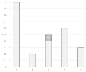
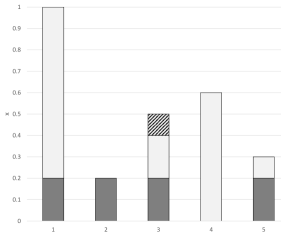
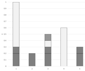
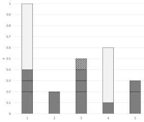
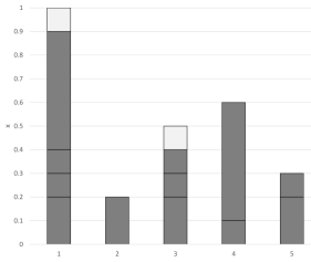
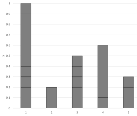
(a) Buffer $1-x_{4}-x_{5}=0.1$ for index $\ell=3$, $\hat{\lambda}=0$ (b) $\hat{\lambda}_{1,2,3,5}\leftarrow x_{2}=0.2$. Constraint (16b) for $x_{2}$ is met (c) $\hat{\lambda}_{1,3,5}\leftarrow x_{5}-x_{2}=0.1$. Constraint (16b) for $x_{5}$ is met (d) $\hat{\lambda}_{1,3,4}\leftarrow 0.1$. Constraint (16b) for $x_{3}$ is not met due to the buffer (e) $\hat{\lambda}_{1,4}\leftarrow 0.5$. Constraint (16b) for $x_{4}$ is met and the buffer is removed (f) $\hat{\lambda}_{1,3}\leftarrow 0.1$. Constraints (16b) for $x_{1},x_{3}$ and (16c) are met Figure 3. Algorithm 1 with $x=(1,0.2,0.5,0.6,0.3)$ and $\ell=3$.

Algorithm 1 Algorithm for problem (16)

1:$x_{1},\dots,x_{n}$ with $0=:\alpha_{0}\leq\alpha_{1}\leq\dots\leq\alpha_{n}$.

2:$\hat{\lambda}$ optimal for (16).

3:$\ell\leftarrow\min\{k:\sum_{i=k+1}^{n}x_{i}\leq 1\}$

4:$\hat{\lambda}_{S}\leftarrow 0$ for all $S\subseteq N$

5:$\hat{x}_{i}\leftarrow x_{i}$ for all $i\in N\setminus\ell$

6:if $\ell>0$ then

7:    $\hat{x}_{\ell}\leftarrow x_{\ell}-\left(1-\sum_{i=\ell+1}^{n}x_{i}\right)$ $\triangleright$ Buffer for $\ell$; $\hat{x}_{\ell}>0$ by definition of $\ell$

8:end if

9:$\Lambda\leftarrow 0$ $\triangleright$ Variable for $\sum_{S}\hat{\lambda}_{S}$

10:for $j=n\ldots\ell+1$ do

11:    while $\hat{x}_{j}>0$ do

12:         $S\leftarrow\{i\leq\ell:\hat{x}_{i}>0\}\cup j$

13:         Allocate($S$)

14:    end while

15:end for $\triangleright$ At this point $\Lambda=\sum_{i={\ell+1}}^{n}x_{i}$

16:if $\ell=0$ then

17:    $\hat{\lambda}_{\emptyset}\leftarrow 1-\Lambda$ $\triangleright$ Constraint (16c) is satisfied

18:    $\Lambda\leftarrow 1$

19:else

20:    $\hat{x}_{\ell}\leftarrow 1-\sum_{i=\ell+1}^{n}x_{i}$$\triangleright$ Buffer is removed

21:    while $\hat{x}_{\ell}>0$ do

22:         $S\leftarrow\{i<\ell:\hat{x}_{i}>0\}\cup\ell$

23:         Allocate($S$)

24:    end while $\triangleright$ $\Lambda=1$

25:end if

26:return $\hat{\lambda}$

27:

28:function Allocate($S$)

29:    $v\leftarrow\min_{i\in S}\hat{x}_{i}$

30:    $\Lambda\leftarrow\Lambda+v$

31:    $\hat{\lambda}_{S}\leftarrow v$

32:    $\hat{x}_{i}\leftarrow\hat{x}_{i}-v$ for all $i\in S$ $\triangleright$ At this point $\hat{x}_{i}=\left(x_{i}-\Lambda\right)_{+}$ for all $i<\ell$

33:end function

We now check that constraint (16c) is satisfied. At the end of the algorithm, $\sum_{S\subseteq N}\hat{\lambda}_{S}=\Lambda$ (since variable $\Lambda$ is updated each time $\hat{\lambda}$ is updated). Moreover, at the end of the first cycle (line 15) we have $\Lambda=\sum_{i=\ell+1}^{n}x_{i}$. If $\ell=0$, then $\Lambda=1$ trivially (line 18); otherwise, at the end of the second cycle (line 24) and additional value of $\hat{x}_{\ell}=1-\sum_{i=\ell+1}^{n}x_{i}$ (line 20) is added to $\Lambda$. Hence, at the end of the algorithm

$$\Lambda=\sum_{S\subseteq N}\hat{\lambda}_{S}=\sum_{i=\ell+1}^{n}x_{i}+\left(1-\sum_{i=\ell+1}^{n}x_{i}\right)=1.$$

Next, we verify that constraints (16b) are satisfied. For $i\in\{1,\ldots,\ell-1\}$, at any point in the algorithm, we have that $\sum_{S\subseteq N:i\in S}\lambda_{S}=x_{i}-\hat{x}_{i}$. Since, at any point, $\hat{x}_{i}=\left(x_{i}-\Lambda\right)_{+}$ and $\Lambda=1$ at the end of the algorithm, it follows that $\sum_{S\subseteq N:i\in S}\lambda_{S}=x_{i}$. For $i\in\{\ell+1,\ldots,n\}$ we also have that $\sum_{S\subseteq N:i\in S}\lambda_{S}=x_{i}-\hat{x}_{i}$, and $\hat{x}_{i}=0$ at the end (line 15). Finally, for $i=\ell>0$, we have that

$$\sum_{S\subseteq N:\ell\in S}\lambda_{S}=\left(x_{\ell}-\left(1-\sum_{i=\ell+1}^{n}x_{i}\right)\right)+\left(1-\sum_{i=\ell+1}^{n}x_{i}\right)=x_{\ell}.$$

Finally, to check that $\hat{\lambda}$ satisfies complementary slackness, it suffices to observe that all updates of $\hat{\lambda}$ correspond to sets $S$ such that exactly one element of $S$ is greater than $\ell$ (line 12), or to sets $S$ with no element greater than $\ell$ and where $\ell\in S$ (line 22), where the corresponding dual constraints are satisfied at equality.

Therefore, we conclude that $\hat{\lambda}$ and $(\hat{\mu},\hat{\gamma})$ are an optimal primal-dual pair. Since problem (17) admits for any $x\in[0,1]$ an optimal solution of the form (15), it follows that those inequalities and bound constraints describe $\text{conv}(G_{\alpha})$. ∎

Finally, we obtain the main result of this section: that the (nonlinear) lifted supermodular inequalities

$$t\geq \max_{\alpha\in B^{+}}-\frac{\max_{\alpha}(S^{+})^{2}}{4}-\sum\limits_{i\in N^{+}\setminus S^{+}}\frac{\left(\alpha_{i}^{2}-\max_{\alpha}(S^{+})^{2}\right)_{+}}{4}x_{i}+\alpha^{\prime}y,\ \ \forall S^{+}\subseteq N^{+}$$ (18)

$$t\geq \max_{\alpha\in B^{-}}-\frac{\max_{\alpha}(S^{-})^{2}}{4}-\sum\limits_{i\in N^{-}\setminus S^{-}}\frac{\left(\alpha_{i}^{2}-\max_{\alpha}(S^{-})^{2}\right)_{+}}{4}x_{i}+\alpha^{\prime}y,\ \ \forall S^{-}\subseteq N^{-}$$ (19)

are sufficient to describe the closure of the convex hull of $X$.

Proposition 6.

Lifted supermodular inequalities (18)–(19) and the bound constraints $0\leq x\leq 1$, $y\geq 0$ describe $\text{cl conv}(X)$.

Proof.

Follows immediately from Proposition 5 and Theorem 2. ∎

Remark 4.

We end this section with the remark that optimization of a linear function over $X$ can be done easily using the projection function $g_{\alpha}$. Consider

$$\min\big{\{}-\alpha^{\prime}y+\beta^{\prime}x+t:(x,y,t)\in X\big{\}}\cdot$$

Projecting out the continuous variables using $g_{\alpha}$, the problem reduces to

$$\min_{x\in\{0,1\}^{N}}\beta^{\prime}x-\max_{i\in N}\{\alpha_{i}^{2}x_{i}\}/4,$$

which can be solved in linear time.

5. Explicit form of the lifted supermodular inequalities

In this section we derive explicit forms of the lifted supermodular inequalities (18)–(19). In §5.1 we describe the inequalities in the original space of variables, and describe how to solve the separation problem. In §5.2 we provide conic quadratic representable inequalities in an extended space, which can then be implemented with off-the-shelf conic solvers.

5.1. Inequalities and separation in the original space of variables

5.1.1. Lifted inequalities for $X$

We first present the inequalities for the more general set $X$. Finding a closed form expression for the lifted supermodular inequalities (18) for all $S^{+}\subseteq N^{+}$ amounts to solving the maximum lifting problem

$$t\geq\max_{S^{+}\subseteq N^{+},\alpha\in B^{+}}-\frac{\max_{\alpha}(S^{+})^{2}}{4}-\sum\limits_{i\in N^{+}\setminus S^{+}}\frac{\left(\alpha_{i}^{2}-\max_{\alpha}(S^{+})^{2}\right)_{+}}{4}x_{i}+\alpha^{\prime}y.$$ (20)

Proposition 7.

Given $(x,y)\in[0,1]^{N}\times\mathbb{R}_{+}^{N}$, if there exist disjoint sets $L,U\subseteq N^{+}$ such that

$$1-x(N^{+}\setminus L)\geq 0$$ (21a)

$$\frac{y(L)}{1-x(N^{+}\setminus L)}<\frac{y_{i}}{x_{i}},\quad i\in N^{+}\setminus L$$ (21b)

$$\frac{y(L)}{1-x(N^{+}\setminus L)}\geq\frac{y_{i}}{x_{i}},\quad i\in L$$ (21c)

$$y(U)-y(N^{-})\geq 0$$ (21d)

$$\frac{y(U)-y(N^{-})}{x(U)}>\frac{y_{i}}{x_{i}},\quad i\in N^{+}\setminus U$$ (21e)

$$\frac{y(U)-y(N^{-})}{x(U)}\leq\frac{y_{i}}{x_{i}},\quad i\in U$$ (21f)

$$\frac{y(L)}{1-x(N^{+}\setminus L)}<\frac{y(U)-y(N^{-})}{x(U)},$$ (21g)

then inequality (20) reduces to

$$t\geq\frac{y(L)^{2}}{1-x(N^{+}\setminus L)}+\sum\limits_{i\in N^{+}\setminus(L\cup U)}\frac{y_{i}^{2}}{x_{i}}+\frac{\big{(}y(U)-y(N^{-})\big{)}^{2}}{x(U)};$$ (22)

otherwise, inequality (20) reduces to $t\geq\big{(}y(N^{+})-y(N^{-})\big{)}^{2}$.

Below we state two remarks on Proposition 7, and then we prove the result.

Remark 5.

Inequalities (22) are neither valid for $\text{cl conv}(X)$ nor convex for all $(x,y)\in[0,1]^{N}\times\mathbb{R}_{+}^{N}$. Indeed, if condition (21a) is not satisfied, then (22) may not be convex. Moreover, suppose that $L=\{j\}$ and $U=\{k\}$ for some $j,k\in S^{+}$: note that setting $x_{i}=y_{i}=0$ for all $i\in N\setminus\{j,k\}$, $x_{j}=x_{k}=1$, $y_{j},y_{k}>0$, and $t=(y_{j}+y_{k})^{2}$ is feasible for $X$, but this point is cut off by inequality (22) since $\frac{y(L)^{2}}{1-x(N^{+}\setminus L)}=\frac{y_{j}^{2}}{1-x_{k}}=\infty$.

In fact, if $(x,y,t)\in\text{cl conv}(X)$, then (22) is guaranteed to hold only when conditions (21a), (21b), (21d), (21e), and (21g) are satisfied. Conditions (21c) and (21f) do not affect the validity of (22) but if they are not satisfied then (22) is weak, i.e., a stronger inequality can be obtained from another choice of $L$ and $U$. ∎

Remark 6.

If $y(N^{+})<y(N^{-})$, there exists no $L$ and $U$ satisfying condition (21d) in Proposition 7. However, in this case, the role of $N^{+}$ and $N^{-}$ can be interchanged to satisfy (21d); interchanging $N^{+}$ and $N^{-}$ is equivalent to letting $\alpha\in B^{-}$. ∎

Proof of Proposition 7.

Let us define variables auxiliary variables $\beta,\gamma\in\mathbb{R}$ as $\beta=\max_{\alpha}(N^{-})$ and $\gamma=\max_{\alpha}(S^{+})$, respectively. Then, inequality (20) reduces to

$$t\geq\max_{S^{+}\subseteq N^{+}}\max_{\alpha,\beta,\gamma} -\frac{\gamma^{2}}{4}-\sum\limits_{i\in N^{+}\setminus S^{+}}\frac{\left(\alpha_{i}^{2}-\gamma^{2}\right)_{+}}{4}x_{i}+\alpha^{\prime}y$$ (23a)

s.t. $$\alpha_{i}\leq\gamma,\ \ \ \ \ \ \forall i\in S^{+}$$ (23b)

$$\alpha_{i}\leq\beta,\ \ \ \ \ \forall i\in N^{-}$$ (23c)

$$\beta\leq-\alpha_{i},\ \ \forall i\in N^{+}$$ (23d)

$$\alpha\in\mathbb{R}^{N},\;\gamma\in\mathbb{R}_{+},\beta\in\mathbb{R}_{-},$$ (23e)

where constraints (23b) and (23c) enforce the definitions of $\gamma$ and $\beta$, and constraints (23d) and (23e) enforce that $\alpha\in B^{+}$.

First, observe that there exists an optimal solution of (23) with $\gamma\leq\alpha_{i}$ for all $i\in N^{+}$: if $\alpha_{i}<\gamma$ for some $i\in N^{+}$, then setting $\alpha_{i}=\gamma$ results in a feasible solution with improved objective value. Therefore, the value of $S^{+}$ is completely determined by $\gamma$ since $S^{+}=\left\{i\in N^{+}:\alpha_{i}\leq\gamma\right\}$ Also note that $\alpha_{i}=\beta$ for all $i\in N^{-}$: if $\alpha_{i}<\beta$ for some $i\in N^{-}$, then setting $\alpha_{i}=\beta$ results in an improved objective value. We now consider two cases:

Case 1

Suppose in an optimal solution of (23) we have $\gamma=-\beta$, which implies that $\alpha_{i}=\gamma$ for all $i\in N^{+}$ and $\alpha_{i}=-\gamma$ for all $i\in N^{-}$. In this case, (23) simplifies to $t\geq\max_{\gamma\in\mathbb{R}_{+}}\gamma\big{(}y(N^{+})-y(N^{-})\big{)}-\frac{\gamma^{2}}{4},$ which, after optimizing for $\gamma$, further reduces to the original rank-one quadratic inequality $t\geq\big{(}y(N^{+})-y(N^{-})\big{)}^{2}.$

Case 2

Now suppose $\gamma<-\beta$ in an optimal solution. Let $L=\left\{i\in N^{+}:\alpha_{i}=\gamma\right\}$ and $U=\{i\in N^{+}:\alpha_{i}=-\beta\}$. Then, from the discussion above, (23) reduces to

$$t\geq\max_{\alpha,\beta,\gamma}\; \gamma\cdot y(L)-\frac{\gamma^{2}}{4}\big{(}1-x(N^{+}\setminus L)\big{)}+\sum\limits_{i\in N^{+}\setminus(L\cup U)}\left(\alpha_{i}y_{i}-\frac{\alpha_{i}^{2}}{4}x_{i}\right)$$

$$-\beta\big{(}y(U)-y(N^{-})\big{)}-\frac{\beta^{2}}{4}x(U)$$ (24a)

s.t. $$\gamma<\alpha_{i}<-\beta,\ \ \ \forall i\in N^{+}\setminus(L\cup U)$$ (24b)

$$\alpha\in\mathbb{R}^{N},\;\gamma,\beta\in\mathbb{R}_{+}.$$ (24c)

Observe that for $(L,U,\gamma)$ to correspond to an optimal solution, we must have $1-x(N^{+}\setminus L)\geq 0$ (otherwise, $\gamma$ can be increased to another $\alpha_{i}$ while improving the objective value) and $y(U)-y(N^{-})\geq 0$ (otherwise, $-\beta$ can be decreased to another $\alpha_{i}$ while improving the objective value). When both conditions are satisfied, from first-order conditions we see that $\alpha_{i}=2y_{i}/x_{i}$ for $i\in N^{+}\setminus(L\cup U)$, $\gamma=2y(L)/\big{(}1-x(N^{+}\setminus L)\big{)}$ and $\beta=-2\big{(}y(U)-y(N^{-})\big{)}/x(U)$, and (24) simplifies to (22). The constraints $\gamma<\alpha_{i}$ are satisfied for all $i\in N^{+}\setminus(L\cup U)$ if and only if (21b) hold, constraints $\alpha_{i}\leq-\beta$ are satisfied for all $i\in N^{+}\setminus(L\cup U)$ if and only if (21e) hold, and constraint $\alpha<-\beta$, which may not be implied if $N^{+}\setminus(L\cup U)=\emptyset$, is satisfied if and only if (21g) holds.

Finally, we verify that first order conditions are satisfied for $j\in L$, this is, setting $\alpha_{j}>\gamma$ results in a worse solution. If condition (21c)

$$\frac{y(L)}{1-x(N^{+}\setminus L)}\geq\frac{y_{i}}{x_{i}},\quad\forall i\in L$$

does not hold for some $j\in L$, then increasing $\alpha_{j}$ from $\gamma=2\frac{y(L)}{1-x(N^{+}\setminus L)}$ to $2y_{j}/x_{j}$ improves the objective value. Similarly, we verify that first order conditions for $j\in U$: if condition (21f)

$$\frac{y(U)-y(N^{-})}{x(U)}\leq\frac{y_{i}}{x_{i}},\quad\forall i\in U$$

does not hold for some $j\in U$, then $\alpha_{j}$ can be decreased from $\beta=\frac{y(U)-y(N^{-})}{x(U)}$ to improve the objective value. ∎

5.1.2. Lifted inequalities for $X_{+}$

We now present the inequalities for $X_{+}$, which can be interpreted as a special cases of the inequalities for $X$ given in §5.1.1. Recall that for set $X_{+}$, the set $B$ used in (6a) is simply $B=\mathbb{R}^{N}$ (we can assume $B=\mathbb{R}_{+}^{N}$ without loss of generality) and a closed form expression for (6a) requires solving the lifting problem

$$t\geq\max_{S\subseteq N}\max_{\alpha\in\mathbb{R}_{+}^{N}}-\frac{\max_{\alpha}(S)^{2}}{4}-\sum\limits_{i\in N\setminus S}\frac{\left(\alpha_{i}^{2}-\max_{\alpha}(S)^{2}\right)_{+}}{4}x_{i}+\alpha^{\prime}y.$$ (25)

Note that in the proof of Proposition 7, set $U$ corresponds to the set of variables in $N^{+}$ where constraint $\alpha_{i}\leq-\max_{\alpha}(N^{-})$ is tight in an optimal solution of (23). Intuitively, set $X_{+}$ can be interpreted as a special case of $X$ where $N^{+}=N$ and $N^{-}=\emptyset$, and such constraints can be dropped from the lifting problem. Therefore, we may assume $U=\emptyset$ in Proposition 7. Proposition 8 formalizes this intuition; note however that it is slightly stronger as, unlike Proposition 7, it guarantees the existence of a set satisfying the conditions of the proposition.

Proposition 8.

Given any $(x,y)\in[0,1]^{N}\times\mathbb{R}_{+}^{N}$, there exists a (possibly empty) set $L\subseteq N$ such that

$$1-x(N\setminus L)\geq 0$$ (26a)

$$\frac{y(L)}{1-x(N\setminus L)}<\frac{y_{i}}{x_{i}},\quad i\in N\setminus L$$ (26b)

$$\frac{y(L)}{1-x(N\setminus L)}\geq\frac{y_{i}}{x_{i}},\quad i\in L$$ (26c)

and inequality (25) reduces to

$$t\geq\frac{y(L)^{2}}{1-x(N\setminus L)}+\sum\limits_{i\in N\setminus L}\frac{y_{i}^{2}}{x_{i}}.$$ (27)

The proof of Proposition 8 is given in Appendix A.

Example 1 (cont).

Consider $X_{+}$ with $n=3$, and assume $x_{2}=0.6$, $x_{3}=0.3$, $y_{2}=0.5$ and $y_{3}=0.2$. Note that $y_{2}/x_{2}\approx 0.83>0.67\approx y_{3}/x_{3}$. We now compute the minimum values $t$ such $(x,y,t)\in\text{cl conv}(X_{+})$, for different values of $(x_{1},y_{1})$.

$\bullet$ Let $(x_{1},y_{1})=(0.01,1)$ and $y_{1}/x_{1}=100$. Then $L=\emptyset$ satisfies all conditions (21): $x(N)=0.91<1$, conditions (26b) are trivially satisfied since $y(\emptyset)=0$, and conditions (26c) are void. In this case, we find that $(x,y,t)\in\text{cl conv}(X_{+})$ iff $t\geq 1^{2}/0.01+0.5^{2}/0.6+0.2^{2}/0.3\approx 100.55$. In contrast, $(x,y,t)\in\text{cl conv}(X_{f})$ iff $t\geq\left(0.01+0.5+0.2\right)^{2}/0.91\approx 3.18$.

$\bullet$ Let $(x_{1},y_{1})=(0.1,0.5)$ and $y_{1}/x_{1}=5$. Then $L=\{3\}$ satisfies all conditions (21): $x_{1}+x_{2}=0.7<1$, $0.2/0.3\approx 0.67<y_{2}/x_{2}$ and $0.2/0.3\approx 0.67=y_{3}/x_{3}$. In this case, $(x,y,t)\in\text{cl conv}(X_{+})$ iff $t\geq 0.2^{2}/0.3+0.5^{2}/0.1+0.5^{2}/0.6\approx 3.05$. In contrast, $(x,y,t)\in\text{cl conv}(X_{f})$ iff $t\geq\left(0.5+0.5+0.2\right)^{2}/1=1.44$.

$\bullet$ Let $(x_{1},y_{1})=(0.4,0.1)$ and $y_{1}/x_{1}=0.25$. Then $L=\{1,3\}$ satisfies all conditions (21): $x_{2}=0.6<1$, $(0.1+0.2)/0.4=0.75<y_{2}/x_{2}$ and $(0.1+0.2)/0.4=0.75\geq y_{3}/x_{3}$. In this case, $(x,y,t)\in\text{cl conv}(X_{+})$ iff $t\geq(0.1+0.2)^{2}/0.4+0.5^{2}/0.6\approx 0.642$. In contrast, $(x,y,t)\in\text{cl conv}(X_{f})$ iff $t\geq\left(0.1+0.5+0.2\right)^{2}=0.640$.

$\bullet$ Let $(x_{1},y_{1})=(0.5,0.2)$ and $y_{1}/x_{1}=0.4$. Then $L=\{1,2,3\}$ satisfies all conditions (21): (26a) is trivially satisfied, (26b) is void and $(0.2+0.5+0.2)/1=0.9\geq y_{2}/x_{2}$. In this case, $(x,y,t)\in\text{cl conv}(X_{+})$ iff $t\geq(0.2+0.5+0.2)^{2}=0.81$, which coincides with $\text{cl conv}(X_{f})$ and the natural inequality $t\geq y(N)^{2}$.

Figure 1 plots the minimum values of $t$ as a function of $(x_{1},y_{1})$ for $\text{cl conv}(X_{f})$ and $\text{cl conv}(X_{+})$. ∎

5.1.3. Separation

We now consider the separation problem for inequalities (20) and (25), i.e., given a point $(\bar{x},\bar{y})\in[0,1]^{N}\times\mathbb{R}_{+}^{N}$, finding sets $L,U\subseteq N^{+}$ satisfying the conditions in Proposition 7 or finding $L\subseteq N$ satisfying the conditions in Proposition 8, respectively.

Separation for (20)

First, as pointed out in Remark 6, we verify whether $\bar{y}(N^{+})\geq\bar{y}(N^{-})$ or $\bar{y}(N^{+})<\bar{y}(N^{-})$; in the first case, we use directly the conditions in Proposition 7, and in the second one, we interchange the roles of $N^{+}$ and $N^{-}$ so that $\bar{y}(N^{+})\geq\bar{y}(N^{-})$. Next, index the variables so that $\bar{y}_{1}/\bar{x}_{1}\leq\bar{y}_{2}/\bar{x}_{2}\leq\ldots\leq\bar{y}_{m}/\bar{x}_{m}$, where $m=|N^{+}|$, which is done in $O(m\log m)$ by sorting. It follows from the conditions in Proposition 7 that if such sets $L,U\subseteq N^{+}$ exist, then $L=\left\{i\in N^{+}:i\leq\ell\right\}$ and $U=\left\{i\in N^{+}:i\geq u\right\}$ for some $\ell,u\in\{1,\ldots,m\}$ with $\ell<u$. Therefore, one can simply enumerate all $m(m-1)/2$ possible values of $(\ell,u)$ and verify whether conditions (21) are satisfied for each candidate set $L$ and $U$. Hence, the separation algorithm runs in $O(n^{2})$ time.

Separation for (25)

First, we index the variables so that $\bar{y}_{1}/\bar{x}_{1}\leq\bar{y}_{2}/\bar{x}_{2}\leq\ldots\leq\bar{y}_{n}/\bar{x}_{n}$; the indexing process can be accomplished in $O(n\log n)$ time by sorting. It follows from the conditions in Proposition 8 that $L=\left\{i\in N^{+}:i\leq\ell\right\}$ for some $\ell\in\{1,\ldots,n\}$. Therefore, one can simply enumerate all $n$ possible values of $\ell$ and verify whether conditions (26) are satisfied for each candidate set $L$. Since the sorting step dominates the complexity, the separation algorithm runs in $O(n\log n)$.

5.2. Conic quadratic valid inequalities in an extended formulation

Inequalities (22) and (27) given in the original space of variables are valid only over restricted parts of the domain. They are neither valid nor convex over the entire domain of the variables, e.g., (22) is not convex whenever $x(N^{+}\setminus L)\geq 1$. Thus, such inequalities are difficult to utilize directly by the optimization solvers. In order to address this challenge, in this section, we give valid conic quadratic reformulations in an extended space, which can be readily used by conic quadratic solvers.

For a partitioning $(L,R,U)$ of $N^{+}$ consider the inequality

$$t\geq\min_{\lambda,\mu,\zeta}\; \frac{\Big{(}y(L)-\lambda_{0}\Big{)}^{2}}{1-x(R)-x(U)+\mu(R)+\mu_{0}}+\sum_{i\in R}\frac{(y_{i}-\lambda_{i})^{2}}{x_{i}-\mu_{i}}+\frac{\Big{(}y(U)-y(N^{-})+\lambda_{0}+\lambda(R)+\zeta\Big{)}^{2}}{x(U)-\mu_{0}}$$ (28a)

s.t. $$1-x(R)-x(U)+\mu(R)+\mu_{0}\geq 0$$ (28b)

$$\mu_{i}\leq x_{i},\quad i\in R$$ (28c)

$$\mu_{0}\leq x(U)$$ (28d)

$$\lambda,\mu\in\mathbb{R}_{+}^{R},\;\lambda_{0},\mu_{0},\zeta\in\mathbb{R}_{+}.$$ (28e)

Note that each inequality (28) requires $O(n)$ additional variables and constraints. Moreover, although not explicitly enforced, it is easy to verify that there exists an optimal solution to (28) with $\lambda_{i}\leq y_{i}$ and $\lambda_{0}\leq y(L)$. Inequalities (28) are convex as they involve linear constraints and sums of ratios of convex quadratic terms and nonnegative linear terms, thus conic quadratic representable [3, 37]. We show, in Proposition 9, that inequalities (28) imply the strong formulations described in Proposition 7, and, in Proposition 10, that they are valid for $X$.

Proposition 9.

If conditions (21a), (21b), (21d), (21e) and (21g) are satisfied, then $\lambda=\mu=0$ and $\lambda_{0}=\mu_{0}=\zeta=0$ in an optimal solution of (28).

Proof.

Observe that $\zeta$ does not appear in any constraint of (28). Thus, since $y(U)-y(N^{-})\geq 0$ and $\lambda,\lambda_{0}\geq 0$, it follows that $\zeta=0$ in an optimal solution. Moreover, since (21a) is satisfied, then setting $\mu=0$ is feasible for (28). Finally, find that KKT conditions are satisfied for $\lambda,\mu=0$ and $\lambda_{0}=\mu_{0}=0$ if

$$-\frac{y(L)}{1-x(R)-x(U)}+\frac{y(U)-y(N^{-})}{x(U)}\geq 0 \lambda_{0}$$ ()

$$-\left(\frac{y(L)}{1-x(R)-x(U)}\right)^{2}+\left(\frac{y(U)-y(N^{-})}{x(U)}\right)^{2}\geq 0 \mu_{0}$$ ()

$$-\frac{y_{i}}{x_{i}}+\frac{y(U)-y(N^{-})}{x(U)}\geq 0,\quad\forall i\in R \lambda_{i}$$ ()

$$-\left(\frac{y(L)}{1-x(R)-x(U)}\right)^{2}+\left(\frac{y_{i}}{x_{i}}\right)^{2}\geq 0,\quad\forall i\in R. \mu_{i}$$ ()

The KKT condition above for $\lambda_{0}$ is precisely (21g). Since $x(R)+x(U)\leq 1$ by (21a), and $y(U)-y(N^{-})\geq 0$ by (21d), the KKT condition for $\mu_{0}$ is equivalent to $\frac{y(L)}{1-x(R)-x(U)}+\frac{y(U)-y(N^{-})}{x(U)}\geq 0$, and thus reduces to (21g). The KKT conditions for $\lambda_{i}$ are satisfied since (21e) holds. Finally, the KKT conditions for $\mu_{i}$ can be equivalently stated as $\frac{y(L)}{1-x(R)-x(U)}\leq\frac{y_{i}}{x_{i}}$ (since $x(R)+x(U)\leq 1$ and $x,y\geq 0$), which are satisfied since (21b) holds. ∎

Note that when $\lambda=\mu=0$ and $\lambda_{0}=\mu_{0}=\zeta=0$, inequality (28) reduces to (22). Thus, if sets $L,U$ satisfy the conditions of Proposition 7 for a given $(x,y)$, then there exists $t\in\mathbb{R}$ such that $(x,y,t)\in\text{conv}(X)$ and (28) holds at equality. It remains to prove that inequalities (28) do not cut-off any points in $X$ for any choice of partition $(L,R,U)$.

Proposition 10.

For any partitioning $(L,R,U)$ of $N^{+}$, inequalities (28) are valid for $X$.

Proof.

It suffices to show that for any $(x,y)\in X$, i.e., $x_{i}\in\{0,1\}$ and $x_{i}(1-y_{i})=0$ for all $i\in N$, there exists $(\lambda,\mu,\lambda_{0},\mu_{0},\zeta)$ satisfying (28b)–(28e) such that inequality (28a) is valid. We prove the result by cases.

Case 1

$y(N^{+})<y(N^{-})$: In this case, we can set $\lambda_{i}=y_{i}$ and $\mu_{i}=x_{i}$ for $i\in R$, $\lambda_{0}=y(L)$, $\mu_{0}=x(U)$, $\zeta=y(N^{-})-y(U)-y(L)-y(R)$, and inequality (28a) reduces to $t\geq 0$, which is valid.

Case 2

$y(N^{+})\geq y(N^{-})$, $x(R)=0$ and $x(U)=0$: In this case, $y_{i}=0$, $i\in R\cup U$. Setting $\mu_{i}=\lambda_{i}=0$ for $i\in R$, $\lambda_{0}=y(N^{-})$, $\mu_{0}=0$ and $\zeta=0$, we find that inequality (28a) reduces to $t\geq\big{(}y(L)-y(N^{-})\big{)}^{2}=\big{(}y(N^{+})-y(N^{-})\big{)}^{2}$, which is valid.

Case 3

$y(N^{+})\geq y(N^{-})$ and $x(U)\geq 1$: Setting $\lambda_{i}=y_{i}$ and $\mu_{i}=x_{i}$ for $i\in R$, $\lambda_{0}=y(L)$, $\mu_{0}=x(U)-1$, and $\zeta=0$, inequality (28a) reduces to $t\geq\big{(}y(N^{+})-y(N^{-})\big{)}^{2}$, which is valid.

Case 4

$y(N^{+})\geq y(N^{-})$, $x(U)=0$, $x(R)\geq 1$, $y(N^{-})<y_{i}$ for all $i\in R$ and $y(N^{-})<y(L)$: In this case, $y_{i}=0$, for all $i\in U$ and $x_{i}=1$, for all $i\in R$, we can set $\mu_{0}=0$, and inequality (28) reduces to

$$t\geq\min_{\lambda,\mu}\; \frac{\Big{(}y(L)-\lambda_{0}\Big{)}^{2}}{1-|R|+\mu(R)}+\sum_{i\in R}\frac{(y_{i}-\lambda_{i})^{2}}{1-\mu_{i}}$$ (29a)

s.t. $$1-|R|+\mu(R)\geq 0$$ (29b)

$$\mu_{i}\leq 1\quad\forall i\in R$$ (29c)

$$-y(N^{-})+\lambda_{0}+\lambda(R)+\zeta=0$$ (29d)

$$\lambda,\mu\in\mathbb{R}_{+}^{R},\;\lambda_{0},\zeta\in\mathbb{R}_{+}.$$ (29e)

Constraint (29d) is obtained since the denominator of the third term in (28a) is zero, thus constraining the numerator to vanish as well. Moreover, since variable $\zeta\geq 0$ only appears in (29d), after projecting $\zeta$ out we find that constraint (29d) reduces to

$$\lambda_{0}+\lambda(R)\leq y(N^{-}).$$ (30)

Note that constraint (30), and assumptions $y(N^{-})<y_{i}$ for all $i\in R$ and $y(N^{-})<y(L)$, imply that $\lambda_{i}\leq y_{i}$ and $\lambda_{0}\leq y(L)$. Observe that we can set

$$\mu_{i}=1-\frac{y_{i}-\lambda_{i}}{y(L)+y(R)-\lambda(R)-\lambda_{0}}\quad\forall i\in R.$$

Indeed, for any feasible $\lambda$, $y(L)+y(R)-\lambda(\bar{R})-\lambda_{0}\geq y(L)+y(R)-y(N^{-})\geq 0$; thus $\mu_{i}\leq 1$. Moreover,

$$\frac{y_{i}-\lambda_{i}}{y(L)+y(R)-\lambda(R)-\lambda_{0}}\leq\frac{y_{i}-\lambda_{i}}{y(L)+y(R\setminus i)+y_{i}-\lambda_{i}}\leq 1$$

thus $\mu_{i}\geq 0$. For this choice of $\mu$, we find that

$$1-|R|+\mu(R)=\frac{y(L)-\lambda_{0}}{y(L)+y(R)-\lambda(R)-\lambda_{0}}\geq 0.$$

Finally, substituting $1-|R|+\mu(R)$ and $\mu_{i}$ in (29a) with their respective values, (29a) reduces to

$$t\geq \min_{\lambda}\;\Big{(}y(L)-\lambda_{0}\Big{)}\Big{(}y(L)+y(R)-\lambda(R)-\lambda_{0}\Big{)}$$

$$+\Big{(}y(L)+y(R)-\lambda(R)-\lambda_{0}\Big{)}\sum_{i\in R}(y_{i}-\lambda_{i})$$

$$\Leftrightarrow t\geq \min_{\lambda}\;\Big{(}y(L)+y(R)-\lambda(R)-\lambda_{0}\Big{)}^{2}=\Big{(}y(L)+y(R)-y(N^{-})\Big{)}^{2},$$

and since $y(L)+y(R)=y(N^{+})$, this inequality is valid.

Case 5

$y(N^{+})\geq y(N^{-})$, $x(U)=0$, $x(R)\geq 1$, $y(N^{-})<y(L)$ but $y(N^{-})\geq y_{j}$ for some $j\in R$: In this case, $y_{i}=0$ for all $i\in U$, and we set $\mu_{0}=0$. Note that, in (28), we can set $\lambda_{j}=y_{j}$ and $\mu_{j}=x_{j}$, resulting in the inequality

$$t\geq\min_{\lambda,\mu,\zeta}\; \frac{\Big{(}y(L)-\lambda_{0}\Big{)}^{2}}{1-x(R\setminus j)-x(U)+\mu(R\setminus j)}+\sum_{i\in R\setminus j}\frac{(y_{i}-\lambda_{i})^{2}}{x_{i}-\mu_{i}}$$

$$+\frac{\Big{(}y(U)-y(N^{-})+y_{j}+\lambda_{0}+\lambda(R\setminus j)+\zeta\Big{)}^{2}}{x(U)}$$

s.t. $$1-x(R\setminus j)-x(U)+\mu(R\setminus j)\geq 0$$

$$\mu_{i}\leq x_{i}\quad\quad\forall i\in R\setminus j$$

$$\lambda,\mu\in\mathbb{R}_{+}^{R\setminus j},\;\lambda_{0},\zeta\in\mathbb{R}_{+}.$$

This inequality of the same form as (28) but with $\hat{R}=R\setminus j$ and $\hat{y}(N^{-})=y(N^{-})-y_{j}$. After repeating sequentially this process so that $\lambda_{i}=y_{i}$ and $\mu_{i}=x_{i}$ for some subset $T\subseteq R$, such that $y(N^{-})-y(T)\leq y_{i}$ for all $i\in R\setminus T$, and applying a similar strategy as in Case 4, we obtain either an inequality of the form

$$t\geq\Big{(}y(L)+y(R\setminus T)-\big{(}y(N^{-})-y(T)\big{)}\Big{)}^{2}=\Big{(}y(N^{+})-y(N^{-})\Big{)}^{2},$$

which is valid.

Case 6

$y(N^{+})\geq y(N^{-})$, $x(U)=0$, $x(R)\geq 1$, and $y(N^{-})\geq y(L)$: In this case, we can set $\lambda_{0}=y(L)$, $\mu_{0}=0$, and (28) reduces to

$$t\geq\min_{\lambda,\mu}\; \sum_{i\in R}\frac{(y_{i}-\lambda_{i})^{2}}{x_{i}-\mu_{i}}$$

s.t. $$1-x(R)+\mu(R)\geq 0$$

$$\mu_{i}\leq x_{i}\quad\quad\forall i\in R$$

$$\lambda(R)\leq y(N^{-})-y(L)$$

$$\lambda,\mu\in\mathbb{R}_{+}^{R}.$$

Moreover, if $y(N^{-})-y(L)\geq y_{j}$ for some $j\in R$, then we can set $\lambda_{j}=y_{j}$, $\mu_{j}=y_{j}$ as done in Case 5. After repeating this process, we obtain an inequality of the form

$$t\geq\min_{\lambda,\mu}\; \sum_{i\in R\setminus T}\frac{(y_{i}-\lambda_{i})^{2}}{x_{i}-\mu_{i}}$$ (31a)

s.t. $$1-x(R\setminus T)+\mu(R\setminus T)\geq 0$$ (31b)

$$\mu_{i}\leq x_{i}\quad\forall i\in R\setminus T$$ (31c)

$$\lambda(R\setminus T)\leq y(N^{-})-y(L)-y(T)$$ (31d)

$$\lambda,\mu\in\mathbb{R}_{+}^{R\setminus T},$$ (31e)

where $y(N^{-})-y(L)-y(T)<y_{i}$ for all $i\in R\setminus T$, and therefore $x_{i}=1$ for all $i\in R\setminus T$.

Note that constraint (31d) and $y(N^{-})-y(L)-y(T)<y_{i}$ imply that $\lambda_{i}<y_{i}$ in any feasible solution. Then, for all $i\in R\setminus T$, we can set

$$\mu_{i}=x_{i}-\frac{y_{i}-\lambda_{i}}{y(R\setminus T)-\lambda(R\setminus T)}.$$

Clearly, $\mu_{i}\leq x_{i}$. Moreover, for all $i\in R\setminus T$,

$$\frac{y_{i}-\lambda_{i}}{y(R\setminus T)-\lambda(R\setminus T)}\leq\frac{y_{i}-\lambda_{i}}{y(R\setminus(T\cup i))+y_{i}-\lambda_{i}}\leq 1=x_{i},$$

thus $\mu_{i}\geq 0$. Finally,

$$1-x(R\setminus\Lambda)+\mu(R\setminus T)=1-\frac{y(R\setminus T)-\lambda(R\setminus\lambda)}{y(R\setminus T)-\lambda(R\setminus T)}=0,$$

and constraint (31b) is satisfied. Substituting $x_{i}-\lambda_{i}$, $i\in R\setminus T$, with their explicit form in (31a), we find the equivalent form

$$t\geq\min_{\lambda}\;\Big{(}y(R\setminus T)-\lambda(R\setminus T)\Big{)}\sum_{i\in R\setminus T}(y_{i}-\lambda_{i})= \min_{\lambda}\;\Big{(}y(R\setminus T)-\lambda(R\setminus T)\Big{)}^{2}$$

$$= \Big{(}y(N^{+})-y(N^{-})\Big{)}^{2},$$

which is valid. ∎

To derive the corresponding lifted inequalities for $B^{-}$, it suffices to interchange $N^{+}$ and $N^{-}$. Therefore, for a partitioning $(L,R,U)$ of $N^{-}$, we find the conic quadratic inequalities:

$$t\geq\min_{\lambda,\mu,\zeta}\; \frac{\left(y(L)-\lambda_{0}\right)^{2}}{1-x(R)+x(U)+\mu(R)+\mu_{0}}+\sum\limits_{i\in R}\frac{(y_{i}-\lambda_{i})^{2}}{x_{i}-\mu_{i}}+\frac{\left(y(U)-y(N^{+})+\lambda_{0}+\lambda(R)+\zeta\right)^{2}}{x(U)-\mu_{0}}$$ (32a)

s.t. $$1-x(R)-x(U)+\mu(R)+\mu_{0}\geq 0$$ (32b)

$$\mu_{i}\leq x_{i},\quad i\in R$$ (32c)

$$\mu_{0}\leq x(U)$$ (32d)

$$\lambda,\mu\in\mathbb{R}_{+}^{R},\;\lambda_{0},\mu_{0},\zeta\in\mathbb{R}_{+}.$$ (32e)

The main result of the paper is stated below.

Theorem 3.

$\text{cl conv}(X)$ is given by bound constraints $0\leq x\leq 1$, $y\geq 0$, and inequalities (28) and (32).

For the positive case of $X_{+}$ with $N^{-}=\emptyset$, for a partitioning $(L,R)$ of $N$, inequalities (28) reduce to

$$t\geq\min_{\mu}\; \frac{y(L)^{2}}{1-x(R)+\mu(R)}+\sum_{i\in R}\frac{y_{i}^{2}}{x_{i}-\mu_{i}}$$ (33a)

s.t. $$1-x(R)+\mu(R)\geq 0$$ (33b)

$$\mu_{i}\leq x_{i},\quad\quad i\in R$$ (33c)

$$\mu\in\mathbb{R}_{+}^{R}.$$ (33d)

Note that each inequality (33) also requires $O(n)$ additional variables and constraints but is significantly simpler compared to (28).

Theorem 4.

$\text{cl conv}(X_{+})$ is given by bound constraints $0\leq x\leq 1$, $y\geq 0$, and inequalities (33).

6. Computational experiments

In this section, we test the computational effectiveness of the conic quadratic inequalities given in §5.2 in solving convex quadratic minimization problems with indicators. In particular, we solve portfolio optimization problems with fixed-charges. All experiments are run with CPLEX 12.8 solver on a laptop with a 1.80GHz Intel®Core^TM i7 CPU and 16 GB main memory on a single thread. We use CPLEX default settings but turn on the numerical emphasis parameter, unless stated otherwise. The data for the instances and problem formulations in .lp format can be found online at https://sites.google.com/usc.edu/gomez/data.

6.1. Instances

We consider optimization problems of the form

$$\min_{y,x}\; y^{\prime}(FF^{\prime})y+\sum_{i=1}^{n}(d_{i}y_{i})^{2}$$ (34a)

s.t. $$e^{\prime}y=1$$ (34b)

$$b^{\prime}y-a^{\prime}x\geq\beta$$ (34c)

$$y_{i}\leq x_{i},\ \ i\in N$$ (34d)

$$x\in\{0,1\}^{N},y\in\mathbb{R}_{+}^{N}$$ (34e)

where $F\in\mathbb{R}_{+}^{n\times r}$ with $r<n$, $a,b,d\in\mathbb{R}_{+}^{N}$. We test two classes of instances, general and positive, where either $F$ has both positive and negative entries, or $F$ has only non-negative entries, respectively. Note that constraints (34d) are in fact a big-M reformulation of complementary constraint $y_{i}(1-x_{i})=0$: indeed, constraint (34b) and $y\geq 0$ imply the upper bound $y\leq 1$. The parameters are generated as follows – we use the notation $Y\sim U[\ell,u]$ as “$Y$ is generated from a continuous uniform distribution between $\ell$ and $u$”:

$F$:

Let $\rho$ be a positive weight parameter. Matrix $F=EG$ where $E\in\mathbb{R}_{+}^{n\times r}$ is an exposure matrix such that $E_{ij}=0$ with probability $0.8$ and $E_{ij}\sim U[0,1]$ otherwise, and $G\in\mathbb{R}_{+}^{r\times r}$ such that: $G_{ij}\sim U[\rho,1]$. If $\rho\geq 0$, then matrix $F$ is guaranteed to be positive, and we refer to such instances as positive. Otherwise, for $\rho<0$, we refer to the instances as general.

$d$:

Let $\delta$ be a diagonal dominance parameter. Define $v=(1/n)\sum_{i=1}^{n}(FF^{\prime})_{ii}$ to be the average diagonal element of $FF^{\prime}$; then $d_{i}^{2}\sim U[0,v\delta]$.

$b$:

We generate entries $b_{i}\sim U[0.25,0.75]\times\sqrt{(FF^{\prime})_{ii}+d_{i}^{2}}$. Note that if the terms $b_{i}$ and $((FF^{\prime})_{ii}+d_{i}^{2})$ are interpreted as the expectation and variance of a random variable, then expectations are approximately proportional to the standard deviations. This relation aims to avoid trivial instances, where one term dominates the other.

$a$:

Let $\alpha$ be a fixed cost parameter and $a_{i}=\alpha(e^{\prime}b)/n$, $i\in N$, where $e$ is an $n$-dimensional vector of ones.

It is well-documented in the literature that for matrices with large diagonal dominance the perspective reformulation achieves close to $100\%$ gap improvement. Therefore, we choose a low diagonal dominance $\delta=0.01$ to generate instances hard for the perspective reformulation. In our computations, unless stated otherwise, we use $n=200$ and $\beta=(e^{\prime}b)/n$.

6.2. Methods

We test the following methods:

• Basic : Problem (34) formulated as

  $$\min\; \|q\|_{2}^{2}+\sum_{i=1}^{n}(d_{i}y_{i})^{2}$$ (35a)

  s.t. $$q=F^{\prime}y$$ (35b)

  $$\eqref{eq:portfolio_budget}-\eqref{eq:portfolio_compl}$$ (35c)

  $$x\in\{0,1\}^{n},\;y\in\mathbb{R}_{+}^{n},\;q\in\mathbb{R}^{r}.$$ (35d)

• Perspective : Problem (34) formulated as

  $$\min\; \|q\|_{2}^{2}+\sum_{i=1}^{n}d_{i}^{2}p_{i}$$ (36a)

  s.t. $$q=F^{\prime}y$$ (36b)

  $$y_{i}^{2}\leq p_{i}x_{i}, i=1,\ldots,n$$ (36c)

  $$\eqref{eq:portfolio_budget}-\eqref{eq:portfolio_compl}$$ (36d)

  $$x\in\{0,1\}^{n},\;y\in\mathbb{R}_{+}^{n},\; p\in\mathbb{R}_{+}^{n},\;q\in\mathbb{R}^{r}.$$ (36e)

• Supermodular : Problem (34) formulated as

  $$\min\; \sum_{j=1}^{r}t_{j}+\sum_{i=1}^{n}d_{i}^{2}p_{i}$$ (37a)

  s.t. $$\left(F_{j}^{\prime}y\right)^{2}\leq t_{j}, j=1,\ldots,r$$ (37b)

  $$y_{i}^{2}\leq p_{i}x_{i}, i=1,\ldots,n$$ (37c)

  $$\eqref{eq:portfolio_budget}-\eqref{eq:portfolio_compl}$$ (37d)

  $$x\in\{0,1\}^{n},\;y\in\mathbb{R}_{+}^{n},\; t\in\mathbb{R}_{+}^{r},$$ (37e)

  where $F_{j}$ denotes the $j$-th column of $F$. Additionally, lifted supermodular inequalities (28) are added to strengthen the relaxations. Note that the convex relaxation of (37) without any additional inequalities is equivalent to the convex relaxation of (36).

Cuts (28) (for general instances) or (33) (for positive instances) for method Supermodular are added as follows:

1. We solve the convex relaxation of (37) to obtain a solution $(\bar{x},\bar{y},\bar{t})$. By default, the convex relaxation is solved with an interior point method.

2. We find a most violated inequality (28) or (33) for each constraint (37b) using the separation algorithm given in §5.1.3. Denote by $\bar{\nu}_{j}$ the rhs value of (22) or (27) if sets $L$ and $U$ satisfying (21) exist; otherwise, let $\bar{\nu}=-\infty$.

3. Let $\epsilon=10^{-3}$ be a precision parameter. Inequalities found in step (2) are added if either $\bar{t}_{j}<\epsilon$ and $(\bar{\nu}_{j}-\bar{t}_{j})>\epsilon$; or $\bar{t}_{j}\geq\epsilon$ and $(\bar{\nu}_{j}-\bar{t}_{j})/\bar{t}_{j}>\epsilon$. At most $r$ inequalities are added per iteration, one for each constraint (37b).

4. This process is repeated until either no inequality is added in step (3) or max number of cuts ($3r$) is reached.

We point out that convexification based on $X_{f}$ [7], described in Proposition LABEL:prop:free, is not effective with formulation (37) since $t_{j}\geq(F_{j}^{\prime}y)^{2}/\min\{1,e^{\prime}x\}$ reduces to $t_{j}\geq(F_{j}^{\prime}y)^{2}$ due to (34b) and (34d).

6.3. Results

Tables 1–4 present the results for $\rho=\{-1,-0.5,-0.2,0\}$. They show, for different ranks $r$ and values of the fixed cost parameter $\alpha$, the optimal objective value (opt) and, for each method, the optimal objective value for the convex relaxation (val), the integrality gap (gap) computed as $\texttt{gap}=\frac{\texttt{opt}-\texttt{val}}{\texttt{opt}}\times 100$, the improvement (imp) of Supermodular over Perspective computed as

$$\texttt{imp}=\frac{\texttt{gap}_{\texttt{Persp.}}-\texttt{gap}_{\texttt{Supermod.}}}{\texttt{gap}_{\texttt{Persp.}}},$$

the time required to solve the relaxation in seconds (time) and the number of cuts added (cuts). The optimal solutions are computed using CPLEX branch-and-bound method. The values opt and val are scaled so that, in a given instance, $\texttt{opt}=100$. Each row corresponds to the average of five instances generated with the same parameters.

Table 1. Computational results for general instances, $\rho=-1$.

$r$	$\alpha$	opt	method	strength			performance
				val	gap(%)	imp(%)	time(s)	cuts
1	2	100.0	Basic	92.5	7.5		$<$0.1	-
			Perspective	98.4	1.6		$<$0.1	-
			Supermodular	100.0	0.0	100.0	0.1	1
	10	100.0	Basic	82.9	17.1		$<$0.1	-
			Perspective	90.9	9.1		$<$0.1	-
			Supermodular	100.0	0.0	100.0	0.1	1
	50	100.0	Basic	61.7	38.3		$<$0.1	-
			Perspective	65.4	34.6		$<$0.1	-
			Supermodular	94.3	5.7	83.5	0.1	1
5	2	100.0	Basic	88.3	11.7		$<$0.1	-
			Perspective	96.5	3.5		$<$0.1	-
			Supermodular	97.7	2.3	34.3	0.1	3
	10	100.0	Basic	69.7	30.3		$<$0.1	-
			Perspective	80.5	19.5		$<$0.1	-
			Supermodular	88.5	11.5	41.0	0.3	4
	50	100.0	Basic	41.8	58.2		$<$0.1	-
			Perspective	46.6	53.4		$<$0.1	-
			Supermodular	68.1	31.9	40.3	0.6	5
10	2	100.0	Basic	87.1	12.9		$<$0.1	-
			Perspective	95.6	4.4		$<$0.1	-
			Supermodular	95.8	4.2	4.5	0.1	2
	10	100.0	Basic	62.0	38.0		$<$0.1	-
			Perspective	72.9	27.1		$<$0.1	-
			Supermodular	76.1	23.9	11.8	0.7	7
	50	100.0	Basic	27.4	72.6		$<$0.1	-
			Perspective	30.9	69.1		$<$0.1	-
			Supermodular	40.4	59.6	13.7	1.0	12

Table 2. Computational results for general instances, $\rho=-0.5$.

$r$	$\alpha$	opt	method	strength			performance
				val	gap(%)	imp(%)	time(s)	cuts
1	2	100.0	Basic	92.5	7.5		$<$0.1	-
			Perspective	98.3	1.7		$<$0.1	-
			Supermodular	100.0	0.0	100.0	0.1	1
	10	100.0	Basic	82.9	17.1		$<$0.1	-
			Perspective	91.0	9.1		$<$0.1	-
			Supermodular	99.9	0.1	98.9	0.1	1
	50	100.0	Basic	61.7	38.3		$<$0.1	-
			Perspective	65.3	34.7		$<$0.1	-
			Supermodular	94.2	5.8	83.3	0.1	1
5	2	100.0	Basic	91.5	8.5		$<$0.1	-
			Perspective	96.5	3.5		$<$0.1	-
			Supermodular	98.1	1.9	45.7	0.3	4
	10	100.0	Basic	76.4	23.6		$<$0.1	-
			Perspective	83.1	16.9		0.1	-
			Supermodular	92.7	7.3	56.8	0.4	4
	50	100.0	Basic	52.1	47.9		$<$0.1	-
			Perspective	55.1	44.9		$<$0.1	-
			Supermodular	79.0	21.0	53.2	0.4	4
10	2	100.0	Basic	89.7	10.3		$<$0.1	-
			Perspective	93.3	6.7		0.1	-
			Supermodular	94.7	5.3	20.9	1.6	10
	10	100.0	Basic	69.5	30.5		$<$0.1	-
			Perspective	73.2	26.8		$<$0.1	-
			Supermodular	81.4	18.6	30.6	2.4	11
	50	100.0	Basic	38.3	61.7		$<$0.1	-
			Perspective	39.6	60.4		$<$0.1	-
			Supermodular	54.5	45.5	24.7	2.2	16

Table 3. Computational results for general instances, $\rho=-0.2$.

$r$	$\alpha$	opt	method	strength			performance
				val	gap(%)	imp(%)	time(s)	cuts
1	2	100.0	Basic	92.5	7.5		$<$0.1	-
			Perspective	98.3	1.7		$<$0.1	-
			Supermodular	100.0	0.0	100.0	0.1	1
	10	100.0	Basic	82.9	17.1		$<$0.1	-
			Perspective	90.9	9.1		$<$0.1	-
			Supermodular	99.9	0.1	98.9	0.1	1
	50	100.0	Basic	61.7	38.3		$<$0.1	-
			Perspective	65.4	34.6		$<$0.1	-
			Supermodular	94.2	5.8	83.2	0.1	1
5	2	100.0	Basic	93.8	6.2		$<$0.1	-
			Perspective	96.3	3.7		$<$0.1	-
			Supermodular	98.9	1.1	70.3	0.6	5
	10	100.0	Basic	79.6	20.4		$<$0.1	-
			Perspective	82.1	17.9		0.1	-
			Supermodular	93.8	6.2	65.4	0.8	6
	50	100.0	Basic	57.6	42.4		$<$0.1	-
			Perspective	58.7	41.3		$<$0.1	-
			Supermodular	84.3	15.7	62.0	0.6	5
10	2	100.0	Basic	93.1	6.9		$<$0.1	-
			Perspective	94.9	5.1		$<$0.1	-
			Supermodular	97.6	2.4	52.9	6.6	14
	10	100.0	Basic	77.8	22.2		$<$0.1	-
			Perspective	79.3	20.7		$<$0.1	-
			Supermodular	89.7	10.3	50.2	3.0	12
	50	100.0	Basic	56.9	43.1		$<$0.1	-
			Perspective	57.5	42.5		$<$0.1	-
			Supermodular	76.9	23.1	45.6	10.3	20

Table 4. Computational results for positive instances, $\rho=0$.

$r$	$\alpha$	opt	method	strength			performance
				val	gap(%)	imp(%)	time(s)	cuts
1	2	100.0	Basic	92.5	7.5		$<$0.1	-
			Perspective	98.3	1.7		$<$0.1	-
			Supermodular	100.0	0.0	100.0	0.1	2
	10	100.0	Basic	82.9	17.1		$<$0.1	-
			Perspective	91.0	9.0		$<$0.1	-
			Supermodular	99.9	0.1	98.9	0.1	2
	50	100.0	Basic	61.7	38.3		$<$0.1	-
			Perspective	65.3	34.7		$<$0.1	-
			Supermodular	94.2	5.8	83.3	0.1	2
5	2	100.0	Basic	94.1	5.9		$<$0.1	-
			Perspective	96.2	3.8		$<$0.1	-
			Supermodular	98.7	1.3	65.8	0.2	10
	10	100.0	Basic	80.4	19.6		$<$0.1	-
			Perspective	82.4	17.6		$<$0.1	-
			Supermodular	93.4	6.6	65.2	0.2	10
	50	100.0	Basic	65.6	34.4		$<$0.1	-
			Perspective	66.7	33.3		$<$0.1	-
			Supermodular	90.9	9.1	72.7	0.2	10
10	2	100.0	Basic	94.0	6.0		$<$0.1	-
			Perspective	95.5	4.5		$<$0.1	-
			Supermodular	97.6	2.4	51.1	0.6	20
	10	100.0	Basic	83.1	16.9		$<$0.1	-
			Perspective	84.4	15.6		$<$0.1	-
			Supermodular	93.2	6.8	56.4	0.6	20
	50	100.0	Basic	66.0	34.0		$<$0.1	-
			Perspective	66.7	33.3		$<$0.1	-
			Supermodular	82.6	17.4	47.7	0.6	20

First note that Perspective achieves only a very modest improvement over Basic due to the low diagonal dominance parameter $\delta=0.01$. We also point out that instances with smaller positive weight $\rho$ have weaker natural convex relaxations, i.e., Basic has larger gaps – a similar phenomenon was observed in [26].

The relative performance of all methods in rank-one instances, $r=1$, is virtually identical regardless of the value of the positive weight parameter $\rho$. In particular Supermodular substantially improves upon Basic and Perspective : it achieves $0\%$ gaps in instances with $\alpha\leq 10$, and reduces to gap from 35% to 6% in instances with $\alpha=50$.

In instances with $r\geq 5$, the relative performance of Supermodular depends on the positive weight parameter $\rho$: for larger values of $\rho$, more cuts are added and Supermodular results in higher quality formulations. For example, in instances with $r=5$, $\alpha=50$, the improvements achieved by Supermodular are 40.3% ($\rho=-1$), 53.2% ($\rho=-0.5$), 62.0% ($\rho=-0.2$) and 72.7% ($\rho=0$). Similar behavior can be observed for other combinations of parameters with $r\geq 5$.

Our interpretation of the dependence of $\rho$ in the strength of the formulation is as follows. For instances with small values of $\rho$, it is possible to reduce the systematic risk of the portfolio $y^{\prime}(FF^{\prime})y$ close to zero due to negative correlations, i.e., achieve “perfect hedge” although it may be unrealistic in practice. In such instances, the idiosynctratic risk $\sum_{i=1}^{n}(d_{i}y_{i})^{2}$ and constraints (34b)–(34d), which limit diversification, are the most important components behind the portfolio variance. In contrast, as $\rho$ increases, it is increasingly difficult to reduce the systematic risk (and altogether impossible for $\rho\geq 0$). Thus, in such instances, the systematic risk $y^{\prime}(FF^{\prime})y$ accounts for the majority of the variance of the portfolio. Thus, the lifted supermodular inequalities, which exploit the structure induced by the systematic risk, are particularly effective in the later class of instances.

Figure 4 depicts the integrality gap of different formulations as a function of rank for instances with $\rho=0$. We see that Supermodular achieves large ($>70\%$) improvement over Perspective especially in the challenging low-rank settings. The improvement is significant (44%) also for high-rank settings with $r=35$.

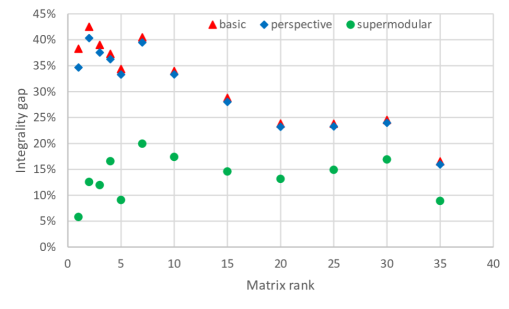
Figure 4. Integrality gap vs matrix rank ($\alpha=50$, $\delta=0.01$, $\rho=0$).

Finally, to evaluate the computational burden associated with the formulations, we plot in Figure 5 the time in seconds (in a logarithmic scale) require the solve the convex relaxations of each method for different dimensions $n$. Each point in Figure 5 corresponds to an average of 15 portfolio optimization instances generated with parameters $r=10$, $\delta=0.01$ and $\alpha\in\{2,10,50\}$ (5 instances for each value of $\alpha$). The time for Supermodular includes the total time used to generate cuts and solving the convex relaxations many times.

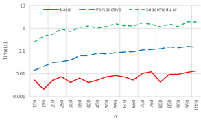
(a) General instances with $\rho=-1$.

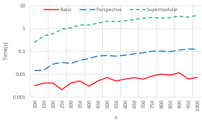
(b) Positive instances with $\rho=0$.

Figure 5. Solution time vs problem dimension ($r=10$, $\delta=0.01$).

We see that, in general, formulation Basic is an order-of-magnitude faster than Perspective, which in turn is an order-of-magnitude faster than Supermodular. Nonetheless, the computation times for Supermodular are adequate for many applications, solving instances with $n=1,000$ on average under four seconds.

Contrary to expectations, Supermodular is faster for general instances than for positive instances, despite the larger and more complex inequalities (28) used for the general case; for $n=1,000$, Supermodular runs in 1.9 seconds in general instances versus 3.8 seconds in positive instances. This counter-intuitive behavior is explained by the number of cuts added, as several more violated cuts are found in instances with large values of $\rho$, leading to larger convex formulations and the need to resolve them more times; for $n=1,000$, 20 cuts are added in each instance with $\rho=0$, whereas on average only 3.7 cuts are added in instances with $\rho=-1$.

The computation times are especially promising for tackling large-scale quadratic optimization problems with indicators, where alternatives to constructing strong convex relaxations (often based on decomposition of matrix $FF^{\prime}+D$ into lower-dimensional terms) may not scale. For example, Frangioni et al [26] solve convex relaxations of instances up to $n=50$, Han et al [33] solve relaxations for instances up to $n=150$, and Atamtürk and Gómez [6] report that solving the convex relaxation of quadratic instances with $n=200$ requires up to 1,000 seconds. All of these methods require adding $O(n^{2})$ variables and constraints to the formulations to achieve strengthening. In contrast, the supermodular inequalities (28) and (33) yield formulations with $O(nr)$ additional variables and constraints, which can be solved efficiently even if $n$ is large provided that the rank $r$ is sufficiently small: in our computations, instances with $r=10$ and $n=1,000$ are solved in under four seconds. Nonetheless, as discussed in the next section, even if the convex relaxations can be solved easily, incorporating the proposed convexification in branch-and-bound methods may required tailored implementations, not supported by current off-the-shelf branch-and-bound solvers.

6.4. On the performance with off-the-shelf branch-and-bound solvers

We also experimented with solving the formulations Supermodular obtained after adding cuts with CPLEX branch-and-bound algorithm. However, note that inequalities (28) and, to a lesser degree, inequalities (33), involve several ratios that can result in division by $0$ – from the proof of Proposition 10, we see that this in fact the case in many scenarios. Therefore, while we did not observe any particular numerical difficulties when solving the convex relaxations (via interior point methods), in a small subset of the instances we observed that the branch-and-bound method (based on linear outer approximations) resulted in numerical issues leading to incorrect solutions.

Table 5 reports the results on the two instances that exhibiting such pathological behavior. It shows, for each instance and method and different CPLEX settings, the bounds on the optimal solution obtained reported by CPLEX when solving the convex relaxation via interior point methods (barrier, corresponding to a lower bound), and lower and upper bounds reported by running the branch-and-bound algorithm for one hour. We do not scale the solutions obtained in Table 5. The tested settings are default CPLEX (def), default CPLEX with numerical emphasis enabled (+num), and CPLEX with numerical emphasis enabled and presolve and CPLEX cuts disabled (+num-pc).

Table 5. Examples of pathological behavior in branch-and-bound.

instance	method	setting	bounds
			barrier	lb_bb	ub_bb
	Perspective	def	0.0202	0.0942	0.0942
200-10-1.0-0.01	Supermodular	def	0.0243	0.1249	0.1249
-50.0-1-1-103†		+num	0.0243	0.1078	0.1078
		+num-pc	0.0243	0.0942	0.0942
	Perspective	def	0.1950	0.4849	0.4849
200-10-1.0-0	Supermodular	def	0.2471	0.4849	0.4849
-50.0-1-1-104††		+num	0.2471	0.4849	0.4849
		+num-pc	0.2471	0.5209	0.6629
$\dagger$ General portfolio instance with $\rho=-1$, $n=200$, $r=10$, $\delta=0.01$, $\alpha=50$
$\dagger\dagger$ General portfolio instance with $\rho=-1$, $n=200$, $r=10$, $\delta=0$, $\alpha=50$

In the first instance shown in Table 5, when using Supermodular with the default CPLEX settings, the solution reported is worse than the optimal solution by 30%. By enabling the numerical emphasis option, the solution improves but is still 10% worse than the solution reported by Perspective. Nonetheless, if presolve and CPLEX cuts are disabled, then both solutions coincide. The second instance shown in Table 5 exhibits the opposite behavior: when used with the default settings, independently of the numerical emphasis, the solutions obtained by Perspective and Supermodular coincide; however, if presolve and CPLEX cuts are disabled, then the lower bound obtained after one hour of branch-and-bound with the Supermodular method already precludes finding the correct solution. We point out that pathological behavior of conic quadratic branch-and-bound solvers have been observed in the past for other nonlinear mixed-integer problems with a large number of variables, see for example [6, 13, 26, 30].

7. Conclusions

In this paper we describe the convex hull of the epigraph of a rank-one quadratic functions with indicator variables. In order to do so, we first describe this convex hull of a underlying supermodular set function in a lower-dimensional space, and then maximally lift the resulting facets into nonlinear inequalities in the original space of variable. The approach is broadly applicable, as most of the existing results concerning convexifications of convex quadratic functions with indicator variables can be obtained in this way, as well as several well-known classes of facet-defining inequalities for mixed-integer linear problems.

Appendix A

Proof of Proposition 8.

In order to solve problem (25) we introduce an auxiliary variable $\gamma\in\mathbb{R}_{+}$ such that $\gamma=\max_{\alpha}(S^{+})$. Then, inequality (25) reduces to

$$t\geq\max_{S\subseteq N}\max_{\alpha,\gamma} -\frac{\gamma^{2}}{4}-\sum\limits_{i\in N\setminus S}\frac{\left(\alpha_{i}^{2}-\gamma^{2}\right)_{+}}{4}x_{i}+\alpha^{\prime}y$$ (38a)

s.t. $$\alpha_{i}\leq\gamma,\ \ i\in S$$ (38b)

$$\alpha\in\mathbb{R}_{+}^{N},\;\gamma\in\mathbb{R}_{+},$$ (38c)

where constraint (38b) enforces the definition of $\gamma$.

Note that there exists an optimal solution for (38) were $\gamma\leq\alpha_{i}$ for all $i\in N$: if $\alpha_{i}<\gamma$ for some $i\in N$, then setting $\alpha_{i}=\gamma$ yields a feasible solution with improved objective value. Therefore, $S$ is completely determined by $\gamma$ since $S=\left\{i\in N:\alpha_{i}\leq\gamma\right\}$.

Now, let $L=\left\{i\in N:\alpha_{i}=\gamma\right\}$ in a solution of (38). From the discussion above, we find that (38) reduces to

$$t\geq\max_{\alpha,\gamma}\; \gamma\cdot y(L)-\frac{\gamma^{2}}{4}\big{(}1-x(N\setminus L)\big{)}+\sum\limits_{i\in N\setminus L}\left(\alpha_{i}y_{i}-\frac{\alpha_{i}^{2}}{4}x_{i}\right)$$ (39a)

s.t. $$\gamma<\alpha_{i} \forall i\in N\setminus L$$ (39b)

$$\alpha\in\mathbb{R}^{N},\;\gamma\in\mathbb{R}_{+}.$$ (39c)

Observe that for $(L,\gamma)$ to correspond to an optimal solution, we require that $1-x(N\setminus L)\geq 0$ (otherwise $\gamma$ can be increased and set to an upper bound while improving the objective value). When this condition is satisfied, we find by taking derivatives of the objective and setting to 0, that $\alpha_{i}=2y_{i}/x_{i}$ for $i\in N\setminus L$ and $\gamma=2y(L)/\big{(}1-x(N\setminus L)\big{)}$, and (39) simplifies to (27). Note however that, in general, $(\alpha,\gamma)$ may not satisfy constraints (39b) for any choice of sets $L\subseteq N$. The constraints are satisfied if and only if $\gamma<\alpha_{i}$ for all $i\in N\setminus L$, i.e., if and only if conditions (26b) are satisfied.

In order for $L$ to be optimal we require condition (26c), i.e.,

$$\frac{y(L)}{1-x(N\setminus L)}\geq\frac{y_{i}}{x_{i}}.\quad\forall i\in L.$$

Indeed, if this condition is not satisfied for some $j\in L$, then increasing $\alpha_{j}$ from $\gamma=2\frac{y(L)}{1-x(N\setminus L)}\geq 2\frac{y_{j}}{x_{j}}$ to $2y_{j}/x_{j}$ (or setting it to $\beta$ if $\beta<2y_{j}/x_{j}$) results in a better objective value. ∎

References

- Ahmed and Atamtürk [2011] Ahmed S, Atamtürk A (2011) Maximizing a class of submodular utility functions. Mathematical programming 128(1-2):149–169
- Aktürk et al [2009] Aktürk MS, Atamtürk A, Gürel S (2009) A strong conic quadratic reformulation for machine-job assignment with controllable processing times. Operations Research Letters 37:187–191
- Alizadeh and Goldfarb [2003] Alizadeh F, Goldfarb D (2003) Second-order cone programming. Mathematical Programming 95:3–51
- Atamtürk [2001] Atamtürk A (2001) Flow pack facets of the single node fixed-charge flow polytope. Operations Research Letters 29:107–114
- Atamtürk and Bhardwaj [2015] Atamtürk A, Bhardwaj A (2015) Supermodular covering knapsack polytope. Discrete Optimization 18:74–86
- Atamtürk and Gómez [2018] Atamtürk A, Gómez A (2018) Strong formulations for quadratic optimization with M-matrices and indicator variables. Mathematical Programming 170:141–176
- Atamtürk and Gómez [2019] Atamtürk A, Gómez A (2019) Rank-one convexification for sparse regression. arXiv preprint arXiv:190110334
- Atamtürk and Gómez [2020] Atamtürk A, Gómez A (2020) Submodularity in conic quadratic mixed 0–1 optimization. Operations Research 68(2):609–630
- Atamtürk and Muñoz [2004] Atamtürk A, Muñoz JC (2004) A study of the lot-sizing polytope. Mathematical Programming 99:443–465
- Atamtürk and Narayanan [2020] Atamtürk A, Narayanan V (2020) Submodular function minimization and polarity. arXiv preprint arXiv:191213238 Forthcoming in Mathematical Programming
- Atamtürk et al [2001] Atamtürk A, Nemhauser GL, Savelsbergh MWP (2001) Valid inequalities for problems with additive variable upper bounds. Mathematical Programming 91:145–162
- Atamtürk et al [2017] Atamtürk A, Küçükyavuz S, Tezel B (2017) Path cover and path pack inequalities for the capacitated fixed-charge network flow problem. SIAM Journal on Optimization 27(3):1943–1976
- Atamtürk et al [2018] Atamtürk A, Gómez A, Han S (2018) Sparse and smooth signal estimation: Convexification of -formulations. arXiv preprint arXiv:181102655 Forthcoming in Journal of Machine Learning Research
- Bach [2019] Bach F (2019) Submodular functions: from discrete to continuous domains. Mathematical Programming 175:419–459
- Bertsimas and King [2015] Bertsimas D, King A (2015) Or forum—an algorithmic approach to linear regression. Operations Research 64:2–16
- Bienstock [1996] Bienstock D (1996) Computational study of a family of mixed-integer quadratic programming problems. Mathematical programming 74(2):121–140
- Bienstock and Michalka [2014] Bienstock D, Michalka A (2014) Cutting-planes for optimization of convex functions over nonconvex sets. SIAM Journal on Optimization 24:643–677
- Bonami et al [2015] Bonami P, Lodi A, Tramontani A, Wiese S (2015) On mathematical programming with indicator constraints. Mathematical Programming 151:191–223
- Ceria and Soares [1999] Ceria S, Soares J (1999) Convex programming for disjunctive convex optimization. Mathematical Programming 86:595–614
- Cozad et al [2015] Cozad A, Sahinidis NV, Miller DC (2015) A combined first-principles and data-driven approach to model building. Computers & Chemical Engineering 73:116–127
- Dong and Linderoth [2013] Dong H, Linderoth J (2013) On valid inequalities for quadratic programming with continuous variables and binary indicators. In: Goemans M, Correa J (eds) Proc. IPCO 2013, Springer, Berlin, pp 169–180
- Dong et al [2015] Dong H, Chen K, Linderoth J (2015) Regularization vs. relaxation: A conic optimization perspective of statistical variable selection. arXiv preprint arXiv:151006083
- Frangioni and Gentile [2006] Frangioni A, Gentile C (2006) Perspective cuts for a class of convex 0–1 mixed integer programs. Mathematical Programming 106:225–236
- Frangioni and Gentile [2007] Frangioni A, Gentile C (2007) SDP diagonalizations and perspective cuts for a class of nonseparable MIQP. Operations Research Letters 35:181–185
- Frangioni et al [2009] Frangioni A, Gentile C, Lacalandra F (2009) Tighter approximated MILP formulations for unit commitment problems. IEEE Transactions on Power Systems 24(1):105–113
- Frangioni et al [2020] Frangioni A, Gentile C, Hungerford J (2020) Decompositions of semidefinite matrices and the perspective reformulation of nonseparable quadratic programs. Mathematics of Operations Research 45(1):15–33
- Fujishige [2005] Fujishige S (2005) Submodular functions and optimization, vol 58. Elsevier
- Gómez [2018] Gómez A (2018) Submodularity and valid inequalities in nonlinear optimization with indicator variables
- Gómez [2019] Gómez A (2019) Outlier detection in time series via mixed-integer conic quadratic optimization. http://www.optimization-online.org/DB_HTML/2019/11/7488.html
- Gómez [2020] Gómez A (2020) Strong formulations for conic quadratic optimization with indicator variables. Forthcoming in Mathematical Programming
- Grötschel et al [1981] Grötschel M, Lovász L, Schrijver A (1981) The ellipsoid method and its consequences in combinatorial optimization. Combinatorica 1:169–197
- Günlük and Linderoth [2010] Günlük O, Linderoth J (2010) Perspective reformulations of mixed integer nonlinear programs with indicator variables. Mathematical Programming 124:183–205
- Han et al [2020] Han S, Gómez A, Atamtürk A (2020) 2x2 convexifications for convex quadratic optimization with indicator variables. arXiv preprint arXiv:200407448
- Hijazi et al [2012] Hijazi H, Bonami P, Cornuéjols G, Ouorou A (2012) Mixed-integer nonlinear programs featuring “on/off” constraints. Computational Optimization and Applications 52:537–558
- Jeon et al [2017] Jeon H, Linderoth J, Miller A (2017) Quadratic cone cutting surfaces for quadratic programs with on–off constraints. Discrete Optimization 24:32–50
- Kılınç-Karzan et al [2019] Kılınç-Karzan F, Küçükyavuz S, Lee D (2019) Joint chance-constrained programs and the intersection of mixing sets through a submodularity lens. arXiv preprint arXiv:191001353
- Lobo et al [1998] Lobo MS, Vandenberghe L, Boyd S, Lebret H (1998) Applications of second-order cone programming. Linear algebra and its applications 284:193–228
- Mahajan et al [2017] Mahajan A, Leyffer S, Linderoth J, Luedtke J, Munson T (2017) Minotaur: A mixed-integer nonlinear optimization toolkit. ANL/MCS-P8010-0817, Argonne National Lab
- Manzour et al [2019] Manzour H, Küçükyavuz S, Shojaie A (2019) Integer programming for learning directed acyclic graphs from continuous data. arXiv preprint arXiv:190410574
- Nemhauser and Wolsey [1988] Nemhauser GL, Wolsey LA (1988) Integer and Combinatorial Optimization. John Wiley & Sons
- Nemhauser et al [1978] Nemhauser GL, Wolsey LA, Fisher ML (1978) An analysis of approximations for maximizing submodular set functions – I. Mathematical Programming 14:265–294
- Nguyen et al [2018] Nguyen TT, Richard JPP, Tawarmalani M (2018) Deriving convex hulls through lifting and projection. Mathematical Programming 169(2):377–415
- Orlin [2009] Orlin JB (2009) A faster strongly polynomial time algorithm for submodular function minimization. Mathematical Programming 118:237–251
- Padberg et al [1985] Padberg MW, Van Roy TJ, Wolsey LA (1985) Valid linear inequalities for fixed charge problems. Operations Research 33(4):842–861
- Pochet [1988] Pochet Y (1988) Valid inequalities and separation for capacitated economic lot sizing. Operations Research Letters 7:109–115
- Richard and Tawarmalani [2010] Richard JPP, Tawarmalani M (2010) Lifting inequalities: a framework for generating strong cuts for nonlinear programs. Mathematical Programming 121:61–104
- Shi et al [2020] Shi X, Prokopyev OA, Zeng B (2020) Sequence independent lifting for the set of submodular maximization problem. In: International Conference on Integer Programming and Combinatorial Optimization, Springer, pp 378–390
- Tjandraatmadja et al [2020] Tjandraatmadja C, Anderson R, Huchette J, Ma W, Patel K, Vielma JP (2020) The convex relaxation barrier, revisited: Tightened single-neuron relaxations for neural network verification. arXiv preprint arXiv:200614076
- Van Roy and Wolsey [1986] Van Roy TJ, Wolsey LA (1986) Valid inequalities for mixed 0–1 programs. Discrete Applied Mathematics 14:199–213
- Wei et al [2020a] Wei L, Gómez A, Küçükyavuz S (2020a) Ideal formulations for constrained convex optimization problems with indicator variables. arXiv preprint arXiv:200700107
- Wei et al [2020b] Wei L, Gómez A, Küçükyavuz S (2020b) On the convexification of constrained quadratic optimization problems with indicator variables. In: International Conference on Integer Programming and Combinatorial Optimization, Springer, pp 433–447
- Wolsey [1989] Wolsey LA (1989) Submodularity and valid inequalities in capacitated fixed charge networks. Operations Research Letters 8:119–124
- Wu et al [2017] Wu B, Sun X, Li D, Zheng X (2017) Quadratic convex reformulations for semicontinuous quadratic programming. SIAM Journal on Optimization 27:1531–1553
- Wu and Küçükyavuz [2015] Wu HH, Küçükyavuz S (2015) Maximizing influence in social networks: A two-stage stochastic programming approach that exploits submodularity. arXiv preprint arXiv:151204180
- Xie and Deng [2020] Xie W, Deng X (2020) Scalable algorithms for the sparse ridge regression. SIAM Journal on Optimization 30:3359–3386
- Yu and Ahmed [2017a] Yu J, Ahmed S (2017a) Maximizing a class of submodular utility functions with constraints. Mathematical Programming 162(1-2):145–164
- Yu and Ahmed [2017b] Yu J, Ahmed S (2017b) Polyhedral results for a class of cardinality constrained submodular minimization problems. Discrete Optimization 24:87–102
- Yu and Küçükyavuz [2020] Yu Q, Küçükyavuz S (2020) A polyhedral approach to bisubmodular function minimization. arXiv preprint arXiv:200306036
- Zheng et al [2014] Zheng X, Sun X, Li D (2014) Improving the performance of MIQP solvers for quadratic programs with cardinality and minimum threshold constraints: A semidefinite program approach. INFORMS Journal on Computing 26:690–703