Growth, development, and structural change at the firm-level: The example of the PR China

Abstract

Understanding the microeconomic details of technological catch-up processes offers great potential for informing both innovation economics and development policy. We study the economic transition of the PR China from an agrarian country to a high-tech economy as one example for such a case. It is clear from past literature that rapidly rising productivity levels played a crucial role. However, the distribution of labor productivity in Chinese firms has not been comprehensively investigated and it remains an open question if this can be used to guide economic development. We analyze labor productivity and the dynamic change of labor productivity in firm-level data for the years 1998-2013 from the Chinese Industrial Enterprise Database. We demonstrate that both variables are conveniently modeled as Lévy alpha-stable distributions, provide parameter estimates and analyze dynamic changes to this distribution. We find that the productivity gains were not due to super-star firms, but due to a systematic shift of the entire distribution with otherwise mostly unchanged characteristics. We also found an emerging right-skew in the distribution of labor productivity change. While there are significant differences between the 31 provinces and autonomous regions of the P.R. China, we also show that there are systematic relations between micro-level and province-level variables. We conclude with some implications of these findings for development policy.

1 Introduction

For almost three decades, the PR China has been one of the fastest-growing economies. During this time, it made the transition from a largely agricultural developing country to the world’s second-largest industrial economy. Where state-owned enterprises (SOEs) ran the show in the 1980s, the country today is home to a multitude of private corporations of international importance. The PR China used to be a poor country and years behind in technological terms, but today, its development trajectory is of growing importance for the world in science and innovation, in CO2 emissions, and in technological impact on privacy, surveillance, and personal freedom. While the development is moderately well-understood in macro-economic terms, many open questions remain with regard to the development of the microstructure of the Chinese economy over the last decades. Which firms were the most productive ones, which were central to the transition process? How was productivity distributed among firms? How did this change over time? Can these processes be observed in all regions? In all sectors? Is it mirrored in profitability and investment rates? Can other developing economies achieve the same level of growth and development?

For developed countries, the distributions of firm-level data have been widely investigated and discussed in the literature. Many stylized facts are known although some questions remain contested. Ijiri and Simon (1964, 1977) proposed that firm sizes are highly skewed and follow Pareto distributions, essentially with a process following Gibrat’s law as the root cause of this. The observation was later confirmed with more detailed data sets (Axtell, 2001; Gaffeo et al., 2003), although some of the literature prefers to model the distribution as a lognormal (Cabral and Mata, 2003) and other generating algorithms have been proposed ((Heinrich and Dai, 2016) offer an overview). It is clear that this has important policy implications for competition law, innovation policy, labor market governance, and the effectiveness of policy interventions in industrial organization. Connections to firm growth, innovation, and technological change (Yu et al., 2015; Li and Rama, 2015) further add to the importance of this distributional approach, as do the later, but equally important investigations of the distributions of firm growth rates (Bottazzi and Secchi, 2006) and productivities (Yang et al., 2019).

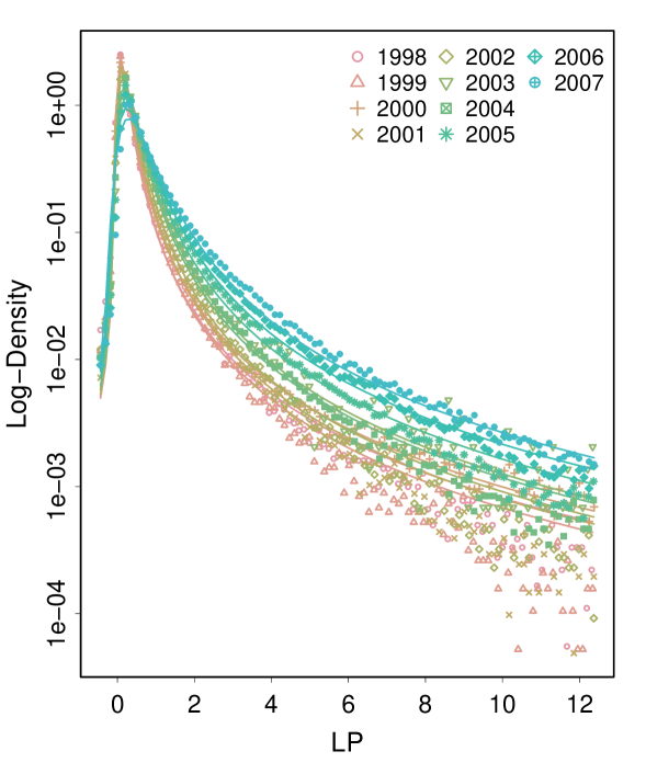
Figure 1: Density of the labor productivity ($LP$) distribution (full sample) by year in semi-log (vertical axis logarithmic). Solid lines indicate Levy alpha stable distribution fits as reported in Table 2.

An important characteristic of firm-level distributions in developed countries is that no significant changes are observed with either time (Yang et al., 2019) or firm age (Cabral and Mata, 2003). Developing countries, however, may be very different. They are subject to substantial and rapid changes in sectoral structure, technology, economic policy, and social organization. Investigating such distributional changes for developing economies may shed light on the mechanisms driving that development, the effectiveness of policy measures, the microstructural impact of technological change, as well as potentially the history of developed countries. Studying similar historical processes for developed countries would require older data that is almost certainly not available in high resolution.

For the PR China a look at the data immediately suggests that a systematic shift is underway: Figure 1 shows the distribution (density) function of the labor productivity at the firm-level by year in a semi-log plot (horizontal axis linear, vertical axis logarithmic); the shape of the distribution remains constant, but the right side (positive tail) moves outward and the peak becomes less pronounced. We will discuss other systematic shifts, interpretations, and implications below (see Section 5); for now, we emphasize that there are systematic changes in the distributional model during this development phase of the Chinese economy.

We use a firm-level data set for the PR China for the years 1998-2013 to investigate changes in the economic microstructure during the years of China’s most rapid growth from a distributional model perspective. We will focus on the distribution of labor productivity and of labor productivity change; these are arguably the quantities that are most closely related to economic development. While other distributional models have been suggested for labor productivity (Yu et al. (2015) consider Asymmetric Exponential Power (AEP) distributions and Gaussian normal distributions), the mounting evidence for heavy tails in both labor productivity and labor productivity change (Yang et al., 2019) suggests the Lévy alpha-stable distribution (Nolan, 1998, 2019) as a distributional model. Lévy alpha-stable distributions generalize Gaussian normal distributions, but have heavy tails for almost all parameter values.

Important consequences include that the apparent dispersion of labor productivity (Berlingieri et al., 2017) depends on how dispersion is measured. If such dispersion exists, it may be an indicator for misallocation of labor, capital, or other resources, a question of considerable relevance for the economy of the PR China (Hsieh and Klenow, 2009). It also relates to the debate on granular origins of aggregate fluctuations (Gabaix, 2011; Schwarzkopf et al., 2010) and the question of how characteristics of labor productivity distributions in firm populations should be quantified and interpreted. The characteristics of labor productivity dispersion measures and the consequences for these economic questions are studied comprehensively in Yang et al. (2019).

We demonstrate that labor productivity as well as labor productivity change and various other firm-level characteristics in the PR China are indeed fat-tailed with infinite variance. Further, we show that the Lévy alpha-stable distribution is an excellent fit and discuss how the characteristics of the distribution can be specified and tracked using the parameters of the Lévy alpha-stable fit. We discuss the emerging temporal and regional patterns as well as the behavior in other subsamples. Finally, we demonstrate connections between the distributions of labor productivity, labor productivity change, profitability, investment rate at the firm-level, as well as between these firm-level patterns and aggregated level data.

The paper is organized as follows: The literature on the development of productivity in the PR China during its period of rapid growth is reviewed in Section 2. Section 3 describes the data and the variables of interest. Section 4 discusses the distributional models that are tested, the Lévy alpha-stable and the Asymmetric Exponential Power, as well as the fitting procedure, and goodness of fit measures employed. Section 5 presents the findings and corresponding interpretations. Section 6 concludes.

2 Literature

The present paper aims to contribute to the study of distributional models of firm-level data, the investigation of the role of firm productivity in economic development, and, more specifically, the analysis of the rapid growth and development of the P.R. China in recent decades. We, therefore, give brief overviews of the literature in these three fields.

2.1 Distributional models of firm-level data

For developed countries, it has been established that the distributions of firm sizes, sales, etc. are heavily skewed (Ijiri and Simon, 1964; Axtell, 2001), with the Pareto (Axtell, 2001) and the lognormal distribution being proposed as distributional models (Cabral and Mata, 2003). The two-sided distributions of growth rates and productivities equally have much heavier tails than normal distributions; proposed distributional models include Asymmetric Exponential Power distributions for growth rates (Bottazzi and Secchi, 2006; Bottazzi et al., 2007; Bottazzi and Secchi, 2011) and Lévy alpha-stable distributions for productivities (Yang et al., 2019).

However, developed economies are relatively static. Very little change has been observed in these distributions over the recent decades for which good data is available (see e.g. (Yang et al., 2019)), and little change would be expected. To understand the development of firm-level distributions, scholars have instead focussed on firms of different age groups, their survival, and their shifts over time (Cabral and Mata, 2003). Important findings include that the form of the distribution does not change over time (Yang et al., 2019) or with age (Cabral and Mata, 2003; Angelini and Generale, 2008), that surviving firms are slightly larger (Cabral and Mata, 2003), and that they increase their productivity (making within-firm productivity gains important at the aggregate level) (Bartelsman et al., 2013; Li and Rama, 2015). Cabral and Mata (2003) report that surviving firms in a Portuguese data set have less long tails and lower skew; however, if the statistical process which the firm size follows in reality is heavy-tailed with low exponents, these moments may not exist and Cabral and Mata’s findings may be statistical artifacts (Yang et al., 2019). The hypothesis that small firms are more dynamic and account for significant shares of productivity gains and newly created jobs has frequently been proposed, but remains controversial (Li and Rama, 2015).

2.2 Economic development and firm-level productivity

Comprehensive firm-level data is often not available for developing countries. In turn, many studies have to work with small and potentially biased sample sizes. Notable exceptions are studies of firms in the P.R. China - using the Chinese Industrial Enterprise Database that we also work with - and in India - using government census data. While the general distributional forms found for developed countries are confirmed (Hsieh and Klenow, 2009; Ma et al., 2008; Zhang et al., 2009; Coad and Tamvada, 2012; Sun and Zhang, 2012; Yu et al., 2015; Ding et al., 2016; Heinrich and Dai, 2016), wider dispersions for productivities are reported for India and China specifically (Hsieh and Klenow, 2009).

In a general equilibrium interpretation, productivities should equalize, as investors should prefer high productivities while low productivity firms should be frozen out. This should be especially true for firms in the same sector and region, since portfolio diversification should not constitute a reason to invest in low productivity establishments. Of course, there may be structural reasons why investment in low productivity firms persists; and it might not be easily observable to investors. However, implications could still be drawn in comparative analyses, if different dispersions are observed. Hsieh and Klenow (2009) choose to follow this equilibrium interpretation; their contribution has led to the influential interpretation that resources are more misallocated in developing countries (Hsieh and Klenow, 2009; Song et al., 2011; Bartelsman et al., 2013; Li and Rama, 2015; Goyette and Gallipoli, 2015) as well as occasionally strongly worded policy recommendations (Adamopoulos and Restuccia, 2014; Poschke, 2018). This has been explained with both structural factors, such as constraints on credit availability (Bloom et al., 2010; Cabral and Mata, 2003), and also internal factors of the firm population of developing countries, such as bad management and reluctance to delegate decision-making (Bloom et al., 2010; Chaffai et al., 2012). More recently, it has been found that productivities (both labor productivity and total factor productivity, TFP) are heavy-tailed with tail exponents below $2.0$ such that most dispersion measures, including the ones used in this line of research, are not meaningful (Yang et al., 2019).

The source of productivity gains is an important question in the study of economic development. Three main causes are (1) within-firm improvements, (2) selection pressure (unproductive firms do not survive), and (3) changes from distributional differences between entrants and exiting firms. Within-firm improvements were particularly important in developing countries (Li and Rama, 2015) and in successful developing economies such as China (Yu et al., 2015, 2017). While developed countries show some component from selection (2) and entry/exit (3) (Fariñas and Ruano, 2004; Li and Rama, 2015), in some developing countries (Sub-Saharan Africa specifically) the entry-exit-process may come down to churning without any improvements, and firms may survive because they are born larger, not because they learn or improve (Van Biesebroeck, 2005; Li and Rama, 2015; Goyette and Gallipoli, 2015), resulting in heteroskedastic ”missing middle“ distributions (Van Biesebroeck, 2005).

Success and growth at the firm-level has been linked to innovation for Argentina (Chudnovsky et al., 2006), to innovation and technological competence for Indian firms (Coad and Tamvada, 2012), and export participation for Chilean, Chinese, and European firms (Volpe Martincus and Carballo, 2010; di Giovanni et al., 2011; Sun and Zhang, 2012).

Finally, systematic shifts in distributions have been shown for those developing countries that undergo rapid growth: Both Yu et al. (2015, 2017) and Ding et al. (2016) find a location shift in the productivity distributions (labor productivity and TFP respectively) for China in the 1990s and 2000s, indicating higher productivities across the entire firm population, while the functional form did not change. Nguyen (2019) finds a similar location shift in firm-level distributions for Vietnam. Heinrich and Dai (2016), studying the firm size distribution in Chinese provinces, find higher tail exponents in regions with high GDP per capita or high growth.

2.3 Firm-level productivity and growth in the PR China

Chinese firm-level distributions follow the same general patterns found elsewhere (Ma et al., 2008; Yu et al., 2015; Heinrich and Dai, 2016; Heinrich et al., 2020). While firm sizes seem to follow power laws (Ma et al., 2008; Heinrich and Dai, 2016), for labor productivities and growth rates, two distributions have been suggested: Asymmetric Exponential Power distributions from the exponential distribution family (Yu et al., 2015) were found to be a much better fit than Gaussians. Lévy alpha-stable distributions, which have power-law tails on both sides, have been suggested as an alternative since the data seems to be heavy-tailed (Heinrich et al., 2020). The distinction has important consequences.

The impressive economic growth of the PR China is reflected in the distributions as a location shift in productivity levels (Yu et al., 2015, 2017; Ding et al., 2016); the shift remains present in the gross industrial output per worker (labor productivity per wage), indicating that productivity has grown at a faster pace than labor inputs (Zhang and Liu, 2013). It is important to note that this is not a changing average, but a shift of the entire distribution which otherwise remains intact in spite of continuing entry and exit processes. The changes in the distribution’s parameters have so far not been comprehensively studied.

We give a brief overview over the contributing factors to China’s rapid growth from a historical perspective in Appendix C.

It this worthwhile to note that state-owned enterprises (SOEs) have been found to be in general less productive than privately owned firms, both in terms of average labor productivity and average TFP (Song et al., 2011; Yu et al., 2015; Hsieh and Song, 2015). While productivities of firms of all types vary widely and follow similar distributional forms as the economy as a whole (see Section 5), the mean difference is significant. SOE productivity did improve and has converged towards the productivity levels of private firms until at least 2007, but a gap in average productivity remains (Song et al., 2011; Yu et al., 2015). Boeing et al. (2016) find that compared to private firms, SOEs are less successful in converting patents into productivity improvements, although a generally positive relationship of productivity and R&D efforts does exist (Hu and Jefferson, 2004; Boeing et al., 2016). SOEs are often seen as a source of misallocation, thereby explaining their lower average productivity and tying the finding to the misallocation hypothesis (Hsieh and Klenow, 2009; Song et al., 2011). However, on the one hand, a closer look at the distributions reveals that the variation is still present within ownership type groups. On the other, firm-level dispersion may not be larger in China than in other countries if the measures employed in achieving these results were misleading for heavy-tailed data (Yang et al., 2019). The reason why SOEs are catching up and the mean difference between private firms and SOEs is converging is typically seen in the structural transformation of the state sector (Hsieh and Song, 2015; Jefferson et al., 2000). Greater flexibility of managers and delegation of decision-making capabilities as well as and the effects of rising incomes and autonomy on employee motivation have also been linked to the productivity improvements in SOEs (Groves et al., 1994).

Finally, regional disparities in productivity and other variables are well-known and expected for a country of the size of the PR China. Coastal provinces like Shanghai and Guangdong have a better TFP comparing with central and western provinces (Ding et al., 2016; Chen et al., 2009). High productivity firms prefer to concentrate their activities on regions with developed infrastructure, good universities, and related industrial clusters; Zhu et al. (2019) finds evidence for both sorting and adverse sorting effects. Meanwhile, officials in undeveloped regions are eager to attract investment by providing subsidies. However, government subsidies may attract low-productivity firms, since they have low opportunity costs (Zhu et al., 2019). Marshall and Jacobs externalities of spatial industrial agglomerations (Beaudry and Schiffauerova, 2009) likely also play a role in creating and maintaining regional disparities, as may the openness of regions towards outside influences, foreign trade, and flexible economic policy (Jiang, 2011).

3 Data

3.1 Sources

We use firm-level data from the Chinese Industrial Enterprise Database (CIEDB), which records several hundreds of thousands of firms each year for the time period between 1998 and 2013 and is commonly used by researchers working on firm-level data in China (Brandt et al., 2012; Hsieh and Song, 2015; Ding et al., 2016; Yu et al., 2015, 2017). The data ultimately derive from data recorded by the PR China’s National Bureau of Statistics. Similar to data provided by the Bureau van Dijk for Europe (ORBIS Europe), the CIEDB records data at the firm-level, not at the level of physical entities (plants). This facilitates investigating structural characteristics such as productivity and profitability at the firm-level, the level at which decision making and management take place. Different from other databases like COMPUSTAT or Bloomberg, but similar to ORBIS Europe, the CIEDB also includes small and medium-sized firms and thus provides better coverage of different types of enterprises. The data set also records the ownership type (state-owned, foreign-owned, private, etc.).

There are some notable difficulties with the data, especially for the period after 2008. These difficulties are well-known and recognized in the literature (Brandt et al., 2014). Brandt et al. (2014) qualify the samples after 2008 as unreliable and recommend working with the more reliable date up to 2008 only. We largely follow this strategy. We complement this with later data from the period 2009-2013, where possible, to shed light on some developments after 2008.

Up to 2008, the database includes industrial firms with revenues above $5$ million Yuan. From 2009, only firms with revenues beyond $20$ million Yuan are present in the data set. The set of recorded variables also changes significantly over this time period. For instance, we are unable to compute value-added and productivities for the time period after 2008, as the measures required for their computation are only reported up until 2007.

In addition, we use industry level deflators from and macroeconomic data at province level from China Compendium of Statistics (1949-2008).

3.2 Data processing

We extract variables on identity (ID, phone number, ZIP code), characteristics (founding year, primary sector, ownership type), and structural and financial condition (output, assets, profits, wages, employment, intermediate input). These variables are present in the database throughout the years 1998-2007. Progressively more variables either missing or reported in substantially different form starting in 2008. (See Table 1.) The monetary variables are deflated using industry level deflators.

We remove duplicates in terms of ID and Year before commencing with the data analysis.

In order to observe productivity changes, we attempt to identify firms that are present over multiple years both directly (using the unique ID) and indirectly, using phone numbers and address details as suggested in Brandt et al. (2014).

For the analysis of regional variation, the firms are assigned to the region of their postal address. As the region name is not typically part of the postal address, the ZIP codes were used to identify those regions.

Year	Labor productivity	Labor productivity change	Labor productivity growth	Labor productivity (imputed)	Profitability	Investment rate
1998	141,790	-	-	141,787	149,270	-
1999	148,982	113,684	112,996	148,973	147,636	121,091
2000	147,196	121,977	120,882	147,188	148,088	123,492
2001	158,671	116,674	116,001	158,664	157,453	119,211
2002	169,419	139,020	138,351	169,417	168,072	137,724
2003	11,404	9,503	9,490	11,404	11,369	9,461
2004	267,898	120,595	120,174	267,898	263,060	118,202
2005	262,830	227,569	227,032	262,830	261,369	223,671
2006	290,762	244,918	244,406	290,762	289,566	243,448
2007	324,638	268,614	268,376	324,638	323,131	267,151
2008	-	-	-	-	198,945	158,114
2009	-	-	-	-	-	130,155
2010	-	-	-	-	-	152,979
2011	-	-	-	-	-	-
2012	-	-	-	42,301	-	36,139
2013	-	-	-	41,625	216,817	180,634

Table 1: Number of observations per variable and year after cleaning.

3.3 Variables

In order to investigate structural change at the firm-level, we analyze labor productivity and its dispersion and dynamical change. Labor productivity has been conjectured to hold information about the firm’s capabilities, economic potential, and growth prospects. Its dynamical change facilitates investigating to what extent this potential is persistent in time. The dispersion of both variables holds information on the structural composition of the firm population of the country, the region, or the industry.

Labor productivity is defined as value-added per employee.

$$LP_{i,t}=VA_{i,t}/L_{i,t}$$

where $i$ indicates the firms and $t$ is the time. As the value-added is not part of the database, it has to be computed as the difference between output and intermediate input.

$$VA_{i,t}=Q_{i,t}-II_{i,t}$$

where $Q_{i,t}$ is output and $II_{i,t}$ stands for intermediate input of firm $i$ at time $t$. Alternatively, $VA$ can be imputed as the sum of paid wages $W_{i,t}$ and profits $\Pi_{i,t}$

$$\widetilde{VA}_{i,t}=W_{i,t}+\Pi_{i,t}.$$

Imputed value-added differs from the direct computation in that reinvestments cannot be distinguished from negative profits and remain part of the resulting quantity. Reinvestments can be substantial and may occur in systematic patterns across the firm population.

To observe the dynamic development of labor productivities, we compute the labor productivity change by firm

$$\Delta LP_{i,t}=LP_{i,t}-LP_{i,t-1}.$$

An alternative choice would be labor productivity growth

$$\dot{LP}_{i,t}=\frac{LP_{i,t}-LP_{i,t-1}}{LP_{i,t-1}}.$$

However, as this is a growth rate, it has a singularity at $LP_{i,t-1}=0$. Changes in labor productivity in the vicinity of the singularity get grotesquely exaggerated. What is more, $LP_{i,t}$ may be zero (in 1% of the observations) or negative (3% of the observations) since stocks and price changes are allowed. For this reason, we refrain from using the growth rate and rely on the absolute change $\Delta LP_{i,t}$ as our main indicator of the dynamical change of labor productivities.

The distributional models for these variables will be investigated in Section 5.1. It will be shown that this has important consequences for the selection and interpretation of quantitative measures for productivity dispersion. We complement the analysis of labor productivity with the study of the behavior of and dispersion of two more variables: Return on capital will serve as an indicator for the firms’ profitability from the perspective of investors. The investment rate is studied to assess investment patterns and growth. These variables are computed as

$$ROC_{i,t}=\frac{\Pi_{i,t}}{K_{i,t}}$$

$$IR_{i,t}=\frac{K_{i,t}-K_{i,t-1}}{K_{i,t-1}}$$

where $\Pi_{i,t}$ are the profits and $K_{i,t}$ is the capital stock (fixed assets) of firm $i$ at time $t$.

The number of observations for all variables by year is given in Table 1.

Additional analyses also use capital intensity, defined as:

$$CI_{i,t}=K_{i,t}/L_{i,t}$$

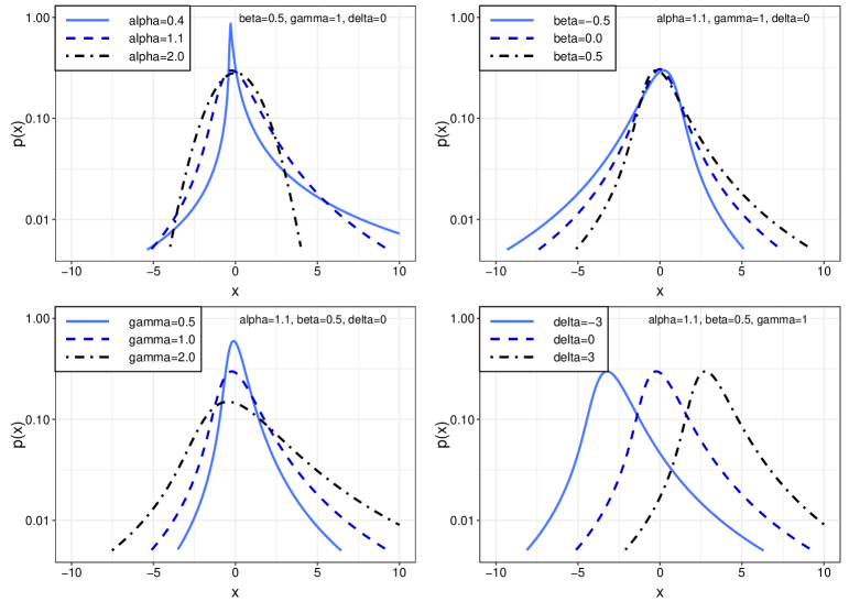
Figure 2: Density of the Lévy alpha-stable distribution for different parameter settings. Upper left: Variation of tail parameter $\alpha$. Upper right: Variation of skew parameter $\beta$. Lower left: Variation of scale parameter $\gamma$. Lower right: Variation of location parameter $\delta$.

4 Methods

4.1 Distributional models

Most studies of labor productivity and of firm-level data, in general, are based on generative models. They define, which effects on the measure under investigation are considered under the model; they fix their functional forms; and they establish the resulting distribution. Typically, the approximate form of the distribution to be explained is known, which constrains the variety of candidate models.

The advantages of the generative approach include that it is illustrative and verifiable by considering other quantities represented in the model. However, specific distributions can frequently be generated by large numbers of different generative models, and matching the correct distribution reveals little information about the correct generating process.

Instead, and in line with much of the modern literature (Frank, 2009; Bottazzi and Secchi, 2006; Yang, 2018; Yang et al., 2019), we consider a different approach: The attractor distribution to which the result of aggregations of (identical, independent) distributions converges. We remain agnostic with regard to the interpretation of the component distributions being aggregated, though temporal aggregation of shocks or aggregation across jobs, processes, or tasks within a firm are natural component separations that suggest themselves. If it is indeed the correct representation of the data, the distribution could be expected to remain stable under a number of changes to the system, as the aggregation continues to converge to this functional form.

In particular, following Yang et al. (2019), we use the Lévy alpha-stable distribution (Nolan, 2019, 1998) as our main distributional model, although we provide fits to the 4-parameter Asymmetric Exponential Power distribution suggested elsewhere in the literature (Bottazzi and Secchi, 2006; Bottazzi et al., 2007; Bottazzi and Secchi, 2011; Yu et al., 2015) as a point of comparison. In the following, we provide a non-technical explanation and some intuition why the Lévy alpha-stable distribution may be a good distributional model. A technical description is given in the Appendix A.

Random variables distributions can be aggregated in convolutions (i.e. summation of the variables), which yields a different distribution of the results (for technical details, see Appendix A.1). Aggregation leads to a loss of information; it washes out less strong signals and only a dominant pattern remains. As the convoluted distributions are independent, this pattern is the one that carries the least information (highest entropy), the one that is the most likely one without additional information, the one that constitutes the maximum entropy distribution under constraints that depend on the component distributions $X$.

The maximum entropy perspective may be helpful in that it allows computing the resulting distribution and understanding the type of its constraints in a concise way. The resulting distributional form is determined by the constraints in the maximum entropy perspective, or equivalently by the type of convolution and the characteristics of the component distributions in the convolution perspective. For instance, a single constraint on the mean of the distribution will yield an exponential or Laplacian (two-sided exponential) maximum entropy distribution. The Asymmetric Exponential Power distributions that are often used for the distributional models for firm growth (Bottazzi and Secchi, 2006; Bottazzi et al., 2007; Bottazzi and Secchi, 2011) or productivity (Yu et al., 2015), belong to this family, albeit with a modification that allows for asymmetry (for technical details, see Appendix A.5). A single constraint on the mean of the distribution under logarithmic transformation will yield a Pareto maximum entropy distribution, typically considered for distributional models of firm size distributions. A constraint on the variance of a distribution (implying a second constraint on the mean) will yield a Gaussian normal maximum entropy distribution.

Almost all maximum entropy distributions do not constitute attractors under further aggregation. If the resulting distribution is further convoluted, it continues to change. Those that do constitute attractors, i.e. those that yield an identical distribution under convolution are known as Lévy alpha-stable distributions (for technical details, see Appendix A.4). The Lévy alpha-stable is a generalization of several families of distributions, including Gaussian normal distributions, Cauchy, distributions and Lévy distributions. The generalized central limit theorem (GCLT) states that any sum of independent, identical distributions will converge to a Lévy alpha-stable distribution. Specifically, if the convoluted distributions have a finite variance, the sum will converge to a Gaussian normal, a member of the family of Lévy alpha-stable distributions (for technical details, see Appendix A.2). If not, it will yield a different member of this family with a heavy tail and a tail parameter $<2$.

Lévy alpha-stable distributions do not have a closed-form representation as a function in the frequency domain, except for special parameter sets. The functional form in the Fourier domain (the characteristic function, for technical details, see Appendix A.3) is

$$\varphi(s)=\operatorname{E}[e^{(isx)}]={\begin{cases}e^{(-\gamma^{\alpha}|s|^{\alpha}[1+i\beta\text{tan}\left({\tfrac{\pi\alpha}{2}}\right)\operatorname{sgn}(s)\left((\gamma|s|)^{1-\alpha}-1\right))]+i\delta s)}&\alpha\neq 1\\ e^{(-\gamma|s|[1+i\beta{\tfrac{2}{\pi}}\operatorname{sgn}(s)\log(\gamma|s|)]+i\delta s)}&\alpha=1\end{cases}}$$ (1)

Figure 2 shows the bahaviour of the four parameters of the Lévy alpha-stable distribution in semi-log scale (y-axis logarithmic). The upper left panel contrasts the Gaussian case (black curve) with skewed fat-tailed cases for different tail indices $\alpha$. Note that the curve bends outward for the two fat-tailed cases, indicating that the tails are heavier than in an exponential distribution, which would be linear in a semi-log scale. This is a tell-tale sign of fat-tailedness. The lower left panel shows variations of the scale or width of the distribution. The scale, $\gamma$ is another measure of dispersion besides the tail index and is independent from it. In the Gaussian case ($\alpha=2$), the scale is simply the standard deviation. For fat-tailed variants ($\alpha<2$) such as the ones depicted in this panel, this is not the case, as the standard deviation is infinite. The right panels demonstrate different skew values and a location shift respectively.

More technical details on Lévy alpha-stable distributions can be found in Nolan (1998, 2019); a comprehensive discussion of maximum entropy, aggregation of distributions, and characteristic equations in the Fourier domain is offered in Frank (2009).

4.2 Fitting

4.2.1 Lévy alpha-stable distributions

We use Nolan’s (Nolan, 1998, 2019) parametrization $0$ for the Lévy alpha-stable distribution as given in equation 1. Common methods to fit the distribution include maximum likelihood, the general method of moments (GMM), and McCulloch’s (McCulloch, 1986) quantile based estimation. Maximum likelihood is generally considered the most reliable, but requires much more computation power than the alternatives and is, for the data sizes considered here, not practical. A direct comparison of McCulloch’s method with GMM showed that for the relevant data sizes of at least $1000$, $5000$, and $10000$ (depending on the type of the subsample, see Section 3) observations each as considered here, McCulloch’s quantile-based estimation is more accurate and gives generally better Soofi ID scores (see Section4.3.1).

We use the R package StableEstim (Kharrat and Boshnakov, 2016).

4.2.2 Asymmetric exponential power (AEP) distributions

Contrasting our distributional model to AEP distributions is expedient not only because it has been suggested as a distributional model in the literature (Bottazzi and Secchi, 2006; Bottazzi et al., 2007; Bottazzi and Secchi, 2011; Yu et al., 2015), but also because AEP distributions show radically different tail behavior compared to Lévy alpha-stable distributions, which are heavy-tailed and have infinite variance for $\alpha<2$. While finite samples always have a finite variance, it will diverge in the sample size if the underlying distribution of the sample is heavy-tailed. As a result, measuring the variance of a sample from a heavy-tailed distribution will yield misleading results (Nolan, 2019; Emberchts et al., 1997; Yang et al., 2019), as they are tainted by other quantities such as the sample size. Similar problems exist for other dispersion measures (Yang et al., 2019). Performing OLS correlations on variables with hevy tails will likely also fail, since the error distribution will likely inherit the heavy tails and OLS requires errors with finite variance. For technical details, see Appendix A.6.

We use a 4-parameter AEP distribution with the functional form given in equation 22 as an alternative distributional model for comparison. Fitting relies on the L-moments method as discussed in Asquith (2014) and implemented in the R package lmomco (Asquith, 2018).

4.3 Goodness of fit

Two measures for model selection and validation are used, both based on information theory considerations. Additional techniques, such as the Kolmogorov-Smirnov test or cross-validation are possible, but were not applied in the present study.

4.3.1 Soofi ID index

Our main goodness-of-fit metric is based on Soofi et al.’s (Soofi et al., 1995) information distinguishability ($ID$) concept, which gives the distinguishability of two distributions based on their information content. We can use this measure to assess to what extent a fitted model $p(\theta|x)$ with parameters $\theta$ is distinguishable from the entropy maximizing distribution $q(\theta|x)$ given a set of observations $x$.

Formally, $ID$ is based on the Kullback-Leibler divergence between the two distributions

$$D_{\mathrm{KL}}(p\|q)=\sum_{i}p(x_{i})\,\log{\frac{p(x_{i})}{q(x_{i})}},$$

where $\|$ is the divergence operator. Information distinguishability is defined as

$$ID(p\|q|\theta)=\exp[-D_{\mathrm{KL}}(p\|q|\theta)],$$ (2)

and has support $ID\in[0,1]$. $ID=0$ indicates that the distributions are indistinguishable, while the differences are more pronounced the higher $ID$. For convenience, we construct a Soofi ID score $SIDS$ as previously used by Yang (2018); Yang et al. (2019) by rescaling $ID$

$$SIDS=100\times(1-ID),$$ (3)

with support $SIDS\in[0,100]$ such that $SIDS=100$ indicates a perfect match while low values indicate that the distributional model under investigation is probably not correct for the sample in question.

4.3.2 Akaike information criterion (AIC)

Akaike’s (Akaike, 1973) information criterion (AIC) is based on the likelihood of a distributional model fit while accounting for the number of parameters. Formally,

$$\operatorname{AIC}=2k-2\log\mathcal{L}(\theta|x)$$ (4)

where $\mathcal{L}(\theta|x)$ is the likelihood function of parameters $\theta$ given data $x$ and $k$ is the number of estimated parameters $\theta$.

The AIC relies on the same concepts as the $SIDS$, namely minimizing Kullback-Leibler divergence, but rescales differently and applies a correction for $k$. It offers a measure for model comparison, but is difficult to interpret in illustrative terms. $SIDS$, on the other hand, has a straight forward interpretation as the extent of similarity with an entropy maximizing model given the data.

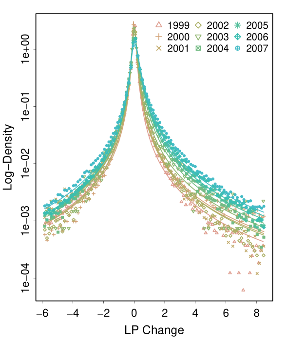
Figure 3: Density of the labor productivity change ($\Delta LP$) distribution (full sample) by year in semi-log (vertical axis logarithmic). Solid lines indicate Levy alpha stable distribution fits as reported in Table 2.

	Year	$\#$Obs.	Lévy alpha-stable fit				AEP fit
			$\alpha$	$\beta$	$\gamma$	$\delta$	$\kappa$	$h$	$\sigma$	$\xi$
LP	1998	140,372	1.00	0.95	0.11	0.11	0.47	0.40	0.01	0.06
	1999	147,492	1.06	0.95	0.12	0.13	0.45	0.46	0.02	0.07
	2000	145,724	0.97	0.95	0.14	0.14	0.42	0.27	0.00	0.10
	2001	157,083	1.08	0.95	0.15	0.18	0.42	0.48	0.02	0.10
	2002	167,723	1.08	0.95	0.17	0.20	0.44	0.48	0.03	0.12
	2003	11,288	1.04	0.95	0.21	0.28	0.43	0.40	0.02	0.18
	2004	265,218	1.06	0.95	0.20	0.25	0.42	0.45	0.03	0.15
	2005	260,200	1.03	0.95	0.25	0.30	0.40	0.45	0.03	0.17
	2006	287,854	1.00	0.95	0.30	0.36	0.37	0.43	0.03	0.21
	2007	321,390	0.99	0.95	0.36	0.43	0.36	0.43	0.03	0.24
$\Delta LP$	1999	112,546	0.96	-0.05	0.08	0.01	1.07	0.34	0.00	0.02
	2000	120,757	0.90	0.25	0.09	-0.00	0.72	0.22	0.00	-0.04
	2001	115,506	0.93	-0.11	0.10	0.01	1.28	0.24	0.00	0.07
	2002	137,628	0.99	0.12	0.11	0.01	0.92	0.41	0.02	0.01
	2003	9,407	0.97	0.14	0.13	0.01	0.90	0.38	0.01	0.00
	2004	119,389	1.03	0.20	0.18	0.02	0.86	0.42	0.03	0.00
	2005	225,293	1.01	0.26	0.19	0.04	0.84	0.42	0.03	0.02
	2006	242,468	0.99	0.29	0.20	0.05	0.81	0.40	0.03	0.02
	2007	265,926	0.99	0.25	0.25	0.06	0.84	0.40	0.03	0.04
$ROC$	1998	136,435	0.91	0.37	0.08	0.00	0.73	0.34	0.00	-0.01
	1999	145,513	0.91	0.44	0.07	0.00	0.69	0.34	0.00	-0.01
	2000	141,570	0.93	0.51	0.08	0.01	0.67	0.34	0.00	-0.00
	2001	155,527	0.93	0.55	0.09	0.02	0.65	0.32	0.00	0.00
	2002	166,246	0.98	0.61	0.10	0.03	0.64	0.34	0.00	0.01
	2003	11,250	1.01	0.59	0.11	0.05	0.65	0.36	0.01	0.03
	2004	260,311	0.96	0.61	0.12	0.05	0.63	0.31	0.00	0.02
	2005	258,741	1.00	0.69	0.14	0.06	0.59	0.35	0.01	0.02
	2006	286,602	1.01	0.78	0.14	0.06	0.56	0.35	0.01	0.03
	2007	319,847	1.02	0.92	0.15	0.07	0.52	0.35	0.01	0.03
	2012	40,840	1.00	0.75	0.18	0.09	0.55	0.36	0.01	0.03
	2013	40,090	0.96	0.74	0.18	0.09	0.55	0.33	0.01	0.04
$IR$	1999	119,401	0.86	0.40	0.09	-0.04	0.61	0.24	0.00	-0.09
	2000	118,108	0.86	0.40	0.09	-0.06	0.61	0.25	0.00	-0.12
	2001	117,732	0.86	0.41	0.10	-0.02	0.60	0.25	0.00	-0.09
	2002	136,224	0.84	0.46	0.11	-0.02	0.57	0.24	0.00	-0.08
	2003	9,362	0.93	0.58	0.13	-0.05	0.53	0.23	0.00	-0.10
	2004	116,966	0.92	0.66	0.24	-0.12	0.49	0.26	0.00	-0.22
	2005	221,420	0.82	0.60	0.15	-0.02	0.49	0.23	0.00	-0.09
	2006	240,962	0.87	0.58	0.14	-0.03	0.53	0.25	0.00	-0.09
	2007	264,428	0.86	0.59	0.14	-0.04	0.52	0.25	0.00	-0.11
	2008	156,516	0.78	0.59	0.15	-0.07	0.48	0.22	0.00	-0.16
	2009	128,846	0.87	0.56	0.18	0.02	0.53	0.25	0.00	-0.07
	2010	151,441	0.63	0.20	0.03	-0.03	0.51	0.10	0.00	-0.10
	2012	8,746	0.88	0.95	0.58	-0.03	0.36	0.25	0.00	-0.22
	2013	35,452	0.86	0.55	0.11	-0.05	0.54	0.22	0.00	-0.10

Table 2: Lévy alpha-stable and AEP parameter fits for labor productivity $LP$, labor productivity change $\Delta LP$, profitability $ROC$, and investment rate $IR$ by year. Fits with comparatively better goodness in either $SIDS$ or $AIC$ in bold, provided $SIDS>95$. Details of the associated goodness of the fits are given in Table 3.

	Year	Lévy alpha-stable		AEP		$\Delta SIDS$	$\Delta AIC$	Preferred model
		$SIDS$	$AIC$	$SIDS$	$AIC$
$LP$	1998	98.78	880.11	88.71	913.49	10.07	-33.38	Lévy $\alpha$-s.
	1999	98.10	803.04	93.86	845.21	4.24	-42.17	Lévy $\alpha$-s.
	2000	99.76	1,249.25	99.14	1,320.87	0.62	-71.61	Lévy $\alpha$-s.
	2001	98.26	797.22	94.86	843.04	3.40	-45.82	Lévy $\alpha$-s.
	2002	98.43	826.50	94.88	859.14	3.55	-32.64	Lévy $\alpha$-s.
	2003	98.78	979.66	83.90	1,023.38	14.88	-43.72	Lévy $\alpha$-s.
	2004	98.45	884.45	95.01	927.27	3.44	-42.82	Lévy $\alpha$-s.
	2005	97.88	923.83	94.10	975.49	3.78	-51.66	Lévy $\alpha$-s.
	2006	97.49	972.51	93.41	1,025.50	4.08	-52.99	Lévy $\alpha$-s.
	2007	96.75	1,012.76	95.21	1,071.37	1.54	-58.61	Lévy $\alpha$-s.
$\Delta LP$	1999	99.35	914.08	95.89	937.44	3.46	-23.36	Lévy $\alpha$-s.
	2000	94.48	1,322.04	94.48	1,357.34	0.00	-35.30	-
	2001	97.92	1,301.04	84.58	1,337.90	13.34	-36.87	Lévy $\alpha$-s.
	2002	99.22	824.87	98.95	852.95	0.27	-28.09	Lévy $\alpha$-s.
	2003	98.96	901.36	98.85	931.11	0.11	-29.75	Lévy $\alpha$-s.
	2004	99.12	908.20	96.55	929.40	2.57	-21.20	Lévy $\alpha$-s.
	2005	99.22	925.94	99.56	948.58	-0.34	-22.64	Lévy $\alpha$-s.
	2006	99.14	965.16	99.53	989.38	-0.39	-24.22	Lévy $\alpha$-s.
	2007	99.24	1,003.31	99.33	1,024.51	-0.09	-21.20	Lévy $\alpha$-s.
$ROC$	1998	92.99	919.04	96.53	960.82	-3.54	-41.78	AEP
	1999	98.53	899.66	91.12	934.49	7.41	-34.83	Lévy $\alpha$-s.
	2000	98.86	920.60	99.79	961.19	-0.93	-40.60	even
	2001	98.38	978.17	96.66	1,018.65	1.72	-40.48	Lévy $\alpha$-s.
	2002	99.06	973.09	99.11	1,017.00	-0.05	-43.92	even
	2003	98.85	911.05	96.70	939.00	2.15	-27.95	Lévy $\alpha$-s.
	2004	99.55	1,067.32	97.29	1,110.23	2.26	-42.91	Lévy $\alpha$-s.
	2005	98.16	1,003.81	99.50	1,038.32	-1.34	-34.52	even
	2006	97.26	1,016.92	99.15	1,047.34	-1.89	-30.41	even
	2007	95.28	1,062.73	97.86	1,072.13	-2.58	-9.41	even
	2012	95.20	1,031.04	97.74	1,060.46	-2.54	-29.43	even
	2013	96.63	1,063.87	94.74	1,095.59	1.89	-31.72	Lévy $\alpha$-s.
$IR$	1999	98.54	1,230.72	94.70	1,277.72	3.84	-47.00	Lévy $\alpha$-s.
	2000	98.27	1,221.62	94.69	1,283.48	3.58	-61.86	Lévy $\alpha$-s.
	2001	95.30	1,243.37	90.81	1,293.24	4.49	-49.88	Lévy $\alpha$-s.
	2002	96.57	1,243.78	96.28	1,296.99	0.29	-53.21	Lévy $\alpha$-s.
	2003	96.10	1,419.75	96.05	1,481.73	0.05	-61.98	Lévy $\alpha$-s.
	2004	95.63	1,408.22	93.21	1,475.98	2.42	-67.76	Lévy $\alpha$-s.
	2005	94.48	1,350.69	85.73	1,408.57	8.75	-57.88	-
	2006	97.43	1,263.57	90.15	1,308.09	7.28	-44.52	Lévy $\alpha$-s.
	2007	97.06	1,239.16	79.77	1,283.18	17.29	-44.02	Lévy $\alpha$-s.
	2008	96.17	1,373.84	92.12	1,428.20	4.05	-54.35	Lévy $\alpha$-s.
	2009	97.73	1,302.20	94.31	1,351.16	3.42	-48.96	Lévy $\alpha$-s.
	2010	88.00	1,786.06	77.35	1,810.14	10.65	-24.09	-
	2012	98.39	1,508.08	81.76	1,565.72	16.63	-57.64	Lévy $\alpha$-s.
	2013	95.42	1,297.17	90.06	1,342.75	5.36	-45.57	Lévy $\alpha$-s.

Table 3: Goodness of fit measures for Lévy alpha-stable and AEP parameter fits for labor productivity $LP$, labor productivity change $\Delta LP$, profitability $ROC$, and investment rate $IR$ by year as reported in Table 2. The last column notes the fit with comparatively better goodness in either $SIDS$ or $AIC$ in bold, provided $SIDS>95$.

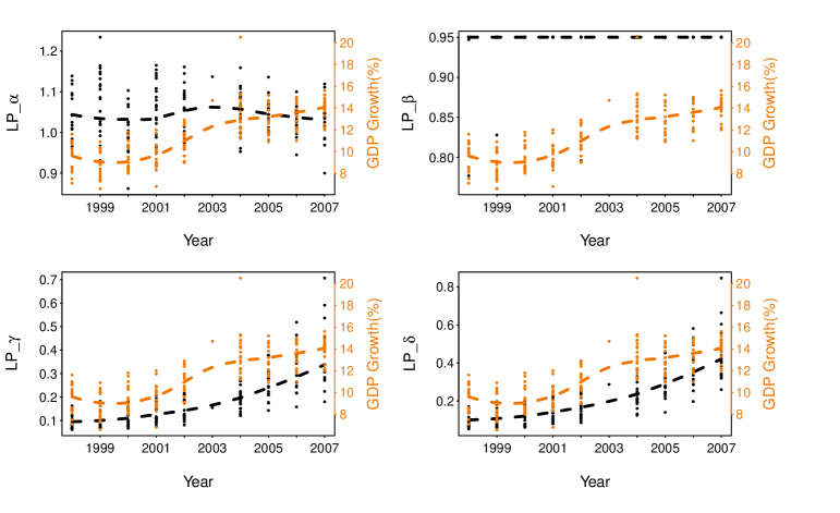
Figure 4: $LP$ (labor productivity) by region and year (black) in comparison to GDP growth (orange).

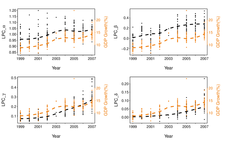
Figure 5: $\Delta LP$ (labor productivity change) by region and year (black) in comparison to GDP growth (orange).

5 Results

In this section, we investigate questions that are of importance for understanding developing economies in general and the Chinese case during the decade of rapid catch-up (1999-2013, the period for which we have data) in particular.

1. What distributional model should be used for productivity microdata for developing countries (here, the P.R. China)? Do they differ from developed countries? (Section 5.1)

2. Do the parameters of these distributions change with advancing development level? (Section 5.2)

3. Are there persistent differences between regions (or countries)? (Section 5.3)

4. If there are any systematic differences or developments, how do they relate to other characteristics at the micro- or macro-level (firm age, GDP growth, capital intensity, employment)? (Section 5.4)

Although our analysis is limited to the P.R. China, we can draw comparisons to the distributions of firm-level productivity data for developed economies (Yang et al., 2019) and conjecture that other developing economies may show similar patterns in phases of rapid economic catch-up. We also leverage the considerable diversity between Chinese provinces to assess regional differences, which may be an indicator of how different developing countries should be expected to be from one another in this regard.

5.1 Fitting productivity distributions

We performed parameter fits with the Lévy alpha-stable model and, as a point of comparison, for the AEP model for all variables listed in section 3.3. However, we concentrate our analysis on the labor productivity $LP$, and the labor productivity change $\Delta LP$, while the other variables ($ROC$, $IR$) serve as a point of comparison and to show that the functional forms of the distributions are connected. Lévy alpha-stable fit lines as well as empirical density by year are shown in Figures 1 ($LP$) and 3 ($\Delta LP$). The parameter values for the fits are given in the upper two sections of Table 2, while the goodness of fit measures are listed in Table 3.

The distributions of both variables ($LP$, $\Delta LP$) have striking and regular characteristics. They are (i) unimodal (one pronounced peak), (ii) heavy-tailed (bent outwards in semi-log), (iii) have wide support over both negative and positive numbers, and (iv) are highly stable over time. The Lévy alpha-stable model is an excellent fit of the distribution and the data, better than the alternative AEP in all cases. This is confirmed both in the goodness of fit measures in Table 3 and in the fit lines in Figures 1 and 3.

5.2 Economic development and systematic changes to productivity distributions

The fundings in Section 5.1 show that the productivity distribution is found for the P.R. China is consistent with those identified for a wide range of developed economies (Yang et al., 2019). However, while Yang et al. (2019) find that there is no systematic change for developed economies over a period of 10 years (2006-2015), there is a persistent shift in several parameters in the case of China. This is evidenced by the densities and fit lines in Figures 1 ($LP$) and 3 ($\Delta LP$) not overlaying each other but being neatly aligned next to one another in the exact order of years. The parameter values for the complete sample are given in Table 2; further, the black line in Figures 4 and 5 illustrate the development of the average of these parameter fits for each of the P.R. China’s 31 provinces and autonomous regions.

For both distributions, the modal value became less pronounced, while the wings (not necessarily the tails) were pushed out, especially the one to the positive side (higher labor productivity, higher intertemporal gains in labor productivity). For both $LP$ and $\Delta LP$, the location parameter $\delta$ increases substantially from 1998 to 2008 and the scale parameter $\gamma$ increases in concert. This reflects the increase in labor productivity over the period of study with yearly changes and variation growing proportionally. While tail index $\alpha$ and the skew $\beta$ remain almost unchanged for $LP$, they increase systematically for $\Delta LP$. This has several implications:

• Super-star firms do not become more prevalent with China’s development push. The tail index of $LP$ remains approximately the same. Not even the skew of the $LP$ distribution changes. Instead the entire distribution shifts.

• The tails of the labor productivity change ($\Delta LP$) distribution grow shorter (higher $\alpha$, indicating that large productivity changes in one and the same firm become less common. Instead, the productivity change remains in the body of the distribution, therefore becoming more uniform across the economy.

• A right-skew emerges in the labor productivity change ($\Delta LP$) distribution. The body of the distribution stretches to the right (higher positive, but not excessively large productivity gains).

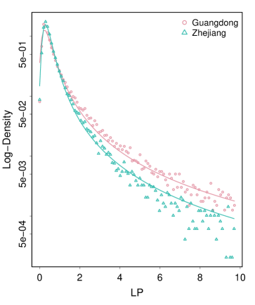
(a) $LP$

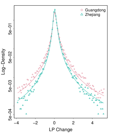
(b) $\Delta LP$

Figure 6: Density of $LP$ and $\Delta LP$ for regions Guangdong and Zhejiang in 2007

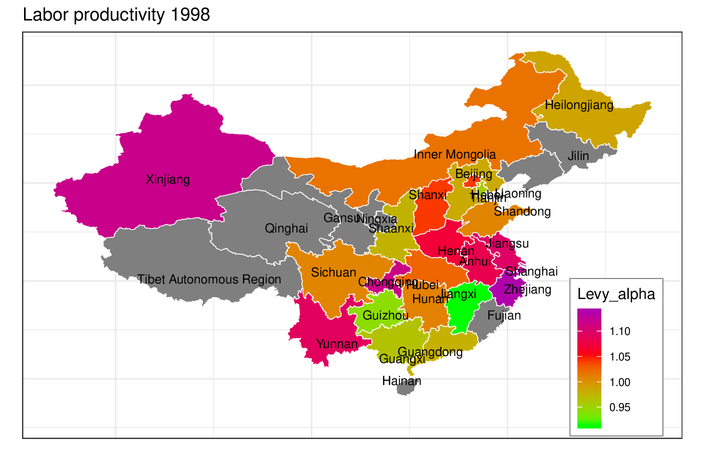
(a) 1998

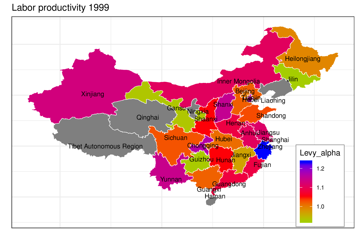
(b) 1999

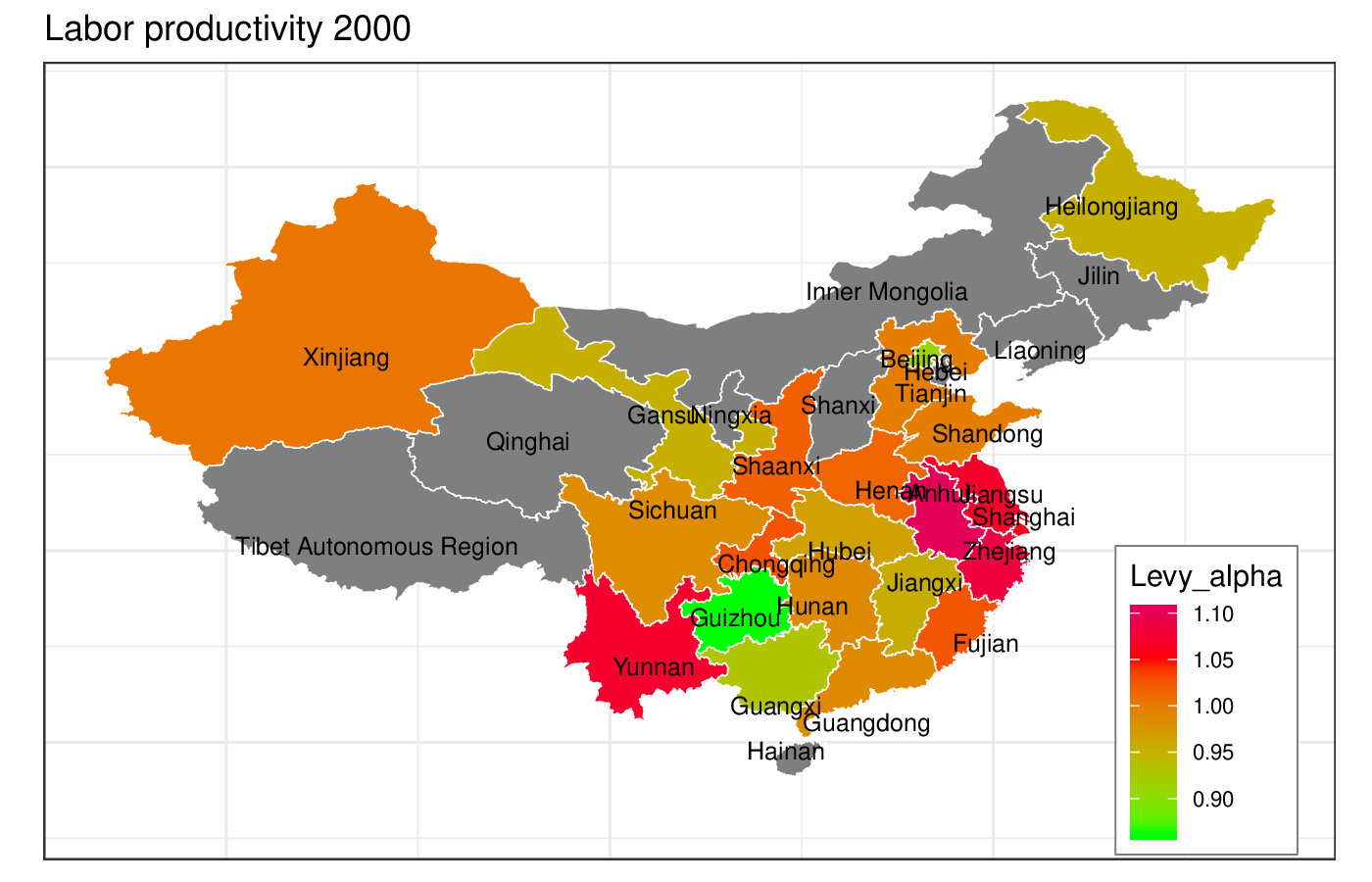
(c) 2000

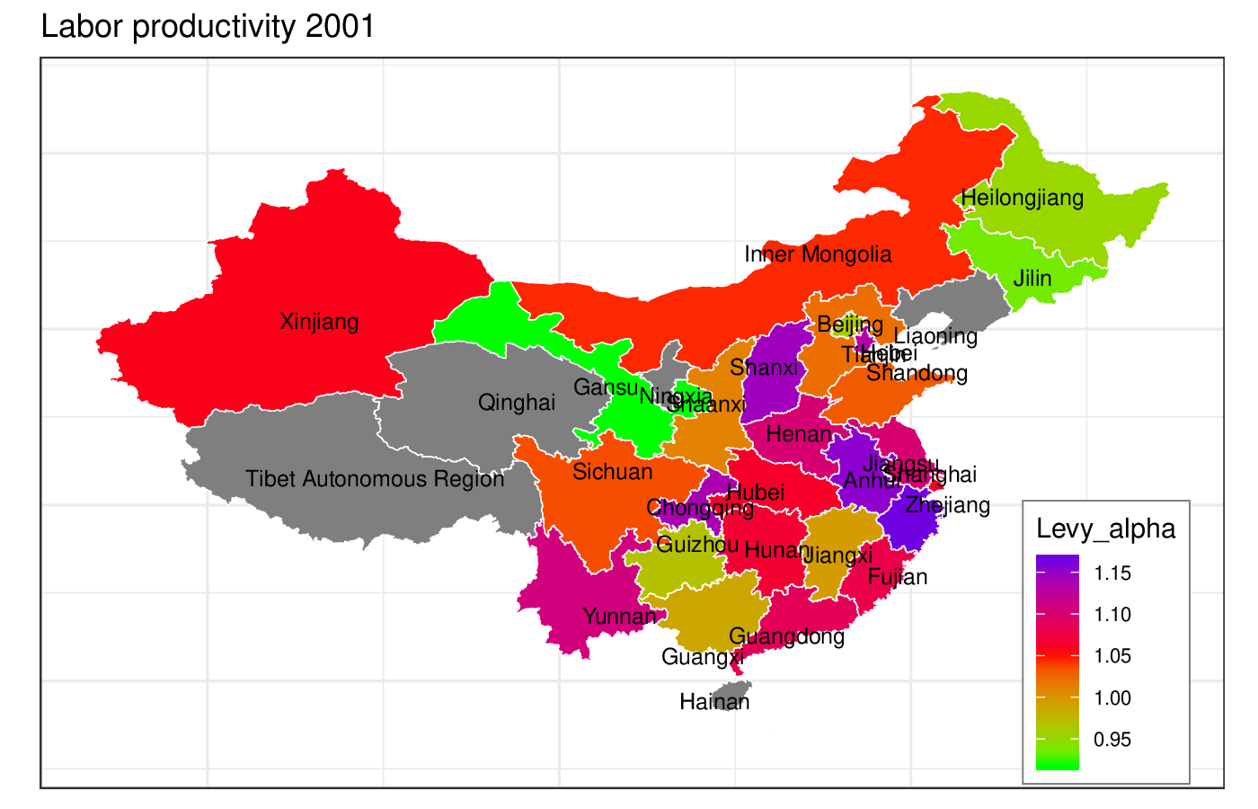
(d) 2001

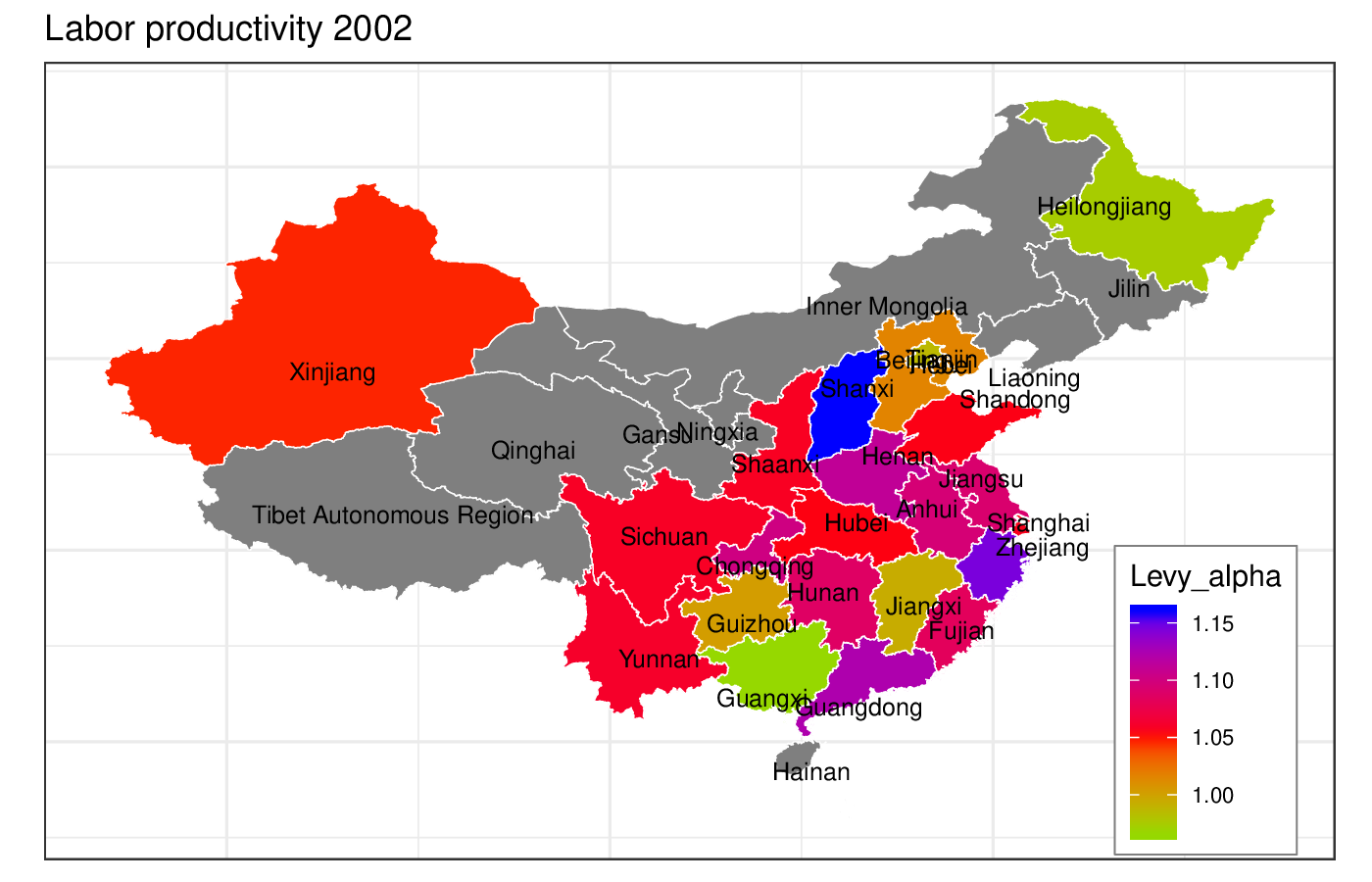
(e) 2002

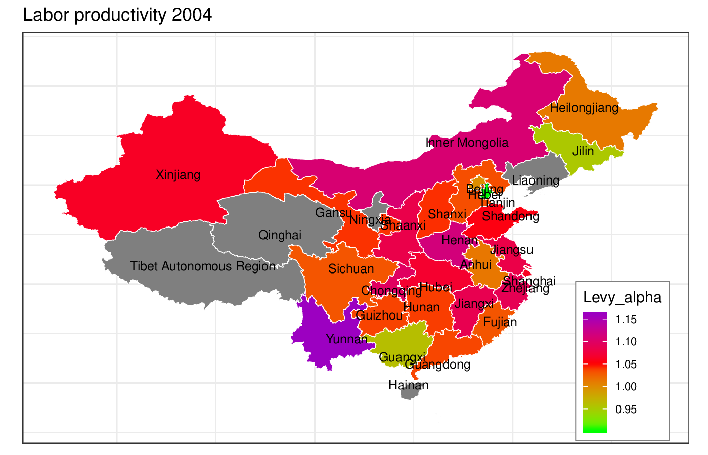
(f) 2004

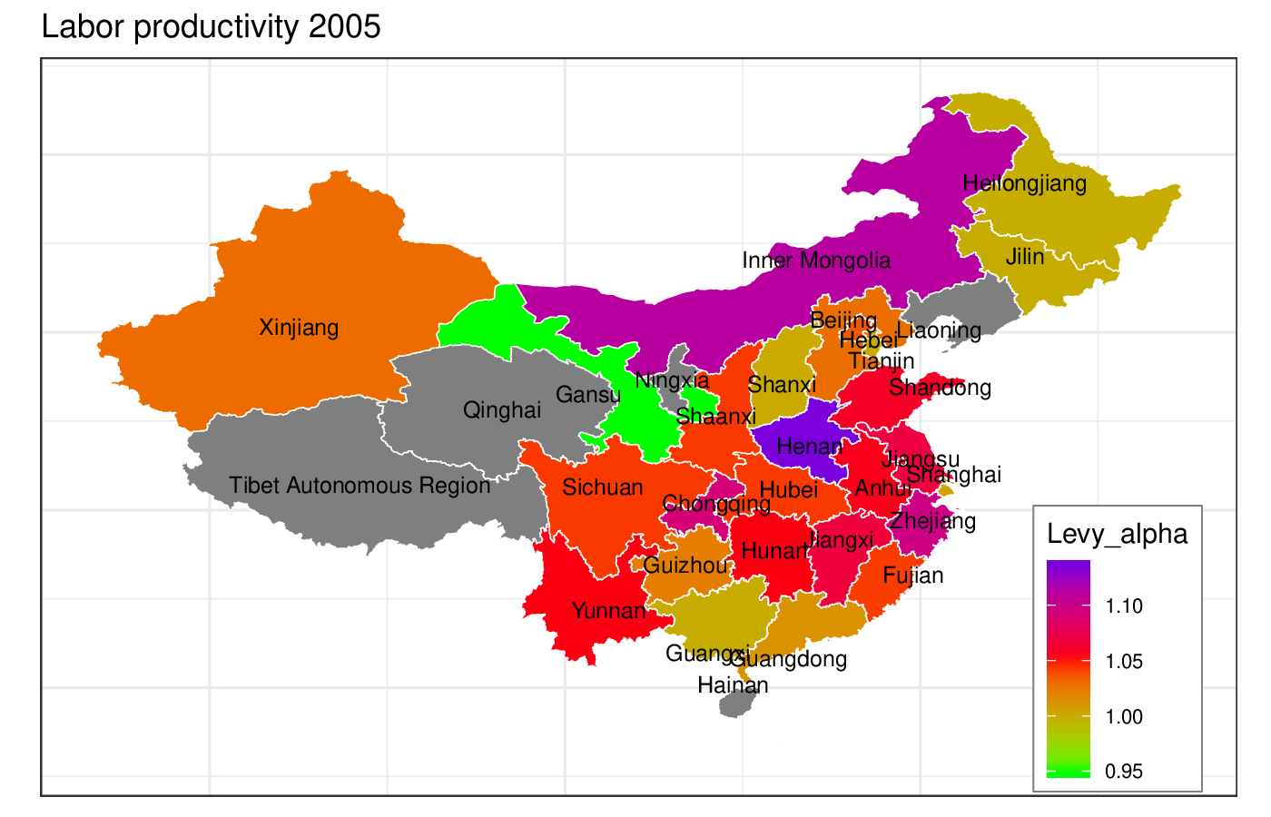
(g) 2005

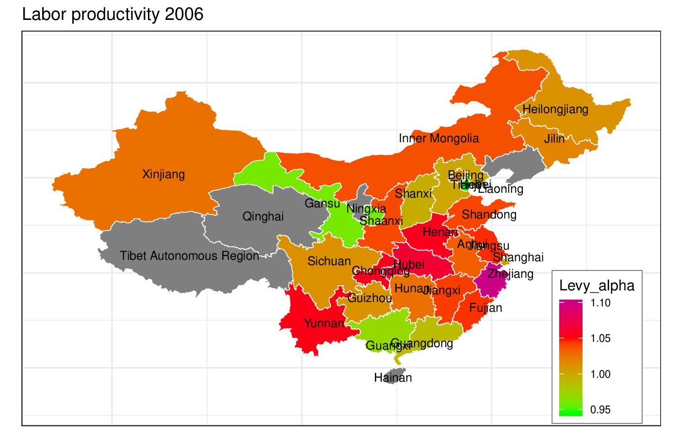
(h) 2006

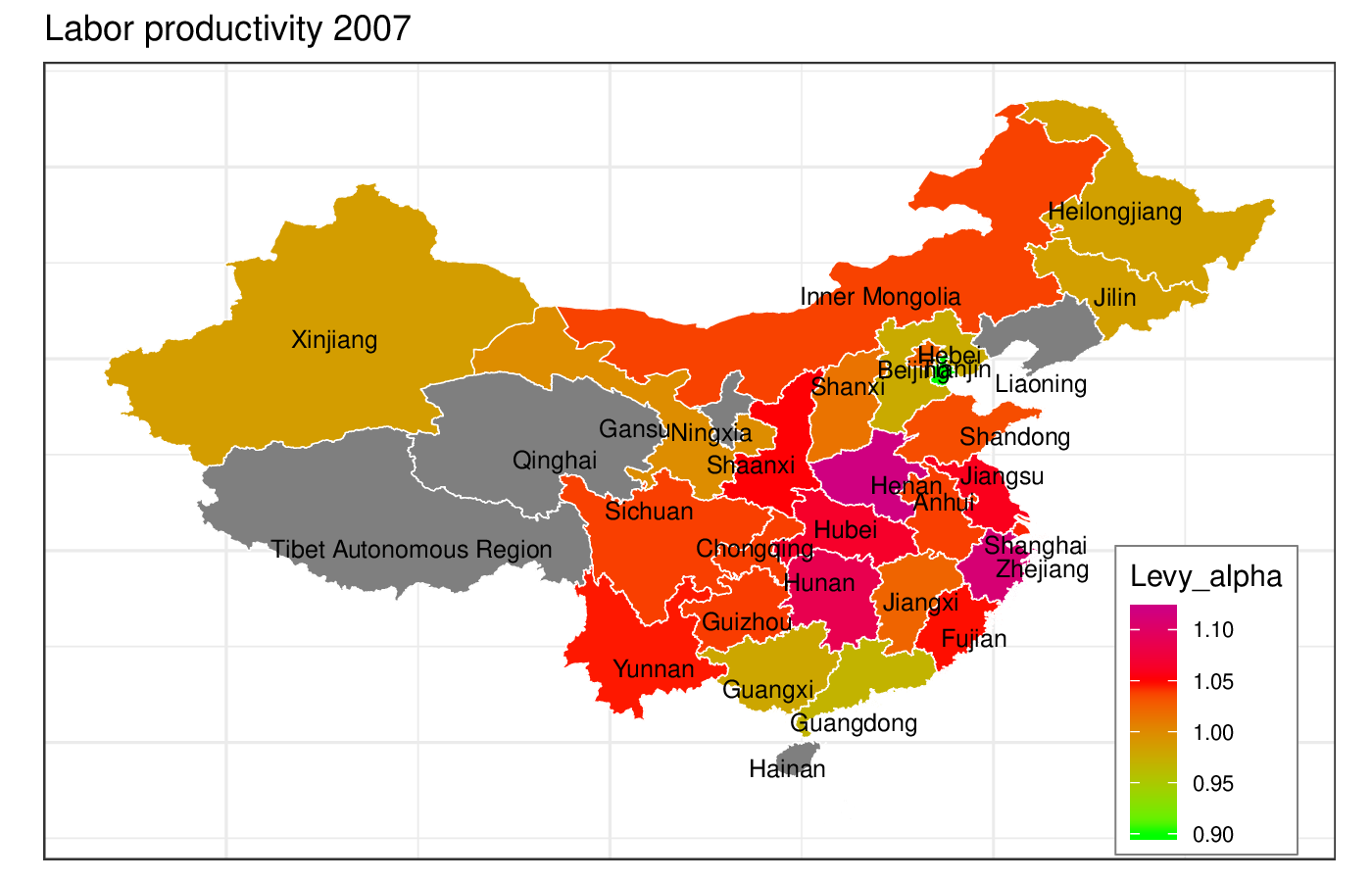
(i) 2007

Figure 7: Levy $\alpha$ parameter fits for $LP$ (labor productivity) by Region

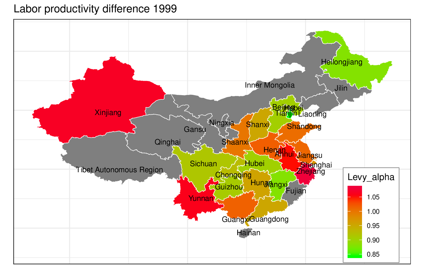
(a) 1999

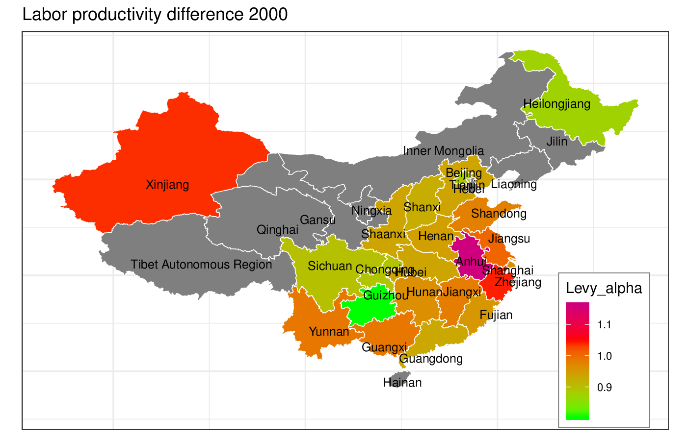
(b) 2000

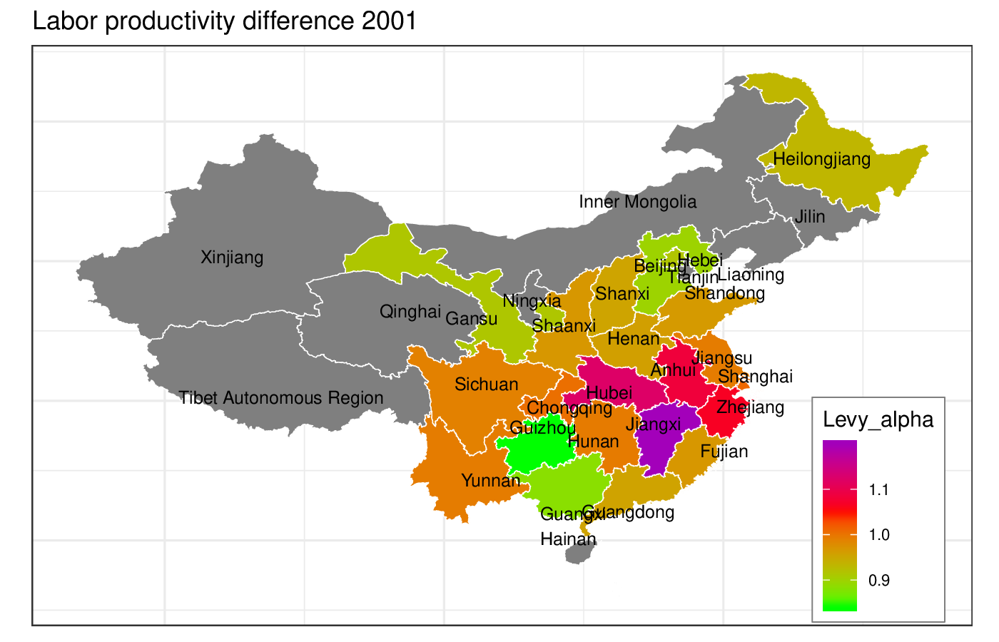
(c) 2001

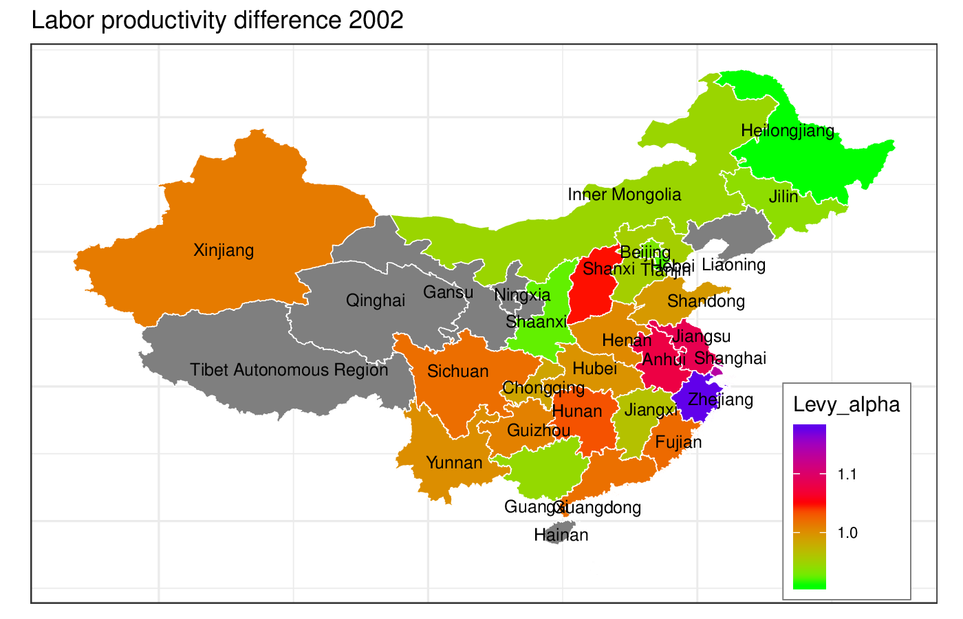
(d) 2002

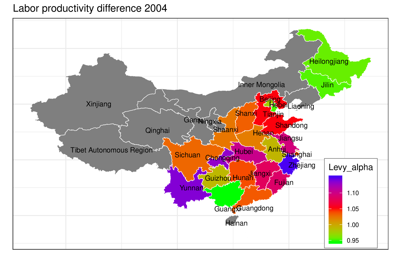
(e) 2004

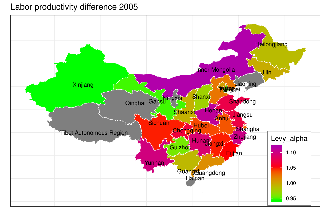
(f) 2005

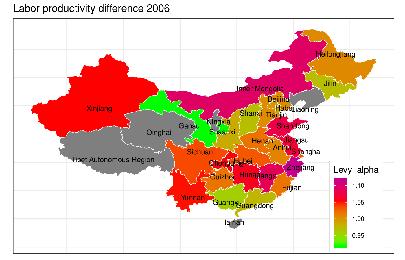
(g) 2006

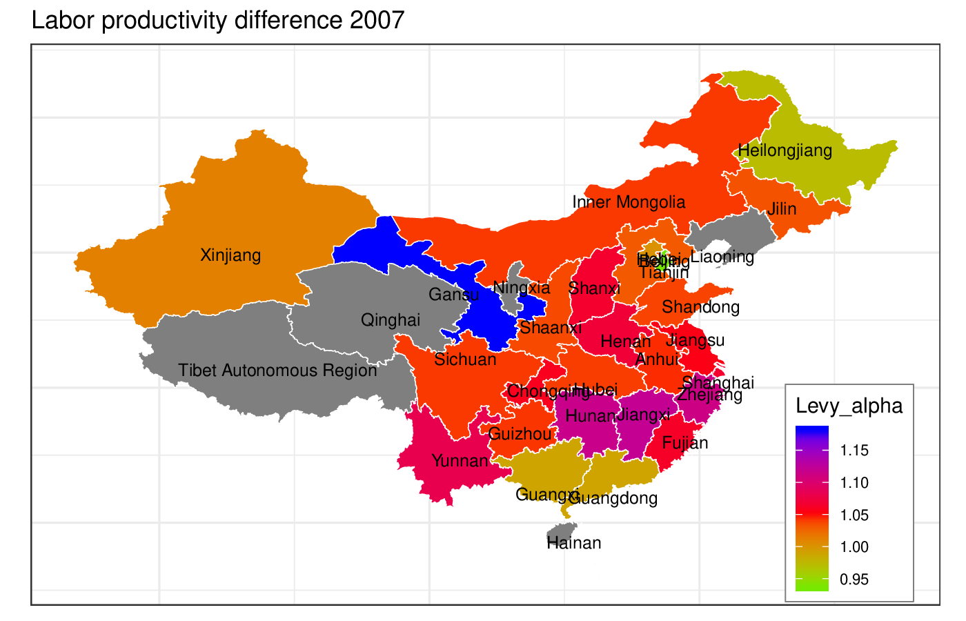
(h) 2007

Figure 8: Levy $\alpha$ parameter fits for $\Delta LP$ (labor productivity change) by Region

5.3 Regional variation

While we only have data for one country, the P.R. China, we can investigate regional variation by considering subsamples of the data set for the 31 Chinese provinces and autonomous regions. In cross-country studies, where the cases are not subject to the same policy decision and idiosyncratic influences, any systematic differences should be more pronounced.

Two of the most dynamic and economically strongest regions of the PR China are Guangdong and Zhejiang. While Zhejiang is one of the most active regions supporting private economic sectors, and has benefited from the early economic boom in Yangtze River Delta, Guangdong is in South China, north of Hong Kong, and driven significantly by the opening-up endeavors. Both are coastal provinces and have the potential to develop the same industries. Yet, the regional distributions of $LP$ and $\Delta LP$ differ sharply and persistently. Guangdong maintains one of the lowest tail indices among all provinces, i.e. a very high probability weight in the tails ($\alpha_{\Delta LP}=0.93$ to $\alpha_{\Delta LP}=1.03$). Zhejiang is at the other end of the provincial dispersion, with a moderately high tail index between $\alpha_{\Delta LP}=1.05$ and $\alpha_{\Delta LP}=1.18$. Figure 6 shows the density of labor productivity $LP$ and labor productivity change $\Delta LP$ in both regions.

Figures 7 and 8 show the development of the tail index parameter $\alpha$ of the Lévy alpha-stable fit of labor productivity $LP$ and labor productivity change $\Delta LP$ at the region level. Indeed it can be seen that Guangdong and neighboring regions (Guangxi, Jiangxi) and Zhejiang and its neighbors (Shanghai, Anhui) persistently find themselves at opposing ends of the variation. The Guangdong area tends to have longer tails (lower exponents) than the Shanghai/Zhejiang area.

Other regions with longer tails include the Northeast (Heilongjiang), the Beijing region, Inner Mongolia and, in the earlier years of the period of study, the central region. As pointed out in Heinrich and Dai (2016), this subtle change over time may reflect the transition of various regions to a standard market economy system that occurred at different time periods (see details in Heinrich and Dai (2016)). Some regions, such as Inner Mongolia, likely stand out because of regional specificities; in Inner Mongolia a domination of the mining sector with rather large firms and certain volatility of empirical labor productivity depending on world market prices for metals etc. Some regions with a smaller population of firms (Xinjiang, Guangsu) are more volatile with less confidence being warranted for these fits.

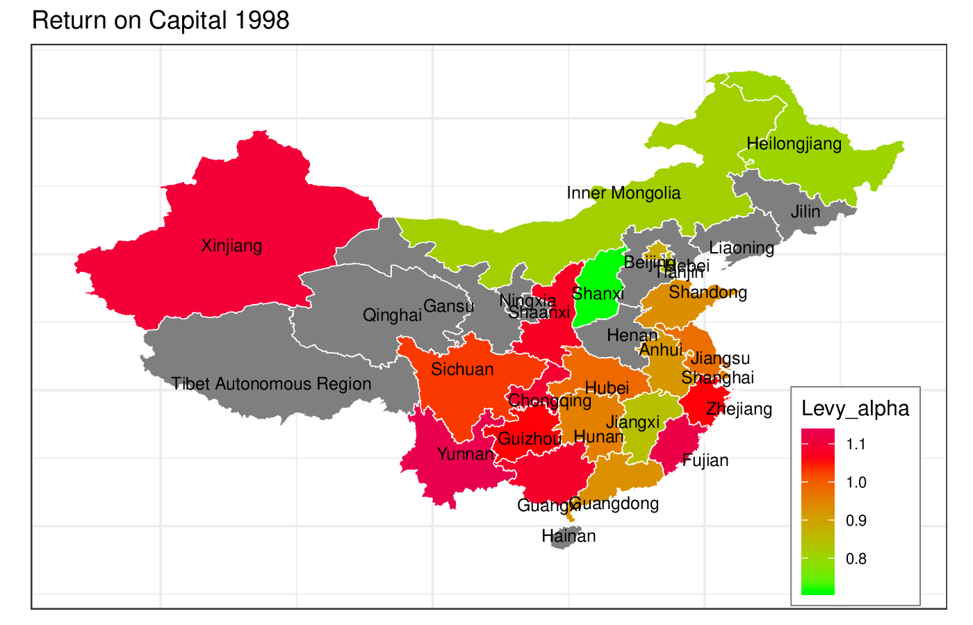
(a) 1998

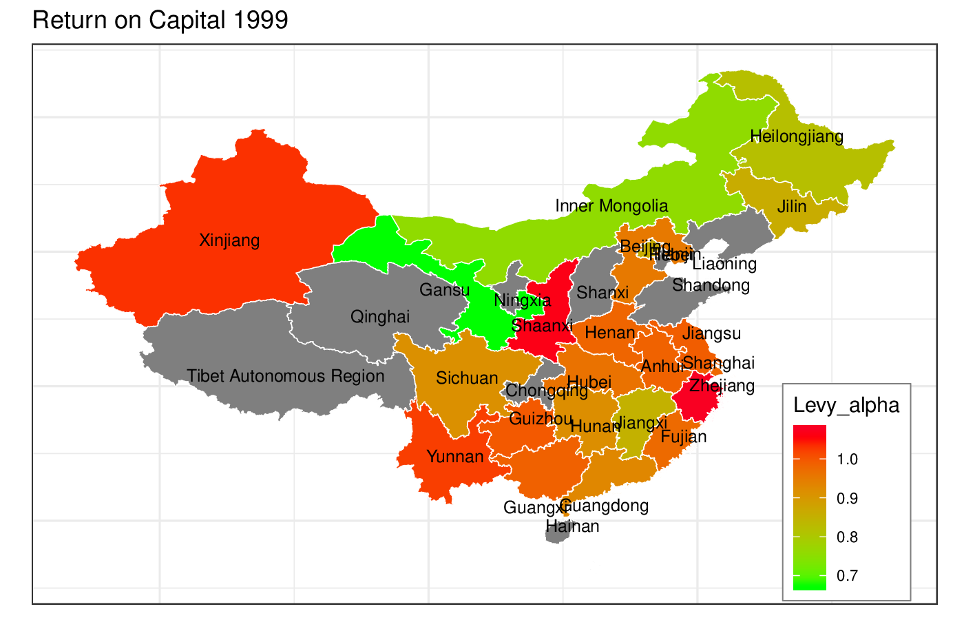
(b) 1999

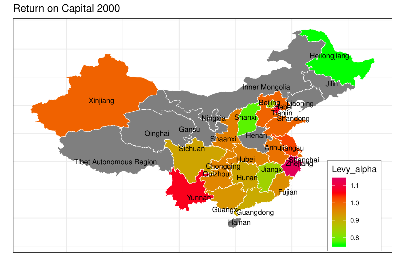
(c) 2000

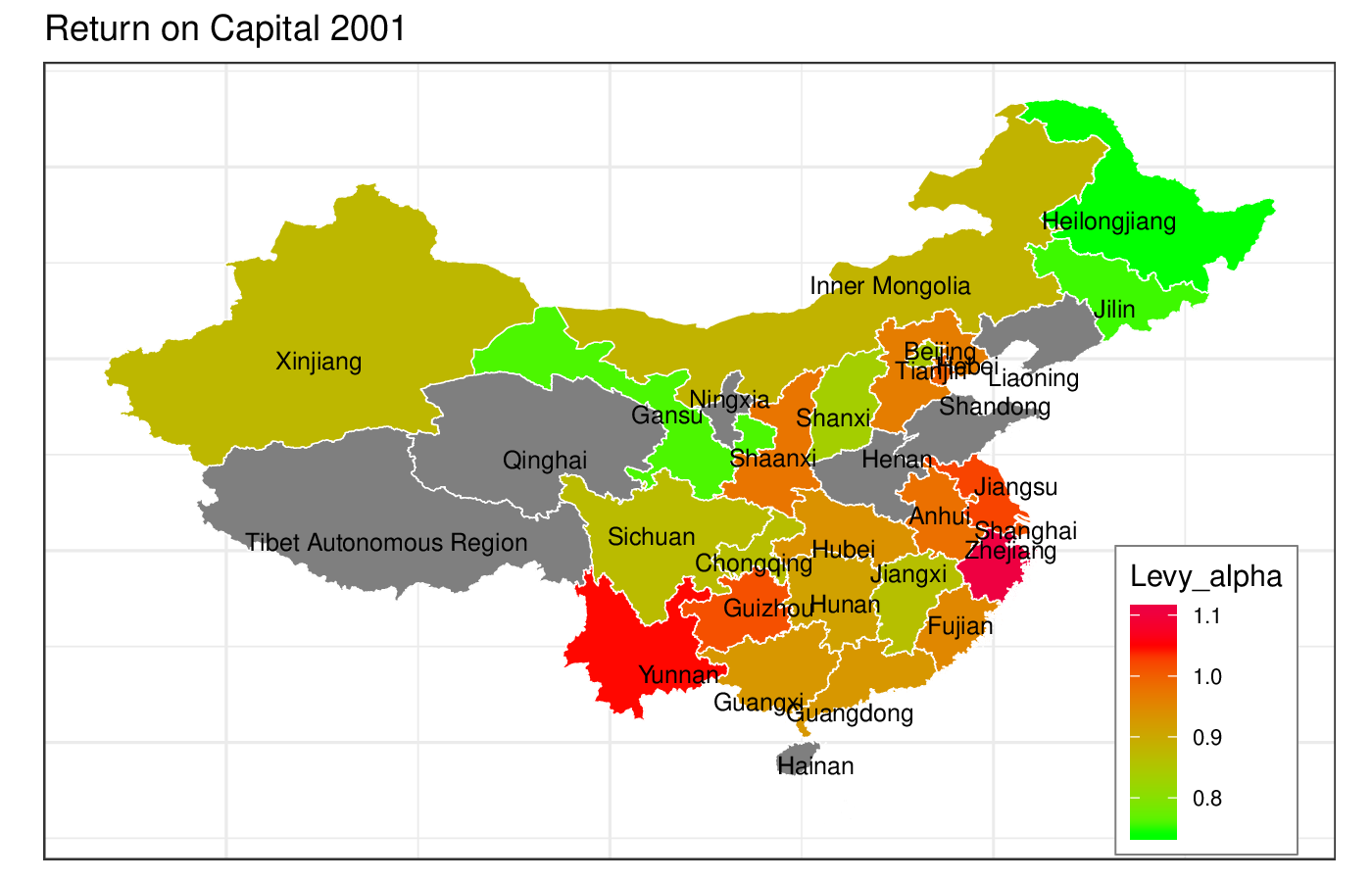
(d) 2001

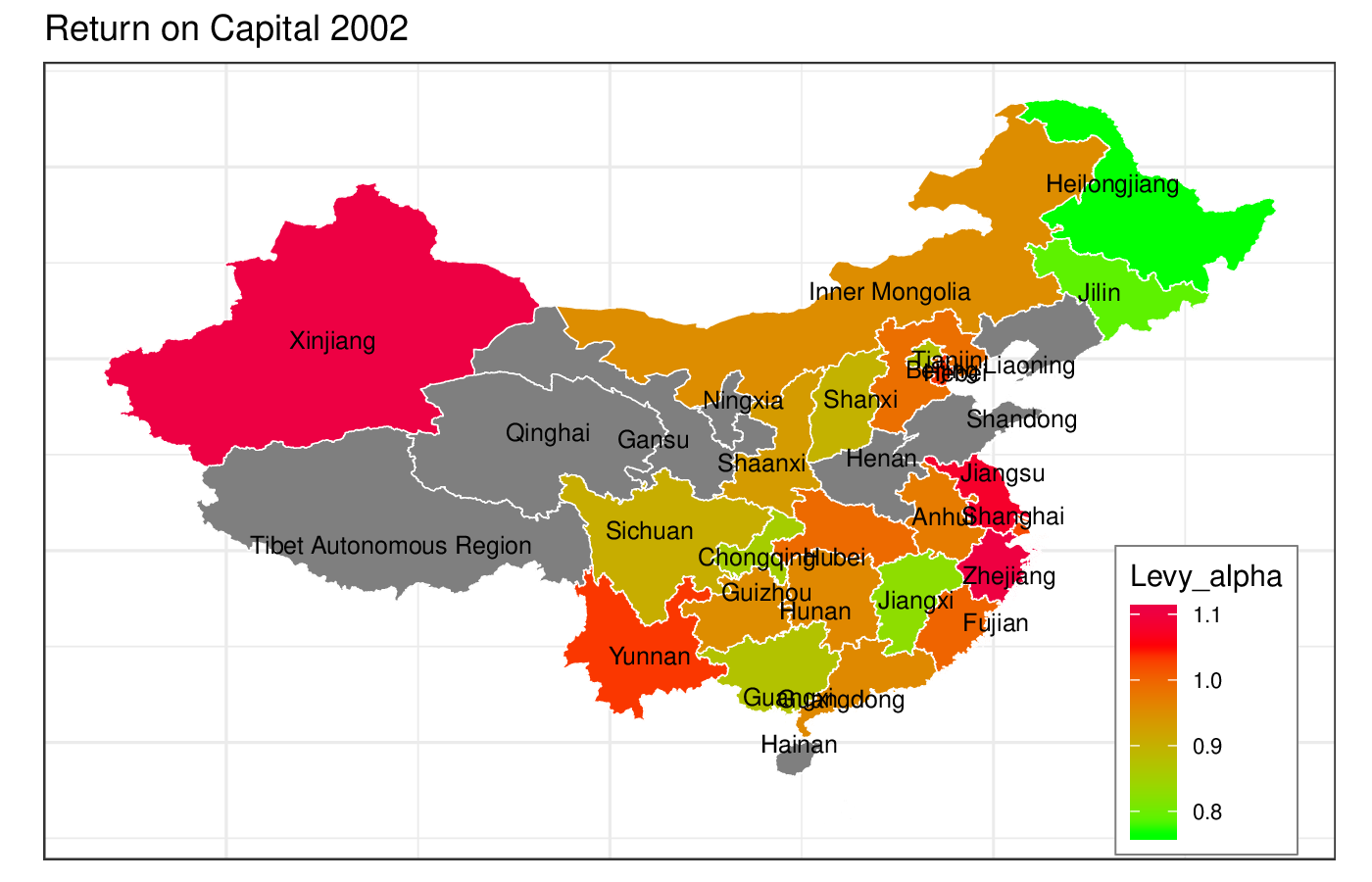
(e) 2002

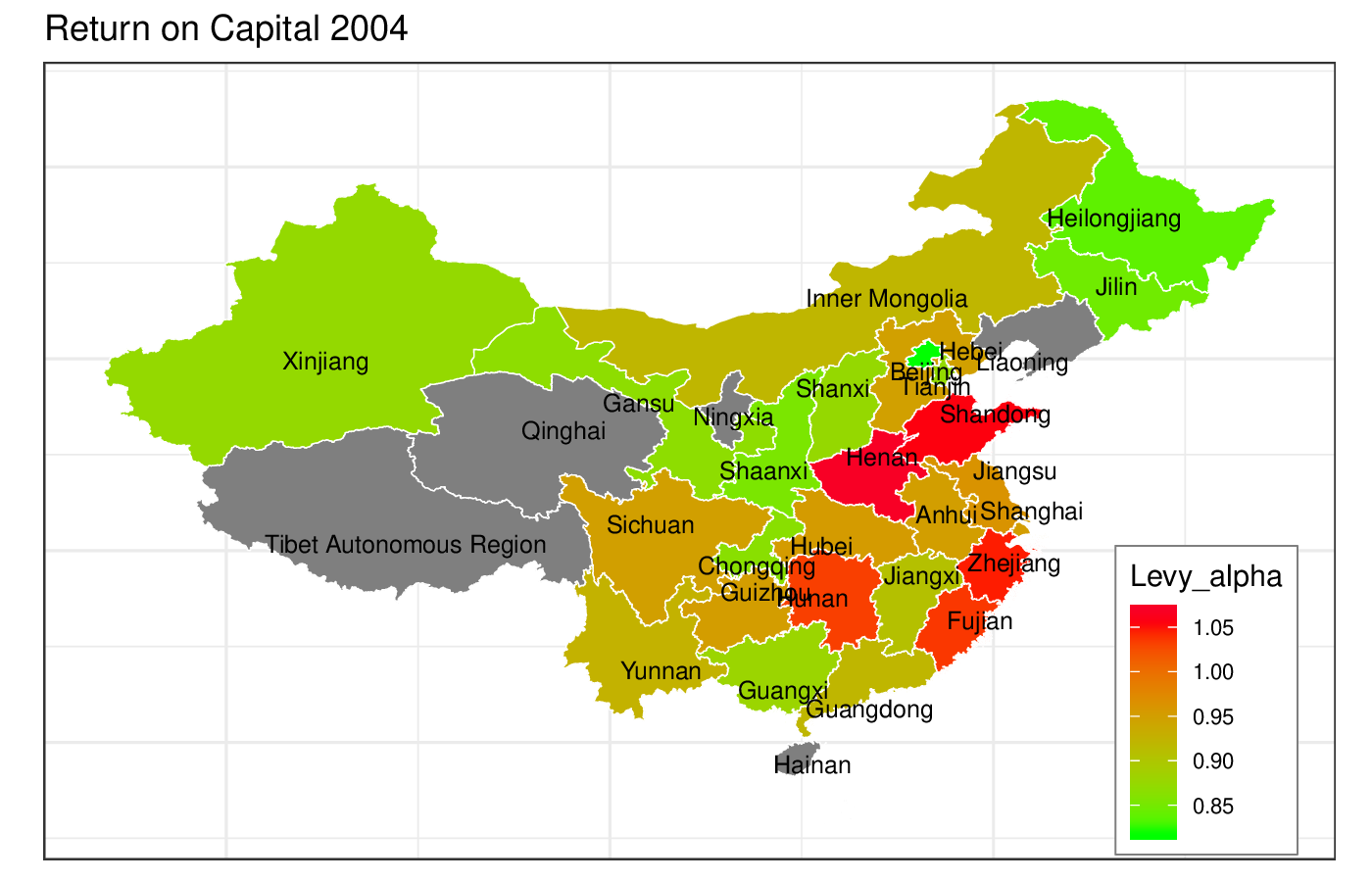
(f) 2004

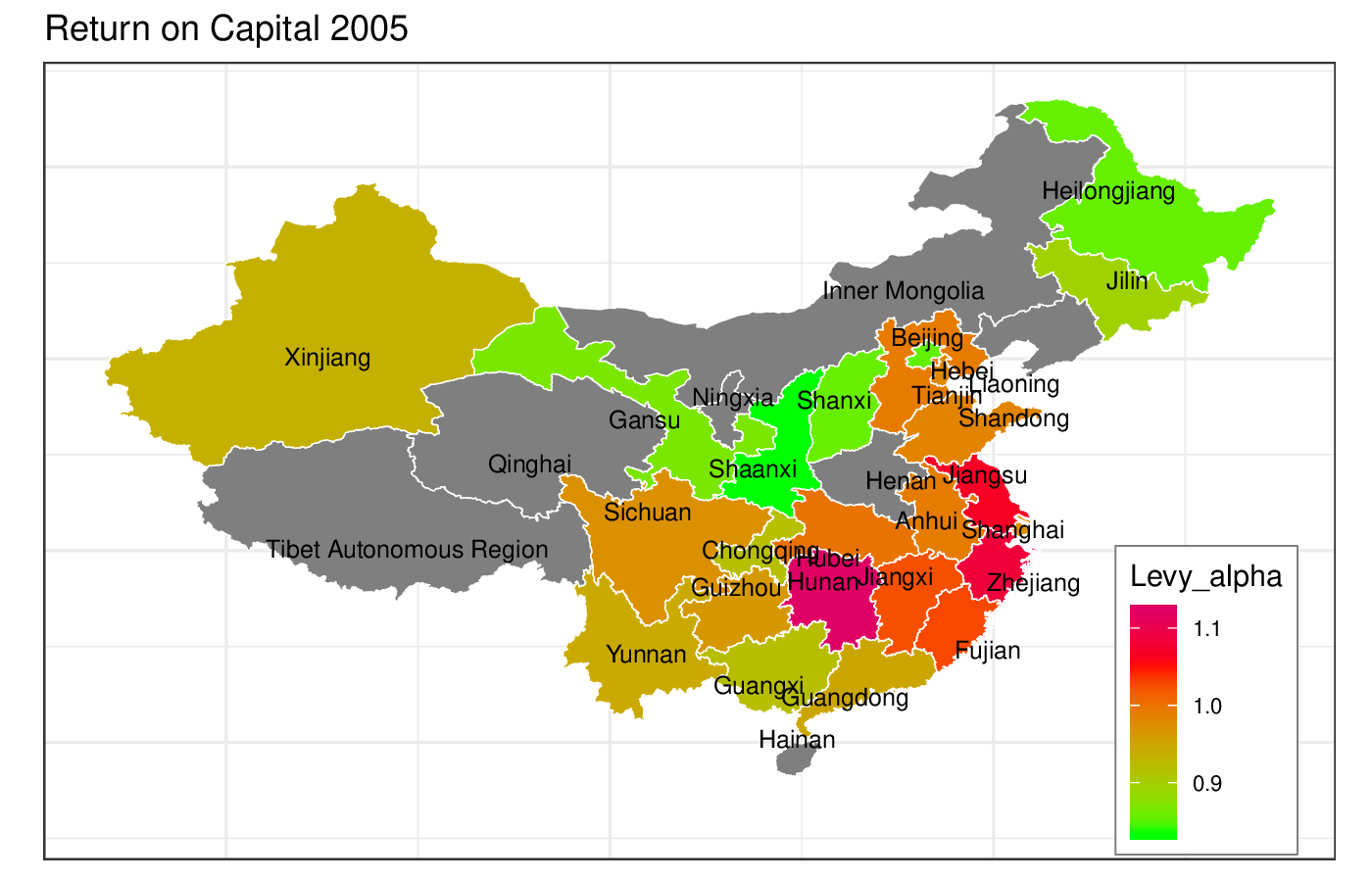
(g) 2005

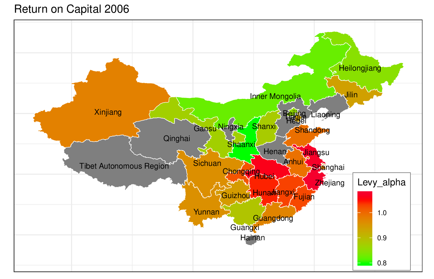
(h) 2006

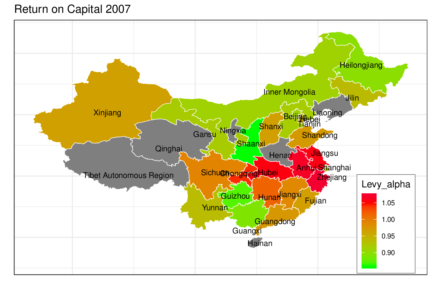
(i) 2007

Figure 21: Levy $\alpha$ parameter fits for $ROC$ (profitability) by Region

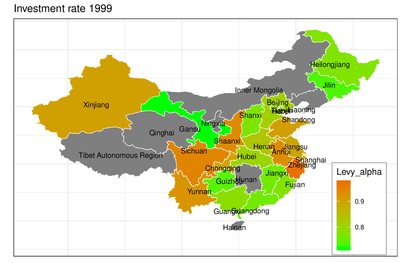
(a) 1999

(b) 2000

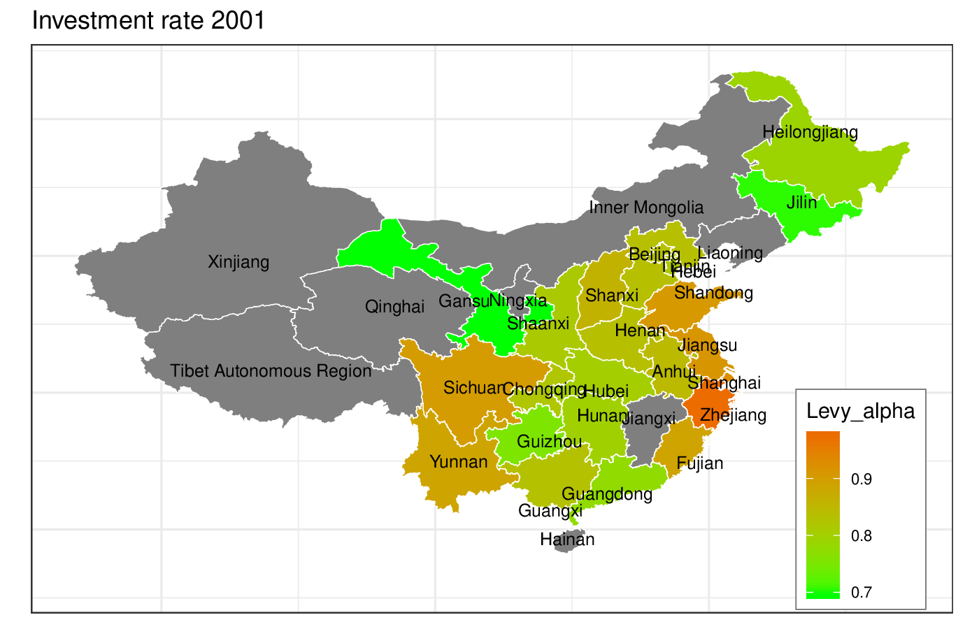
(c) 2001

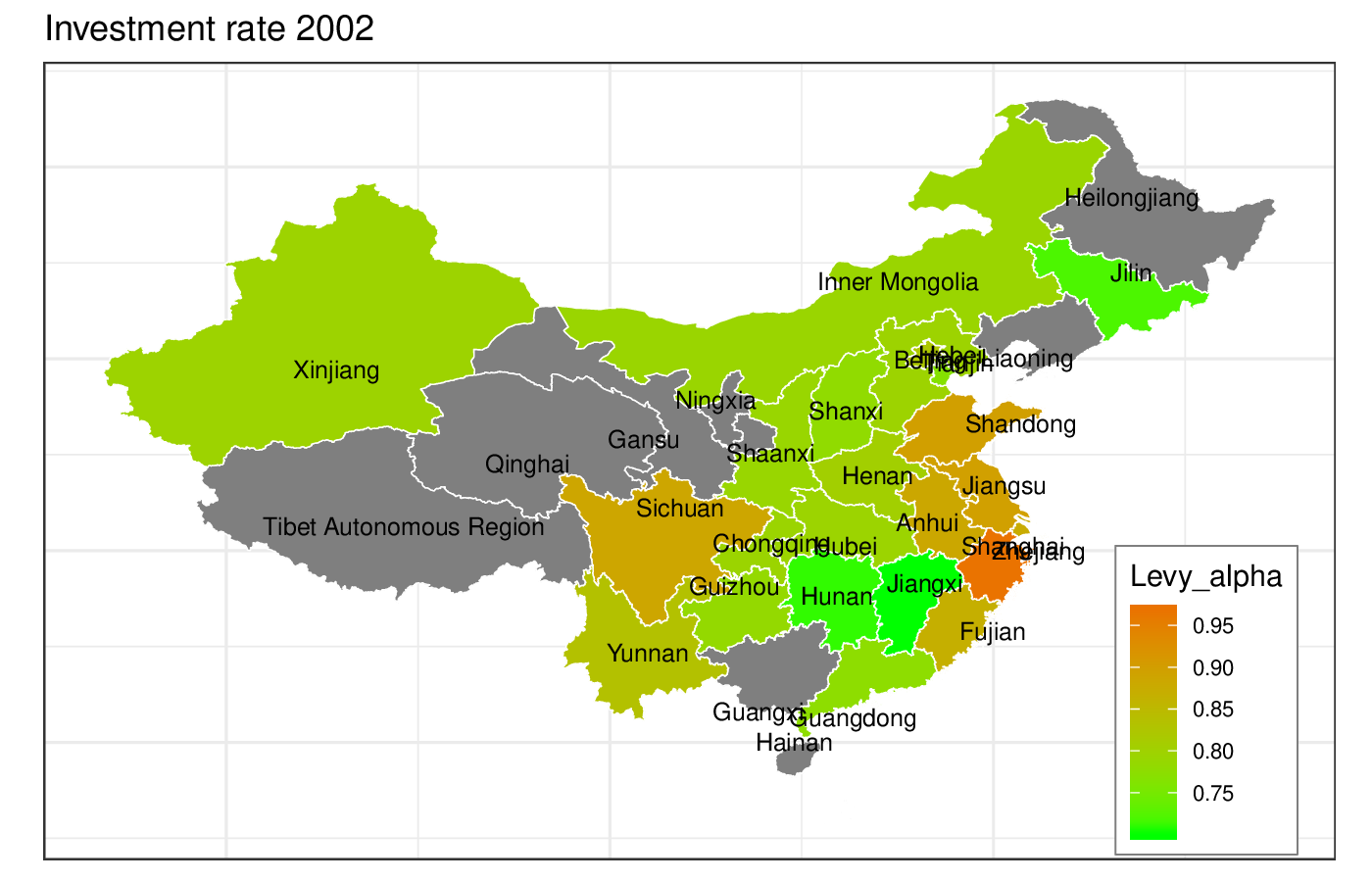
(d) 2002

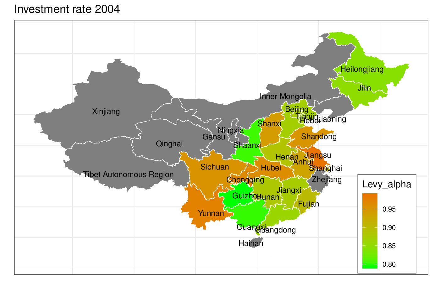
(e) 2004

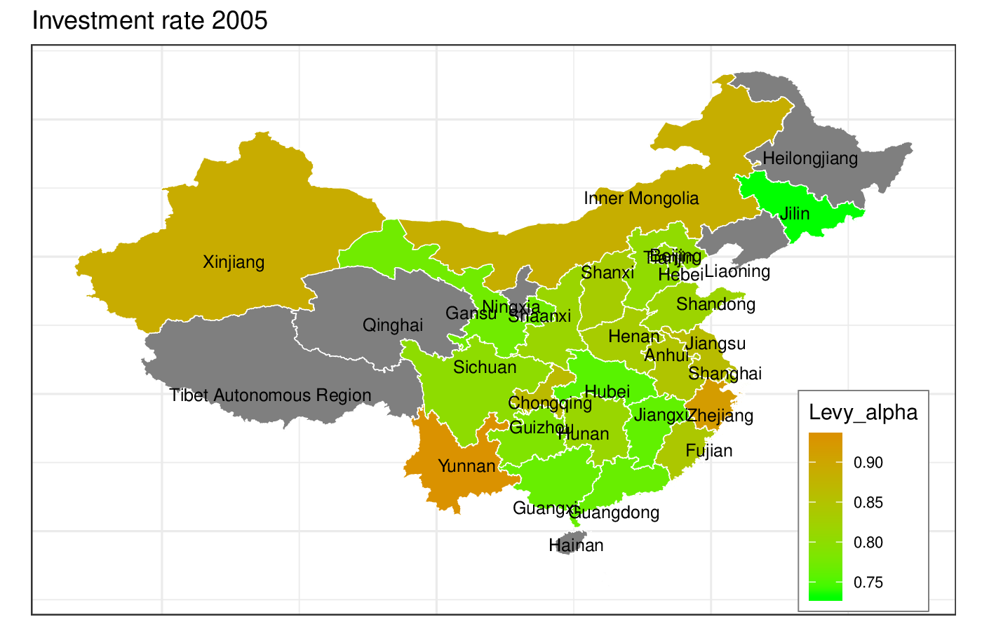
(f) 2005

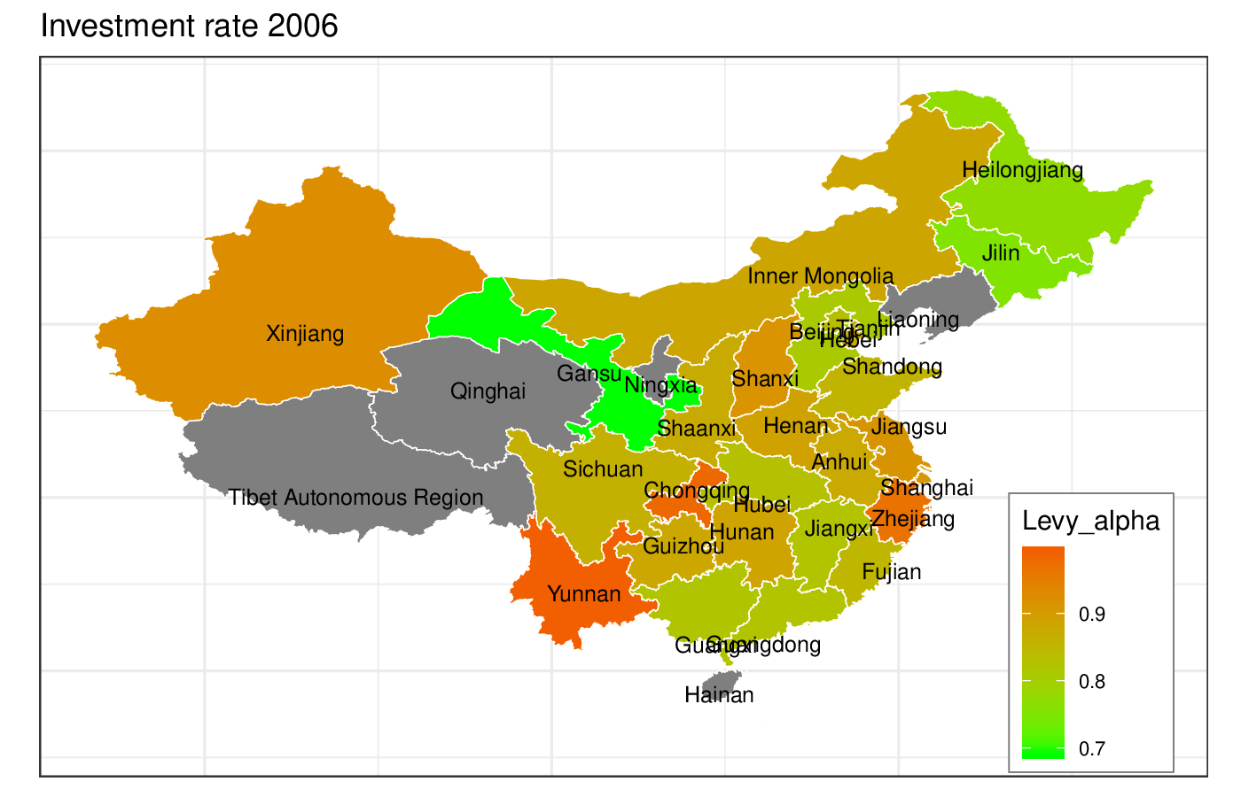
(g) 2006

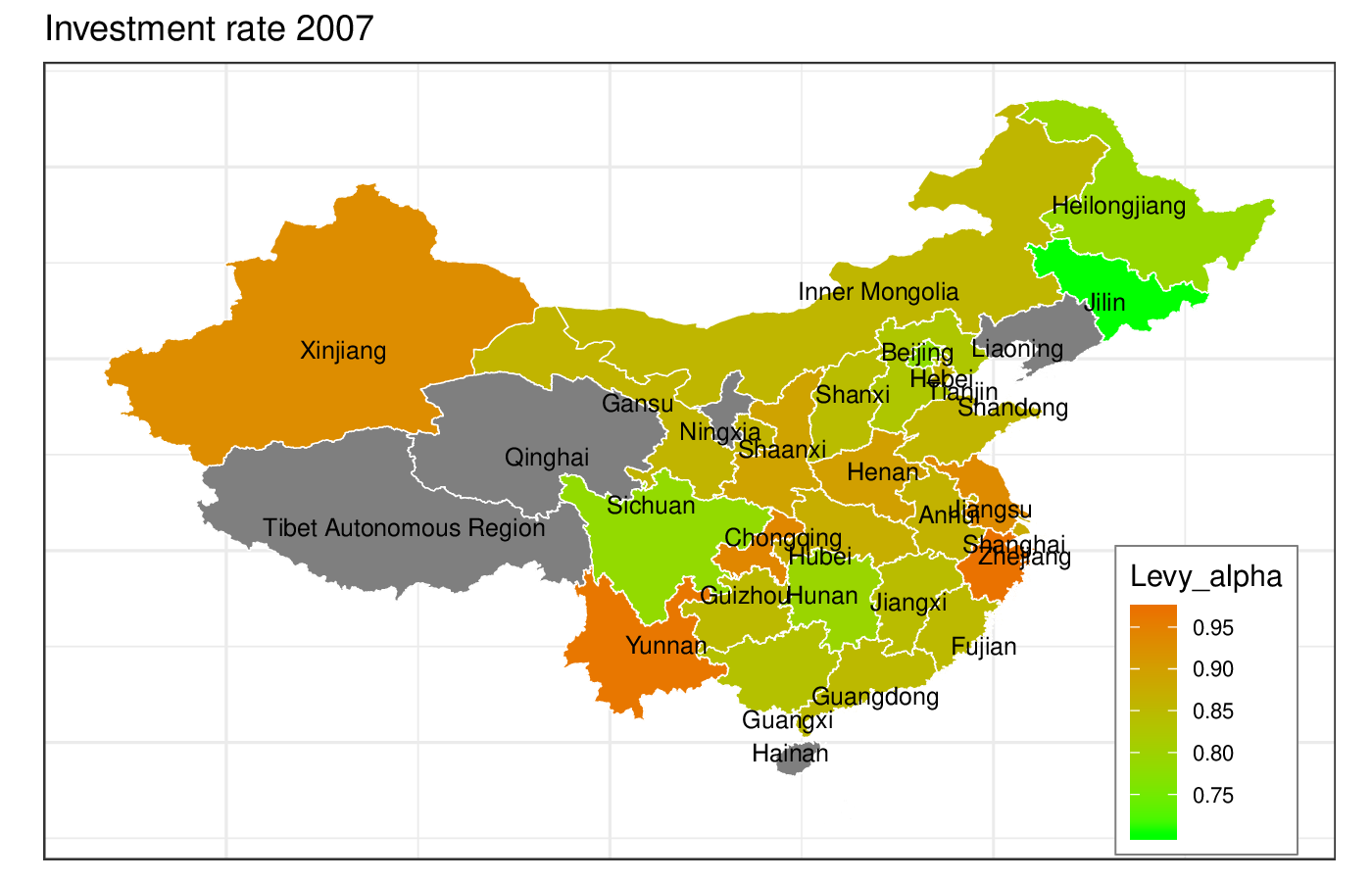
(h) 2007

Figure 22: Levy $\alpha$ parameter fits for $IR$ (investment return) by Region

So far, we have shown that there are strong and persistent differences in the characteristics of the productivity distributions among the regions of China. This indicates that this would very likely also hold between countries. Beyond that, we can show in the Chinese case that micro-level variables are strongly interconnected: For instance, there is a cluster of regions with a shorter tail (higher tail index $\alpha$) around Shanghai and Zhejiang in both $LP$ (Figure 7) and $\Delta LP$ (Figure 8). This regional pattern is also present in the figures for profitability and the investment rate shown in the Appendix D (Figures 21 and 22). Indeed, it can be shown that at the regional level, the distributions of the key firm-level variables are interconnected. The correlations of parameters fitted for the labor productivity change ($\Delta LP$) distribution and investment rate ($IR$) distribution are shown in Figure 9; those of the parameters for ($\Delta LP$) and the profitability ($ROC$) are plotted in Figure 10. For each pair of distributions, the same parameters are highly correlated. I.e. a high tail index $\alpha$ for the labor productivity change distribution is associated with a high tail index for the distributions of profitability and investment rate. The same is true for the skew ($\beta$) and the scale ($\gamma$) of all distributions and the location of the modal value ($\delta$) of $\Delta LP$ and $ROC$ distributions.

These systematic regional differences evident in concert in a number of variables in the Chinese case indicate that such patterns should also be expected in cross-country comparisons. The following section will furthermore investigate relations between productivity distributions and various other macro- and micro-level variables using a Bayesian multi-level regression approach.

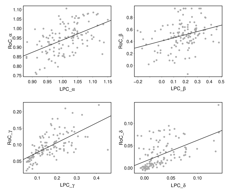
Figure 9: Scatter plot of Lévy parameters of Returns on Capital ($ROC$) and Labor Productivity Change ($\Delta LP$). All four parameters tend to be positively correlated.

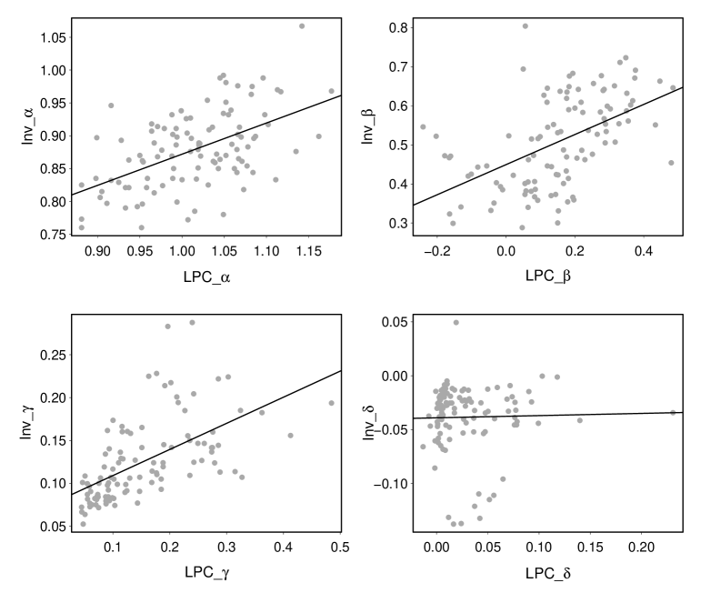
Figure 10: Scatter plot of Lévy parameters of Investment Rate ($IR$) and Labor Productivity Change ($\Delta LP$). $\alpha,\beta,\gamma$ tend to be positively correlated, while $\delta$ has no relationship.

5.4 Relation of productivity distributions and their parameters to other economic measures

To understand how Lévy parameters of each variable are associated with the geographical predictors (in this case, Chinese regions), we run a simple mixed linear regression model. We use a Bayesian multi-level approach to properly account for group-level similarities and differences through a partial pooling. The likelihood function is written as follows:

$$\operatorname{Parameter_{i}} \sim \operatorname{Normal}(\mu_{i},\sigma)$$

$$\mu_{i} = \alpha+\alpha_{{}_{j[i]}}+\alpha_{{}_{t[i]}}+\beta_{1}\operatorname{GDP\_r}+\beta_{2}\operatorname{Firm\_Age}+\beta_{3}\operatorname{Emp}+\beta_{4}\operatorname{Cap\_Intensity}$$ (5)

where the subscript $t[i]$ and $j[i]$ indicate the year and province index which will be used as the main group effect variable. See Appendix B for a detailed discussion on prior specification. We assume that the outcome variable $\operatorname{Parameter_{i}}$ is distributed according to the Gaussian likelihood function around a mean $\mu_{i}$ and the standard deviation $\sigma$. The independent variables (predictors) include GDP growth (GDP_r), firm age, employment (Emp), as well as capital intensity ($\operatorname{Cap\_Intensity}$) at the regional level. The firm-level variables among these (not the GDP growth) are computed using the regional averages in the data set. The intercept has two varying components by year and province along with the overall intercept.

• $\alpha$: The overall intercept. The expected value of $\operatorname{Parameter_{i}}$ when all other explanatory variables are zero.

• $\alpha_{{}_{t[i]}}$: The varying intercept effect coming from the year index. The deviation in the intercept for year $t$ from the overall intercept $\alpha$.

• $\alpha_{{}_{j[i]}}$: The varying intercept effect coming from the province index. The deviation in the intercept for province $j$ from the overall intercept $\alpha$.

• $\beta_{1}$: The coefficient of GDP Growth. The expected change in $\operatorname{GDP\_Growth}$ across all $t$ and $j$.

• $\beta_{2}$: The coefficient of Firm Age. The expected change in $\operatorname{Firm\_Age}$ across all $t$ and $j$.

• $\beta_{3}$: The coefficient of Employment. The expected change in $\operatorname{Employment}$ across all $t$ and $j$.

• $\beta_{4}$: The coefficient of Capital Intensity. The expected change in $\operatorname{Capital\_Intensity}$ across all $t$ and $j$.

We use the Hamiltonian Monte Carlo (HMC) to obtain a sequence of random samples from a posterior probability distribution. We use the Bayesian programming language Stan and the R-package brms that operationalize the HMC algorithm to efficiently compute posterior distributions (Stan Development Team, 2015; Bürkner, 2017). For a more detailed discussion on HMC and Stan, see (Gelman et al., 2014; Carpenter et al., 2017).

Table  4 summarizes the estimation results for each variable and parameter. We only report the mean and standard deviation (in parenthesis) of the posterior distribution of each parameter. A full summary table can be found in the Appendix 22.

Variable	Parameters	Intercept	GDP Growth	Firm Age	Employment	Capital Intensity
LP Change	$\alpha$	0.9841 (0.0462)	0.0083 (0.0027)	-0.0012 (0.0006)	-0.0001 (0.0001)	-0.0001 (0.0001)
	$\beta$	-0.0564 (0.1025)	0.0256 (0.0065)	-0.0035 (0.0014)	0 (0.0001)	-0.0001 (0.0002)
	$\gamma$	0.0555 (0.0466)	0.0094 (0.0026)	0 (0.0005)	-0.0002 (0.0001)	0.0004 (0.0001)
	$\delta$	-0.0105 (0.024)	0.0054 (0.0014)	-0.0001 (0.0003)	-0.0001 (0)	0 (0)
LP	$\alpha$	1.0823 (0.0509)	0.0007 (0.0031)	-0.0001 (0.0002)	-0.0001 (0.0001)	-0.0001 (0.0001)
	$\gamma$	0.2304 (0.063)	0.0054 (0.0032)	0 (0.0002)	-0.0005 (0.0001)	0.0004 (0.0001)
	$\delta$	0.2574 (0.0681)	0.009 (0.0035)	0 (0.0002)	-0.0005 (0.0001)	0.0003 (0.0001)
RoC	$\alpha$	1.1235 (0.0564)	-0.0033 (0.0033)	-0.0008 (0.0002)	-0.0003 (0.0001)	-0.0001 (0.0001)
	$\beta$	0.167 (0.1337)	0.0333 (0.0081)	0 (0.0004)	-0.0003 (0.0002)	-0.0001 (0.0002)
	$\gamma$	0.0713 (0.0208)	0.0034 (0.0012)	-0.0001 (0.0001)	0 (0)	-0.0001 (0)
	$\delta$	0.0341 (0.0181)	0.0018 (0.0011)	0 (0.0001)	-0.0001 (0)	-0.0001 (0)
Inv Rate	$\alpha$	0.7954 (0.0486)	0.0004 (0.0025)	-0.0014 (0.0008)	0.0002 (0.0001)	0.0002 (0.0001)
	$\beta$	0.4201 (0.0955)	0.0047 (0.0044)	0.0005 (0.0015)	-0.0001 (0.0001)	0.0001 (0.0002)
	$\gamma$	0.122 (0.0286)	0.0028 (0.0016)	-0.0007 (0.0005)	0 (0)	0 (0.0001)
	$\delta$	-0.0687 (0.0191)	-0.0001 (0.0009)	-0.0001 (0.0003)	0.0001 (0)	0 (0)

Table 4: Summary statistics of a mixed linear regression model of Lévy parameters with four predictors: GDP Growth, Firm Age, Employment, and Capital Intensity.

For each variable, we show the regression results for Lévy parameters. Note that we do not report on the regression of $\beta$ in the labor productivity variable since it is always very close to 1 (maximal skewness) and doesn’t have much variation.

GDP Growth

:

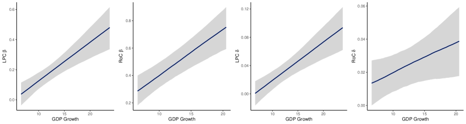
Figure 11: Marginal effects of GDP Growth on $\beta$ and $\delta$ of labor productivity change ($\Delta LP$) and profitability ($ROC$). The blue line is the mean estimate and the grey shade area is the 90% uncertainty interval.

A higher regional economic growth tends to be associated with a higher $\beta,\gamma$, and $\delta$ in $\Delta LP$ and profitability. The GDP coefficients in labor productivity and investment rate tend to be rather noisy except for $\gamma$. $\alpha$ parameter is only informative in the $\Delta LP$ case: the higher the provincial GDP growth the higher $\alpha$ and thus the thinner the tails. $\alpha$ in other variables has neither enough variation nor a clear pattern in relation to regional GDP growth. Figure 11 shows the marginal effects of GDP Growth on key parameters. From this, we can infer that the economic growth in China is characterized by four distinctive patterns. As the economy grows in China, 1) firms become more technologically dynamic and more profitable (a high $\delta$ in $\Delta LP$ and profitability), 2) the economy has an increasing number of highly innovative and profitable firms (a high $\beta$ in $\Delta LP$ and profitability), 3) firms become more diverse in their performance (a high $\gamma$ in $\Delta LP$, $LP$, profitability and investment rate), and 4) the technological competition among firms gets more fierce over time (a high $\alpha$ in $\Delta LP$).

Firm Age

:

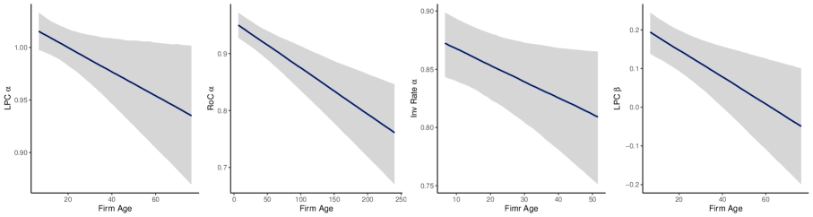
Figure 12: Marginal effects of Firm Age on $\alpha$ of labor productivity change ($\Delta LP$), profitability ($ROC$), and investment rate $IR$, and $\beta$ of $\Delta LP$. The blue line is the mean estimate and the grey shade area is the 90% uncertainty interval.

The higher the average firm age, the lower $\alpha$ and thus heavier tails in $\Delta LP$, profitability, and Investment rate, and the lower $\beta$ in $\Delta LP$. $\gamma$ and $\delta$ are very noisy in all parameters except for $\gamma$ in profitability and investment rate. Figure 12 shows the marginal effects of firm age on key parameters. From this, we can infer that, when the province has a higher average firm age, 1) the market tends to be less competitive for technological change, profitability, and firm growth (a low $\alpha$ in $\Delta LP$, profitability, and investment rate), 2) the economy has an increasing number of less innovative firms (a low $\beta$ in $\Delta LP$), and 3) the firm performance in terms of profitability and investment tends to be diverse but with a relatively high degree of uncertainty.

Employment

:

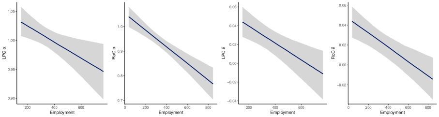
Figure 13: Marginal effects of Employment on $\alpha$ and $\delta$ of labor productivity change ($\Delta LP$) and profitability ($ROC$). The blue line is the mean estimate and the grey shade area is the 90% uncertainty interval.

A larger average employment size is associated with a lower $\alpha$ in $\Delta LP$, $LP$, profitability, a lower $\beta$ in profitability, a lower $\gamma$ in $\Delta LP$, $LP$, and a lower $\delta$ in $\Delta LP$ and Profitability. Investment Rate has a somewhat different pattern and has a positive relationship between employment size and $\alpha$ and $\delta$. Figure 13 shows the marginal effects of employment on key parameters. From this, we can infer that, when the province has larger size firms with a high number of employees, 1) the market tends to become less competitive overall (a low $\alpha$ in $\Delta LP$, $LP$, profitability), 2) firms become less technologically dynamic and more profitable (a low $\delta$ in $\Delta LP$ and profitability), and 3) firms become less diverse in their performance in technological change (a low $\gamma$ in $\Delta LP$ and $LP$).

Capital Intensity

:

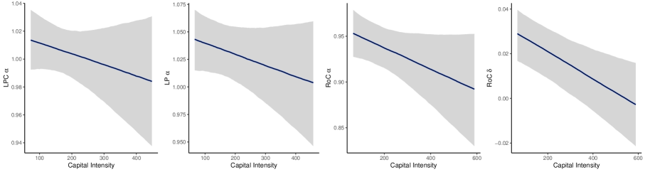
Figure 14: Marginal effects of Capital Intensity on $\alpha$ of labor productivity change ($\Delta LP$), $LP$, Returns on Capital, and $\delta$ of Returns on Capital. The blue line is the mean estimate and the grey shade area is the 90% uncertainty interval.

Higher average capital intensity is associated with a lower $\alpha$ in $\Delta LP$, $LP$, and Profitability but a higher $\alpha$ in the Investment rate, a higher $\gamma$ in $\Delta LP$ and $LP$, and a lower $\delta$ in profitability. Figure 14 shows the marginal effects of capital intensity on key parameters. From this, we can infer that, as the province has more firms with a higher capital intensity (a higher degree of mechanization), 1) the market tends to become less competitive overall (a low $\alpha$ in $\Delta LP$, $LP$, profitability), 2) firms become more diverse in their performance in technological change (a high $\gamma$ in $\Delta LP$ and $LP$), and 3) the firms tend to be less profitable overall (a low $\delta$ in profitability).

6 Conclusion

The distribution of productivity at the firm level has, like other economic quantities, been thoroughly investigated in recent years. For the developed economies, many stylized facts are known now: The distribution is unimodal, strongly right-skewed, has heavy tails, and is persistent in time. Yang et al. (2019), who also summarize the state of the art, report no systematic changes in their study covering millions of observations for European developed countries over a period of 10 years.

It is a fair question to ask if we might have systematic changes in developing countries, since these countries experience more rapid structural, demographic, and technological changes. Is the distribution the same? Do the parameter estimates show any trends? If so, what does that tell us about the development process and about development policy? Can and should productivity distributions be managed?

While we cannot provide direct evidence for the entire developing world, we did offer evidence for one country, the PR China as an example in this paper. Our study covers a crucial period of Chinese history, 1998-2007 (and further to 2013 with less reliable data), a period in which the country experienced the highest growth rates; when the economy and the technology sector took off; when the Chinese converged to the consumption and lifestyle habits of the developed world.

We demonstrated that the distributions of a wide range of quantities at the firm-level are heavy-tailed with a Lévy alpha-stable distribution being an excellent distributional model and clearly superior to the alternative AEP distribution that was also tested. This includes labor productivity ($LP$) and labor productivity change ($\Delta LP$). Consistent with the developed economies, both the shape of the distribution and the parameter values were remarkably consistent over time.

However, we did find a systematic shift: The location parameter of both productivity and productivity change were steadily increasing over the period of the study. The scale parameter $\gamma$ followed suit. Tail index ($\alpha$) and skew ($\beta$) were stable for the productivity level, but for the productivity change, the tail grew shorter ($\alpha$ increasing) and the distribution developed a right skew ($\beta$ increasing). What this means is that the productivity gains China experienced in the period of study do not come from super-star firms of exceptionally high productivity: The tail weight of $LP$ remained unchanged and that of $\Delta LP$ decreased. Instead, labor productivity increases became more consistent, concentrated, and uniform across the economy (decreasing tail weight of $\Delta LP$) and the body of labor productivity change extended to the right (emerging right-skew).

Further, we showed that there are significant and systematic differences across the regions of China that persist in time over the period of the study. This is even the case for differences for superficially similar regions such as the technology centers of Guangdong and Zhejiang/Shanghai. If this can be shown for the regions of China, that are subject to similar policies, environmental factors, and idiosyncratic shocks, differences in cross-country studies with multiple developing countries would be expected to be more pronounced.

Nevertheless, there were systematic relations between the parameters of the productivity distribution, a range of other distributions of micro-level variables (profitability, capital intensity, firm age), as well as macro-level characteristics (GDP growth, employment) of the respective regions, as shown in our Bayesian multi-level regression in Section 5.4.

The tail indices of the distributions were found to be between $\alpha=0.9$ and $\alpha=1.2$ in most cases, implying infinite variance (since $\alpha<2$) and very slow convergence to the theoretical mean, if the mean even exists (only for $\alpha\geq 1$). As a consequence, characteristics of the labor productivity distribution in the form of moments would be avoided. Such characteristics are, however, commonly given as variants of direct moments, the mean for the location, the variance, standard deviation, or Olley-Pakes gap for the dispersion. Hsieh and Klenow (2009) for instance, in his otherwise exemplary study of misallocation in China and India, uses sample variances.

What does this mean for development policy? First, concentration on super-star firms - be that domestic ones or branches of foreign groups - might be the wrong approach for successful technological catch-up. It would certainly be a different approach from that taken in China. Second, it instead seems important to ensure that productivity gains can also be realized by other firms. The most direct approach for this is encouraging technology transfer and providing incentives for sourcing intermediate products locally (which would also lead to cooperation and technology transfer). Technologies are arguably the most important factor in determining productivity at the firm level. Third, other factors such as instrumental institutions and a comprehensive education system could support this process. Fourth, significant differences would be expected between different countries. Direct comparisons of the parameters of productivity distributions in isolation are likely of only limited value. Instead, such comparisons should be done with a range of measures for the economic micro-structure at the firm level (productivity, age, capital intensity, etc.) while also taking the intertemporal development of these variables into account. Fifth, particular skepticism is advised with respect to measures that rely on moments of the productivity distribution (or similar quantities), as these may not exist. An example is the use of variance as a dispersion indicator, which will certainly fail.

While our findings are encouraging, more research is needed to confirm our findings for other developing countries. Do firm-level data in India, Vietnam, Nigeria, and other rapidly developing countries have the same characteristics? Can catch-up processes like the one showcased here be repeated in still other developing economies in the future? What impact might the Covid-19 pandemic have, that changed the face of the world economy by hitting many developed economies, but also some individual developing countries (like Tanzania) very hard?

Finally, can our example teach us something about the development history of European and other developed countries, the USA, Japan, South Korea? These countries’ catch-up phases were much longer ago in history, at a time, when economic microdata were not collected to the same extent as today. We may be unable to reconstruct the microdata, but it may still be possible to infer how the development process unfolded.

Appendix A Technical explanation of aggregation, maximum entropy, and distributional models

A.1 Aggregation and maximum entropy distributions

The form of aggregation of random variable distributions that is typically considered is convolution, i.e. the summation of random processes. For a defense why convolution is a suitable form of aggregation, see Frank (2009).

The sum of $n$ independent and identically distributed (i.i.d.) random variables $X_{1}+X_{2}+\ldots+X_{n}$. The distribution of (all) $X$ is an attractor distribution, if the aggregation converges to a distribution of the same form $X$. Formally (Nolan, 1998, 2019; Frank, 2009),

$$X_{1}+X_{2}+\ldots+X_{n}\sim c_{n}X+d_{n}$$ (6)

where $c_{n}$ and $d_{n}$ are scalars dependent on the number of convoluted distributions $n$. Such a distribution is called a stable distribution. The general form of stable distributions, Lévy alpha-stable distributions, are a generalization of Gaussian, Cauchy, and other specific distributions. We will consequently work with Lévy alpha-stable distributions as our distributional model for labor productivities and other firm-level variables in this paper.

Before we discuss the form, properties, and parametrizations of the Lévy alpha-stable distribution, we will give some background on aggregation and convergence to the entropy maximizing distribution under aggregation. Intuitively, aggregation leads to a loss of information; it washes out less strong signals and only a dominant pattern remains. As the convoluted distributions are independent, this pattern is the one that carries the least information (highest entropy), the one that is the most likely one without additional information, the one that constitutes the maximum entropy distribution under constraints that depend on the component distributions $X$.

For instance, constraints requiring a constant mean $\int_{-\infty}^{\infty}p(x)xdx=\mu$ and variance $\int_{-\infty}^{\infty}p(x)(x-\mu)dx=\sigma^{2}$ lead to a Gaussian as the entropy maximizing distribution. A constraint imposing a constant first moment (e.g., the mean) without constraints on the variance yields an exponential (one sided, constraint on mean, $\int_{0}^{\infty}p(x)xdx=\mu$) or Laplace distribution (two-sided with discontinuity, constraint on absolute deviation, $\int_{-\infty}^{\infty}p(x)(x-\mu)dx=a$). We will return to the constraint corresponding to the more general Lévy alpha-stable distribution in Section A.4.

It should be noted that not every maximum entropy distribution is a stable distribution, since the convolution of distributions $X$ may have an entropy maximizing distribution with a different functional form, which, in turn, may again aggregate to a distribution with another, different functional form.

A.2 The classical central limit theorem

The most well-known stable distribution is the Gaussian. This is known as the classical central limit theorem: Any sum over $n$ i.i.d. random variables with fixed mean and variance will converge to a Gaussian. The Gaussian is the solution to the entropy maximizing problem under this constraint (fixed variance, $(x-\mu)^{2}=\sigma^{2}$):

$$\Lambda=-\int_{-\infty}^{\infty}p(x)\log\left(\frac{p(x)}{m(x)}\right)dx-\lambda_{1}\left(\int_{-\infty}^{\infty}p(x)dx-1\right)-\lambda_{2}(p(x)(x-\mu)^{2}-\sigma^{2})$$ (7)

where the first term ($-\int_{-\infty}^{\infty}-p(x)\log(\frac{p(x)}{m(x)})dx$) is the entropy ($m(x)$ being the invariance measure), the second term the normalization constraint (probability must sum to $1$) and the last term the maximum entropy constraint. We obtain first-order conditions

$$\frac{\partial\Lambda}{\partial p(x)}=0=-\log\left(\frac{p(x)}{m(x)}\right)-1-\lambda_{1}-\lambda_{2}(x-\mu)^{2}$$

$$\frac{\partial\Lambda}{\partial\lambda_{1}}=0=\int_{-\infty}^{\infty}p(x)dx-1$$

$$\frac{\partial\Lambda}{\partial\lambda_{2}}=0=\int_{-\infty}^{\infty}p(x)(x-\mu)^{2}dx-\sigma^{2}$$

the first one of which directly yields the functional form of the density function $p(x)$ as

$$p(x)=me^{-\lambda_{1}}e^{-\lambda_{2}(x-\mu)^{2}}=ke^{-\lambda_{2}(x-\mu)^{2}}$$ (8)

where $k=me^{-\lambda_{1}}$ and $\lambda_{2}$ are constants. The values of these constants can be determined by substituting the function of $p(x)$ into the other two first-order conditions and solving. We then obtain $k=\frac{1}{\sigma\sqrt{2\pi}}$ and $\lambda_{2}=\frac{1}{2\sigma^{2}}$ and finally the Gaussian

$$p(x)=\sqrt{\frac{1}{2\pi\sigma^{2}}}e^{-\frac{1}{2\sigma^{2}}(x-\mu)^{2}}.$$ (9)

A.3 Fourier domain representations of random variable distributions

Distributions can also be represented as characteristic functions $\varphi(t)$ in the Fourier domain. While density $p(x)$ in the direct domain $x$ gives probabilities of realizations of values $x$, $\varphi(s)$ gives the intensity of fluctuations of frequencies $s$ in frequency space. If both functions, $p(x)$ and $\varphi(s)$, exist in functional form, there is a bijective mapping (a unique, invertible, one-to-one mapping) between the two, the Fourier transform

$$\varphi(s)=\operatorname{E}[e^{(isx)}]=\int_{-\infty}^{\infty}e^{(isx)}p(x)dx$$ (10)

where $\operatorname{E}$ represents the expectation. The inverse operation (inverse Fourier transform) is

$$p(x)=\frac{1}{2\pi}\int_{-\infty}^{\infty}e^{(-isx)}\varphi(s)ds.$$ (11)

However, in some cases, as for Lévy alpha-stable distributions, there is no functional representation of the density in the direct domain $p(x)$ and only the characteristic function $\varphi(s)$ in the Fourier domain exists.

Since the two representations are absolutely equivalent, the maximum entropy distribution can equivalently be obtained in Fourier domain.

Let $\varphi^{\prime}(s)$ be the normalized characteristic function. We apply entropy $S$ and entropy constraints $f_{i}(s)$ just like in the direct domain and maximize

$$\Lambda=S-\sum_{i}\lambda_{i}\int_{-\infty}^{\infty}f_{i}(s)\varphi^{\prime}(s)ds=-\int_{-\infty}^{\infty}\varphi^{\prime}(s)\log\left(\frac{\varphi^{\prime}(s)}{M(s)}\right)ds-\sum_{i}\lambda_{i}\int_{-\infty}^{\infty}f_{i}(s)\varphi^{\prime}(s)ds$$ (12)

with first-order conditions

$$\frac{\partial\Lambda}{\partial\varphi(s)}=0=-\log\left(\frac{\varphi^{\prime}(s)}{M(s)}\right)-1-\sum_{i}\lambda_{i}f_{i}(s)$$

$$\frac{\partial\Lambda}{\partial\lambda_{i}}=0=\int_{-\infty}^{\infty}f_{i}(s)\varphi^{\prime}(s)ds.$$

From the first condition, we obtain the general functional form of the maximum entropy distribution in the Fourier domain

$$\varphi^{\prime}(s)=M(s)e^{-1}e^{-\sum_{i}\lambda_{i}f_{i}(s)}=ke^{-\sum_{i}\lambda_{i}f_{i}(s)}.$$ (13)

where $k$ and $\lambda_{1}$ are factors that must be fixed by solving the other first-order conditions.

Returning to the example of the Gaussian above, we obtain the characteristic function of the same distribution (that we would also get by taking the Fourier transform of the density function in the direct domain) if we set the same constraint. Recall that for the Gaussian, this constraint is to fix the variance. In the Fourier domain, this is $s^{2}=\chi$. Hence, we substitute $f=s^{2}-\chi$ in equation 12 and after $\chi$ drops out in the derivative we obtain

$$\varphi^{\prime}(s)=ke^{-\lambda s^{2}},$$ (14)

or, more generally,

$$\varphi^{\prime}(s)=ke^{-\lambda(s^{\alpha}-\chi)}\quad\quad\quad\textup{ with }\alpha=2.$$ (15)

A.4 Lévy alpha-stable distributions

Instead of fixing the second moment, the variance, $\alpha=2$, as $\chi=s^{\alpha}=s^{2}$, the constraint can fix lower-order moments as the highest finite moments of the distribution. These moments do not need to be integer moments (fractional lower-order moments). They will, in fact, not be integers, except in case $\alpha=1$ (the Cauchy distribution). The computation of the maximum entropy distribution is equivalent, as long as we impose that the distribution is symmetric, $\beta=0$, and centered around zero, $\delta=0$. Analogous to equation 14, the distribution is now

$$\varphi^{\prime}(s)=ke^{-\lambda s^{\alpha}}.$$ (16)

For $\alpha<2$, $\varphi^{\prime}(s)$ does not have a functional representation in the direct domain any longer (except again for the Cauchy distribution, $\alpha=1$). The tails of the distribution do, however, asymptotically approach the power law

$$p_{Tail}(x)=C|x|^{-(\alpha+1)}.$$ (17)

and the distribution consequently has fat tails instead of quickly dropping to zero as in the Gaussian case with $\alpha=2$.

For the general case, without imposing symmetry and central location at zero, the characteristic equation becomes more complex and has four parameters, interpreted as the tail index ($\alpha$), the skew ($\beta$), the scale ($\gamma$), and the location ($\delta$). The functional form is

$$\varphi(s)=\operatorname{E}[e^{(isx)}]={\begin{cases}e^{(-\gamma^{\alpha}|s|^{\alpha}[1+i\beta\text{tan}\left({\tfrac{\pi\alpha}{2}}\right)\operatorname{sgn}(s)\left((\gamma|s|)^{1-\alpha}-1\right))]+i\delta s)}&\alpha\neq 1\\ e^{(-\gamma|s|[1+i\beta{\tfrac{2}{\pi}}\operatorname{sgn}(s)\log(\gamma|s|)]+i\delta s)}&\alpha=1\end{cases}}$$ (18)

More technical details on Lévy alpha-stable distributions can be found in Nolan (1998, 2019); a comprehensive discussion of maximum entropy, aggregation of distributions, and characteristic equations in the Fourier domain is offered in Frank (2009).

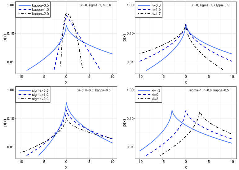
Figure 15: Density of the Asymmetric Exponential Power (AEP) distribution for different parameter settings. Upper left: Variation of tail parameter $\kappa$. Upper right: Variation of skew parameter $h$. Lower left: Variation of scale parameter $\sigma$. Lower right: Variation of location parameter $\xi$.

A.5 Asymmetric exponential power (AEP) distributions

For the distribution of the growth rates at the firm-level, the model advanced by Bottazzi and Secchi (2006); Bottazzi et al. (2007); Bottazzi and Secchi (2011) is considered a strong candidate, the asymmetric exponential power (AEP) or Subbotin distribution. This model is of particular interest here as an alternative model for comparison, since growth rates must be expected to be related to productivities in general, and to the labor productivity in particular. Firms with high labor productivity will generally have good prospects for future growth, while firms with low labor productivity will likely write losses and be unable to grow or even sustain their present operations unless supported by an inflow of additional resources.

The AEP is a generalization of the symmetric Laplace distribution, the two-sided exponential distribution. Bottazzi and Secchi (2006) take a very similar approach to the one taken in this paper: They characterize the distribution of growth as constant in mean absolute differences, use this as entropy constraint $|x-\xi|=\sigma$ and compute the maximum entropy distribution.

$$\Lambda=-\int_{-\infty}^{\infty}p(x)\log\left(\frac{p(x)}{m(x)}\right)dx-\lambda_{1}\left(\int_{-\infty}^{\infty}p(x)dx-1\right)-\lambda_{2}(p(x)|x-\xi|-\sigma)$$ (19)

The first-order condition with respect to $p(x)$

$$\frac{\partial\Lambda}{\partial p(x)}=0=-\log\left(\frac{p(x)}{m(x)}\right)-1-\lambda_{1}-\lambda_{2}|x-\xi|$$

yields the functional form

$$p(x)=me^{-\lambda_{1}}e^{-\lambda_{2}|x-\xi|}=ke^{-\lambda_{2}|x-\mu|}.$$ (20)

Solving the remaining first-order conditions (not given here) fixes parameters $k$ and $\lambda_{2}$ and results in the canonical form of the standard Laplace distribution,

$$p(x)=\frac{1}{2\sigma}e^{-\frac{|x-\xi|}{\sigma}}.$$ (21)

Relaxing the assumptions on symmetry and tail behavior yields the more general functional form of the AEP,

$$p(x)=\frac{\kappa h}{\sigma(1+\kappa^{2})\Gamma(1/h)}e^{[-(\kappa^{\operatorname{sgn}(x-\xi)}(|x-\xi|/\sigma))^{h}}$$ (22)

where $\Gamma$ is the Gamma function. The given parametrization is for the 4-parameter AEP that we will use as an alternative model and point of comparison in Section 5. The four parameters again stand for the tail behavior ($\kappa$), the skew ($h$), the scale ($\sigma$), and the location ($\xi$) and are visualized in the four panels of Figure 15 in direct comparison to the Lévy alpha-stable distribution in Figure 2. Again, the diagrams are in semi-log scale with the vertical axis being logarithmic. As expected, all AEP variants approach a linear shape towards both tails in the semi-log form, indicating that they belong to the family of exponential distribution forms (which are linear in semi-log). In contrast, the Lévy alpha-stable functions above bend in outward direction and clearly have tails that are heavier than exponential.

As an alternative to the 4-parameter AEP, there is a 5-parameter variant, which assigns two different tail parameters for positive and negative tails. We choose to work with the 4-parameter version to allow a more direct comparison with the 4-parameter Lévy alpha-stable function under consideration here.

A.6 Tail behavior

While the AEP results as the maximum entropy distribution for specific conditions, it is not a stable distribution: Summing AEPs will yield a Gaussian aggregate. While the difference may seem academic when considering the very similar body part of the distributions in Figures 2 and 15, the difference becomes important with the tail behavior and the finiteness of moments: In the case of Lévy alpha-stable distributions with $\alpha<2$, the variance is infinite. That is, each sample will have a specific variance, but the sample variance will diverge in sample size $N$ (Nolan, 2019; Emberchts et al., 1997; Yang et al., 2019) with

$$Var(x)\sim N^{\frac{2-\alpha}{2\alpha}}.$$ (23)

The mean of the distribution may or may not (if $\alpha<1$) be finite. But as the expected deviation from the mean is infinite, the information carried by each observation about the true mean is practically zero. The mean, albeit existent, may be difficult or impossible to infer from a sample.

This is not to say that nothing can be known for sure about Lévy alpha-stable distributed samples. On the contrary, both the quantiles of the distribution and its fitted parameters will converge and convey everything there is to know about the distribution. It is merely a matter of choosing the correct interpretation of the data and using adequate measures to characterize it.

Appendix B Prior specification of the regression model

The likelihood function and the priors of a Bayesian multi-level model in section 5.4 are written as follows:

$$\operatorname{Parameter_{i}} \sim \operatorname{Normal}(\mu_{i},\sigma)$$

$$\mu_{i} = \alpha+\alpha_{{}_{j[i]}}+\alpha_{{}_{t[i]}}+\beta_{1}\operatorname{GDP\_Growth}+\beta 2\operatorname{Firm\_Age}+\beta 3\operatorname{Emp}+\beta 4\operatorname{Cap\_Intensity}$$

$$\alpha \sim \operatorname{Student-t}(3,1,10)$$

$$\beta_{1},\beta_{2},\beta_{3},\beta_{4} \sim \operatorname{Normal}(0,1)$$

$$\sigma \sim \operatorname{Student-t}^{+}(3,0,10)$$

$$\alpha_{{}_{j}} \sim \operatorname{Normal}(\mu_{j},\sigma_{j})$$

$$\alpha_{{}_{t}} \sim \operatorname{Normal}(\mu_{t},\sigma_{t})$$

$$\mu_{j},\mu_{t} \sim \operatorname{Normal}(0,1)$$

$$\sigma_{j},\sigma_{t} \sim \operatorname{HalfCauchy}(0,1)$$

From line 3, we define the prior distribution for each parameter of the model. The overall intercept (the grand mean), $\alpha$ is given a weakly informative prior in the form of the Student’s-t distribution centered on 1 with 3 degrees of freedom and 10 standard deviation. The population effect coefficients, $\beta_{1},\beta_{2},\beta_{3},\beta_{4}$, are given a Gaussian prior centered on 0 with 1 standard deviation. The standard deviation of the Gaussian likelihood function, $\sigma$, is given a weak prior in the form of the half Student’s-t distribution centered on 0 with 3 degrees of freedom and 10 standard deviation. The varying intercepts, $\alpha_{j[i]}$ and $\alpha_{t[i]}$ are given a Gaussian prior with a hierarchical structure. The hyperpriors on the mean, $\mu_{j}$ and $\mu_{t}$ are given a Gaussian prior centered on 0 with 1 standard deviation. The hyperpriors on the standard deviation, $\sigma_{j}$ and $\sigma_{t}$ are given a Half-Cauchy prior centered on 0 with scale parameter 1. Note that $\sigma_{\alpha_{t}}$ and $\sigma_{\alpha_{j}}$ represent the estimated between-year variance and the between-province variance, respectively. For a detailed discussion on the choice of prior in Bayesian statistics, see Gelman et al. (2017).

Appendix C Historical note on productivity growth in the PR China

What caused the period of rapid economic growth in the PR China? Since the economic reform was initiated in 1978, the PR China has undergone significant structural change (Brandt et al., 2008; Wu, 2011; Bosworth and Collins, 2008; Chow and Li, 2002) - going from an agricultural to an industrial economy with growing importance of the service-sector - and achieving many important milestones. The early period was dominated by productivity improvements in agriculture (notably with the transformation from the production-team system to household responsibility system (HRS) (Lin, 1992; McMillan et al., 1989). The rapid productivity growth in the agricultural sector - 6.5% annually on average while labor input in the primary sector declines 4.5-5.5 % annually (Cao and Birchenall, 2013; Borensztein and Ostry, 1996) - came to an end around 1984, because the slowing new labor participation and technology adoption after 1984, and the institutional change exhausted its catch-up potential (Lin, 1992). In turn, the industrial and service sectors absorbed the labor freed in the primary sector, while also being boosted by an increasing work participation rate (Lin, 1992) and improved education and human capital accumulation Au and Henderson (2006); Gordon and Li (1995). The 1980s saw a fundamental reform of the economic organization (enterprise reform) followed by increasing international investment in the PR China in the 1990s, which probably boosted economic growth through technology transfer and spillovers (Hu et al., 2005). In 2001, the PR China was admitted to the WTO, allowing better integration in the global economy with again a significant effect on economic growth (Brandt et al., 2017). By then, manufacturing was the workhorse of the Chinese economy, with productivity growth in manufacturing between 1998 and 2007 being estimated as 7.7% annually Brandt et al. (2012), of which two-thirds came from the productivity differences between entering and existing firms.

Firms in the PR China are typically categorized into seven types (Yu et al., 2015): (1) Traditional state-owned enterprises (SOE), (2) collective owned enterprises, in particular Township and village enterprises (TVE), (3) shareholding firms, (4) private firms, (5) Hong Kong, Macao, and Taiwan owned companies, (6) foreign-owned companies, and (7) other domestic firms. Up to the enterprise reform, the economy was dominated by the first two categories (SOEs and TVEs) with the first phase of growth and rising productivity in the 1980s being carried to a significant part by TVEs, before private ownership became legal with the enterprise reform (Goodhart and Xu, 1996; Ito, 2006; Jefferson and Rawski, 1994), which introduced categories (3) and (4). Categories (5) and (6) would only become important with the increasing international integration of the economy of the PR China in the 1990s and 2000s.

Appendix D Additional results

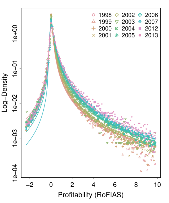
Figure 16: Density of the profitability (return on capital, $ROC$) distribution (full sample) by year in semi-log (vertical axis logarithmic). Solid lines indicate Levy alpha stable distribution fits as reported in Table 2.

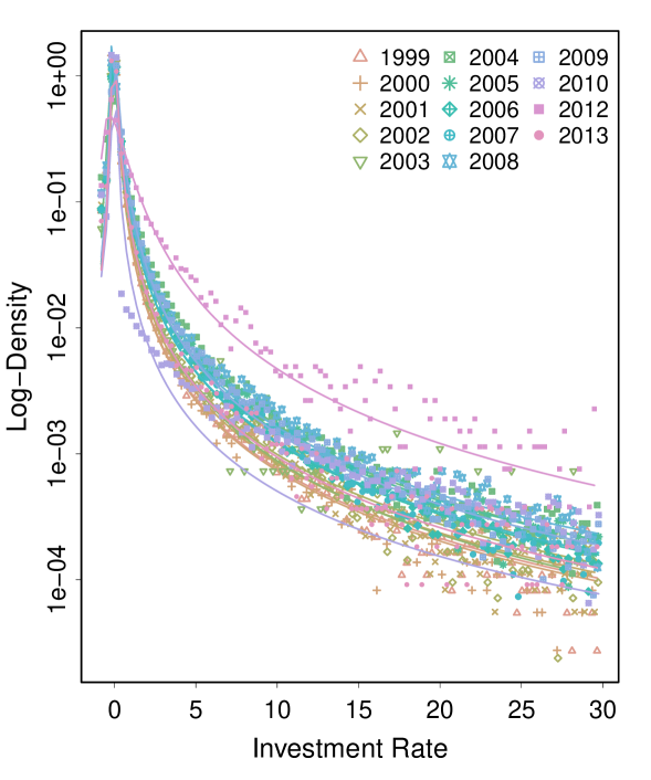
Figure 17: Density of the investment rate ($IR$) distribution (full sample) by year in semi-log (vertical axis logarithmic). Solid lines indicate Levy alpha stable distribution fits as reported in Table 2.

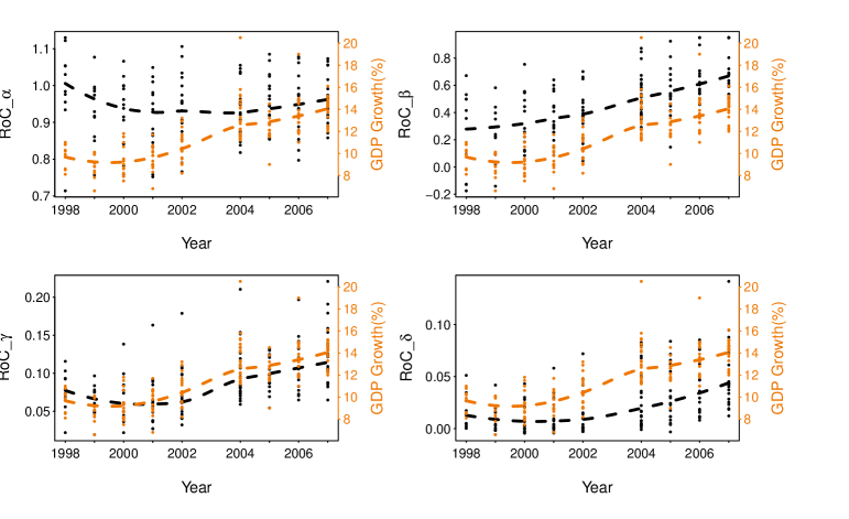
Figure 18: Return on capital by region and year (black) in comparison to GDP growth (orange).

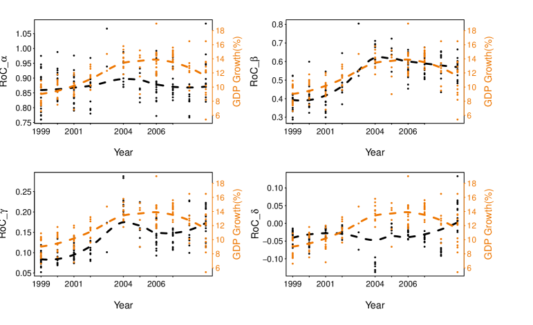
Figure 19: Investment rate by region and year (black) in comparison to GDP growth (orange).

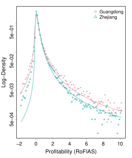
(a) $LP$

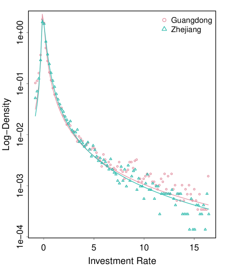
(b) $\Delta LP$

Figure 20: Density of $ROC$ and $IR$ for regions Guangdong and Zhejiang in 2007

Variable	Coefficient	$\alpha$				$\beta$				$\gamma$				$\delta$
		Est.	SE	CI 5%	CI 95%	Est.	SE	CI 5%	CI 95%	Est.	SE	CI 5%	CI 95%	Est.	SE	CI 5%	CI 95%
LP Change	Intercept	0.984	0.046	0.894	1.075	-0.056	0.102	-0.26	0.151	0.055	0.047	-0.033	0.143	-0.011	0.024	-0.056	0.037
	GDP Growth	0.008	0.003	0.003	0.013	0.026	0.007	0.013	0.038	0.009	0.003	0.004	0.014	0.005	0.001	0.003	0.008
	Firm.Age	-0.001	0.001	-0.002	0	-0.003	0.001	-0.006	-0.001	0	0	-0.001	0.001	0	0	-0.001	0.001
	Employment	0	0	0	0	0	0	0	0	0	0	0	0	0	0	0	0
	Cap Intensity	0	0	0	0	0	0	0	0	0	0	0	0.001	0	0	0	0
	sd(Class)	0.043	0.008	0.029	0.06	0.065	0.017	0.037	0.1	0.038	0.007	0.027	0.054	0.019	0.004	0.012	0.028
	sd(Year)	0.009	0.007	0	0.027	0.08	0.031	0.039	0.156	0.041	0.014	0.021	0.076	0.017	0.006	0.009	0.033
	WAIC	-586.565	30.229			-314.187	19.377			-681.084	30.577			-872.515	54.299
LP	Intercept	1.082	0.051	0.981	1.178	0.917	0.017	0.883	0.948	0.23	0.063	0.112	0.355	0.257	0.068	0.123	0.396
	GDP Growth	0.001	0.003	-0.005	0.007	0.002	0.001	-0.001	0.004	0.005	0.003	-0.001	0.012	0.009	0.004	0.002	0.016
	Firm.Age	0	0	0	0	0	0	0	0	0	0	0	0	0	0	0	0
	Employment	0	0	0	0	0	0	0	0	0	0	-0.001	0	0	0	-0.001	0
	Cap Intensity	0	0	0	0	0	0	0	0	0	0	0	0.001	0	0	0	0
	sd(Class)	0.051	0.009	0.036	0.07	0.008	0.004	0.001	0.016	0.08	0.014	0.057	0.112	0.086	0.014	0.062	0.117
	sd(Year)	0.029	0.011	0.014	0.057	0.003	0.003	0	0.01	0.057	0.02	0.032	0.102	0.083	0.027	0.048	0.156
	WAIC	-577.335	20.28			-763.403	92.099			-626.065	39.083			-581.903	39.123
ROC	Intercept	1.124	0.056	1.009	1.227	0.167	0.134	-0.103	0.431	0.071	0.021	0.031	0.114	0.034	0.018	-0.002	0.068
	GDP Growth	-0.003	0.003	-0.01	0.003	0.033	0.008	0.017	0.049	0.003	0.001	0.001	0.006	0.002	0.001	0	0.004
	Firm.Age	-0.001	0	-0.001	0	0	0	-0.001	0.001	0	0	0	0	0	0	0	0
	Employment	0	0	0	0	0	0	-0.001	0	0	0	0	0	0	0	0	0
	Cap Intensity	0	0	0	0	0	0	0	0	0	0	0	0	0	0	0	0
	sd(Class)	0.046	0.009	0.031	0.066	0.164	0.028	0.118	0.232	0.029	0.005	0.022	0.04	0.017	0.003	0.012	0.024
	sd(Year)	0.024	0.011	0.009	0.053	0.127	0.046	0.063	0.24	0.02	0.007	0.01	0.038	0.016	0.006	0.008	0.031
	WAIC	-439.61	18.542			-275.578	20.391			-861.659	23.479			-869.361	32.042
Inv Rate	Intercept	0.795	0.049	0.703	0.89	0.42	0.096	0.234	0.604	0.122	0.029	0.066	0.179	-0.069	0.019	-0.107	-0.031
	GDP Growth	0	0.003	-0.005	0.006	0.005	0.004	-0.004	0.013	0.003	0.002	0	0.006	0	0.001	-0.002	0.002
	Firm.Age	-0.001	0.001	-0.003	0	0.001	0.002	-0.002	0.004	-0.001	0	-0.002	0	0	0	-0.001	0
	Employment	0	0	0	0	0	0	0	0	0	0	0	0	0	0	0	0
	Cap Intensity	0	0	0	0	0	0	0	0	0	0	0	0	0	0	0	0
	sd(Class)	0.058	0.011	0.04	0.083	0.06	0.016	0.034	0.094	0.02	0.004	0.013	0.029	0.011	0.002	0.007	0.016
	sd(Year)	0.032	0.01	0.018	0.057	0.193	0.052	0.117	0.322	0.046	0.013	0.029	0.078	0.04	0.01	0.026	0.065
	WAIC	-486.833	20.609			-326.147	37.232			-617.939	20.353			-754.725	31.133

Table 5: Detailed regression results

References

- Adamopoulos and Restuccia (2014) Adamopoulos, T. and Restuccia, D. (2014). The size distribution of farms and international productivity differences. American Economic Review, 104(6):1667–97.
- Akaike (1973) Akaike, H. (1973). Maximum likelihood identification of Gaussian autoregressive moving average models. Biometrika, 60(2):255–265.
- Angelini and Generale (2008) Angelini, P. and Generale, A. (2008). On the evolution of firm size distributions. American Economic Review, 98(1):426–38.
- Asquith (2018) Asquith, W. (2018). lmomco - L-moments, censored L-moments, trimmed L-moments, L-comoments, and many distributions. R package version 2.3.1.
- Asquith (2014) Asquith, W. H. (2014). Parameter estimation for the 4-parameter asymmetric exponential power distribution by the method of l-moments using r. Computational Statistics & Data Analysis, 71:955 – 970.
- Au and Henderson (2006) Au, C.-C. and Henderson, J. V. (2006). How migration restrictions limit agglomeration and productivity in China. Journal of Development Economics, 80(2):350–388.
- Axtell (2001) Axtell, R. L. (2001). Zipf distribution of U.S. firm sizes. Science, 293(5536):1818–1820.
- Bartelsman et al. (2013) Bartelsman, E., Haltiwanger, J., and Scarpetta, S. (2013). Cross-country differences in productivity: The role of allocation and selection. American Economic Review, 103(1):305–34.
- Beaudry and Schiffauerova (2009) Beaudry, C. and Schiffauerova, A. (2009). Who’s right, marshall or jacobs? the localization versus urbanization debate. Research Policy, 38(2):318 – 337.
- Berlingieri et al. (2017) Berlingieri, G., Blanchenay, P., and Criscuolo, C. (2017). The great divergence(s). OECD Science, Technology and Industry Policy Papers, 39.
- Bloom et al. (2010) Bloom, N., Mahajan, A., McKenzie, D., and Roberts, J. (2010). Why do firms in developing countries have low productivity? American Economic Review, 100(2):619–23.
- Boeing et al. (2016) Boeing, P., Mueller, E., and Sandner, P. (2016). China’s R&D explosion - analyzing productivity effects across ownership types and over time. Research policy, 45(1):159–176.
- Borensztein and Ostry (1996) Borensztein, E. and Ostry, J. D. (1996). Accounting for China’s growth performance. The American Economic Review, 86(2):224–228.
- Bosworth and Collins (2008) Bosworth, B. and Collins, S. M. (2008). Accounting for growth: comparing China and India. Journal of Economic Perspectives, 22(1):45–66.
- Bottazzi et al. (2007) Bottazzi, G., Cefis, E., Dosi, G., and Secchi, A. (2007). Invariances and diversities in the patterns of industrial evolution: Some evidence from italian manufacturing industries. Small Business Economics, 29(1-2):137–159.
- Bottazzi and Secchi (2006) Bottazzi, G. and Secchi, A. (2006). Explaining the distribution of firm growth rates. The RAND Journal of Economics, 37(2):235–256.
- Bottazzi and Secchi (2011) Bottazzi, G. and Secchi, A. (2011). A new class of asymmetric exponential power densities with applications to economics and finance. Industrial and corporate change, 20(4):991–1030.
- Brandt et al. (2008) Brandt, L., Hsieh, C.-T., and Zhu, X. (2008). Growth and structural transformation in China. In Brandt, L. and Rawski, T. G., editors, China’s Great Economic Transformation, page 683–728. Cambridge University Press.
- Brandt et al. (2017) Brandt, L., Van Biesebroeck, J., Wang, L., and Zhang, Y. (2017). Wto accession and performance of chinese manufacturing firms. American Economic Review, 107(9):2784–2820.
- Brandt et al. (2012) Brandt, L., Van Biesebroeck, J., and Zhang, Y. (2012). Creative accounting or creative destruction? firm-level productivity growth in chinese manufacturing. Journal of Development Economics, 97(2):339–351.
- Brandt et al. (2014) Brandt, L., Van Biesebroeck, J., and Zhang, Y. (2014). Challenges of working with the chinese nbs firm-level data. China Economic Review, 30:339–352.
- Bürkner (2017) Bürkner, P.-C. (2017). brms: An R package for Bayesian multilevel models using Stan. Journal of Statistical Software, 80(1):1–28.
- Cabral and Mata (2003) Cabral, L. M. B. and Mata, J. (2003). On the evolution of the firm size distribution: Facts and theory. American Economic Review, 93(4):1075–1090.
- Cao and Birchenall (2013) Cao, K. H. and Birchenall, J. A. (2013). Agricultural productivity, structural change, and economic growth in post-reform China. Journal of Development Economics, 104:165–180.
- Carpenter et al. (2017) Carpenter, B., Gelman, A., Hoffman, M. D., Lee, D., Goodrich, B., Betancourt, M., Brubaker, M., Guo, J., Li, P., and Riddell, A. (2017). Stan: A probabilistic programming language. Journal of statistical software, 76(1).
- Carrasco et al. (2007) Carrasco, M., Florens, J.-P., and Renault, E. (2007). Linear inverse problems in structural econometrics estimation based on spectral decomposition and regularization. Handbook of econometrics, 6:5633–5751.
- Chaffai et al. (2012) Chaffai, M., Kinda, T., and Plane, P. (2012). Textile manufacturing in eight developing countries: Does business environment matter for firm technical efficiency? The Journal of Development Studies, 48(10):1470–1488.
- Chen et al. (2009) Chen, K.-H., Huang, Y.-J., and Yang, C.-H. (2009). Analysis of regional productivity growth in China: A generalized metafrontier MPI approach. China Economic Review, 20(4):777–792.
- Chow and Li (2002) Chow, G. C. and Li, K.-W. (2002). China’s economic growth: 1952–2010. Economic Development and Cultural Change, 51(1):247–256.
- Chudnovsky et al. (2006) Chudnovsky, D., López, A., and Pupato, G. (2006). Innovation and productivity in developing countries: A study of argentine manufacturing firms’ behavior (1992–2001). Research Policy, 35(2):266 – 288.
- Coad and Tamvada (2012) Coad, A. and Tamvada, J. P. (2012). Firm growth and barriers to growth among small firms in india. Small Business Economics, 39(2):383–400.
- di Giovanni et al. (2011) di Giovanni, J., Levchenko, A. A., and Rancière, R. (2011). Power laws in firm size and openness to trade: Measurement and implications. Journal of International Economics, 85(1):42 – 52.
- Ding et al. (2016) Ding, S., Guariglia, A., and Harris, R. (2016). The determinants of productivity in chinese large and medium-sized industrial firms, 1998–2007. Journal of Productivity Analysis, 45(2):131–155.
- Emberchts et al. (1997) Emberchts, P., Kluppelberg, C., and Mikosch, T. (1997). Time series analysis for heavy-tailed processes. In Modelling Extremal Events,, pages 371–412. Springer, Berlin, Heidelberg.
- Fariñas and Ruano (2004) Fariñas, J. C. and Ruano, S. (2004). The dynamics of productivity: A decompostion approach using distribution functions. Small Business Economics, 22(3-4):237–251.
- Frank (2009) Frank, S. A. (2009). The common patterns of nature. Journal of Evolutionary Biology, 22(8):1563–1585.
- Fujimoto et al. (2011) Fujimoto, S., Ishikawa, A., Mizuno, T., and Watanabe, T. (2011). A new method for measuring tail exponents of firm size distributions. Economics: The Open-Access, Open-Assessment E-Journal, 5(1-20).
- Gabaix (2011) Gabaix, X. (2011). The granular origins of aggregate fluctuations. Econometrica, 79(3):733–772.
- Gaffeo et al. (2003) Gaffeo, E., Gallegati, M., and Palestrini, A. (2003). On the size distribution of firms: additional evidence from the G7 countries. Physica A: Statistical Mechanics and its Applications, 324(1-2):117 – 123. Proceedings of the International Econophysics Conference.
- Gelman et al. (2014) Gelman, A., Carlin, J. B., Stern, H. S., Dunson, D. B., Vehtari, A., and Rubin, D. B. (2014). Bayesian data analysis, volume 2. CRC press Boca Raton, FL.
- Gelman et al. (2017) Gelman, A., Simpson, D., and Betancourt, M. (2017). The prior can often only be understood in the context of the likelihood. Entropy, 19(10):555.
- Gong (2018) Gong, B. (2018). Agricultural reforms and production in China: Changes in provincial production function and productivity in 1978–2015. Journal of Development Economics, 132:18–31.
- Goodhart and Xu (1996) Goodhart, C. and Xu, C. (1996). The rise of China as an economic power. National Institute Economic Review, 155(1):56–80.
- Gordon and Li (1995) Gordon, R. H. and Li, W. (1995). The change in productivity of chinese state enterprises, 1983–1987. Journal of Productivity Analysis, 6(1):5–26.
- Goyette and Gallipoli (2015) Goyette, J. and Gallipoli, G. (2015). Distortions, efficiency and the size distribution of firms. Journal of Macroeconomics, 45:202 – 221.
- Groves et al. (1994) Groves, T., Hong, Y., McMillan, J., and Naughton, B. (1994). Autonomy and incentives in chinese state enterprises. The Quarterly Journal of Economics, 109(1):183–209.
- Hansen (1982) Hansen, L. P. (1982). Large sample properties of generalized method of moments estimators. Econometrica, 50(4):1029–1054.
- Heinrich and Dai (2016) Heinrich, T. and Dai, S. (2016). Diversity of firm sizes, complexity, and industry structure in the Chinese economy. Structural Change and Economic Dynamics, 37:90 – 106.
- Heinrich et al. (2020) Heinrich, T., Yang, J., and Dai, S. (2020). Levels of structural change: An analysis of china’s development push 1998-2014. OMPTEC Working Paper No. 2020-4, Oxford Martin School, University of Oxford, arXiv preprint arXiv:2005.01882, https://www.oxfordmartin.ox.ac.uk/publications/levels-of-structural-change-an-analysis-of-chinas-development-push-1998-2014/.
- Hsieh and Klenow (2009) Hsieh, C.-T. and Klenow, P. J. (2009). Misallocation and manufacturing TFP in China and India. The Quarterly Journal of Economics, 124(4):1403–1448.
- Hsieh and Song (2015) Hsieh, C.-T. and Song, Z. M. (2015). Grasp the large, let go of the small: The transformation of the state sector in China. Brookings Papers on Economic Activity, (1):295–346.
- Hu and Jefferson (2004) Hu, A. G. and Jefferson, G. H. (2004). Returns to research and development in chinese industry: Evidence from state-owned enterprises in beijing. China Economic Review, 15(1):86–107.
- Hu et al. (2005) Hu, A. G., Jefferson, G. H., and Jinchang, Q. (2005). R&d and technology transfer: firm-level evidence from chinese industry. Review of Economics and Statistics, 87(4):780–786.
- Ijiri and Simon (1964) Ijiri, Y. and Simon, H. A. (1964). Business firm growth and size. The American Economic Review, 54(2):77–89.
- Ijiri and Simon (1977) Ijiri, Y. and Simon, H. A. (1977). Skew distributions and the sizes of business firms, volume 24. North Holland, Amsterdam.
- Ito (2006) Ito, J. (2006). Economic and institutional reform packages and their impact on productivity: A case study of chinese township and village enterprises. Journal of Comparative Economics, 34(1):167–190.
- Jefferson and Rawski (1994) Jefferson, G. H. and Rawski, T. G. (1994). Enterprise reform in chinese industry. Journal of economic perspectives, 8(2):47–70.
- Jefferson et al. (2000) Jefferson, G. H., Rawski, T. G., Li, W., and Yuxin, Z. (2000). Ownership, productivity change, and financial performance in chinese industry. Journal of Comparative Economics, 28(4):786–813.
- Jiang (2011) Jiang, Y. (2011). Understanding openness and productivity growth in China: An empirical study of the chinese provinces. China Economic Review, 22(3):290–298.
- Kharrat and Boshnakov (2016) Kharrat, T. and Boshnakov, G. N. (2016). StableEstim: Estimate the Four Parameters of Stable Laws using Different Methods. R package version 2.1.
- Li and Rama (2015) Li, Y. and Rama, M. (2015). Firm Dynamics, Productivity Growth, and Job Creation in Developing Countries: The Role of Micro- and Small Enterprises. The World Bank Research Observer, 30(1):3–38.
- Lin (1992) Lin, J. Y. (1992). Rural reforms and agricultural growth in China. The American economic review, pages 34–51.
- Ma et al. (2008) Ma, Q., Chen, Y., Tong, H., and Di, Z. (2008). Production, depreciation and the size distribution of firms. Physica A: Statistical Mechanics and its Applications, 387(13):3209 – 3217.
- McCulloch (1986) McCulloch, J. H. (1986). Simple consistent estimators of stable distribution parameters. Communications in Statistics-Simulation and Computation, 15(4):1109–1136.
- McMillan et al. (1989) McMillan, J., Whalley, J., and Zhu, L. (1989). The impact of China’s economic reforms on agricultural productivity growth. Journal of Political Economy, 97(4):781–807.
- Mitzenmacher (2004) Mitzenmacher, M. (2004). A brief history of generative models for power law and lognormal distributions. Internet Mathematics, 1(2):226–251.
- Nguyen (2019) Nguyen, D. X. (2019). Minimum wages and firm productivity: Evidence from vietnamese manufacturing firms. International Economic Journal, 33(3):560–572.
- Nolan (1998) Nolan, J. P. (1998). Parameterizations and modes of stable distributions. Statistics & Probability Letters, 38(2):187 – 195.
- Nolan (2019) Nolan, J. P. (2019). Stable distributions - models for heavy tailed data. boston. Unfinished manuscript.
- Poschke (2018) Poschke, M. (2018). The firm size distribution across countries and skill-biased change in entrepreneurial technology. American Economic Journal: Macroeconomics, 10(3):1–41.
- Schwarzkopf et al. (2010) Schwarzkopf, Y., Axtell, R., and Farmer, J. D. (2010). An explanation of universality in growth fluctuations. Available at SSRN: https://ssrn.com/abstract=1597504.
- Song et al. (2011) Song, Z., Storesletten, K., and Zilibotti, F. (2011). Growing like China. American Economic Review, 101(1):196–233.
- Soofi et al. (1995) Soofi, E. S., Ebrahimi, N., and Habibullah, M. (1995). Information distinguishability with application to analysis of failure data. Journal of the American Statistical Association, 90(430):657–668.
- Stan Development Team (2015) Stan Development Team (2015). Rstan: the r interface to stan, version 2.8.0.
- Sun and Zhang (2012) Sun, C. and Zhang, T. (2012). Export, productivity pattern, and firm size distribution. (36742).
- Van Biesebroeck (2005) Van Biesebroeck, J. (2005). Firm size matters: Growth and productivity growth in african manufacturing. Economic Development and Cultural Change, 53(3):545–583.
- Volpe Martincus and Carballo (2010) Volpe Martincus, C. and Carballo, J. (2010). Beyond the average effects: The distributional impacts of export promotion programs in developing countries. Journal of Development Economics, 92(2):201 – 214.
- Wu (2011) Wu, Y. (2011). Total factor productivity growth in China: a review. Journal of Chinese economic and business studies, 9(2):111–126.
- Yang (2018) Yang, J. (2018). A quantal response statistical equilibrium model of induced technical change in an interactive factor market: Firm-level evidence in the eu economies. Entropy, 20(3).
- Yang et al. (2019) Yang, J., Heinrich, T., Winkler, J., Lafond, F., Koutroumpis, P., and Farmer, J. D. (2019). Measuring productivity dispersion: a parametric approach using the Lévy alpha-stable distribution. Working Paper, Oxford Martin School, University of Oxford, arXiv preprint arXiv:1910.05219, https://www.oxfordmartin.ox.ac.uk/publications/measuring-productivity-dispersion-a-parametric-approach-using-the-l%C3%A9vy-alpha-stable-distribution/.
- Yu et al. (2017) Yu, X., Dosi, G., Grazzi, M., and Lei, J. (2017). Inside the virtuous circle between productivity, profitability, investment and corporate growth: An anatomy of chinese industrialization. Research Policy, 46(5):1020–1038.
- Yu et al. (2015) Yu, X., Dosi, G., Lei, J., and Nuvolari, A. (2015). Institutional change and productivity growth in china’s manufacturing: the microeconomics of knowledge accumulation and ’creative restructuring’. Industrial and Corporate Change. forthcoming.
- Zhang et al. (2009) Zhang, J., Chen, Q., and Wang, Y. (2009). Zipf distribution in top chinese firms and an economic explanation. Physica A: Statistical Mechanics and its Applications, 388(10):2020 – 2024.
- Zhang and Liu (2013) Zhang, J. and Liu, X. (2013). The evolving pattern of the wage–labor productivity nexus in china: Evidence from manufacturing firm-level data. Economic Systems, 37(3):354 – 368.
- Zhu et al. (2019) Zhu, S., He, C., and Xia, X. (2019). Geography of productivity: evidence from China’s manufacturing industries. The Annals of Regional Science, 62(1):141–168.