Anisotropic magneto-thermal transport in Co₂MnGa thin films

Abstract

Ferromagnetic Co2MnGa has recently attracted significant attention due to effects related to non-trivial topology of its band structure, however a systematic study of canonical magneto-galvanic transport effects is missing. Focusing on high quality thin films, here we systematically measure anisotropic magnetoresistance (AMR) and its thermoelectric counterpart (AMTP). We model the AMR data by free energy minimisation within the Stoner–Wohlfarth formalism and conclude that both crystalline and non-crystalline components of this magneto-transport phenomenon are present in Co2MnGa. Unlike the AMR which is small in relative terms ($\sim 0.1\%$), the AMTP is large due to a change of sign of the Seebeck coefficient as a function of temperature. This fact is discussed in the context of the Mott rule and further analysis of AMTP components is presented.

Electron transport phenomena in magnetically ordered materials span a vast range both historically and from the point of view of complexity. While some of them which have been known for a long time, such as the anisotropic magnetoresistance (AMR) Thomson:1857_a , remain a subject of roughly constant interest until today Wang:2020_a ; Volny:2020_a ; Miao:2020_a others rose to prominence only recently. Such is the case of the anomalous Nernst effect Wesenberg:2018_a (ANE) for example, an outstanding member of the field of spin caloritronics Yu:2017_a . In a typical thin film geometry with magnetic field applied in the direction normal to the film plane and a thermal gradient in the sample plane, the ANE signal is detected in the other (perpendicular) in-plane direction. This effect is particularly strong in ferromagnetic Co2MnGa Hu:2020_a (identified as a Weyl semimetal Sakai2018 ) and having thus drawn considerable interest it has been investigated in sufficient detail already Reichlova2018 ; Belopolski2019 ; Park2020 .

In this work, we extend the discussion also to effects which occur when magnetic field is applied in the sample plane. The studied thin film of Heusler alloy Co2MnGa represents an ideal model system because of its high crystalline quality, relatively strong magneto-thermal response, its high Curie temperature ($T_{C}=694$ K) and high spin polarisation Graf:2011_a . We study systematically the magneto-thermal transport response when the magnetic field is rotated in three perpendicular rotation planes. Along with AMR, the anisotropic magneto-thermopower (AMTP) is reported and compared qualitatively. We discuss the applicability of a simple Stoner–Wohlfarth-based model (as used recently in a different context, for example in Ref. Volny:2020_a ) to the AMTP data and compare the ratio of amplitudes of AMTP and AMR in various samples and at different temperatures. We report crystalline contributions to both AMR and AMTP and interestingly, some of these seem missing (or at least they are significantly weaker) in the latter effect. Inconsistencies related to the straightforward application of the Mott rule to our measurements suggest a sizable phonon Protik:2020_a or magnon Polash:2020_a drag contribution to the thermopower.

This paper is structured as follows: in Sec I we are motivating the comparison of anisotropic magnetoresistance (AMR) and anisotropic magnetothermopower (AMTP) and provide some background on these two effects. In Sec II, the formalism used for the data analysis is introduced and sample fabrication and characterisation is described in Sec. III. Finally, experimental results are shown and discussed in Sec. IV; an outlook and and summary is provided in Sec. V.

I. INTRODUCTION

Both AMR and AMTP refer to voltage variation as a function of the angle between magnetization and the driving force (electrical current j in case of AMR and temperature gradient $\nabla T$ in case of AMTP) or the angle between magnetization and the crystal axes in the respective setting. Although they could probe similar physical properties, there are many more reports about AMR than about AMTP, mostly due to experimental challenges in measuring AMTP. In the following, we give a brief introduction of both.

Since the original observation of AMR by William Thomson Thomson:1857_a the AMR is typically understood as a variation of resistance as a function of magnetisation M direction Rushforth:2007_a $\Delta\rho_{yy}(\varphi)=C_{I}\cos 2\varphi$, with $\varphi$ denoting the angle between current and magnetisation. However, there is another level of complexity in AMR. In 1938, the discussion of this effect was extended to the influence of crystalline symmetry. W. Doering Doring:1938_a carried out symmetry-based AMR analysis Ranieri:2008_a of resistivity tensor using a series expansion up to fourth order in powers of the direction cosines of the magnetization. These expansions contain AMR terms different from the ”non-crystalline” $\cos 2\varphi$ ones and such additional terms are sometimes called ”crystalline” AMR since they reflect the crystal symmetry and not the symmetry breaking induced by the electrical current direction. Consequently, unlike the non-crystalline AMR, the crystalline AMR contributions can be non-zero even if $\varphi=\pi/2$ remains constant (for example, during the magnetic field rotation in the plane perpendicular to j. Such a situation will be discussed in the experimental setup sketched in Fig. 2(e) below.

AMTP is the thermoelectrical counterpart of AMR. The basic phenomenon (voltage drop induced by a temperature gradient) was discovered by T.J. Seebeck already in 1821, thus establishing the field of thermoelectrics. Hints at its anisotropy came much later Ky:1966_a however and since then, AMTP has attracted relatively small attention compared to the AMR. Nevertheless, increasing global demand for energetically sustainable solutions Snyder:2008 and the need of advanced microscopy techniques Janda:2020_b sparked new interest in this effect.

Recent thermoelectric studies in solid state magnetism focus mostly on the evaluation of $\Sigma$ (the Seebeck coefficient Loevvik:2020_a ) or the anomalous Nernst effect (ANE) Yu:2017_a . The Seebeck coefficient provides information about the charge carriers, such as concentration, effective mass or dominant type (electrons or holes) and ANE stirs interest due to the connection to band structure topology note2 and better technological prospects in thermoelectric energy harvesting Sakai2020 . In addition to the ANE, the Seebeck coefficient anisotropy comes with the possibility for its tensor components $\Sigma_{xy}$ and $\Sigma_{yy}$ to depend on the magnetic field direction: the anisotropic magneto-thermopower (AMTP) which is a direct analog to the non-crystalline AMR, can be expressed as

$$\Sigma_{\mathrm{xy}} = S_{I}\sin 2\varphi\qquad\mbox{ accompanied by }$$

$$\Delta\Sigma_{\mathrm{yy}} = S_{I}\cos 2\varphi,$$ (1)

where $\Delta\Sigma_{\mathrm{yy}}$ is the difference between $\Sigma_{yy}$ and its average. These relations pertinent to polycrystalline materials can be straightforwardly derived by angular averaging the Seebeck tensor as given by Eq. 3.31 in Ref. Limmer:2008_a and we also discuss this relationship in Sec. III.

In contrast to ANE, the AMTP is rarely a topic of systematic studies; with few exceptions Althammer:2012 ; Reimer:2017_a reports are usually limited to assume its existence (in longitudinal Jayathilaka:2015_a ; Janda:2020_a or transversal Ky:1966_a ; Avery:2012_a geometry also known as the planar Nernst effect) and the AMTP often assumes the role of an unwanted artefact. The main reasons are the notorious difficulty to precisely quantify direction and amplitude of a thermal gradient and small magnitude of the measured thermo-voltages, typically on resolution limit of a common laboratory equipment. This makes the AMTP experiment significantly more challenging than a simple resistivity measurement with a well-defined current direction. The thermal gradient quantification is even more complex in thin film samples where the substrate acts as a heat sink. The lack of detailed understanding of AMTP becomes obvious when considering systems with various contributions to AMR. In particular, very few reports show more complex symmetry of AMTP Althammer:2012 , the existence of a crystalline component in the AMTP is not yet established and a comparison between the crystalline contributions to AMR and AMTP is entirely missing. The understanding of AMTP is not only a fundamental scientific question, but it is equally important in order to exclude various artefacts in experiments during which thermal gradient is unintentionally generated.

II. SAMPLE FABRICATION AND CHARACTERIZATION

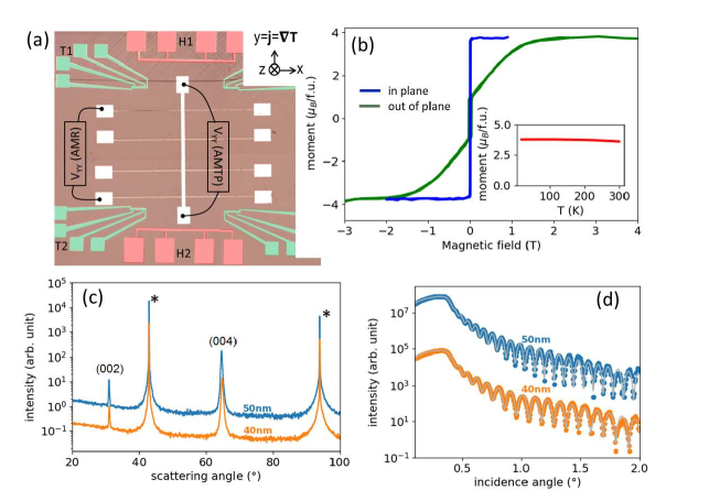
The Co₂MnGa thin-film samples are fabricated by magnetron sputtering on MgO(001) substrates using a multisource Bestec UHV deposition system from Co, Mn and MnGa sputter targets. Growth and post-growth annealing was performed at 500^∘C. After the Co₂MnGa thin-film growth, 3 nm of Al were deposited at room temperature to prevent oxidation. Further details of the growth procedure can be found elsewhere Markou:2019 . Here, two samples showing highest crystal quality with Co₂MnGa thickness of 40 nm and 50 nm are studied. The chemical composition and structural investigation conducted by X-ray diffraction techniques showed Bragg peaks corresponding to the material composition revealing a high degree of atomic order similar to Refs. Reichlova2018 ; Markou:2019 . Figure 1(c) shows the symmetric radial X-ray diffraction scans, which includes diffraction from lattice planes parallel to the substrate surface. Given the epitaxial alignment of Co₂MnGa(001)[110] $\parallel$ MgO(001)[100], i.e. an in-plane 45^∘ degree rotation, only the $00L$ Bragg peaks are visible in Fig. 1(c). Well defined, narrow Bragg peaks evidence the good chemical homogeneity and crystal quality. While bulk Co₂MnGa has a cubic L2₁ crystal structure the thin-films exhibit an epitaxial strain-induced tetragonal distortion with slight contraction along the out of plane [001] direction. Resulting $c/a$ ratio is around 0.99 Markou:2019 . Figure 1(d) shows X-ray reflectivity data of the 40 nm and 50 nm thick Co₂MnGa epilayer displaying Kiessig fringes that extend beyond the measurement range. This bears witness to a low surface and interface roughness which were determined to be below 7 Å by modelling using an extended Parratt formalism Pietsch:2004 .

Magnetization of these epilayers was measured in a SQUID magnetometer, which is shown in Fig. 1(b). The saturation magnetic moment of about 4 $\mu_{\mathrm{B}}$ / f.u. is consistent with literature (saturation magnetisation $M_{\mathrm{sat}}$ 720 kA/m) Reichlova2018 ; Park2020 . The films were patterned into 40$\mu$m wide Hall bars by optical lithography and by a combination of HCl and Ar/O2 plasma etching. A schematic image of the sample is shown in Fig. 1(a). After the etching, the heater and thermometers were fabricated in a lift-off process with 30 nm of sputtered Pt. Platinum wires, highlighted as pink areas in Fig. 1(a), at the top of the Hall bar serve as on-chip heater, while platinum wires at the side work as an on-chip thermometer (green areas).

Figure 1: Sample characterization. a) Schematic image of the sample. The white areas are Co2MnGa. $V_{\mathrm{xx}}$ (AMR) are the contacts used for measusing voltage in the AMR experiment, while the current $I$ was applied between $V_{\mathrm{xx}}$ (AMTP). In the AMTP experiment, the voltage was measured at $V_{\mathrm{xx}}$ (AMTP). The red colored areas are Pt wires which are used in the AMTP experiments as on-chip heater and thermometer (green). b) in-plane and out-of-plane measurement of the magnetization vs. applied magnetic field. The inset show the magnetization vs. temperature. The saturated magnetic moment is approx. $4\mu_{\mathrm{B}}$ per formula unit. c) X-ray diffraction radial scans of Co2MnGa films with 40 and 50nm thickness. Bragg peaks labeled by an asterisk (*) originate from the (00L) series of the MgO substrate, while Bragg peaks of Co2MnGa are labeled by their Miller indices. d) X-ray reflectivity pattern of the 40 nm and 50 nm thick Co2MnGa films. Experimental data are shown as data points, while the solid line represents a model fit based on the extended Parratt formalism.

Experimental Setup

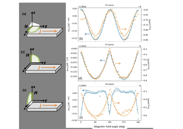
In the AMR experiments, a sufficiently strong magnetic field ($\mu_{0}H=1.5$ T stronger than $M_{\mathrm{sat}}\approx 0.9$ T and the anisotropy field $\approx 0.6$ T corresponding to $k_{u}$) is rotated in three rotation planes called XY, ZY and ZX plane as shown in Fig. 2 (a), (c) and (e). Current $I=0.2$ mA (corresponding to current density $1.2\times 10^{6}$ A/cm²) is applied along the y-axis. At each step of the magnetic field rotation, data is collected for $I=+0.2$ mA and for $I=-0.2$ mA and averaged, in order to cancel out the thermoelectric contributions, which occur in form of voltage offsets. The experiments are conducted at different temperatures between 10 K and 300 K. The data are shown as symbols in Fig. 2.

In the AMTP experiments, magnetic field is rotated in the same rotation planes XY, ZY and ZX. The experiments are conducted at several temperatures between 100 and 300 K; at lower temperatures the AMTP signal decreases below the resolution owing to the decrease of entropy.

The thermometers are first calibrated by sweeping the temperature of the cryostat from low temperature to room temperature and using a Cernox thermometer in the cryostat as a reference. At each studied temperature, a constant current of $I_{\mathrm{thermom}}=0.1$ mA is applied on the on-chip thermometers (platinum wires, green areas in Fig 1), while the measured voltage serves as measure of the temperature. Thermal gradient is generated by Joule heating of the heater, typically we apply a current of $I_{\mathrm{heater}}=17.5$ mA. The on-chip thermometry allowed us to determine the thermal gradient $\nabla T$, which is 0.4 K/mm at $T=100$ K and 0.5 K/mm at 200 K - 300 K Reichlova2018 . In order to reduce noise, the magnetic field was rotated several times and at each rotation step, several voltage measurements are taken. In addition, the presented data are averaged over several magnetic field rotations. Since the thermal gradient takes long time to stabilise, it was not reversed at each step of the rotation as in the case of the AMR.

III. PHENOMENOLOGICAL MODEL

The phenomenological model used in this work was previously employed by Limmer et al. Limmer:2006_a ; Limmer:2008_a for AMR in (Ga,Mn)As and extended to AMTP in the same material system by Althammer Althammer:2012 and we present a brief summary here. Similar schemes are used also in the context of AMR in antiferromagnets. Volny:2020_a

Coordinate system is chosen as follows: z is the surface normal vector, which is in the [0 0 1] direction, electric field and thermal gradient are applied along [1 1 0] denoted by y and $\textbf{x}=\textbf{y}\times\textbf{z}$. A sketch of the Hall bar with the coordinate system is shown in Fig 1(a).

The basic simplifying assumption is that magnetisation M is saturated (which is plausible given the very narrow hysteresis loop shown in Fig. 1(b) and that we are in a single-domain state. Stoner-Wohlfarth (SW) model SW48 can then be used to infer the magnetisation direction $\textbf{m}=\textbf{M}/M_{\mathrm{sat}}$ (here, $M_{\mathrm{sat}}$ is the saturation magnetisation) for any given applied magnetic field H by minimizing the free energy density $F$. We note that this approach is capable of reproducing hysteresis effects but these never occur in the parameter range of interest here. Both the Zeeman energy and magnetic anisotropies contribute to $F$ and the latter in Co2MnGa shows a cubic anisotropy $k_{\mathrm{c}}$ and an uniaxial anisotropy $k_{\mathrm{u}}$ which is expected due to demagnetization energy and substrate-induced strain. With $\mu_{0}$ being the vacuum permeability, we use $F=-\mu_{0}\textbf{H}\bm{\cdot}\textbf{M}+k_{\mathrm{u}}m_{\mathrm{z}}^{2}$ because the cubic anisotropy can be neglected (FMR measurements Swekis:2020_a show that it is two orders of magnitude smaller than the applied magnetic field).

The resistivity tensor is obtained by making a series expansion in powers of cartesian components of m up to the fourth order. This ansatz was first developed by Birss and Muduli et al. and applied for example Limmer:2006_a to (Ga, Mn)As. The tensor writes as:

$$\rho_{\mathrm{ij}}(\textbf{m})=\rho_{\mathrm{ij}}^{(0)}+\rho_{\mathrm{ijk}}^{(1)}m_{\mathrm{k}}+\rho_{\mathrm{{ijkl}}}^{(2)}m_{\mathrm{k}}m_{\mathrm{{l}}}+\rho_{\mathrm{ijklm}}^{(3)}m_{\mathrm{k}}m_{\mathrm{l}}m_{\mathrm{m}}+\rho_{\mathrm{ijklmn}}^{(4)}m_{\mathrm{k}}m_{\mathrm{l}}m_{\mathrm{m}}m_{\mathrm{n}}+...$$ (2)

where $\rho_{\mathrm{ij}}^{(0)}$, $\rho_{\mathrm{ijk}}^{(1)}$, $\rho_{\mathrm{ijkl}}^{(2)}$, $\rho_{\mathrm{ijklm}}^{(3)}$ and $\rho_{\mathrm{ijklmn}}^{(4)}$ are the expansion coefficients and magnetisation direction components $m_{\mathrm{n}}\in\{m_{\hkl[100]},m_{\hkl[010]},m_{\hkl[001]}\}$.

The number of independent parameters is reduced owing to $m_{\mathrm{k}}m_{\mathrm{l}}=m_{\mathrm{l}}m_{\mathrm{k}}$, the Onsager relation $\rho_{\mathrm{ij}}(\textbf{m})=\rho_{\mathrm{ji}}(-\textbf{m})$ and Neumann’s principle note3 pertaining to the crystal symmetry. The last mentioned is tetragonal in our case, whereas the tetragonal axis is in $z$-direction, since the thin-film samples are strained by the MgO substrate (see Sec. II). The complete form of the resistivity tensor is not needed for the further process and can be found in the Appendix. The longitudinal resistivity $\rho_{\mathrm{long}}$ is obtained by projecting the resistivity tensor $\rho$ along the current direction by making use of Ohm’s law $\textbf{E}=\rho\cdot\textbf{J}$ and $E_{\mathrm{long}}=\textbf{j}\cdot\textbf{E}$, where J is the current density vector and $\textbf{j}=\textbf{J}/J$ is the corresponding unit vector, in our case $\textbf{j}=\frac{1}{\sqrt{(2)}}(1,1,0)=\textbf{y}$. The projection writes as:

$$\rho_{\mathrm{long}}=\rho_{\mathrm{yy}}=\textbf{j}\cdot\rho\cdot\textbf{j}$$ (3)

The longitudinal resistivity $\rho_{\mathrm{yy}}$ in our configuration is therefore given by:

$$\rho_{\mathrm{yy}}=\rho_{\mathrm{{0}}}+a_{\mathrm{y2}}\cdot m_{\mathrm{y}}^{2}+a_{\mathrm{z2}}\cdot m_{\mathrm{z}}^{2}+a_{\mathrm{y4}}\cdot m_{\mathrm{y}}^{4}+a_{\mathrm{{z4}}}\cdot m_{\mathrm{z}}^{4}+a_{\mathrm{{zy2}}}\cdot m_{\mathrm{z}}^{2}\cdot m_{\mathrm{y}}^{2}$$ (4)

where $\rho_{0}$ is the offset resistivity, $a_{\mathrm{y2}}$ and $a_{\mathrm{z2}}$ are the coefficients of the lowest-order AMR terms, $a_{\mathrm{y4}},a_{\mathrm{zy2}}$ and $a_{\mathrm{z4}}$ are the coefficients of the higher-order AMR terms and $m_{\mathrm{y}}$ and $m_{\mathrm{z}}$ are the y- and z-component of m in the coordinate system $\{x,y,z\}$ as introduced above.

The derivation of the longitudinal Seebeck coefficient $\Sigma_{\mathrm{yy}}$ is analogous to the resistivity. The only difference is here that the Onsager relation connects the Seebeck tensor with the Peltier tensor and thus cannot be used to reduce the number of independent parameters. Hence, $\Sigma_{\mathrm{yy}}$ contains an additional term:

$$\Sigma_{\mathrm{yy}}=\Sigma_{0}+s_{\mathrm{y2}}\cdot m_{\mathrm{y}}^{2}+s_{\mathrm{z2}}\cdot m_{\mathrm{z}}^{2}+s_{\mathrm{zyx}}\cdot m_{\mathrm{z}}\cdot m_{\mathrm{y}}\cdot m_{\mathrm{x}}+s_{\mathrm{zy2}}\cdot m_{\mathrm{z}}^{2}\cdot m_{\mathrm{y}}^{2}+s_{\mathrm{y4}}\cdot m_{\mathrm{y}}^{4}+s_{\mathrm{z4}}\cdot m_{\mathrm{z}}^{4}$$ (5)

where analogously $\Sigma_{0}$ is the thermoelectric offset, $s_{\mathrm{y2}}$ and $s_{\mathrm{z2}}$ are the coefficients of the lowest-order AMTP terms and $s_{\mathrm{y4}}$, $s_{\mathrm{z4}}$, $s_{\mathrm{zy2}}$ and $s_{\mathrm{zyx}}$ are the coefficients of the higher-order AMTP terms. Since the magnetic field is going to be rotated in either the XY-, the ZY- or the ZX-plane and amongst the anisotropies only the out-of-plane uniaxial term is significant, one of the $m_{\mathrm{i}}$ is in every plane expected to be zero (e.g. $m_{\mathrm{x}}$ in the ZY-plane), the term $m_{\mathrm{z}}\cdot m_{\mathrm{y}}\cdot m_{\mathrm{x}}$ is expected to be zero in every of our rotation planes and is thus ignored. Hence, the AMR and AMTP formulae contain the same terms in our measurement setup. We note that for polycrystals, only the first two terms in Eq. (5) remain and moreover, $\frac{1}{2}s_{\mathrm{y2}}=S_{I}$ Eq. (1). In other words, all other terms in Eq. (5) can be classified as crystalline AMTP.

In the following, we will analyse experimental AMR and AMTP data using Eqs. (4) and (5) combined with the SW model which provides a link between external magnetic field and magnetisation $\mathbf{m}=(m_{\mathrm{x}},m_{\mathrm{y}},m_{\mathrm{z}})$ that enters those equations. The final results of the fitting procedure are depicted in Fig. 2. It will be shown in Fig. 3 that for AMR, all terms in Eq. (4) need to be retained lest the quality of fits deteriorate significantly in some measurement configurations. On the other hand, the last three terms of Eq. (5) are not needed for a good fit of AMTP; $s_{\mathrm{zyx}}$ cannot be inferred from our data as already mentioned.

IV. RESULTS

Experimental data (symbols) and fits using the phenomenological model (lines) for both AMR and AMTP in the 50 nm sample are shown in panels (b), (d) and (f) of Fig. 2. While the AMR and AMTP data, with suitable scaling, seem alike in panels (b) and (d), the rotation of M in the plane perpendicular to j (see Fig. 2f) gives a different picture. We elaborate on this finding below and only note here, that in the latter configuration, non-crystalline terms Rushforth:2007_a do not contribute to the measured AMR and AMTP which will now be discussed separately.

AMR

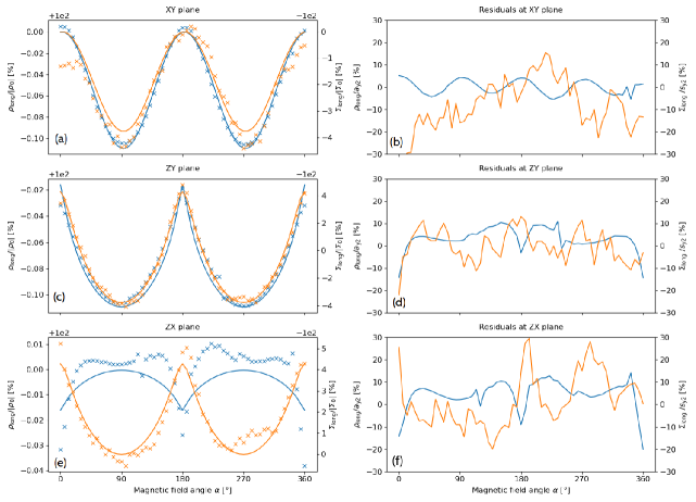
The phenomenological fit to AMR data (blue crosses in Fig. 2) takes into account the uniaxial magnetic anisotropy $k_{\mathrm{u}}$, lowest-order terms $a_{\mathrm{y2}}$ and $a_{\mathrm{z2}}$ and also higher-order AMR terms $a_{\mathrm{y4}}$, $a_{\mathrm{z4}}$ and $a_{\mathrm{zy2}}$. Eq. (4) combined with $k_{u}$ of the SW model resulted in a very good agreement between the data and model. On the other hand, fits omitting the higher-order crystalline terms (specifically, $a_{\mathrm{y4}}$, $a_{\mathrm{z4}}$ and $a_{\mathrm{zy2}}$) shown on the left of Fig. 3 lead to a clear trace of the omitted terms in the residuals. Such a reduced form of Eq. (4) does not allow to reproduce the data well, even when a cubic magnetization anisotropy is included in the SW model (not shown in Fig. 3). The obtained AMR parameters corresponding to $T=300$ K (RT) are shown in Tab. 1.

Figure 2: Results of the AMR and AMTP measurement (crosses) and fitting (continuous lines) in the 50 nm sample at 300 K (AMR) and 250 K (AMTP). a) b), c) Schematic sketch of the magnetic field rotation in the XY, ZY, ZX plane with respect to the coordinate system and the sample. d), e), f) AMR (blue, left y-axes) and AMTP (orange, right y-axes) results; note the shifts of vertical axes indicated at the top of each panel: minimum resistivity, which occurs for $\textbf{m}\parallel\textbf{j}$, is 171 $\mu\Omega$.cm.

AMR Quantity	40 nm	50 nm	40 nm	50 nm	AMTP Quantity
$\rho_{0}$ [$\mu\Omega$ cm]	185.2	186.0	-15.57	-6.61	$\Sigma_{0}$ [$\mu$V/K]
$a_{\mathrm{y2}}$ [$\mu\Omega$ cm]	-0.730	-0.267	-0.216	-0.248	$s_{\mathrm{y2}}$ [$\mu$V/K]
$a_{\mathrm{z2}}$ [$\mu\Omega$ cm]	-0.229	0.046	0.270	0.283	$s_{\mathrm{z2}}$ [$\mu$V/K]
$a_{\mathrm{y4}}$ [$\mu\Omega$ cm]	0.155	0.064	-	-	$s_{\mathrm{y4}}$ [$\mu$V/K]
$a_{\mathrm{z4}}$ [$\mu\Omega$ cm]	-0.242	-0.106	-	-	$s_{\mathrm{z4}}$ [$\mu$V/K]
$a_{\mathrm{zy2}}$ [$\mu\Omega$ cm]	0.008	0.008	-	-	$s_{\mathrm{zy2}}$ [$\mu$V/K]

Table 1: Fitted AMR and AMTP parameters at room temperature.

Figure 3: (a,c,e) Data from Fig. 2 where AMR (AMTP) is fitted by Eq. 4 (Eq. 5, respectively) with second-order terms only; a lower quality, compared to Fig. 2(f), of the AMR fit in the bottom panel is clearly apparent but systematic deviations can also be observed for the XY and ZY rotations. (b,d,f) The difference of the experimental data and fits on the left (fit residuals), see text for a detailed discussion.

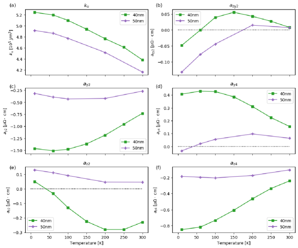
Inferred RT values of $k_{u}$ (438 and 416 kJ/m³ for the 40 and 50 nm sample, respectively) are in a good agreement with ferromagnetic resonance measurements carried out independently Swekis:2020_a and the temperature dependence of such magnetic anisotropy, see Fig. 4(a), is consistent Zener:1954_a with that of the magnetisation (see Fig. 1b). Turning our attention to the transport coefficients, the largest of the AMR parameters is the in-plane lowest-order one: $a_{\mathrm{y2}}$. It is negative, which reflects that the resistivity is smaller for $\textbf{m}\parallel\textbf{j}$ than for $\textbf{m}\perp\textbf{j}$, a situation commonly referred to as negative AMR Tsunoda:2010_a . This is opposite to what is found in more common ferromagnets such as iron, nickel, cobalt and their alloys Turek:2012_a and more importantly, it is also consistent with the finding of Sato et al. Sato:2019 who found a negative AMR ratio $(\rho_{\parallel}-\rho_{\perp})/\rho_{\perp}$ in Co2MnGa for current along [1 1 0]. Some other ferromagnetic systems, (Ga,Mn)As for instance Rushforth:2007_a , carry negative AMR too.

Temperature dependences of the AMR parameters are shown in Fig. 4. Their trends for the 50 nm sample are similar to those of the 40 nm sample except for the out-of-plane lowest-order $a_{\mathrm{z2}}$ parameter; even so, the both data sets in Fig. 4(e) seem to have a minimum slightly below RT. According to the absolute value, the magnitude of the parameters in descending order are as follows: $|a_{\mathrm{y2}}|>|a_{\mathrm{z4}}|>|a_{\mathrm{z2}}|>|a_{\mathrm{y4}}|>|a_{\mathrm{zy2}}|$.

Such observations, however, lack any universal validity. Trends regarding the order of magnitude or the sign of the coefficients can be observed, yet they cannot be generalized. This is also confirmed by results of similar studies in Co2FeAl Althammer:2012 and in (Ga, Mn)As Limmer:2006_a ; Limmer:2008_a ; Althammer:2012 . Hence, there are always exceptions to a rule: $|a_{\mathrm{y2}}|$ is usually the largest of the AMR coefficients (but not for very thin samples Ritzinger:2020_a ) and $a_{\mathrm{y4}}$ is in most cases positive (but not at very low temperatures in the 50 nm sample) to give two examples. Since our model is phenomenological and the microscopic origins of the AMR mechanisms are not fully understood for Co2MnGa, an explanation of the observed behaviour remains an open question.

Attempts to identify the underlying mechanisms of AMR in related materials have been undertaken by Kokado and Tsunoda unknownREF whereas the focus was on electron scattering. They used a two-current model, taking into account $s$-to-$s$ and $s$-to-$d$ scattering. The Hamiltonian of the localized d-states includes spin-orbit interaction, an exchange field and a crystal field of cubic or tetragonal symmetry, where the tetragonal distortion is in [0 0 1] direction. They found that the $a_{\mathrm{y4}}$ contribution ($C_{4}$ in their notation) appears under a tetragonal symmetric crystal field, but almost vanishes under cubic symmetry. This is consistent to other studies that reported that a four-fold-contribution ($a_{\mathrm{y4}}$ in our notation) is not needed to describe the in-plane AMR. However, thin-films are expected to be strained by the substrate and thus to show some tetragonality, which leads to a non-zero $a_{y4}$ contribution. On the other hand, the strain is different in each sample. Thus, studies that reported a two-fold in-plane AMR (i.e. $a_{y4}=0$) might have samples with relatively low strain, which are almost cubic.

Figure 4: Temperature evolution of the parameters obtained by the phenomenological fit to AMR data. (A) Uniaxial magnetic anisotropy, (B-F) parameters for AMR defined in Eq. 4.

AMTP

To fit the AMTP data, we used a procedure analogous to fitting AMR except for the anisotropy constant $k_{\mathrm{u}}$: this parameter has already been determined before and we now kept it fixed. Note, that due to the on-chip heating the actual temperature might be slightly different than indicated. However since the change of $k_{\mathrm{u}}$ with temperature is small, it does not change the accuracy of our approach. Given our measurement geometry, $m_{x}m_{y}m_{z}=0$ at all times, hence Eq. (5) contains the same terms as Eq. (4) and in particular, we started with the lowest-order terms $s_{\mathrm{y2}}$ and $s_{\mathrm{z2}}$. Only these lowest-order parameters and the magnetic anisotropy were needed to obtain good fits to the AMTP data, which is a pronounced difference to the AMR. A reason for this difference could be the noise which is stronger in the AMTP data as compared to the AMR. We have not been able to achieve as good resolution as in the case of the AMR. However, the noise allows us to determine a maximum value of possible higher-order terms, which need to be smaller than the noise. In absolute terms, the noise is of the order of magnitude 0.10 $\mu$V/K and below, which implies that the higher-order symmetries are smaller than about one fifth of the lowest-order symmetries (see Tab. 1). This is not only a striking difference to AMR in our samples, where lower- and higher-order coefficients are in the same order of magnitude, but also to the analysis of AMTP in (Ga,Mn)As by Althammer Althammer:2012 , where the existence of higher-order AMTP parameter is reported. In relative terms, the noise shown in Fig. 3 (as residuals after subtracting the fits from experimental data) is large which is a consequence of difficulties in controlling the temperature gradient under experimental conditions. The temperature evolution of the AMTP parameters as well as a comparison to the lowest-order AMR parameters is shown in Fig. 5(b).

In Fig. 5(a), the Seebeck coefficient $\Sigma_{0}$ is shown as function of temperature. In literature, the Seebeck coefficient of Co2MnGa ranges between approximately $-2\mu$V/K and $-30\mu$V/K at RT, whereas no clear trend is recognizable and the present measurements fall within this range: we find $\Sigma_{0}$ for both samples close to $-15\mu$V/K. Seebeck coefficient of the 50 nm sample is increasing in absolute value with increasing temperature, as expected from previously published experiments Guin2019 ; Balke:2010_a .

Figure 5: a) Longitudinal Seebeck coefficient $\Sigma_{0}$ as a function of the temperature. The different samples are distinguished by the shape of symbols. The absolute value of the Seebeck coefficient of the 50 nm sample is monotonously increasing with temperature. There is a sign change at low temperatures. The Seebeck coefficients at $T=300$ K for the 40 and 50 nm sample are of comparable magnitude. b) Comparison of the AMTP and the corresponding AMR parameters in the 50 nm sample as a function of temperature. AMR and AMTP are distinguished by linestyle. The $m_{\mathrm{y}}^{2}$ contributions are in shades of orange, the $m_{\mathrm{z}}^{2}$ contributions in shades of green. They do not seem to follow any common trend. Error bars of AMTP and AMR parameters in b) (implied by the fitting procedure) are too small to be visually resolved.

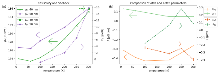
As mentioned in Sec. I, the sign of $\Sigma_{0}$ is attributed to the dominant charge carrier type, which are electrons for $\Sigma_{0}<0$. A negative Seebeck coefficient is reported not only in Co2MnGa, but in Co-based Heusler compounds in general Hu:2020_a . The sign change of $\Sigma_{0}$ would mean that the dominant charge carrier type switches from electrons to holes for decreasing temperatures. This was shown to occur in other materials depending on the doping Lue:2002_a . However, other scenarios are also plausible which we discuss in the next subsection and we now turn our attention to the AMTP.

We notice that neither $s_{\mathrm{y2}}$ nor $s_{\mathrm{z2}}$, whose temperature dependence is shown in Fig. 5(b), can be correlated to their AMR counterparts. While $a_{\mathrm{z2}}$ is decreasing with increasing temperature and the dependence of $a_{\mathrm{y2}}$ is non-monotonic, the AMTP parameters exhibit very different dependence, although they were measured on exactly same device in the and same structure. At $T=250$ K in both AMTP parameters, there is an outlier. This might be due to a thermal offset variation. Together with the sign change of $s_{\mathrm{z2}}$ the lack of correlation between the AMR and AMTP is evident. This is in striking contrast to the transversal transport measured in the same material Park2020 . In that study the AHE and ANE were measured simultaneously and clear correlation was observed including the presence of outliers.

From our study it appears that comparing the lowest-order parameters, no common trend can be found between the AMR parameters and their respective AMTP counterpart when looking at the temperature dependence. Moreover, in case of the ZX rotation (see Fig. 2f), even the raw angular sweep data are clearly very different: the fourth-order terms can be basically seen by naked eye in the AMR while in the AMTP, they are apparently absent and no such terms can be the identified in the residuals on right panels of Fig. 3. In the systematic study of AMR and AMTP in (Ga, Mn) As by Althammer, higher-order contributions have been found for both effects, but the parameters did not appear to be correlated with each other. Since the amount of data in this and all past studies is relatively small, further studies are desirable to investigate if any correlation between AMR und AMTP coefficients exists.

The fact, that in two different systems the AMR and the AMTP follow different trends is, however, a strong indication, that there might be a more fundamental reason behind this discrepancy such as the suppressed role of anisotropic scattering in the AMTP, which calls for further investigation; below, we discuss one possible direction of such tentative research.

Mott rule and phonon drag

Electron and heat transport linear response coefficients are tensorial quantities which obey Onsager relations Smrcka:1976_a and combine into the Seebeck coefficient $\Sigma_{0}$. To see this, we rewrite the electron transport equation as

$$\textbf{E}=\rho\textbf{j}+\Sigma_{0}\nabla T$$

and set $\textbf{j}=0$. Under the assumption of elastic scattering, the Mott rule holds (still in tensorial sense)

$$\Sigma_{0}=-eL_{0}T\rho\sigma^{\prime}=eL_{0}T\rho^{\prime}\sigma$$ (6)

where $\rho\sigma=1$ and the prime denotes the derivative with respect to energy $E$ at chemical potential. For semiconductors, this derivative can be straightforwardly accessed through carrier-density-dependent conductivity Miyasato:2007_a but no such possibility is obvious in our metallic system. However, when resistivity is broken down into a magnetisation-independent background $\rho_{0}$ and a small correction $\Delta\rho$ that effectively constitutes the AMR, the following observation is possible.

Let us first assume that $\rho$ which depends both on $E$ and M can be written as

$$\rho(E,\textbf{M})=\rho_{0}(E)+\Delta\rho(\textbf{M}).$$ (7)

Eq. (6) can then be rewritten as $\Sigma_{0}=eL_{0}T\rho_{0}^{\prime}\sigma$ and since $\rho_{0}$ is a scalar quantity, it essentially implies that AMTP is proportional to the AMR (tensors $\Sigma_{0}$ and $\sigma$ are proportional through a scalar factor). In terms of data shown in Fig. 2, this could seem to imply that dominant non-crystalline contributions of AMR (XY and ZY rotations) indeed follow while the more delicate and smaller crystalline terms (ZX rotation) break the assumption (7) and give different AMR and AMTP angular dependences.

On a careful inspection however, we notice that AMR and AMTP amplitudes in the left and middle panels of Fig. 2 are not proportional the same way as the average $\rho$ and $\Sigma_{0}$ (this is made explicit by scaling of the vertical axes on the left three panels in Fig. 3). While the assumption (7) may be not accurately fulfilled (specifically, the $\Delta\rho$ term is unlikely to be perfectly energy-independent), there is also another possibility to explain this discrepancy. We note that thermopower is strongly temperature-dependent (data in Fig. 5a show that it changes almost by a factor of three between 250 and 300 K) and at the same time, $\rho_{0}$ changes only at the order of per cent in the same temperature interval.

This explanation is related to the phonon drag contribution to thermopower which is not included in the Mott formula (6). In semiconductors, this contribution can easily exceed (see Fig. 12 in Protik&Broido Protik:2020_a ) the electronic thermopower or, in other words, it can reach the level of 100 $\mu$V/K. It is therefore plausible that the measured (relatively small) value of $\Sigma_{0}$ is the result of competition of two (large, relative to $\Sigma_{0}$) contributions: the usual electronic contribution related to the Fermi-Dirac factor $f_{FD}(E)$ depending on temperature and the phonon drag contribution caused by electron-phonon interaction. Once the phonon drag contribution would be removed from the measured $\Sigma_{0}$, the amplitude-to-average ratio of AMTP drops to the same level as for the AMR (here, we again refer to the Fig. 2(b and (d) consistent with proportionality of AMR and AMTP implied by the Mott formula under assumption (7). This way, our measurements suggest a sizable phonon drag effect in the thermopower of Co2MnGa. Alternatively, magnon drag could be at works Watzman:2016_a ; Polash:2020_a . Regarding Fig. 2(f) we note that quite clearly, proportionality between AMR and AMTP is by no means exact and it seems (in the view of data in Fig. 5(b) that thermopower in Co2MnGa is more sensitive to crystallographic orientation than resistivity.

V. SUMMARY

In this study, we compared the AMR and AMTP in two Co2MnGa-thin-film samples using a simple Free Energy density and phenomenological symmetry-based models for AMR and AMTP based on a series expansion in powers of the magnetization direction vector m. We showed that non-zero resistivity-contributions up to 4th order are necessary for a sensible modeling, where in the AMTP only lowest-order contributions are necessary. The AMR and AMTP are not showing any trends in common, which is consistent with previous studies in (Ga, Mn)As. We experimentally confirm presence of a crystalline contribution to the AMTP. It appears that the universal Mott rule validity is broken due to a discrepancy of the symmetries of AMR and AMTP in one rotation plane. This discrepancy was discussed in terms of a significant phonon (magnon) drag contribution to thermopower, which might be the origin of such a discrepancy.

The results of this study call for further enquiry: First of all, we need to broaden our understanding about the origins and governing influences in AMR, but also in AMTP. Theoretical studies discussing influences in AMTP similar to whose about AMR are desirable. Experimental studies using sets of samples which are systematic with respect to strain, composition or other influences can help us also along this way.

Appendix A Notes on derivation of Eqs. 4,5

Comments on the full form of $\rho^{(i)}$ in Eq. (2) are given here, from which Eq. (4) can be derived. A more detailed description can be found in Appendix A.1 of thesis Ritzinger:2020_a of one of the authors. Only terms corresponding to cubic symmetry are included and summation over repeated indexes (Einstein notation) is implied. Note that the underlying coordinate system is equivalent to the one applied in Eq. 2, thus: $m_{\mathrm{n}}\in\{m_{\hkl[100]},m_{\hkl[010]},m_{\hkl[001]}\}$. We skip $\rho_{\mathrm{ijk}}^{(1)}$ which does not appear in $\rho_{\mathrm{long}}$ the in-plane geometry (it corresponds to the anomalous Hall effect). The lowest non-trivial order thus becomes

$$\rho_{\mathrm{ijkl}}^{(2)}m_{\mathrm{k}}m_{\mathrm{l}}=C_{1}\left(\begin{array}[]{ccc}m_{\mathrm{x}}^{2}&0&0\\ 0&m_{\mathrm{y}}^{2}&0\\ 0&0&m_{\mathrm{z}}^{2}\end{array}\right)+C_{2}\left(\begin{array}[]{ccc}0&m_{\mathrm{x}}m_{\mathrm{y}}&m_{\mathrm{x}}m_{\mathrm{z}}\\ m_{\mathrm{x}}m_{\mathrm{y}}&0&m_{\mathrm{y}}m_{\mathrm{z}}\\ m_{\mathrm{x}}m_{\mathrm{z}}&m_{\mathrm{y}}m_{\mathrm{z}}&0\end{array}\right).$$

The third-order terms, $\rho_{\mathrm{ijklm}}^{(3)}$, again do not contribute in Eq. (3), and the fourth-order terms $\rho_{\mathrm{ijklmn}}^{(4)}m_{\mathrm{k}}m_{\mathrm{l}}m_{\mathrm{m}}m_{\mathrm{n}}$ become

$$E_{1}\left(\begin{array}[]{ccc}m_{\mathrm{x}}^{4}&0&0\\ 0&m_{\mathrm{y}}^{4}&0\\ 0&0&m_{\mathrm{z}}^{4}\end{array}\right)+E_{2}\left(\begin{array}[]{ccc}m_{\mathrm{y}}^{2}m_{\mathrm{z}}^{2}&0&0\\ 0&m_{\mathrm{x}}^{2}m_{\mathrm{z}}^{2}&0\\ 0&0&m_{\mathrm{x}}^{2}m_{\mathrm{y}}^{2}\end{array}\right)+E_{3}\left(\begin{array}[]{ccc}0&m_{\mathrm{x}}m_{\mathrm{y}}m_{\mathrm{z}}^{2}&m_{\mathrm{x}}m_{\mathrm{z}}m_{\mathrm{y}}^{2}\\ m_{\mathrm{x}}m_{\mathrm{y}}m_{\mathrm{z}}^{2}&0&m_{\mathrm{y}}m_{\mathrm{z}}m_{\mathrm{x}}^{2}\\ m_{\mathrm{x}}m_{\mathrm{z}}m_{\mathrm{y}}^{2}&m_{\mathrm{y}}m_{\mathrm{z}}m_{\mathrm{x}}^{2}&0\end{array}\right).$$

Additional terms appear when lower symmetry is assumed, which is in our case due to the tetragonal distortion along the $\hat{z}=\hkl[001]$ axis of the thin-film samples. The following zeroth-order and second-order terms add to the resistivity tensor in the case of tetragonal symmetry:

$$\left(\begin{array}[]{rrr}0&0&0\\ 0&0&0\\ 0&0&a\\ \end{array}\right)+\left(\begin{array}[]{ccc}c_{3}m_{\mathrm{z}}^{2}&0&c_{2}m_{\mathrm{x}}m_{\mathrm{z}}\\ 0&c_{3}m_{\mathrm{z}}^{2}&c_{2}m_{\mathrm{y}}m_{\mathrm{z}}\\ c_{2}m_{\mathrm{x}}m_{\mathrm{z}}&c_{2}m_{\mathrm{y}}m_{\mathrm{z}}&c_{1}m_{\mathrm{z}}^{2}\\ \end{array}\right)$$

Under tetragonal symmetry, the fourth-order terms are supplemented by:

$$\left(\begin{array}[]{ccc}e_{2}m_{\mathrm{y}}^{2}m_{\mathrm{z}}^{2}+e_{4}m_{\mathrm{z}}^{4}&e_{3}m_{\mathrm{x}}m_{\mathrm{y}}m_{\mathrm{z}}^{2}&e_{6}m_{\mathrm{x}}m_{\mathrm{y}}^{2}m_{\mathrm{z}}+e_{7}m_{\mathrm{x}}m_{\mathrm{z}}^{3}\\ e_{3}m_{\mathrm{x}}m_{\mathrm{y}}m_{\mathrm{z}}^{2}&e_{2}m_{\mathrm{x}}^{2}m_{\mathrm{z}}^{2}+e_{4}m_{\mathrm{z}}^{4}&e_{6}m_{\mathrm{x}}^{2}m_{\mathrm{y}}m_{\mathrm{z}}+e_{7}m_{\mathrm{y}}m_{\mathrm{z}}^{3}\\ e_{6}m_{\mathrm{x}}m_{\mathrm{y}}^{2}m_{\mathrm{z}}+e_{7}m_{\mathrm{x}}m_{\mathrm{z}}^{3}&e_{6}m_{\mathrm{x}}^{2}m_{\mathrm{y}}m_{\mathrm{z}}+e_{7}m_{\mathrm{y}}m_{\mathrm{z}}^{3}&e_{5}m_{\mathrm{x}}^{2}m_{\mathrm{y}}^{2}+e_{1}m_{\mathrm{z}}^{4}\\ \end{array}\right)$$

In a similar (yet distinct) manner, the Seebeck tensor can be expanded, see Appendix B.1 of Ref. Ritzinger:2020_a . In the case of tetragonal symmetry, to which Eq. (5) applies, several additional terms appear but they do not contribute to $\Sigma_{\mathrm{yy}}$ except for

$$D_{7}m_{\mathrm{x}}m_{\mathrm{y}}m_{\mathrm{z}}\left(\begin{array}[]{ccc}-1&0&0\\ 0&1&0\\ 0&0&0\end{array}\right)$$

which gives rise to the last term in Eq. (5). Therefore even in our setup, $\rho_{\mathrm{yy}}$ and $\Sigma_{\mathrm{yy}}$ allow in principle for a different functional form albeit not with our constraint to XY, YZ, and XZ rotations of magnetic field. Further information can be found in Ref. Althammer:2012 or in the Appendix of Ref. Ritzinger:2020_a .

References

- (1) W. Thomson, Proc. R. Soc. Lond. 8, 546-550 (1856)
- (2) M. Wang, C. Andrews, S. Reimers, O. J. Amin, P. Wadley, R. P. Campion, S. F. Poole, J. Felton, K. W. Edmonds, B. L. Gallagher, A. W. Rushforth, O. Makarovsky, K. Gas, M. Sawicki, D. Kriegner, J. Zubáč, K. Olejník, V. Novák, T. Jungwirth, M. Shahrokhvand, U. Zeitler, S. S. Dhesi, and F. Maccherozzi, Phys. Rev. B 101, 094429 (2020)
- (3) J. Volný, D. Wagenknecht, J. Železný, P. Harcuba, E. Duverger–Nedellec, R. H. Colman, J. Kudrnovský, I. Turek, K. Uhlířová, and K. Výborný, Phys. Rev. Materials 4, 064403 (2020).
- (4) Y. Miao, X. Chen and D.–S. Xue, J. Magn. Magn. Mat. 512, 167013 (2020).
- (5) D. Wesenberg, A. Hojem, R. K. Bennet and B. L. Zink, J. Phys. D: Appl. Phys. 51 244005 (2018)
- (6) H. Yu, S. D. Brechet, J.-P. Ansermet, Phys. Lett. A 381, 825-837 (2017)
- (7) Fig. 8 and Tab. 2 in J. Hu, S. Granville, H. Yu, Ann. Phys., Lpz. 532, 1900456 (2020)
- (8) A. Sakai, Y. P. Mizuta, A. A. Nugroho, R. Sihombing, T. Koretsune, M.-T. Suzuki, N. Takemori, R. Ishii, D. Nishio-Hamane, R. Arita, P. Goswami and S. Nakatsuji, Nat. Phys. 14, 1119–1124 (2018)
- (9) H. Reichlova, R. Schlitz, S. Beckert, P. Swekis, A. Markou, Y.-C. Chen, D. Kriegner, S. Fabretti, G. H. Park, A. Niemann, S. Sudheendra, A. Thomas, K. Nielsch, C. Felser, and S. T. B. Goennenwein, Appl. Phys. Lett. 113, 212405 (2018)
- (10) I. Belopolski, K. Manna, D. S. Sanchez, G. Chang, B. Ernst, J. Yin, S. S. Zhang, T. Cochran, N. Shumiya, H. Zheng, B. Singh, G. Bian, D. Multer, M. Litskevich, X. Zhou, S.-M. Huang, B. Wang, T.-R. Chang, S.-Y. Xu, A. Bansil, C. Felser, H. Lin, and M. Z. Hasan, Science 365, 1278 (2019).
- (11) G.-H. Park, H. Reichlova, R. Schlitz, M. Lammel, A. Markou, P. Swekis, P. Ritzinger, D. Kriegner, J. Noky, J. Gayles, Y. Sun, C. Felser, K. Nielsch, S. T. B. Goennenwein, and A. Thomas, Phys. Rev. B 101 (2020)
- (12) T. Graf, C. Felser, S. S. P. Parkin, Prog. Solid. State Ch. 39, 1-50 (2011)
- (13) N. H. Protik and D. A. Broido, Phys. Rev. B 101, 075202 (2020)
- (14) Md. M. H. Polash, F. Mohaddes, M. Rasoulianboroujeni, D. Vashaee, J. Mater. Chem. C 8, 4049-4057 (2020)
- (15) A. W. Rushforth, K. Výborný, C. S. King, K. W. Edmonds, R. P. Campion, C. T. Foxon, J. Wunderlich, A. C. Irvine, P. Vašek, V. Novák, K. Olejník, Jairo Sinova, T. Jungwirth, and B. L. Gallagher, Phys. Rev. Lett. 99, 147207 (2007)
- (16) W. Döring, Ann. Phys., Lpz. 424, 259 (1938)
- (17) E. De Ranieri, A. W. Rushforth, K. Výborný, U. Rana, E. Ahmad, R. P. Campion, C. T. Foxon, B. L. Gallagher, A. C. Irvine, J. Wunderlich, New J. Phys. 10, 065003 (2008)
- (18) V. D. Ky, Phys. Status Solidi B 17, K207 (1966).
- (19) G. J. Snyder and E. S. Toberer, Nat. Mater. 7, 105–114 (2008)
- (20) T. Janda, J. Godinho, T. Ostatnicky, E. Pfitzner, G. Ulrich, A. Hoehl, S. Reimers, Z. Šobáň, T. Metzger, H. Reichlová, V. Novák, R. P. Campion, J. Heberle, P. Wadley, K. W. Edmonds, O. J. Amin, J. S. Chauhan, S. S. Dhesi, F. Maccherozzi, R. M. Otxoa, P. E. Roy, K. Olejník, P. Nemec, T. Jungwirth, B. Kaestner, and J. Wunderlich, Phys. Rev. Materials 4, 094413 (2020)
- (21) O.M.Løvvik, Espen Flage-Larsen, and Gunstein Skomedal, J. Appl. Phys. 128, 125105 (2020)
- (22) Electronic bands in the bulk can be characterised by topological invariants which indicate whether or not there will be surface states. These are related to Berry curvature, a quantity related to ANE Sakai2018 , through Eq. 2 of J. Kübler and C. Felser, Europhys. Lett. 114, 47005 (2016).
- (23) A. Sakai, S. Minami, T. Koretsune, T. Chen, T. Higo, Y. Wang, T. Nomoto, M. Hirayama, S. Miwa, D. Nishio-Hamane, F. Ishii, R. Arita and S. Nakatsuji, Nature 581, 53 (2020)
- (24) W. Limmer, J. Daeubler, L. Dreher, M. Glunk, W. Schoch, S. Schwaiger, and R. Sauer, Phys. Rev. B 77, 205210 (2008).
- (25) M. Althammer, doctoral thesis, Technische Universität München, 2012
- (26) O. Reimer, D. Meier, M. Bovender, L. Helmich, J.-O. Dreessen, J. Krieft, A. S. Shestakov, C. H. Back, J.-M. Schmalhorst, A. Hütten, G. Reiss and T. Kuschel, Sci. Rep. 7, 40586 (2017)
- (27) P.B.Jayathilaka, D.D.Belyea, T.J.Fawcett, and Casey W.Miller, J. Magn. Magn. Mat. 382, 376 (2015).
- (28) T. Janda, J. Godinho, T. Ostatnicky, E. Pfitzner, G. Ulrich, A. Hoehl, S. Reimers, Z. Šobán, T. Metzger, H. Reichlová, V. Novák, R. P. Campion, J. Heberle, P. Wadley, K. W. Edmonds, O. J. Amin, J. S. Chauhan, S. S. Dhesi, F. Maccherozzi, R. M. Otxoa, P. E. Roy, K. Olejník, P. Nemec, T. Jungwirth, B. Kaestner, and J. Wunderlich, Phys. Rev. Materials 4, 094413 (2020)
- (29) A. D. Avery, M. R. Pufall, and B. L. Zink, Phys. Rev. Lett. 109, 196602 (2012)
- (30) A. Markou, D. Kriegner, J. Gayles, L. Zhang, Y.-C. Chen, B. Ernst, Y.-H. Lai, W. Schnelle, Y.-H. Chu, Y. Sun, and C. Felser, Phys. Rev. B 100, 054422 (2019)
- (31) U. Pietsch, V. Holý, and T. Baumbach, High-resolution X-ray Scattering: From Thin Films to Lateral Nanostructures (Springer, New York, 2004).
- (32) W. Limmer, M. Glunk, J. Daeubler, T. Hummel, W. Schoch, R. Sauer, C. Bihler, H. Huebl, M. S. Brandt, and S. T. B. Goennenwein, Phys. Rev. B 74, 205205 (2006)
- (33) E. C. Stoner and E. P. Wohlfarth, Phil. Trans. Roy. Soc. A 240, 599 (1948).
- (34) P. Swekis, A. S. Sukhanov, Y.-C. Chen, A. Gloskovskii, G. H. Fecher, I. Panagiotopoulos, V. Ukleev, A. Devishvili, A. Vorobiev, D. S. Inosov, S. T. B. Goennenwein, C. Felser and A. Markou (unpublished)
- (35) A tensor representing a macroscopic physical property of a crystal must be invariant under all symmetry operations of the corresponding point-group.
- (36) C. Zener, Phys. Rev. 96, 1335 (1954).
- (37) M. Tsunoda, H. Takahashi, S. Kokado, Y. Komasaki, A. Sakuma and M. Takahashi, Appl. Phys. Express 3, 113003 (2010)
- (38) I. Turek, J. Kudrnovský, and V. Drchal, Phys. Rev. B 86, 014405 (2012).
- (39) T. Sato, S. Kokado, M. Tsujikawa, T. Ogawa, S. Kosaka, M. Shirai and M. Tsunoda, Appl. Phys. Express 12, 103005 (2019)
- (40) P. Ritzinger, master thesis, Technische Universität Dresden, 2020
- (41) S. Kokado and M. Tsunoda, J. Phys. Soc. Jpn. 84, 094710 (2015).
- (42) S. N. Guin, K. Manna, J. Noky, S. J. Watzman, C. Fu, N. Kumar, W. Schnelle, C. Shekhar, Y. Sun, J. Gooth, and C. Felser, NPG Asia Mater. 11:16 (2019)
- (43) B. Balke, S. Ouardia, T. Graf, J. Barth, C. G. F. Blum, G. H. Fecher, A. Shkabko, A. Weidenkaff, C. Felser, Sol. St. Comm. 150, 529 (2010).
- (44) C. S. Lue and Y.-K. Kuo, Phys. Rev. B 66, 085121 (2002).
- (45) L. Smrčka and P. Vašek, Czech. J. Phys. B 26, 1137–1147 (1976)
- (46) T. Miyasato, N. Abe, T. Fujii, A. Asamitsu, S. Onoda, Y. Onose, N. Nagaosa, and Y. Tokura, Phys. Rev. Lett. 99, 086602 (2007)
- (47) S. J. Watzman, R. A. Duine, Y. Tserkovnyak, S. R. Boona, H. Jin, A. Prakash, Y. Zheng, and J. P. Heremans, Phys. Rev. B 94, 144407 (2016)