Causal World Models by Unsupervised Deconfounding of Physical Dynamics

Abstract

The capability of imagining internally with a mental model of the world is vitally important for human cognition. If a machine intelligent agent can learn a world model to create a "dream" environment, it can then internally ask what-if questions – simulate the alternative futures that haven’t been experienced in the past yet – and make optimal decisions accordingly. Existing world models are established typically by learning spatio-temporal regularities embedded from the past sensory signal without taking into account confounding factors that influence state transition dynamics. As such, they fail to answer the critical counterfactual questions about "what would have happened" if a certain action policy was taken. In this paper, we propose Causal World Models (CWMs) that allow unsupervised modeling of relationships between the intervened observations and the alternative futures by learning an estimator of the latent confounding factors. We empirically evaluate our method and demonstrate its effectiveness in a variety of physical reasoning environments. Specifically, we show reductions in sample complexity for reinforcement learning tasks and improvements in counterfactual physical reasoning.

1 Introduction

Human-level intelligence relies on building up the capability of simulating the physical world in order to create human-like thinking, reasoning, and decision making abilities (Lake et al., 2015, 2017; Spelke & Kinzler, 2007). This mechanism has served as a core motivation behind several recent works of learning world models (WMs) that aim at predicting future sensory data given the agent’s current motor actions (Greff et al., 2017; Kipf et al., 2020; van Steenkiste et al., 2018; Xu et al., 2019). One of the ultimate goals of WMs is creating the dream, where the agent can internally simulate the alternative futures not encountered in the real world (Ha & Schmidhuber, 2018). This, however, requires WMs to predict the reasonable outcome of various types of interventions to the observation. In this paper, we explore building WMs capable of creating the dream environment to predict the counterfacts that would have happened.

Conventional world models usually aim at learning spatio-temporal regularities from the past data and thereby predict future frames from one or several past frame(s). These models typically employ standard IID function learning techniques without considering the causal effect of the interventions (Balke & Pearl, 1995). However, as an agent interacts with the environment and thus influences the statistics of the gathered data over time, the IID assumption is violated (Schölkopf, 2019). By looking for invariances from observational data has been shown to help identify robust components and causal features of the environment (Peters et al., 2017). For example in the physical dynamics systems, these features could be the underneath confounding factors (or confounders) affecting the environment across temporality such as inertia, velocity, gravity or friction. Accurate estimation of these factors enables model-based RL agents to generalize to other parts of the state space and thus being more robust. Correcting for the confounding effect could also influence the policy to be optimized (Lu et al., 2018).

In this paper, we introduce the Causal World Models (CWMs) to predict the effect of interventions that would have happened, i.e., we wish to predict consequent observation trajectories if we had changed the initial observation by performing an external intervention, which is defined as an object-level observable change applied to the initial observation. CWMs aim at modeling relationships between the variable on which the intervention is performed and the variable whose alternative future should be predicted. Our model starts from learning a set of abstract state variables for each object in a particular observation and model the transition using graph neural networks (Battaglia et al., 2018; Kipf & Welling, 2017; Li et al., 2016; Scarselli et al., 2009) that operate on latent abstract representations. We then develop CWMs by estimating the latent representation of the confounders, i.e., a set of static but visually unobservable quantities that could otherwise affect the observation. In our method, the deconfounding process could be understood as an extension on conventional World Models. Deconfounding methods help to build time-invariant function beyond transition functions, which gives a more precise description of the environment by preserving global information, such as gravity acceleration in physical systems, from time variations. The alternative future is then predicted given the altered past and the estimation of confounders. To further reduce the intrinsic bias owing to the inadequate counterfactual records, we also propose a counterfactual risk minimization method from historical observations for CWMs. We empirically evaluate our method and demonstrate its effectiveness in CoPhy (Baradel et al., 2020) (a counterfactual physics benchmark suite) and PHYRE (Bakhtin et al., 2019) (a physical reasoning benchmark with reinforcement learning tasks). Specifically, we show reductions in sample complexity for reinforcement learning and improvements in counterfactual physical reasoning.

2 Related Work

The task in observational discovery of causal effects in physical reality is usually concerned with predicting the effect of various types of interventions, including physical laws underneath the environment (Battaglia et al., 2016; Chang et al., 2017; Wu et al., 2015), the actions executed by the agent itself (Levine & Abbeel, 2014; Li et al., 2019; Wahlström et al., 2015; Watter et al., 2015), and the outcome of other agents’ decision in multi-agent systems (He et al., 2016; Tian et al., 2019). While causal reasoning has gained mainstream attention in the machine learning field recently (Lopez-Paz & Oquab, 2017; Mooij et al., 2016; Schölkopf, 2019), the current literature mostly focuses on discovering the causal effect between variables in static environments (Chalupka et al., 2015; Kocaoglu et al., 2018; Lopez-Paz et al., 2017). Extensive research has also been conducted on visual reasoning in static environments (Eslami et al., 2016; Hudson & Manning, 2018; Johnson et al., 2017; Mao et al., 2019; Santoro et al., 2017). Although Lu et al. (2018) has considered deconfounding in the reinforcement learning scenario, their assumption only covers the confounding between the observations, actions and rewards, thus failing to predict counterfactual scenarios by deconfounding the state transitions. By contrast, our proposed CWMs take into account the confounding factors between state transitions and can therefore internally predict the alternative futures not encountered in the past.

Understanding intuitive physics from visual perception has attracted considerable attention in machine learning and reinforcement learning society (Kubricht et al., 2017; Lerer et al., 2016; Wu et al., 2015, 2017; Sun et al., 2018, 2019). Many of the existing models require supervised modeling of the object definition, by either comparing the activation spectrum generated from neural network filters with existing types (Garnelo et al., 2016) or leveraging the bounding boxes generated by standard object detection algorithms in computer vision (Keramati et al., 2018). Although (Zambaldi et al., 2019) have used the relational mechanism to discover and reason about relevant entities, their model needs additional supervision to label entities with location information. On the contrary, CWMs use a fully unsupervised manner to extract object abstractions. To the best of our knowledge, CoPhyNet (Baradel et al., 2020) is the only work considering counterfactual scenario in learning physical dynamics but used direct supervision of the object positions, thus only performing counterfactual forecasting in low-dimensional settings. Nevertheless, we still benefit from their proposed evaluation benchmark and demonstrate the effectiveness of our fully unsupervised causal world models in Section 4.

A variety of object-based World Models (WMs) have been proposed (Greff et al., 2017; van Steenkiste et al., 2018; Watters et al., 2019) thanks to recent works studying the problem of object discovery from visual data (Burgess et al., 2019; Chang et al., 2017; Engelcke et al., 2020; Greff et al., 2019; Janner et al., 2019; Kosiorek et al., 2018; Sun et al., 2018, 2019; Watters et al., 2017; Xu et al., 2019; Zheng et al., 2018). By exploiting WMs’ ability to think and plan ahead (Ha & Schmidhuber, 2018; Zhu et al., 2018), model-based reinforcement learning algorithms have been shown to be more effective than model-free alternatives in certain tasks (Gu et al., 2016; Igl et al., 2018; Watter et al., 2015; Levine et al., 2016). However, these models are often bottlenecked by the credit-assignment problem: they typically optimize a prediction or reconstruction objective function in pixel space and thereby could ignore visually small but informative features for predicting the future (such as, for instance, a bullet in an Atari game (Łukasz Kaiser et al., 2020)). On the contrary, CWMs learn a set of object-centric abstract state variables and model the transition using graph neural networks (Battaglia et al., 2016, 2018; Kipf et al., 2018; Kipf & Welling, 2017; Li et al., 2016; Scarselli et al., 2009; Wang et al., 2018; Sanchez-Gonzalez et al., 2018) by optimizing an energy-based hinge loss (LeCun et al., 2006) in the latent space directly.

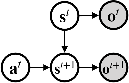
(a)

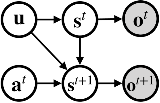
(b)

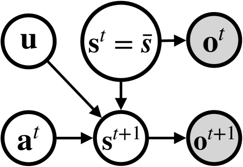
(c)

Figure 1: The graphical model of (a) POMDPs used by conventional WMs, (b) causal POMDPs used by CWMs, and (c) CWMs after intervention (do-operation).

Our proposed model adopts counterfactual learning to mitigate the problem of biased historical data. Counterfactual Risk Minimization (CRM) (Swaminathan & Joachims, 2015b, c) is an instance of causal inference closely related to off-policy evaluation (Kallus & Zhou, 2018). Because the distribution of factual and counterfactual are not fully consistent, causal models built upon historical data will produce bias. Existing work has therefore considered unbiased learning by inverse propensity scores (IPS) methods (Rosenbaum & Rubin, 1983). Most existing literature focuses on the scenarios of binary or limited discrete interventions (Athey & Wager, 2017), including the popular doubly robust frameworks  (Cassel et al., 1976; Dudík et al., 2011; Robins et al., 1994). Instead of measuring the causal effect of the intervention in a discrete event space, our work focuses on the intervention distribution in continuous space. In order to solve the problems of zero propensity scores on continuous intervention setting, Kallus & Zhou (2018) used kernel functions to achieve a smooth policy learning process, while Swaminathan & Joachims (2015c) regularized the empirical risk via variance penalization. Further discussion on this topic can be found in (Louizos et al., 2017; Saito & Yasui, 2019; Swaminathan & Joachims, 2015b, d). Staying different from above approaches, the propensity weight in our method is not decided by the environments state, but decided by the historical sampling strategies.

3 Causal World Models

Our goal is to build a world model capable of creating the dream environment by predicting the effect of interventions that would have happened. We start by introducing the notation and the problem definition of causality in learning physical dynamics. Then, we introduce the general framework for learning object-oriented state abstractions and estimating the confounders. Lastly, we introduce the usage of doubly robust functions - a key technique in robust statistics and efficiency theory (Dudík et al., 2011) - to enhance the sample efficiency and reduce the bias induced by the historical sample policy.

3.1 Preliminary: POMDPs

As shown in Figure 1(a), conventional WMs typically consider the environment as a partially observable Markov Decision Process (POMDP) represented by the tuple $\Gamma={\langle}\mathcal{S},\mathcal{A},\mathcal{O},\mathcal{U},\mathcal{T},\mathcal{R},{T}{\rangle}$, where $\mathcal{S},\mathcal{A},\mathcal{O},{T}$ are the state space, the action space, the observation space, and the horizon, respectively. For an agent taking actions in this environment, we consider the variable representing its received observation at time step $t$ be designated by ${\mathbf{o}}^{t}$, the real-world observed values by ${\bm{o}}^{t}\in\mathcal{O}\equiv\mathbb{R}^{D}$. At each time step $t$, we denote as ${\mathbf{s}}^{t}$ the variable representing the abstract state of the world and ${\bm{s}}^{t}\in\mathcal{S}\equiv\mathbb{R}^{d}$ the real-world value of this variable. ${\mathbf{s}}^{t}$ can be typically regarded as the latent static component of the world to render the observation, e.g., the shape, size and color of the objects. The observation ${\bm{o}}^{t}$ are provided by the environment following the observation distribution $\mathcal{U}({\mathbf{o}}^{t}|{\mathbf{s}}^{t}):\mathcal{S}\rightarrow\mathcal{O}$. When the environment receives an action $a^{t}\in\mathcal{A}$ executed by the agent, it moves to a new state ${\bm{s}}^{t+1}$ following the transition distribution $\mathcal{T}({\mathbf{s}}^{t+1}|{\mathbf{s}}^{t},a^{t}):\mathcal{S}\times\mathcal{A}\rightarrow\mathcal{S}$ and returns a reward $r^{t}$ according to $\mathcal{R}(r^{t}|{\mathbf{s}}^{t},a^{t}):\mathcal{S}\times\mathcal{A}\rightarrow\mathbb{R}$. Conventional WMs focus on estimating the distribution of ${\mathbf{s}}^{t+1}$ given the observed value of ${\mathbf{s}}^{t}$ and $a^{t}$ . This estimation will give us the observational conditional $p({\mathbf{s}}^{t+1}|{\mathbf{s}}^{t},a^{t})$. We will see below that the observational conditional is generally biased in the real world where confounding factors widely exist.

3.2 Causal POMDPs

In this paper, we extend the above typical setting of a POMDP by considering the existence of confounding factors ${\mathbf{u}}$ (Balke & Pearl, 1994), which are time-invariant hidden variables that influence both the intervention ${\mathbf{s}}^{t}$ and the outcome ${\mathbf{s}}^{t+1}$ as shown in Figure 1(b). In physical systems, we regard ${\mathbf{u}}$ as a set of static but visually unobservable quantities such as object masses, friction coefficients, direction and magnitude of gravitational forces that cannot be uniquely estimated from a single time step. Building world models upon causal POMDPs enables us to control the state ${\mathbf{s}}^{t}$ to create the dream environment and facilitate imagination. In other words, we intend to know what the scenario ${\mathbf{s}}^{t+1}$ world have been if we set the world state ${\mathbf{s}}^{t}$ to a specific value $\bar{{\bm{s}}}$. We adopt the do-operator $\textbf{do}({\mathbf{s}}^{t}=\bar{{\bm{s}}})$ from causal reasoning (Pearl, 2009), and arrives at the interventional conditional $p({\mathbf{s}}^{t+1}|\textbf{do}({\mathbf{s}}^{t}=\bar{{\bm{s}}}),a^{t})$. In most real-world cases, the observational conditional and the interventional conditional are different because of the existence of confounding factors ${\mathbf{u}}$. To illustrate the impact, we provide simple calculations for the observational conditional

$$p({\mathbf{s}}^{t+1}|{\mathbf{s}}^{t},a^{t}) =\int_{\mathcal{{\mathbf{u}}}}p({\mathbf{s}}^{t+1}|{\mathbf{u}},{\mathbf{s}}^{t},a^{t})p({\mathbf{u}}|{\mathbf{s}}^{t},a^{t})d{\mathbf{u}}$$

$$=\int_{\mathcal{{\mathbf{u}}}}p({\mathbf{s}}^{t+1}|{\mathbf{u}},{\mathbf{s}}^{t},a^{t})\frac{p({\mathbf{s}}^{t},a^{t}|{\mathbf{u}})}{p({\mathbf{s}}^{t},a^{t})}p({\mathbf{u}})d{\mathbf{u}},$$

and the interventional conditional

$$p({\mathbf{s}}^{t+1}|\textbf{do}({\mathbf{s}}^{t}=\bar{{\bm{s}}}),a^{t})=\int_{\mathcal{{\mathbf{u}}}}p({\mathbf{s}}^{t+1}|{\mathbf{u}},{\mathbf{s}}^{t}=\bar{{\bm{s}}},a^{t})p({\mathbf{u}})d{\mathbf{u}}.$$

Clearly the above two are not the same due to the influence of the confounders ${\mathbf{u}}$: $p({\mathbf{s}}^{t},a^{t}|{\mathbf{u}})$. This result is also termed as the Simpson’s paradox (Simpson, 1951), a classical example for the existence of confounding in medical treatment scenario (see Appendix A for details). The above observations therefore encourage us to build the world model following the causal POMDPs in Figure 1(b), which enables the world model to disentangle the true effect of an intervention on the observation (Louizos et al., 2017).

3.3 Learning Causal World Models

To learn the transition function of the dream world, we apply the do-intervention (Pearl, 2009) $\textbf{do}({\mathbf{s}}^{t}=\bar{{\bm{s}}}^{t})$ on the abstract state variable as shown in Figure 1(c), where $\bar{{\bm{s}}}^{t}\in\mathcal{S}\equiv\mathbb{R}^{d}$ is the counterfactual value in the dream environment. The intervened abstract state is then rendered as an object-level observable change applied to ${\bm{o}}^{t}$ (such as, for instance, object displacement or removal) by the conditional observation distribution $\mathcal{U}({\mathbf{o}}^{t}=\bar{{\bm{o}}}^{t}|\textbf{do}({\mathbf{s}}^{t}=\bar{{\bm{s}}}^{t}))$, where $\bar{{\bm{o}}}^{t}\in\mathcal{O}\equiv\mathbb{R}^{D}$ represents the value of the counterfactual observation.

Learning the causal world models aims at answering:

Given that we have observed ${\mathbf{o}}^{t:T}={\bm{o}}^{t:T}$ in the real world, what is the probability that ${\mathbf{o}}^{t+1:T}$ would have been $\bar{{\bm{o}}}^{t+1:T^{\prime}}$ if ${\mathbf{o}}^{t}$ were $\bar{{\bm{o}}}^{t}$ in the dream world?

Particularly, having observed the tuple $({\bm{o}}^{t:T},\bar{{\bm{o}}}^{t})$, we wish to predict positions and poses of all objects in the scene at time $t={T}^{\prime}$. We consider an off-policy setting for the model training, where we operate solely on a buffer of offline experience obtained from, such as, an exploration policy. In this paper, we focus on building an internal dream environment to simulate the future not encountered in the past with any given dream policy $p(a^{t}|{\mathbf{s}}^{t})$. We therefore drop the action variable from the notation in the remainder of this paper by $\int_{a^{t}}\mathcal{T}({\mathbf{s}}^{t+1}|{\mathbf{s}}^{t},a^{t})p(a^{t}|{\mathbf{s}}^{t})da^{t}=\int_{a^{t}}\mathcal{T}({\mathbf{s}}^{t+1},a^{t}|{\mathbf{s}}^{t})da^{t}=\mathcal{T}({\mathbf{s}}^{t+1}|{\mathbf{s}}^{t}).$

Instead of recovering the individual treatment effect (ITE), which measures the causal effect when the intervention happens in a discrete event space (Alaa & van der Schaar, 2019; Louizos et al., 2017; Saito & Yasui, 2019), we focus on the identification of the intervention distributions $p({\mathbf{o}}^{t+1:{T^{\prime}}}|\textbf{do}({\mathbf{s}}^{t}=\bar{{\bm{s}}}^{t}))$ and $p({\mathbf{o}}^{t}|\textbf{do}({\mathbf{s}}^{t}=\bar{{\bm{s}}}^{t}))$ in the continuous space.

Definition 1.

We say a variable ${\mathbf{u}}$ factorizes the distribution of variable ${\mathbf{s}}^{t}$ iff: $p({\mathbf{s}}^{t})=\int_{\mathcal{{\mathbf{u}}}}p\left({\mathbf{s}}^{t}|{\mathbf{u}}={\bm{u}}\right)p({\mathbf{u}}={\bm{u}})d{\mathbf{u}}.$

Assumption 1.

There exists an unobserved variable ${\mathbf{u}}$ such that (i) ${\mathbf{u}}$ blocks all backdoor path from ${\mathbf{s}}^{t}$ to ${\mathbf{s}}^{t+1}$ and (ii) there exist no backdoor path from the abstract state ${\mathbf{s}}^{t}$ to the observation ${\mathbf{o}}^{t}$.

Theorem 1.

Under Assumption 1, if there exists an estimator of ${\mathbf{u}}$, $\hat{{\mathbf{u}}}({\mathbf{s}}^{t})$, such that $\hat{{\mathbf{u}}}({\mathbf{s}}^{t})\stackrel{{\scriptstyle a\cdot s}}{{\longrightarrow}}{\mathbf{u}},$ then the intervention distributions $p({\mathbf{o}}^{t+1:{T^{\prime}}}|\textbf{do}({\mathbf{s}}^{t}=\bar{{\bm{s}}}^{t}))$ and $p({\mathbf{o}}^{t}|\textbf{do}({\mathbf{s}}^{t}=\bar{{\bm{s}}}^{t}))$ are identifiable.

Proof.

By applying do-calculus to the causal graph in Figure 1(b) (as shown in Figure 1(c)), referred to back-door criterion, the intervention distributions are then identified by

$$p({\mathbf{o}}^{t}|\textbf{do}({\mathbf{s}}^{t}=\bar{{\bm{s}}}^{t}))=p({\mathbf{o}}^{t}|{\mathbf{s}}^{t}=\bar{{\bm{s}}}^{t}),$$

$$p({\mathbf{o}}^{t+1:{T^{\prime}}}|\textbf{do}({\mathbf{s}}^{t}=\bar{{\bm{s}}}^{t}))=\int_{\mathcal{{\mathbf{u}}}}p({\mathbf{o}}^{t+1:{T^{\prime}}}|{\mathbf{s}}^{t+1:{T^{\prime}}})$$

$$\quad\times p({\mathbf{s}}^{t+1:{T^{\prime}}}|{\mathbf{s}}^{t}=\bar{{\bm{s}}}^{t},\hat{{\mathbf{u}}}({\mathbf{s}}^{t})={\bm{u}})p(\hat{{\mathbf{u}}}({\mathbf{s}}^{t})={\bm{u}})d{\mathbf{u}}$$ (1)

This completes the proof since the quantities in the final expression of Equation 1 can be identified from the observed distribution $p({\mathbf{o}}^{t:{T}})$ and $p(\bar{{\mathbf{o}}}^{t})$ and the estimator $\hat{{\mathbf{u}}}({\mathbf{s}}^{t})$. ∎

We regard ${\mathbf{u}}$ as the confounder described in Section 1. In this paper, we consider ${\mathbf{u}}$ as a set of static but visually unobservable quantities such as object masses, friction coefficients, direction and magnitude of gravitational forces. We develop CWMs by learning $\hat{{\mathbf{u}}}$ to estimate the latent representation of ${\mathbf{u}}$. The dream rollout $\bar{{\bm{o}}}^{t+1:{T^{\prime}}}$ is then predicted given $\bar{{\bm{o}}}^{t}$ and $\hat{{\mathbf{u}}}$ following Equation 1.

3.4 Model Design

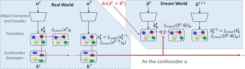
Figure 2: An illustration of the proposed Causal World Models.

Our starting point is learning a set of object-oriented state abstractions and models the transition using graph neural networks, which facilitates capturing the structural property of the physical system and tackles the credit-assignment problem faced by most conventional generative WMs. To further improve the discrepancy between state abstractions, the training of CWM is carried out with an energy-based hinge loss (LeCun et al., 2006), which scores positive against negative experiences in the form of transition dynamics and propose to learn the transition dynamics in the latent space directly. Lastly, we introduce our confounder estimator using a set of recurrent neural networks.

Object Extractor and Encoder

To avoid the credit-assignment problem introduced by generative-based world models, which optimize a prediction or reconstruction objective in pixel space and thereby could ignore visually small but informative features for predicting the future (such as, for instance, a bullet in an Atari game (Łukasz Kaiser et al., 2020)), CWM learns a set of abstract state values ${\mathbf{s}}^{t}\in\mathcal{S}\equiv\mathbb{R}^{D}$ for each object in ${\bm{o}}^{t}\in\mathcal{O}$. Formally, we have an encoder $f_{\text{enc}}:\mathcal{O}\rightarrow K\times\mathcal{S}$ which maps observation to $K$ abstract state representations. The choice of $K$ is a hyperparameter and we conduct ablation study on its influence in Appendix D. A simple implementation of $f_{\text{enc}}$ consists of two modules: 1) a CNN taking ${\bm{o}}^{t}$ as input with $K$ feature maps in its last layer corresponding to $K$ object slots, respectively; and 2) an MLP taking each feature map as input and producing the corresponding abstract state representation ${\bm{s}}^{t}_{k}$ with $k\in\{1,2,\dots,K\}$. Note that choosing other advanced unsupervised object representation learning methods for $f_{\text{enc}}$ is a straightforward extension. For example, an alternative choice could be the Transporter (Kulkarni et al., 2019), which is used for learning concise geometric object representations in terms of image-space coordinates in a fully unsupervised manner.

Transition Estimator

We formulate the transition model of CWM as $f_{\text{trans}}:K\times\mathcal{S}\rightarrow K\times\mathcal{S}$ operating on abstract state representations ${\bm{s}}^{t}$. In this paper, we implement $f_{\text{trans}}$ as a graph neural network (Battaglia et al., 2018; Kipf & Welling, 2017; Li et al., 2016; Scarselli et al., 2009), which allows us to model pairwise interactions between object states while being invariant to the order in which objects are represented. The transition model $f_{\text{trans}}$ takes as input the tuple of abstract object representations ${\bm{s}}^{t}=({\bm{s}}^{t}_{1},\dots,{\bm{s}}^{t}_{K})$ and predicts updates $\Delta{\bm{s}}^{t}=(\Delta{\bm{s}}^{t}_{1},\dots,\Delta{\bm{s}}^{t}_{K})$. which are used to obtain the next abstract state representations via a combination function $f_{\text{comb}}(\cdot,\cdot)$. In this work we simply choose $f_{\text{comb}}$ as an addition function, i.e., $f_{\text{comb}}\left({\bm{s}}^{t},f_{\text{trans}}({\bm{s}}^{t})\right)={\bm{s}}^{t}+\Delta{\bm{s}}^{t}$. Alternatively, one could model the combination using other graph embedding methods (Nickel et al., 2011; Trouillon et al., 2016). The graph neural network consists of node update functions $f_{\text{trans-node}}$ and edge update functions $f_{\text{trans-edge}}$ with shared parameters across all nodes and edges. These functions are implemented as MLPs and we choose the message passing updates as $\Delta{\bm{s}}^{t}_{j}=f_{\text{trans-node}}([{\bm{s}}^{t}_{j},\textstyle\sum_{i\neq j}{\bm{e}}_{i,j}^{t}])$, where ${\bm{e}}_{i,j}^{t}=f_{\text{trans-edge}}([{\bm{s}}^{t}_{i},{\bm{s}}^{t}_{j}])$ is an intermediate representation of the interaction between nodes $i$ and $j$. We denote the output of the transition model for the $k$-th object as $\Delta{\bm{s}}^{t}_{k}=f_{\text{trans}}({\bm{s}}^{t})_{k}$ in the following.

Training Objective

To further improve the discrepancy between state abstractions, the training of CWM is carried out with an energy-based hinge loss (LeCun et al., 2006), which scores positive and negative samples in a different direction and has been widely used in the field of graph representation learning (Bordes et al., 2013; Grover & Leskovec, 2016; Perozzi et al., 2014; Schlichtkrull et al., 2018; Velickovic et al., 2018). We define the energy of two consecutive state variables and the energy of the negative sample as

$$\begin{split}\mathcal{H}&=\frac{1}{K}\sum\nolimits_{k=1}^{K}d(f_{\text{comb}}\left({\bm{s}}^{t}_{k},f_{\text{trans}}({\bm{s}}^{t})_{k}\right),{\bm{s}}^{t+1}_{k})\text{ ,}\\ \tilde{\mathcal{H}}&=\frac{1}{K}\sum\nolimits_{k=1}^{K}d(\tilde{{\bm{s}}}^{t}_{k},{\bm{s}}^{t+1}_{k}),\end{split}$$ (2)

where $d(\cdot,\cdot)$ denotes the squared Euclidean distance and $\tilde{{\bm{s}}}^{t}$ denotes a corrupted abstract state encoded by $\tilde{{\bm{s}}}^{t}=f_{\text{enc}}(\tilde{{\bm{o}}}^{t})$ using a random sample $\tilde{{\bm{o}}}_{t}$ from the experience buffer. The objective of CWM then takes the following energy-based hinge loss form as:

$$\mathcal{L}=\mathcal{H}+\max(0,\gamma-\tilde{\mathcal{H}})\,,$$ (3)

where margin $\gamma$ is a hyperparameter. The overall loss is to be understood as an expectation of the above over samples from the experience buffer.

Deconfounding

We develop CWM by learning an estimator $\hat{{\mathbf{u}}}$ to approximate the latent representation of the confounders ${\mathbf{u}}_{k}$ for each object $k$. The estimator $\hat{{\mathbf{u}}}$ is trained end-to-end by optimizing the counterfactual prediction loss through a recurrent neural network, which takes as input the sequence of abstract state variables ${\bm{s}}^{0:{T}}_{k}$. Concretely, we run a dedicated RNN with GRU (Cho et al., 2014) $f_{\phi}$ for each object trajectory ${\bm{s}}^{0:{T}}_{k}$ and keep the last hidden state $h^{T}_{k}=f_{\phi}({\bm{s}}^{0:{T}}_{k})$ as the estimate of the latent representation of the confounders, i.e., $\hat{{\mathbf{u}}}_{k}\triangleq h^{T}_{k}$. We follow the convention of sharing the parameters of $f_{\phi}$ over $K$ objects (Baradel et al., 2020), which makes the model invariant to the number of objects. The confounders estimation is then fed into the dream world model by concatinating (shown as [:] in Figure 2) with ${\bm{s}}^{t}$ before the transition estimator to predict the alternative futures after do-intervention.

3.5 Doubly Robust Learning from Historical Observations

In real-world scenarios, models trying to approximate the counterfactual distribution will be biased because of the inadequate counterfactual records. For example, in the physical dynamics scenario with continuous intervention space, historical trajectories satisfy a certain but unknown distribution which corresponds to the historical sampling policy. It cannot be discretely considered like propensity scores in traditional IPS function (Swaminathan & Joachims, 2015a), since it may involve an unavoidable variance. To minimize counterfactual risk when training CWMs, we choose the propensity score as the historical sampling policy of selected intervention $p(\mathbf{s^{0}})$ represented by a density function. Inspired by the doubly robust (DR) estimator, our estimator is set as below.

Definition 2.

Let $p({\bm{s}}^{0})$ denotes the history observation distribution (propensity score) on $t_{0}$, and $O(\mathbf{s}|t)=\delta(\mathbf{s}=\mathbf{s^{t}})$ denotes the observation indicator function (i.e. when $\mathbf{s}=\mathbf{s^{t}}$, the $O(\mathbf{s^{t}}|t)=1$), the Doubly Robust prediction of ${\bm{s}}^{t+1}$ is

$$\begin{split}\hat{{\bm{s}}}_{DR}^{t+1}({\bm{s}}^{t})&=\frac{O(s={\bm{s}}^{0}|t_{0})}{p({\bm{s}}^{0})}({\bm{s}}^{t+1}-{\bm{s}}^{t}-\hat{f}_{\text{trans}}({\bm{s}}^{t}))\\ &\quad\quad+({\bm{s}}^{t}+\hat{f}_{\text{trans}}({\bm{s}}^{t}))\end{split}$$ (4)

Proposition 1.

Given the propensity score $p(\mathbf{s^{0}})$, the doubly robust oracle is unbiased against the true trajectory observation, i.e., $\mathbb{E}[\hat{\mathbf{s}}_{DR}^{t+1}]=\mathbf{s^{t+1}}$.

See Appendix B for the proof. We arrive at the doubly robust objective function for CWMs as:

$$\mathcal{L}_{DR}=\frac{1}{K}\sum\nolimits_{k=1}^{K}d(\hat{{\bm{s}}}_{DR,k}^{t+1},{\bm{s}}^{t+1}_{k})+max(0,\gamma-\tilde{\mathcal{H}}),$$ (5)

where $\gamma$ is a free parameter and $\tilde{\mathcal{H}}$ is the energy of negative samples as described in Equation 3.

4 Experiment

We compare our Causal World Models (CWMs) against the state-of-the-art conventional world models (WMs) (Kipf et al., 2020) in two benchmarks, CoPhy (Baradel et al., 2020) and PHYRE (Bakhtin et al., 2019), to evaluate the quality and the usability of the created dream environment, respectively. We empirically evaluate our method and show reductions in sample complexities for reinforcement learning tasks and improvements in counterfactual physical reasoning predictions.

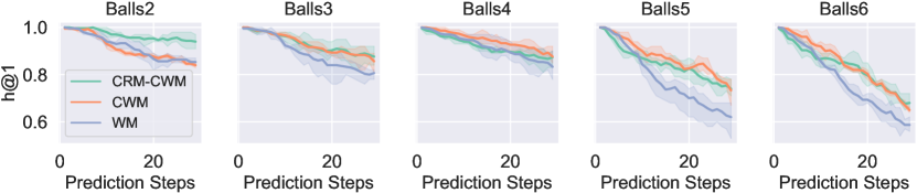
Figure 3: (H@1) Ranking results for multi-step prediction in latent space in different environments. Our models (CWM and CRM-CWM) consistently achieve the best result.

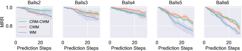
Figure 4: (MRR) Ranking results for multi-step prediction in latent space in different environments. Our models (CWM and CRM-CWM) consistently achieve the best result.

4.1 Dream Quality

Environment Settings

We conduct our experiments on CoPhy (Baradel et al., 2020), a recently proposed benchmark suite for counterfactual reasoning of physical dynamics from raw visual input, which contains $K$ balls $(K=2,3,4,5,6)$ initialized with a random position and velocity. The world is parameterized by a set of visually unobservable quantities, or confounders, consisting of ball masses and the friction coefficients. As described in Section 3.2, the training data of CoPhy is a tuple of two trajectories: the real-world trajectory ${\bm{o}}^{0:{T}}$ and the counterfactual trajectory $\bar{{\bm{o}}}^{0:{T}^{\prime}}$ after one of the two do-operators: ball displacement or removal. The model is evaluated by its dream creation quality, i.e., the prediction of the counterfactual outcome $\bar{{\bm{o}}}^{1:{T}^{\prime}}$ given real-world trajectory ${\bm{o}}^{0:{T}}$ and the intervened initial observation $\bar{{\bm{o}}}^{0}$. In our experiments, we sampled $700$ tuples of data from the CoPhy benchmark as the training set and $300$ tuples of data as the test set. All trajectories contains observations for $29$ time steps. We follow the convention of using two ranking metrics: (1) Hits @ Rank 1 (H@1) and (2) Mean Reciprocal Rank (MRR) to evaluate model performance directly in the latent space (Bordes et al., 2013; Kipf et al., 2020). The predicted abstract state representation is compared to the encoded ground truth observation and a set of reference states, which are encoded from random observations sampled from the experience buffer. We report the average scores over the test set for different prediction steps $T^{\prime}$. Details on evaluation metrics can be found in Appendix C.

Model Settings

We compare with the state-of-the-art world model (WMs) variations for representation learning in environments with compositional structure (Kipf et al., 2020). The counterfactual prediction (dream creation) of WMs is implemented by simply concatenating ${\bm{o}}^{t}$ with $\bar{{\bm{o}}}^{t}$ following the causal graph in Figure 1(a). We propose two variations of Causal World Models (CWMs): the original CWMs described in Section 3.4 and the unbiased-augmented CRM-CWMs using counterfactual risk minimization as described in Section 3.5. CRM-CWMs work by estimating a Gaussian probability density function of historical samples on the training set. This density function is then used as the propensity score for Equation 5. All models share the same setting for the object extractor, encoder, and the transition estimator. Details on architecture and hyperparameters setting can be found in Appendix D.1. We choose over different number of slots $\{2,3,4,5,6\}$ (the hyperparameter $K$ as described in Section 3.4) and present the result with the best configuration for each model respectively. Ablation study on the number of slots can be found in Appendix E.

Result Analysis

We firstly show the qualitative example of predicted dream trajectories of WMs and CWMs in the latent space of the 6-ball CoPhy environment in  Figure LABEL:subfig:traj_wm and Figure LABEL:subfig:traj_cwm, respectively. Trajectories are projected to two dimensions via PCA and presented with the same scale. The mean squared errors between the predicted state values and ground truth are presented for each episode. We can observe that CWMs reliably predict the trajectories in the dream world without direct supervision, while WMs suffer from a poor counterfactual prediction ability. Further qualitative results can be found in Appendix E. Figure 3 and Figure 4 show the ranking results of predicting unseen future in the dream world in terms of H@1 and MRR metrics respectively. Our proposed CWMs and CRM-CWMs consistently give the best result across all training environments, demonstrating that the estimation of confounders helps counterfactual prediction by modeling the intrinsic environment property. Also, we discover that the conventional WMs are sensitive to the difficulty of environments: the hidden confounders of the environment results in higher variance on such methods learning directly from observational data. On the other hand, our proposed CRM-CSMs consider the historical sample policy and use counterfactual learning to reduce the sampling bias during the learning process, thus achieving the best result among the comparison group.

4.2 Dream Usability

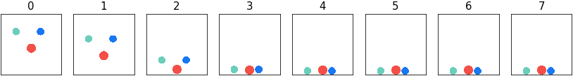
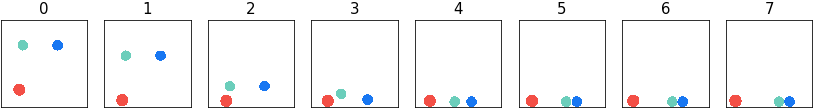
(a) A failed trial: placing the red cannot make the green touch the blue.

(b) A successful trial where the green and blue ball touch each other.

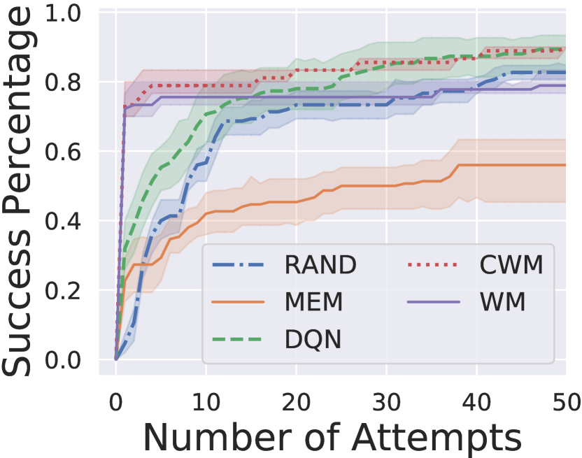
(c)

Figure 5: Example of the PHYRE environment with (a) a failed trial and (b) a successful trial. (c) Percentage of solved tasks with respect to the number of attempts per task on PHYRE environment.

Environment Settings

We evaluate the usability of the created dream world by measuring the number of interactions with the environment needed to achieve the goal in PHYRE (Bakhtin et al., 2019) environment. The task is formulated as a physics puzzle in a simulated 2D world containing multiple objects as shown in Figure 5(b). Each task has a goal state defined as a (subject, relation, object) triplet identifying a relationship between two objects that the agent needs to achieve before it reaches the horizon $T$, e.g., make the green ball touch the blue ball as shown in Figure 5(b). The agent’s action, as well as the intervention, is defined as placing an object into the world before the environment rollout, i.e., $\mathcal{A}=(a_{x},a_{y},a_{r})\equiv\mathbb{R}^{D}\times\mathbb{R}^{D}\times\mathbb{R}^{1}$, where $(a_{x},a_{y})$ and $a_{r}$ represents the object’s location and size respectively. The agent takes no actions during the environment rollout and receives a binary reward indicating whether the goal is satisfied after the simulation. All agents are trained to predict whether a specific action (from the default $100k$ action candidates) can solve a specific task and evaluated by the number of attempts used to solve previously unseen tasks with a given set of action candidates.

Model Settings

We compare with three baseline agents: (1) random agent (RAND), which samples actions uniformly at random from action space at test time; (2) non-parametric “memorized” agent (MEM), which computes the fraction of training tasks that a set of actions can solve, sorts the action set according to the successful rate, and tries each action in this order at test time; (3) the Deep Q-network (DQN) agent, which trains a deep network on the offline collected data to predict the reward for an observation-action pair. We use the same setting as described in Section 4.1 for WMs and CWMs and train a separate classifier to predict whether the task is solved given an abstract state value. At test time, WMs and CWMs produce a score through the classifier based on the predicted counterfactual state value for all valid action candidates of each task, and attempt to solve the task in the score order. Details on architecture and hyperparameters setting can be found in Appendix D.2.

Result Analysis

Figure 5(c) presents success-percentage curves on the PHYRE environment averaged over all test tasks and 3 random seeds. It is clear that CWMs agents perform better than WMs in terms of both the sample complexity and the final average success percentage within the trial budget (50 attempts), which demonstrate the importance of deconfounding in physical simulation. Meanwhile, model-based agents (CWMs and WMs) can significantly reduce the sample complexity when compared to model-free counterparts, owing to the fact that learning a model of the world can help to reason about what would happen upon a particular change to a previous attempt. These, in turn, demonstrate the advantage of our model-based approach towards physical reasoning.

5 Conclusion

In this paper, we propose Causal World Models (CWMs) to create a dream world able to predict the alternative future not encountered in the real world in a fully unsupervised manner. By learning an estimator of the latent confounders and optimizing directly within the abstract state space, CWMs outperform state-of-the-art world models in both the reinforcement learning tasks and physical simulation environments. To further reduce the inevitable bias of counterfactual dataset, we also propose a counterfactual risk minimization method for CWMs and demonstrate its effectiveness in learning counterfactual physical dynamics. In the future, we would like to explore CWMs’ ability in a broader range of applications and more complex environments.

Appendix A Simpson’s Paradox in the Medical Treatment Scenario

We include the classical example of Simpson’s Paradox in the medical treatment scenario from Pearl (2009) to demonstrate the wide existence of confounding.

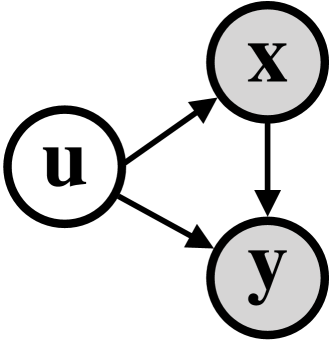
(a)

(b)

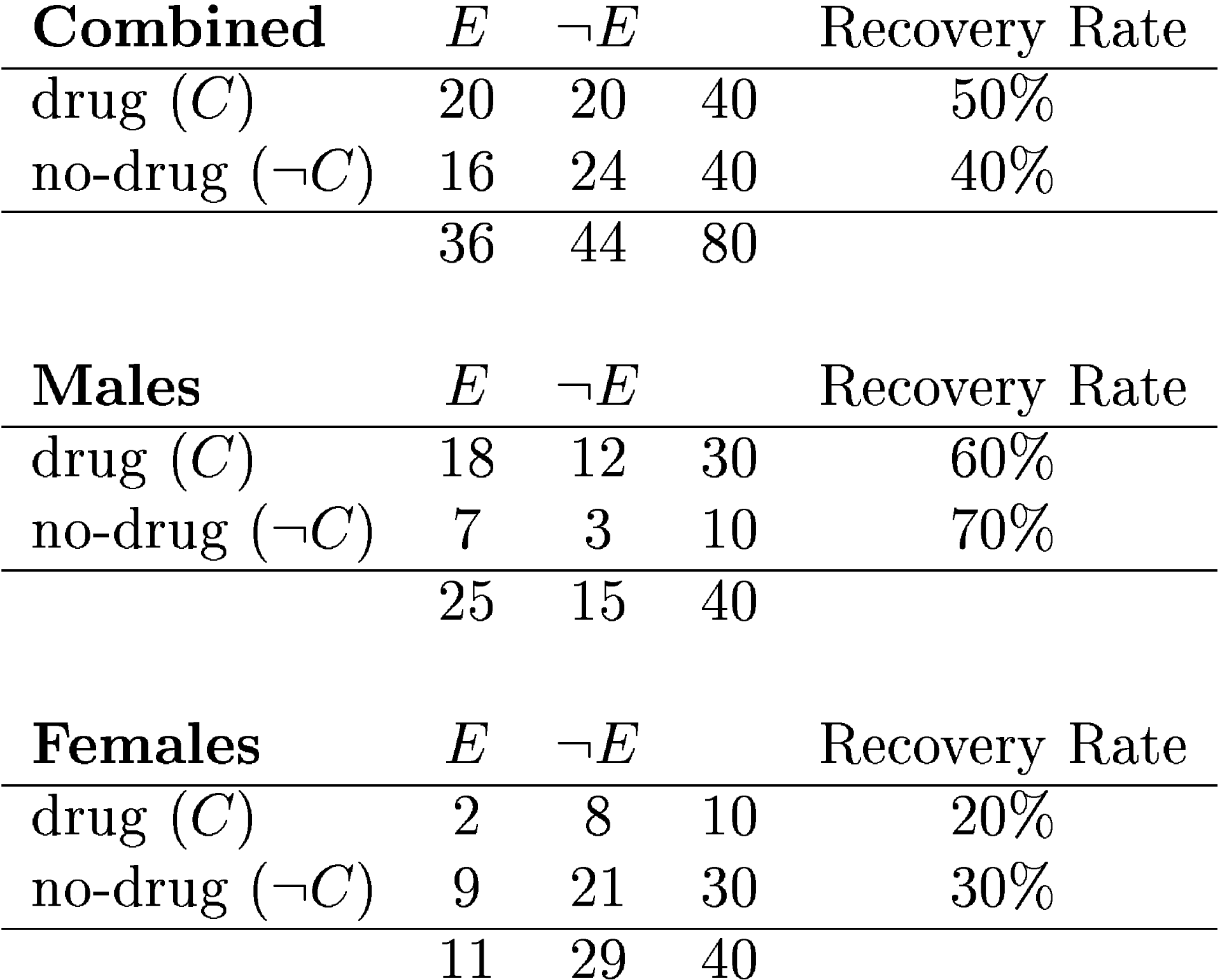
(c) Example from Pearl (2009).

Figure 1: Confounding in medical scenarios. We present the simplified causal graph of the transition model used by (a) conventional World Models (WMs); (b) Causal World Models (CWMs), with the consideration of confounding. ${\mathbf{x}}$ represents the treatment (taking drug or not), ${\mathbf{y}}$ represents the recovery, and ${\mathbf{u}}$ represents the gender (male or female).

Consider the example where ${\mathbf{y}}$ is the observational recovery rate and ${\mathbf{x}}$ is taking a drug as the treatment. As illustrated in Figure 1(c), Pearl (2009) shows that the overall recovery rate of all patients increased from $40\%$ to $50\%$ after the treatment, while the drug appeared to be harmful to both male (recovery rate dropped from $70\%$ to $60\%$) and female patients (recovery rate dropped from $30\%$ to $20\%$) respectively. Simply using the causal chain of conventional world models (WMs) (shown as in Figure 1(b)) will lead to the above Simpson’s paradox (Simpson, 1951), which refers to the phenomenon that a trend appears in several different groups of data but disappears or reverses when these groups are combined. An intuitive explanation for this phenomenon is that females are more vulnerable to the disease and are much more likely to die without the treatment, resulting in that no treatment looks worse than taking the drug overall. This intuition leads us to the assumption of the true underlying causal graph of the example shown in Figure 1(b), which takes confounding ${\mathbf{u}}$ into account as the gender affects both the treatment and recovery.

Appendix B Proof of Proposition 1

Proof: Let ${\bm{s}}^{t}$ be the $t$-th latent state of trajectory $k$.

$$\mathbb{E}(\hat{{\bm{s}}}_{DR}^{t+1}({\bm{s}}^{t})|{\bm{s}}^{0}) =\mathbb{E}(\frac{O({\bm{s}}^{0}|t=0)}{p({\bm{s}}^{0})}({\bm{s}}^{t+1}-{\bm{s}}^{t}-\hat{f}_{\text{trans}}({\bm{s}}^{t}))+({\bm{s}}^{t}+\hat{f}_{\text{trans}}({\bm{s}}^{t}))|{\bm{s}}^{0})$$

$$=\mathbb{E}(\frac{O({\bm{s}}^{0}|t=0)}{p({\bm{s}}^{0})})\mathbb{E}({\bm{s}}^{t+1}-{\bm{s}}^{t}-\hat{f}_{\text{trans}}({\bm{s}}^{t})|{\bm{s}}^{0})+\mathbb{E}({\bm{s}}^{t}+\hat{f}_{\text{trans}}({\bm{s}}^{t})|{\bm{s}}^{0})$$

$$={\bm{s}}^{t+1}$$

Appendix C Evaluation Metrics for the Dream Quality Experiment

We follow the convention of using ranking metrics to evaluate model performance directly in latent space (Bordes et al., 2013; Kipf et al., 2020). The predicted abstract state representation is compared to the encoded ground truth observation and a set of reference states, which are encoded from random observations sampled from the experience buffer. We measure and report the following two metrics:

Hits @ Rank 1 (H@1)

H@1 is a binary score measuring whether the rank of predicted abstract state representation equals to 1 after ranking all the reference state representations by distance to the ground truth.

Mean Reciprocal Rank (MRR)

MRR measures the inverse average rank of all the by $MRR=\frac{1}{N}\sum_{n}\frac{1}{\text{rank}_{n}}$, where $\text{rank}_{n}$ is the rank of $n$-th sample.

We report the average of these scores over the test set for different prediction steps $T^{\prime}$.

Appendix D Architecture and Hyperparameter Settings

D.1 Dream Quality Experiments

We train all models on an experience buffer obtained by running a random policy on the respective environment. We choose $700$ episodes with $29$ environment steps each for the training set and $300$ episodes with $29$ steps each for the test set. All observations for this benchmark have been rendered into the visual space (RGB) at a resolution of $448\times 448$ pixels with PyBullet (Coumans & Bai, 2016–2019) and we resize the observation to $50\times 50$ pixels each.

All models are trained for $200$ epochs using the Adam (Kingma & Ba, 2014) optimizer with a learning rate of $5e-4$ and a batch size of $25$ (due to the relatively large size of each training tuple). All experiments were completed on a single NVIDIA GeForce GTX 1080 Ti GPU in under 2 hours.

D.1.1 WMs

Object Extractor

We choose the object extractor as the following.

1. $9\times 9$ conv. 32 LeakyReLU (Xu et al., 2015). padding 4. stride 1. BatchNorm (Ioffe & Szegedy, 2015)

2. $5\times 5$ conv. $K$ Sigmoid. padding 0. stride 5. BatchNorm

Object Encoder

After reshaping/flattening the output of the object extractor, we obtain a $100$-dim vector representation per object. The object encoder is an MLP using the following architecture.

1. fully connected. 512 ReLU.

2. fully connected. 512 ReLU. LayerNorm (Ba et al., 2016)

3. fully connected. 4.

Transition Estimator

Both the node and the edge model in the GNN-based transition model are MLPs with the same architecture as the above object encoder module.

Loss Function

We choose the margin in the hinge loss as $\gamma=1$. We further multiply the squared Euclidean distance $d(x,y)$ in the loss function with a factor of $0.5/\sigma^{2}$ with $\sigma=0.5$ to control the spread of the embeddings.

D.1.2 CWMs

Confounder Estimator

We choose the confounder estimator $f_{\phi}$ as a GRU (Cho et al., 2014) with 2 layers and a hidden state of dimension 32.

All other settings are the same as the conventional world models in Appendix D.1.1 and we concatenate the abstract state with the estimated confounder to feed into the transition model.

D.1.3 CRM-CWMs

Propensity Score Estimation We estimate the propensity score as a Gaussian Distribution density function, i.e., $f(x)=\frac{1}{\sigma\sqrt{2\pi}}e^{-\frac{(x-\mu)^{2}}{2\sigma^{2}}},$ where $x$ are all the observations from the training set. We use Equation 5 as our training objective. All other settings are the same as the CWMs in Appendix D.1.2.

D.2 Dream Usability Experiments

We train all models on an experience buffer obtained by running a random policy on the respective environment. We choose $70$ tasks as the training set and $30$ tasks as the test set. At test time, all agents (except the random agent) rank the same set of $200$ actions on each task and propose the highest-scoring actions for that task as solution attempts. In the PHYRE environment, the observation is a $256\times 256$ image with one of $7$ colors at each pixel, which encodes properties of each body and the goal. We map this observation into a $7$-channel image for input to the CNN; each colored pixel in the image yields a $7$D one-hot vector.

D.2.1 DQN

The DQN agent comprises three parts:

Action Encoder

The action encoder transforms the 3D action $(a_{x},a_{y},a_{r})$ as described in Section 4.2 using the following structure:

1. fully connected. 256 ReLU.

2. fully connected. 128.

Observation Encoder

The observation encoder transforms the observation image into a hidden representation using a CNN with the following structure:

1. $1\times 1$ conv. 3 ReLU. padding 0. stride 1. BatchNorm

2. $7\times 7$ conv. $64$ ReLU. padding 3. stride 4. BatchNorm

3. $5\times 5$ conv. $64$ ReLU. padding 2. stride 2. BatchNorm

4. $5\times 5$ conv. $64$ ReLU. padding 2. stride 2. BatchNorm

5. $5\times 5$ conv. $64$ ReLU. padding 2. stride 2. BatchNorm

6. $5\times 5$ conv. $128$ ReLU. padding 2. stride 2. BatchNorm

7. $5\times 5$ conv. $128$ ReLU. padding 2. stride 2. BatchNorm

8. $5\times 5$ conv. $128$ ReLU. padding 2. stride 2. BatchNorm

Fusion Module

The fusion module combines the action and observation representations and makes a reward prediction.

The DQN agent network is trained end-to-end using Adam optimizer by minimizing the cross-entropy between the soft prediction and the observed reward. The learning rate for DQN is set as $3e-4$.

D.2.2 WMs

Object Extractor

We choose the object extractor as the following:

1. $1\times 1$ conv. 3 ReLU. padding 0. stride 1. BatchNorm

2. $7\times 7$ conv. $64$ ReLU. padding 3. stride 4. BatchNorm

3. $5\times 5$ conv. $64$ ReLU. padding 2. stride 2. BatchNorm

4. $5\times 5$ conv. $64$ ReLU. padding 2. stride 2. BatchNorm

5. $5\times 5$ conv. $64$ ReLU. padding 2. stride 2. BatchNorm

6. $5\times 5$ conv. $K$ ReLU. padding 2. stride 2. BatchNorm

$K$ is a hyperparameter and we typically set it with heuristic as the number of objects in the task, i.e., $K=3$ for the task in Figure 5(b).

Object Encoder, Transition Function, and the Loss Function

All modules are the same as the setting in Appendix D.1.2.

State Status Classifier

We train a separate classifier to predict whether the task is solved given an abstract state value. The classifier is of the following architecture:

1. fully connected. 256 ReLU.

2. fully connected. 128 ReLU.

3. fully connected. 2.

The classifier network is trained by minimizing the cross-entropy between the soft prediction and the label (state solved or not).

All models are trained for $200$ epochs using the Adam optimizer with a learning rate of $5e-4$ and a batch size of $16$ (due to the relatively large size of each training tuple). All experiments were completed on a single NVIDIA GeForce GTX 1080 Ti GPU in under 6 hours.

D.2.3 CWMs

Confounder Estimator

We choose the confounder estimator as the same setting as described in Appendix D.1.2.

All other settings are the same as the conventional world models in Appendix D.2.2 and we concatenate the abstract state with the estimated confounder to feed into the transition model.

Appendix E Additional Experiment Results

E.1 Qualitative Examples of Dream Quality Experiments

We present additional dream (counterfactual prediction) trajectories for different environments in Figure 2 through Figure 6.

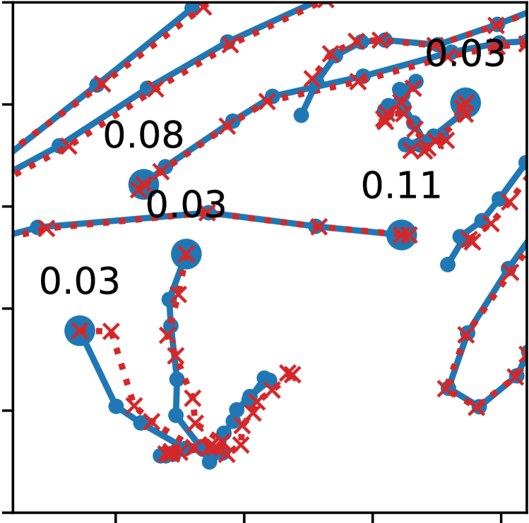
(a) WMs: $0.056$$\pm 0.037$

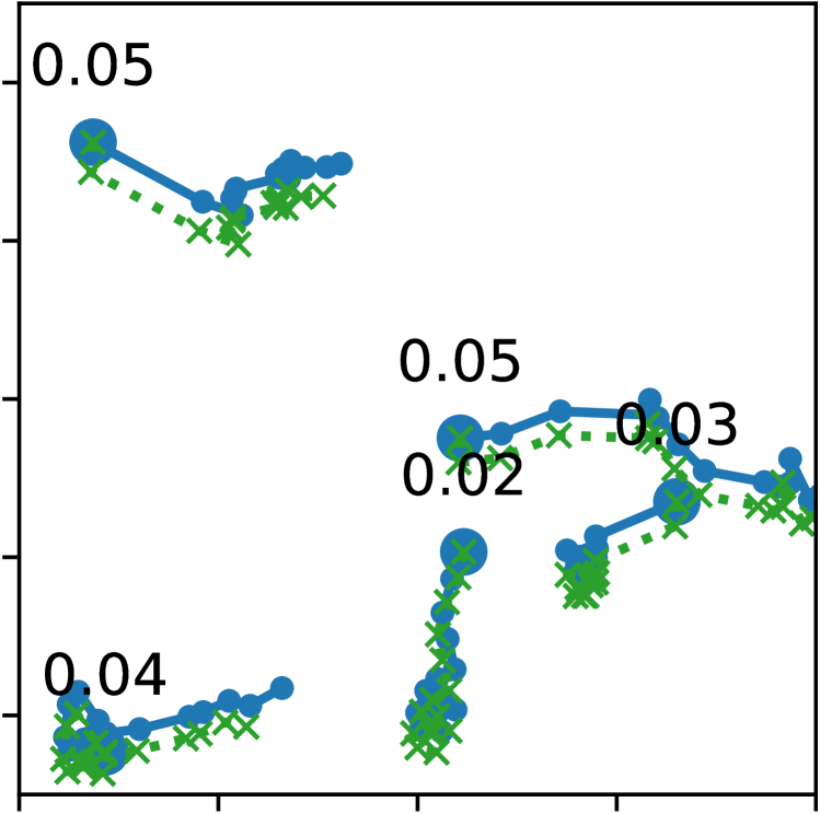
(b) CWMs: $0.038$$\pm 0.013$

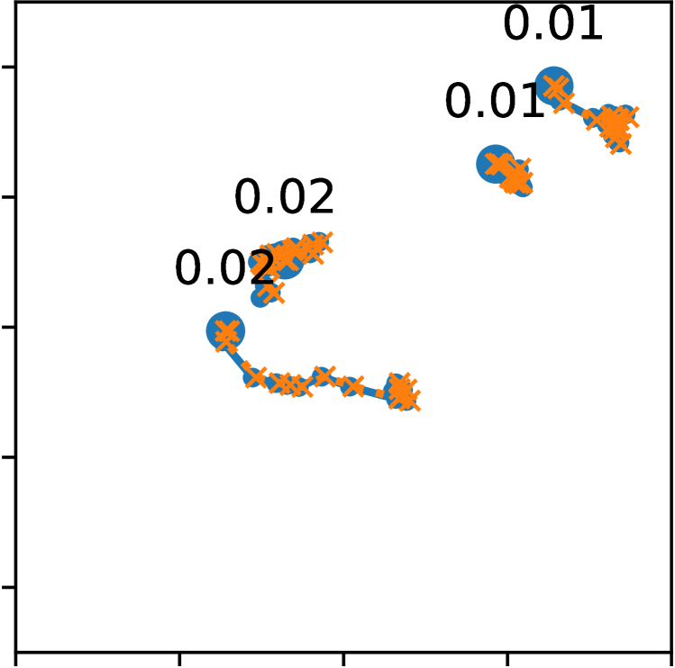
(c) CRM-CWMs: $0.015$$\pm 0.006$

Figure 2: The dream (counterfactual prediction) trajectories on (a) WMs (cross with red dotted lines), (b) CWMs (cross with green dotted lines), and (c) CRM-CWMs (cross with orange dotted lines) along with the ground truth (circle with blue solid lines) in the latent space of the 2-ball CoPhy environment. Trajectories are projected to two dimensions via PCA and presented with the same scale. The MSE between the predicted state values and the ground truth are presented for each episode.

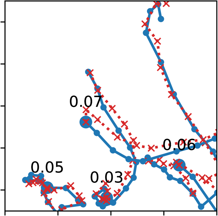
(a) WMs: $0.053$$\pm 0.017$

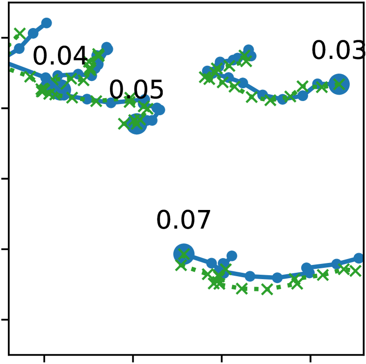
(b) CWMs: $0.048$$\pm 0.017$

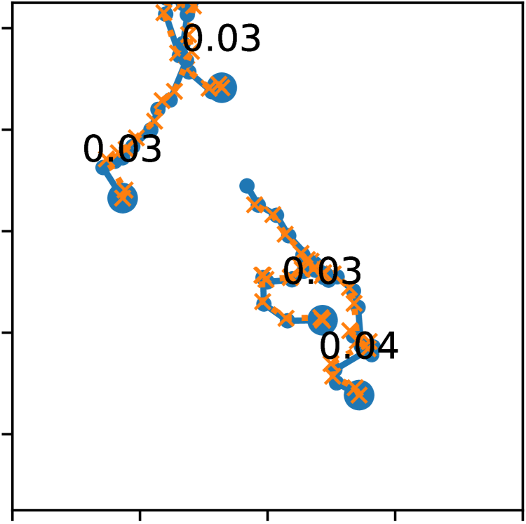
(c) CRM-CWMs: $0.033$$\pm 0.005$

Figure 3: The dream (counterfactual prediction) trajectories on (a) WMs (cross with red dotted lines), (b) CWMs (cross with green dotted lines), and (c) CRM-CWMs (cross with orange dotted lines) along with the ground truth (circle with blue solid lines) in the latent space of the 3-ball CoPhy environment. Trajectories are projected to two dimensions via PCA and presented with the same scale. The MSE between the predicted state values and the ground truth are presented for each episode.

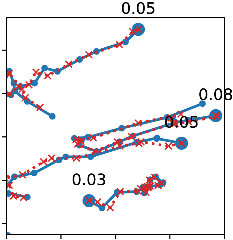
(a) WMs: $0.053$$\pm 0.021$

(b) CWMs: $0.027$$\pm 0.006$

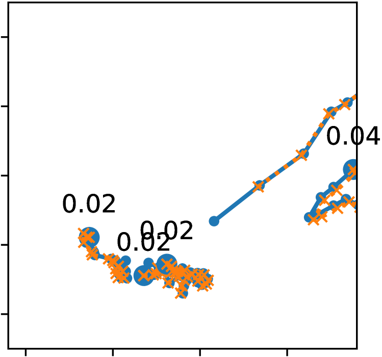
(c) CRM-CWMs: $0.025$$\pm 0.01$

Figure 4: The dream (counterfactual prediction) trajectories on (a) WMs (cross with red dotted lines), (b) CWMs (cross with green dotted lines), and (c) CRM-CWMs (cross with orange dotted lines) along with the ground truth (circle with blue solid lines) in the latent space of the 4-ball CoPhy environment. Trajectories are projected to two dimensions via PCA and presented with the same scale. The MSE between the predicted state values and the ground truth are presented for each episode.

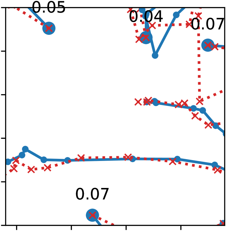
(a) WMs: $0.058$$\pm 0.015$

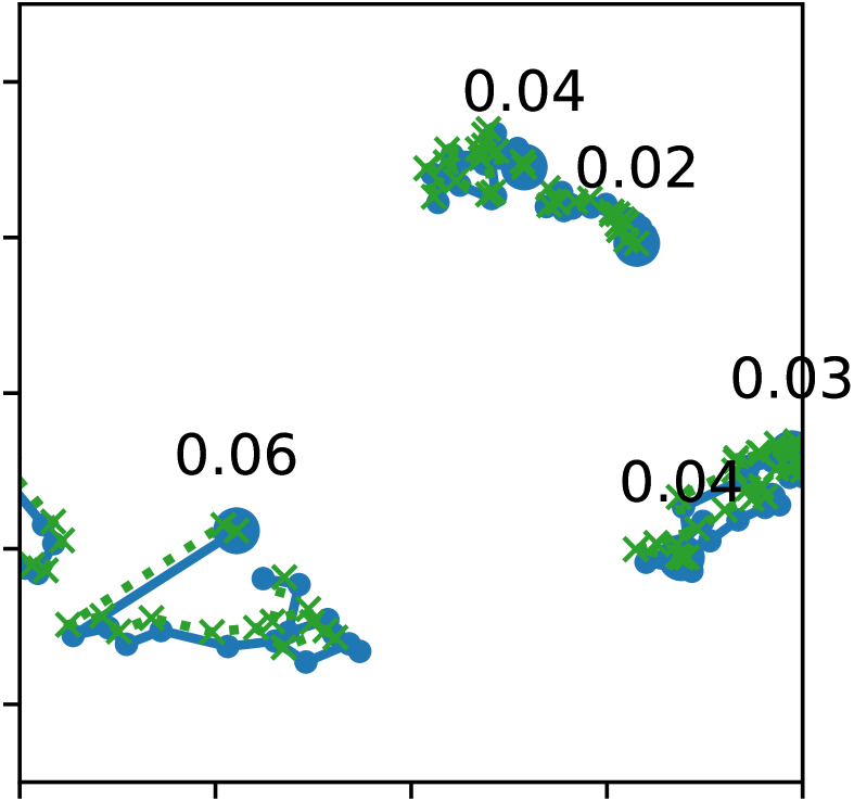
(b) CWMs: $0.038$$\pm 0.015$

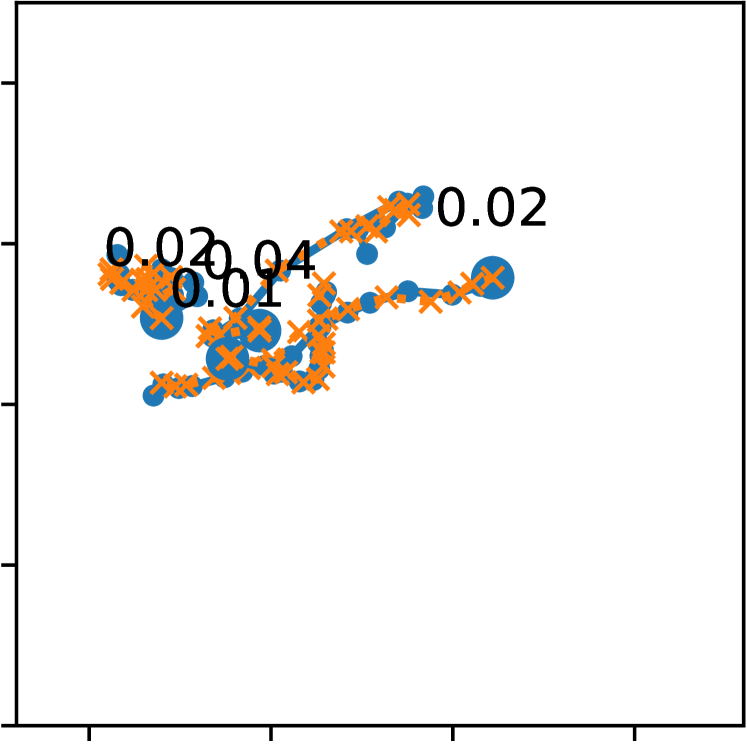
(c) CRM-CWMs: $0.023$$\pm 0.013$

Figure 5: The dream (counterfactual prediction) trajectories on (a) WMs (cross with red dotted lines), (b) CWMs (cross with green dotted lines), and (c) CRM-CWMs (cross with orange dotted lines) along with the ground truth (circle with blue solid lines) in the latent space of the 5-ball CoPhy environment. Trajectories are projected to two dimensions via PCA and presented with the same scale. The MSE between the predicted state values and the ground truth are presented for each episode.

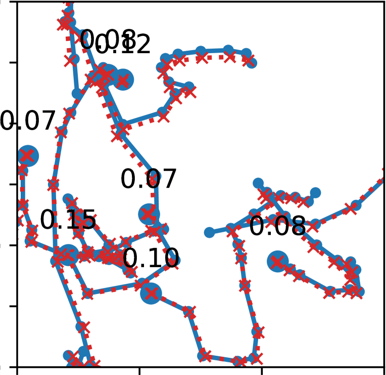
(a) WMs: $0.096$$\pm 0.030$

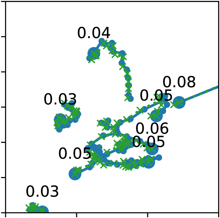
(b) CWMs: $0.049$$\pm 0.016$

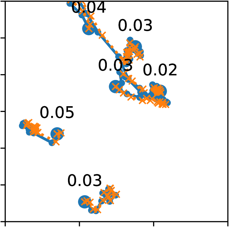
(c) CRM-CWMs: $0.033$$\pm 0.010$

Figure 6: The dream (counterfactual prediction) trajectories on (a) WMs (cross with red dotted lines), (b) CWMs (cross with green dotted lines), and (c) CRM-CWMs (cross with orange dotted lines) along with the ground truth (circle with blue solid lines) in the latent space of the 6-ball CoPhy environment. Trajectories are projected to two dimensions via PCA and presented with the same scale. The MSE between the predicted state values and the ground truth are presented for each episode.

E.2 Ablation Study on the Choice of $K$ in Dream Quality Experiments

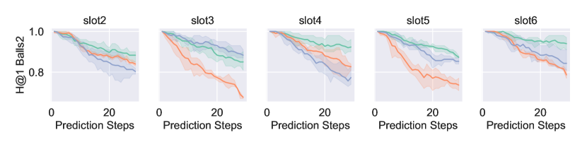
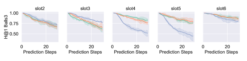
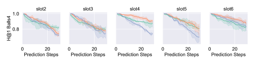
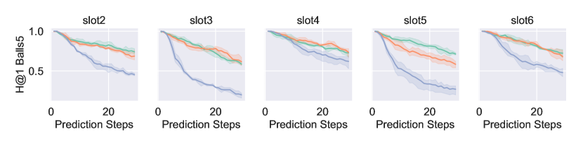
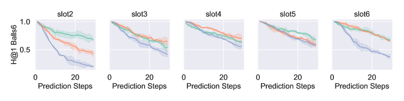
Figure 7: (H@1) Ranking results for multi-step prediction in latent space with different slot (K) variations.

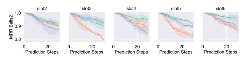
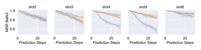
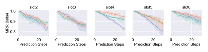
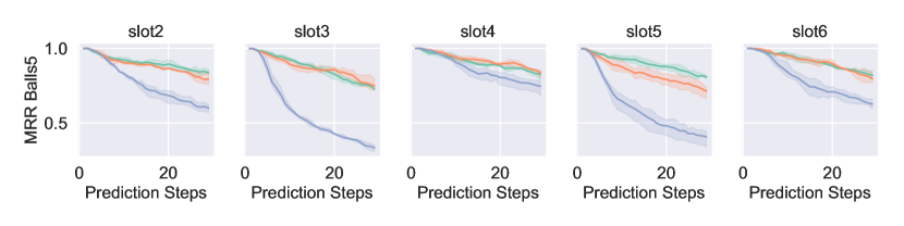
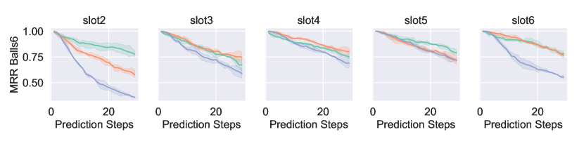
Figure 8: (MRR) Ranking results for multi-step prediction in latent space with different slot (K) variations. Our model (Causal SWM) consistently achieves the best result.

From experimental results, we also discover some insights about parameter tuning. With the increasing number of balls in the environment, all methods have been struggling to make good long term predictions. Although results in Figure 3 and Figure 4 of the main paper are presented using the best configuration of number of object slots $K$ for each model, results in Figure 7 and Figure 8 show that our proposed CWMs and CRM-CWMs benefit from using a larger number of slots in all environments. This finding suggests that using a large number of slots $K$ might be a good choice when dealing with a new environment without any prior information.

References

- Alaa & van der Schaar (2019) Alaa, A. M. and van der Schaar, M. Validating causal inference models via influence functions. In Chaudhuri, K. and Salakhutdinov, R. (eds.), Proceedings of the 36th International Conference on Machine Learning, ICML 2019, 9-15 June 2019, Long Beach, California, USA, volume 97 of Proceedings of Machine Learning Research, pp. 191–201. PMLR, 2019.
- Athey & Wager (2017) Athey, S. and Wager, S. Efficient policy learning. arXiv preprint arXiv:1702.02896, 2017.
- Ba et al. (2016) Ba, J. L., Kiros, J. R., and Hinton, G. E. Layer normalization. arXiv preprint arXiv:1607.06450, 2016.
- Bakhtin et al. (2019) Bakhtin, A., van der Maaten, L., Johnson, J., Gustafson, L., and Girshick, R. Phyre: A new benchmark for physical reasoning. In Advances in Neural Information Processing Systems, pp. 5083–5094, 2019.
- Balke & Pearl (1994) Balke, A. and Pearl, J. Counterfactual probabilities: Computational methods, bounds and applications. In Proceedings of the Tenth International Conference on Uncertainty in Artificial Intelligence, UAI’94, pp. 46–54, San Francisco, CA, USA, 1994. Morgan Kaufmann Publishers Inc. ISBN 1558603328.
- Balke & Pearl (1995) Balke, A. and Pearl, J. Counterfactuals and policy analysis in structural models. In Besnard, P. and Hanks, S. (eds.), UAI ’95: Proceedings of the Eleventh Annual Conference on Uncertainty in Artificial Intelligence, Montreal, Quebec, Canada, August 18-20, 1995, pp. 11–18. Morgan Kaufmann, 1995.
- Baradel et al. (2020) Baradel, F., Neverova, N., Mille, J., Mori, G., and Wolf, C. Cophy: Counterfactual learning of physical dynamics. In International Conference on Learning Representations, 2020. URL https://openreview.net/forum?id=SkeyppEFvS.
- Battaglia et al. (2016) Battaglia, P., Pascanu, R., Lai, M., Jimenez Rezende, D., and kavukcuoglu, k. Interaction networks for learning about objects, relations and physics. In Lee, D. D., Sugiyama, M., Luxburg, U. V., Guyon, I., and Garnett, R. (eds.), Advances in Neural Information Processing Systems 29, pp. 4502–4510. Curran Associates, Inc., 2016.
- Battaglia et al. (2018) Battaglia, P. W., Hamrick, J. B., Bapst, V., Sanchez-Gonzalez, A., Zambaldi, V. F., Malinowski, M., Tacchetti, A., Raposo, D., Santoro, A., Faulkner, R., Gülçehre, Ç., Song, H. F., Ballard, A. J., Gilmer, J., Dahl, G. E., Vaswani, A., Allen, K. R., Nash, C., Langston, V., Dyer, C., Heess, N., Wierstra, D., Kohli, P., Botvinick, M., Vinyals, O., Li, Y., and Pascanu, R. Relational inductive biases, deep learning, and graph networks. CoRR, abs/1806.01261, 2018.
- Bordes et al. (2013) Bordes, A., Usunier, N., Garcia-Duran, A., Weston, J., and Yakhnenko, O. Translating embeddings for modeling multi-relational data. In Advances in neural information processing systems, pp. 2787–2795, 2013.
- Burgess et al. (2019) Burgess, C. P., Matthey, L., Watters, N., Kabra, R., Higgins, I., Botvinick, M. M., and Lerchner, A. Monet: Unsupervised scene decomposition and representation. ArXiv, abs/1901.11390, 2019.
- Cassel et al. (1976) Cassel, C. M., Särndal, C. E., and Wretman, J. H. Some results on generalized difference estimation and generalized regression estimation for finite populations. Biometrika, 63(3):615–620, 1976.
- Chalupka et al. (2015) Chalupka, K., Perona, P., and Eberhardt, F. Visual causal feature learning. In Proceedings of the Thirty-First Conference on Uncertainty in Artificial Intelligence, UAI’15, pp. 181–190, Arlington, Virginia, USA, 2015. AUAI Press. ISBN 9780996643108.
- Chang et al. (2017) Chang, M., Ullman, T., Torralba, A., and Tenenbaum, J. B. A compositional object-based approach to learning physical dynamics. In 5th International Conference on Learning Representations, ICLR 2017, Toulon, France, April 24-26, 2017, Conference Track Proceedings. OpenReview.net, 2017.
- Cho et al. (2014) Cho, K., van Merrienboer, B., Gülçehre, Ç., Bahdanau, D., Bougares, F., Schwenk, H., and Bengio, Y. Learning phrase representations using RNN encoder-decoder for statistical machine translation. In Moschitti, A., Pang, B., and Daelemans, W. (eds.), Proceedings of the 2014 Conference on Empirical Methods in Natural Language Processing, EMNLP 2014, October 25-29, 2014, Doha, Qatar, A meeting of SIGDAT, a Special Interest Group of the ACL, pp. 1724–1734. ACL, 2014. doi: 10.3115/v1/d14-1179. URL https://doi.org/10.3115/v1/d14-1179.
- Coumans & Bai (2016–2019) Coumans, E. and Bai, Y. Pybullet, a python module for physics simulation for games, robotics and machine learning. http://pybullet.org, 2016–2019.
- Dudík et al. (2011) Dudík, M., Langford, J., and Li, L. Doubly robust policy evaluation and learning. arXiv preprint arXiv:1103.4601, 2011.
- Engelcke et al. (2020) Engelcke, M., Kosiorek, A. R., Jones, O. P., and Posner, I. Genesis: Generative scene inference and sampling with object-centric latent representations. In International Conference on Learning Representations, 2020. URL https://openreview.net/forum?id=BkxfaTVFwH.
- Eslami et al. (2016) Eslami, S. M. A., Heess, N., Weber, T., Tassa, Y., Szepesvari, D., Kavukcuoglu, K., and Hinton, G. E. Attend, infer, repeat: Fast scene understanding with generative models. In Proceedings of the 30th International Conference on Neural Information Processing Systems, NIPS’16, pp. 3233–3241, Red Hook, NY, USA, 2016. Curran Associates Inc. ISBN 9781510838819.
- Garnelo et al. (2016) Garnelo, M., Arulkumaran, K., and Shanahan, M. Towards deep symbolic reinforcement learning. arXiv preprint arXiv:1609.05518, 2016.
- Greff et al. (2017) Greff, K., van Steenkiste, S., and Schmidhuber, J. Neural expectation maximization. In Advances in Neural Information Processing Systems, pp. 6691–6701, 2017.
- Greff et al. (2019) Greff, K., Kaufmann, R. L., Kabra, R., Watters, N., Burgess, C., Zoran, D., Matthey, L., Botvinick, M., and Lerchner, A. Multi-object representation learning with iterative variational inference. In ICML, pp. 2424–2433, 2019. URL http://proceedings.mlr.press/v97/greff19a.html.
- Grover & Leskovec (2016) Grover, A. and Leskovec, J. node2vec: Scalable feature learning for networks. In Proceedings of the 22nd ACM SIGKDD international conference on Knowledge discovery and data mining, pp. 855–864, 2016.
- Gu et al. (2016) Gu, S., Lillicrap, T., Sutskever, I., and Levine, S. Continuous deep q-learning with model-based acceleration. In ICML, pp. 2829–2838, 2016. URL http://dl.acm.org/citation.cfm?id=3045390.3045688.
- Ha & Schmidhuber (2018) Ha, D. and Schmidhuber, J. Recurrent world models facilitate policy evolution. In Advances in Neural Information Processing Systems 31, pp. 2451–2463. Curran Associates, Inc., 2018. URL https://papers.nips.cc/paper/7512-recurrent-world-models-facilitate-policy-evolution. https://worldmodels.github.io.
- He et al. (2016) He, H., Boyd-Graber, J., Kwok, K., and III, H. D. Opponent modeling in deep reinforcement learning. In Balcan, M. F. and Weinberger, K. Q. (eds.), Proceedings of The 33rd International Conference on Machine Learning, volume 48 of Proceedings of Machine Learning Research, pp. 1804–1813, New York, New York, USA, 20–22 Jun 2016. PMLR.
- Hudson & Manning (2018) Hudson, D. A. and Manning, C. D. Compositional attention networks for machine reasoning. In International Conference on Learning Representations, 2018. URL https://openreview.net/forum?id=S1Euwz-Rb.
- Igl et al. (2018) Igl, M., Zintgraf, L., Le, T. A., Wood, F., and Whiteson, S. Deep variational reinforcement learning for POMDPs. In ICML, pp. 2117–2126, 10–15 Jul 2018. URL http://proceedings.mlr.press/v80/igl18a.html.
- Ioffe & Szegedy (2015) Ioffe, S. and Szegedy, C. Batch normalization: Accelerating deep network training by reducing internal covariate shift. arXiv preprint arXiv:1502.03167, 2015.
- Janner et al. (2019) Janner, M., Levine, S., Freeman, W. T., Tenenbaum, J. B., Finn, C., and Wu, J. Reasoning about physical interactions with object-centric models. In International Conference on Learning Representations, 2019.
- Johnson et al. (2017) Johnson, J., Hariharan, B., Van Der Maaten, L., Hoffman, J., Fei-Fei, L., Lawrence Zitnick, C., and Girshick, R. Inferring and executing programs for visual reasoning. In Proceedings of the IEEE International Conference on Computer Vision, pp. 2989–2998, 2017.
- Kallus & Zhou (2018) Kallus, N. and Zhou, A. Policy evaluation and optimization with continuous treatments. arXiv preprint arXiv:1802.06037, 2018.
- Keramati et al. (2018) Keramati, R., Whang, J., Cho, P., and Brunskill, E. Strategic object oriented reinforcement learning. arXiv preprint arXiv:1806.00175, 2018.
- Kingma & Ba (2014) Kingma, D. P. and Ba, J. Adam: A method for stochastic optimization. arXiv preprint arXiv:1412.6980, 2014.
- Kipf et al. (2018) Kipf, T., Fetaya, E., Wang, K.-C., Welling, M., and Zemel, R. Neural relational inference for interacting systems. In Dy, J. and Krause, A. (eds.), Proceedings of the 35th International Conference on Machine Learning, volume 80 of Proceedings of Machine Learning Research, pp. 2688–2697, Stockholmsmässan, Stockholm Sweden, 10–15 Jul 2018. PMLR.
- Kipf et al. (2020) Kipf, T., van der Pol, E., and Welling, M. Contrastive learning of structured world models. In International Conference on Learning Representations, 2020. URL https://openreview.net/forum?id=H1gax6VtDB.
- Kipf & Welling (2017) Kipf, T. N. and Welling, M. Semi-supervised classification with graph convolutional networks. In International Conference on Learning Representations (ICLR), 2017.
- Kocaoglu et al. (2018) Kocaoglu, M., Snyder, C., Dimakis, A. G., and Vishwanath, S. CausalGAN: Learning causal implicit generative models with adversarial training. In International Conference on Learning Representations, 2018. URL https://openreview.net/forum?id=BJE-4xW0W.
- Kosiorek et al. (2018) Kosiorek, A., Kim, H., Teh, Y. W., and Posner, I. Sequential attend, infer, repeat: Generative modelling of moving objects. In Bengio, S., Wallach, H., Larochelle, H., Grauman, K., Cesa-Bianchi, N., and Garnett, R. (eds.), Advances in Neural Information Processing Systems 31, pp. 8606–8616. Curran Associates, Inc., 2018.
- Kubricht et al. (2017) Kubricht, J. R., Holyoak, K. J., and Lu, H. Intuitive physics: Current research and controversies. Trends in Cognitive Sciences, 21(10):749–759, 2017.
- Kulkarni et al. (2019) Kulkarni, T. D., Gupta, A., Ionescu, C., Borgeaud, S., Reynolds, M., Zisserman, A., and Mnih, V. Unsupervised learning of object keypoints for perception and control. In Wallach, H., Larochelle, H., Beygelzimer, A., d'Alché-Buc, F., Fox, E., and Garnett, R. (eds.), Advances in Neural Information Processing Systems 32, pp. 10724–10734. Curran Associates, Inc., 2019.
- Lake et al. (2015) Lake, B. M., Salakhutdinov, R., and Tenenbaum, J. B. Human-level concept learning through probabilistic program induction. Science, 350(6266):1332–1338, 2015. ISSN 0036-8075. doi: 10.1126/science.aab3050.
- Lake et al. (2017) Lake, B. M., Ullman, T. D., Tenenbaum, J. B., and Gershman, S. J. Building machines that learn and think like people. Behavioral and Brain Sciences, 40, 2017.
- LeCun et al. (2006) LeCun, Y., Chopra, S., Hadsell, R., Huang, F. J., and et al. A tutorial on energy-based learning. In PREDICTING STRUCTURED DATA. MIT Press, 2006.
- Lerer et al. (2016) Lerer, A., Gross, S., and Fergus, R. Learning physical intuition of block towers by example. In Proceedings of the 33rd International Conference on International Conference on Machine Learning - Volume 48, ICML’16, pp. 430–438. JMLR.org, 2016.
- Levine & Abbeel (2014) Levine, S. and Abbeel, P. Learning neural network policies with guided policy search under unknown dynamics. In Advances in Neural Information Processing Systems, pp. 1071–1079, 2014.
- Levine et al. (2016) Levine, S., Finn, C., Darrell, T., and Abbeel, P. End-to-end training of deep visuomotor policies. The Journal of Machine Learning Research, 17(1):1334–1373, 2016.
- Li et al. (2019) Li, M., Wu, L., Wang, J., and Bou-Ammar, H. Multi-view reinforcement learning. In Wallach, H. M., Larochelle, H., Beygelzimer, A., d’Alché-Buc, F., Fox, E. B., and Garnett, R. (eds.), Advances in Neural Information Processing Systems 32: Annual Conference on Neural Information Processing Systems 2019, NeurIPS 2019, 8-14 December 2019, Vancouver, BC, Canada, pp. 1418–1429, 2019.
- Li et al. (2016) Li, Y., Tarlow, D., Brockschmidt, M., and Zemel, R. S. Gated graph sequence neural networks. In Bengio, Y. and LeCun, Y. (eds.), 4th International Conference on Learning Representations, ICLR 2016, San Juan, Puerto Rico, May 2-4, 2016, Conference Track Proceedings, 2016.
- Lopez-Paz & Oquab (2017) Lopez-Paz, D. and Oquab, M. Revisiting classifier two-sample tests for gan evaluation and causal discovery. In 5th International Conference on Learning Representations, ICLR 2017, Toulon, France, April 24-26, 2017, Conference Track Proceedings. OpenReview.net, 2017.
- Lopez-Paz et al. (2017) Lopez-Paz, D., Nishihara, R., Chintala, S., Scholkopf, B., and Bottou, L. Discovering causal signals in images. In Proceedings of the IEEE Conference on Computer Vision and Pattern Recognition, pp. 6979–6987, 2017.
- Louizos et al. (2017) Louizos, C., Shalit, U., Mooij, J. M., Sontag, D., Zemel, R., and Welling, M. Causal effect inference with deep latent-variable models. In Advances in Neural Information Processing Systems, pp. 6446–6456, 2017.
- Lu et al. (2018) Lu, C., Schölkopf, B., and Hernández-Lobato, J. M. Deconfounding reinforcement learning in observational settings. arXiv preprint arXiv:1812.10576, 2018.
- Mao et al. (2019) Mao, J., Gan, C., Kohli, P., Tenenbaum, J. B., and Wu, J. The neuro-symbolic concept learner: Interpreting scenes, words, and sentences from natural supervision. In International Conference on Learning Representations, 2019. URL https://openreview.net/forum?id=rJgMlhRctm.
- Mooij et al. (2016) Mooij, J. M., Peters, J., Janzing, D., Zscheischler, J., and Schölkopf, B. Distinguishing cause from effect using observational data: methods and benchmarks. The Journal of Machine Learning Research, 17(1):1103–1204, 2016.
- Nickel et al. (2011) Nickel, M., Tresp, V., and Kriegel, H. A three-way model for collective learning on multi-relational data. In Getoor, L. and Scheffer, T. (eds.), Proceedings of the 28th International Conference on Machine Learning, ICML 2011, Bellevue, Washington, USA, June 28 - July 2, 2011, pp. 809–816. Omnipress, 2011.
- Pearl (2009) Pearl, J. Causality: Models, Reasoning and Inference. Cambridge University Press, USA, 2nd edition, 2009. ISBN 052189560X.
- Perozzi et al. (2014) Perozzi, B., Al-Rfou, R., and Skiena, S. Deepwalk: Online learning of social representations. In Proceedings of the 20th ACM SIGKDD international conference on Knowledge discovery and data mining, pp. 701–710, 2014.
- Peters et al. (2017) Peters, J., Janzing, D., and Schölkopf, B. Elements of causal inference. The MIT Press, 2017.
- Robins et al. (1994) Robins, J. M., Rotnitzky, A., and Zhao, L. P. Estimation of regression coefficients when some regressors are not always observed. Journal of the American statistical Association, 89(427):846–866, 1994.
- Rosenbaum & Rubin (1983) Rosenbaum, P. R. and Rubin, D. B. The central role of the propensity score in observational studies for causal effects. Biometrika, 70(1):41–55, 1983.
- Saito & Yasui (2019) Saito, Y. and Yasui, S. Counterfactual cross-validation: Effective causal model selection from observational data. CoRR, abs/1909.05299, 2019.
- Sanchez-Gonzalez et al. (2018) Sanchez-Gonzalez, A., Heess, N., Springenberg, J. T., Merel, J., Riedmiller, M., Hadsell, R., and Battaglia, P. Graph networks as learnable physics engines for inference and control. In Dy, J. and Krause, A. (eds.), Proceedings of the 35th International Conference on Machine Learning, volume 80 of Proceedings of Machine Learning Research, pp. 4470–4479, Stockholmsmässan, Stockholm Sweden, 10–15 Jul 2018. PMLR.
- Santoro et al. (2017) Santoro, A., Raposo, D., Barrett, D. G., Malinowski, M., Pascanu, R., Battaglia, P., and Lillicrap, T. A simple neural network module for relational reasoning. In Advances in neural information processing systems, pp. 4967–4976, 2017.
- Scarselli et al. (2009) Scarselli, F., Gori, M., Tsoi, A. C., Hagenbuchner, M., and Monfardini, G. The graph neural network model. Trans. Neur. Netw., 20(1):61–80, January 2009. ISSN 1045-9227. doi: 10.1109/TNN.2008.2005605.
- Schlichtkrull et al. (2018) Schlichtkrull, M., Kipf, T. N., Bloem, P., Berg, R. v. d., Titov, I., and Welling, M. Modeling relational data with graph convolutional networks. ESWC, 2018.
- Schölkopf (2019) Schölkopf, B. Causality for machine learning, 2019.
- Simpson (1951) Simpson, E. H. The interpretation of interaction in contingency tables. Journal of the Royal Statistical Society: Series B (Methodological), 13(2):238–241, 1951.
- Spelke & Kinzler (2007) Spelke, E. S. and Kinzler, K. D. Core knowledge. Developmental science, 10(1):89–96, 2007.
- Sun et al. (2018) Sun, C., Shrivastava, A., Vondrick, C., Murphy, K., Sukthankar, R., and Schmid, C. Actor-centric relation network. In Ferrari, V., Hebert, M., Sminchisescu, C., and Weiss, Y. (eds.), Computer Vision – ECCV 2018, pp. 335–351, Cham, 2018. Springer International Publishing.
- Sun et al. (2019) Sun, C., Shrivastava, A., Vondrick, C., Sukthankar, R., Murphy, K., and Schmid, C. Relational action forecasting. 2019 IEEE/CVF Conference on Computer Vision and Pattern Recognition (CVPR), pp. 273–283, 2019.
- Swaminathan & Joachims (2015a) Swaminathan, A. and Joachims, T. Counterfactual risk minimization: Learning from logged bandit feedback. In International Conference on Machine Learning, pp. 814–823, 2015a.
- Swaminathan & Joachims (2015b) Swaminathan, A. and Joachims, T. Batch learning from logged bandit feedback through counterfactual risk minimization. The Journal of Machine Learning Research, 16(1):1731–1755, 2015b.
- Swaminathan & Joachims (2015c) Swaminathan, A. and Joachims, T. Counterfactual risk minimization: Learning from logged bandit feedback. In International Conference on Machine Learning, pp. 814–823, 2015c.
- Swaminathan & Joachims (2015d) Swaminathan, A. and Joachims, T. The self-normalized estimator for counterfactual learning. In advances in neural information processing systems, pp. 3231–3239, 2015d.
- Tian et al. (2019) Tian, Z., Wen, Y., Gong, Z., Punakkath, F., Zou, S., and Wang, J. A regularized opponent model with maximum entropy objective. In Kraus, S. (ed.), Proceedings of the Twenty-Eighth International Joint Conference on Artificial Intelligence, IJCAI 2019, Macao, China, August 10-16, 2019, pp. 602–608. ijcai.org, 2019.
- Trouillon et al. (2016) Trouillon, T., Welbl, J., Bouchard, G., Riedel, S., and Gaussier, E. Complex embeddings for simple link prediction. In International Conference on Machine Learning, June 2016.
- van Steenkiste et al. (2018) van Steenkiste, S., Chang, M., Greff, K., and Schmidhuber, J. Relational neural expectation maximization: Unsupervised discovery of objects and their interactions. In International Conference on Learning Representations, 2018.
- Velickovic et al. (2018) Velickovic, P., Cucurull, G., Casanova, A., Romero, A., Lio, P., and Bengio, Y. Graph attention networks. In International Conference on Learning Representations, 2018. URL https://openreview.net/forum?id=rJXMpikCZ.
- Wahlström et al. (2015) Wahlström, N., Schön, T. B., and Deisenroth, M. P. From pixels to torques: Policy learning with deep dynamical models. arXiv preprint arXiv:1502.02251, 2015.
- Wang et al. (2018) Wang, T., Liao, R., Ba, J., and Fidler, S. Nervenet: Learning structured policy with graph neural networks. In International Conference on Learning Representations, 2018.
- Watter et al. (2015) Watter, M., Springenberg, J., Boedecker, J., and Riedmiller, M. Embed to control: A locally linear latent dynamics model for control from raw images. In Advances in NIPS, pp. 2746–2754, 2015.
- Watters et al. (2017) Watters, N., Zoran, D., Weber, T., Battaglia, P., Pascanu, R., and Tacchetti, A. Visual interaction networks: Learning a physics simulator from video. In Guyon, I., Luxburg, U. V., Bengio, S., Wallach, H., Fergus, R., Vishwanathan, S., and Garnett, R. (eds.), Advances in Neural Information Processing Systems 30, pp. 4539–4547. Curran Associates, Inc., 2017. URL http://papers.nips.cc/paper/7040-visual-interaction-networks-learning-a-physics-simulator-from-video.pdf.
- Watters et al. (2019) Watters, N., Matthey, L., Bosnjak, M., Burgess, C. P., and Lerchner, A. Cobra: Data-efficient model-based rl through unsupervised object discovery and curiosity-driven exploration. arXiv preprint arXiv:1905.09275, 2019.
- Wu et al. (2015) Wu, J., Yildirim, I., Lim, J. J., Freeman, B., and Tenenbaum, J. B. Galileo: Perceiving physical object properties by integrating a physics engine with deep learning. In Cortes, C., Lawrence, N. D., Lee, D. D., Sugiyama, M., and Garnett, R. (eds.), Advances in Neural Information Processing Systems 28: Annual Conference on Neural Information Processing Systems 2015, December 7-12, 2015, Montreal, Quebec, Canada, pp. 127–135, 2015.
- Wu et al. (2017) Wu, J., Lu, E., Kohli, P., Freeman, B., and Tenenbaum, J. Learning to see physics via visual de-animation. In Guyon, I., Luxburg, U. V., Bengio, S., Wallach, H., Fergus, R., Vishwanathan, S., and Garnett, R. (eds.), Advances in Neural Information Processing Systems 30, pp. 153–164. Curran Associates, Inc., 2017. URL http://papers.nips.cc/paper/6620-learning-to-see-physics-via-visual-de-animation.pdf.
- Xu et al. (2015) Xu, B., Wang, N., Chen, T., and Li, M. Empirical evaluation of rectified activations in convolutional network. arXiv preprint arXiv:1505.00853, 2015.
- Xu et al. (2019) Xu, Z., Liu, Z., Sun, C., Murphy, K., Freeman, W. T., Tenenbaum, J. B., and Wu, J. Unsupervised discovery of parts, structure, and dynamics. In International Conference on Learning Representations, 2019. URL https://openreview.net/forum?id=rJe10iC5K7.
- Zambaldi et al. (2019) Zambaldi, V., Raposo, D., Santoro, A., Bapst, V., Li, Y., Babuschkin, I., Tuyls, K., Reichert, D., Lillicrap, T., Lockhart, E., Shanahan, M., Langston, V., Pascanu, R., Botvinick, M., Vinyals, O., and Battaglia, P. Deep reinforcement learning with relational inductive biases. In International Conference on Learning Representations, 2019. URL https://openreview.net/forum?id=HkxaFoC9KQ.
- Zheng et al. (2018) Zheng, D., Luo, V., Wu, J., and Tenenbaum, J. B. Unsupervised learning of latent physical properties using perception-prediction networks. In Globerson, A. and Silva, R. (eds.), Proceedings of the Thirty-Fourth Conference on Uncertainty in Artificial Intelligence, UAI 2018, Monterey, California, USA, August 6-10, 2018, pp. 497–507. AUAI Press, 2018.
- Zhu et al. (2018) Zhu, G., Huang, Z., and Zhang, C. Object-oriented dynamics predictor. In Advances in Neural Information Processing Systems 31, pp. 9826–9837. Curran Associates, Inc., 2018.
- Łukasz Kaiser et al. (2020) Łukasz Kaiser, Babaeizadeh, M., Miłos, P., Osiński, B., Campbell, R. H., Czechowski, K., Erhan, D., Finn, C., Kozakowski, P., Levine, S., Mohiuddin, A., Sepassi, R., Tucker, G., and Michalewski, H. Model based reinforcement learning for atari. In International Conference on Learning Representations, 2020. URL https://openreview.net/forum?id=S1xCPJHtDB.