Time-Scale-Chirp_rate Operator for Recovery of
Non-stationary Signal Components with
Crossover Instantaneous Frequency Curves

Abstract

The objective of this paper is to introduce an innovative approach for the recovery of non-stationary signal components with possibly cross-over instantaneous frequency (IF) curves from a multi-component blind-source signal. The main idea is to incorporate a chirp rate parameter with the time-scale continuous wavelet-like transformation, by considering the quadratic phase representation of the signal components. Hence-forth, even if two IF curves cross, the two corresponding signal components can still be separated and recovered, provided that their chirp rates are different. In other words, signal components with the same IF value at any time instant could still be recovered. To facilitate our presentation, we introduce the notion of time-scale-chirp_rate (TSC-R) recovery transform or TSC-R recovery operator to develop a TSC-R theory for the 3-dimensional space of time, scale, chirp rate. Our theoretical development is based on the approximation of the non-stationary signal components with linear chirps and applying the proposed adaptive TSC-R transform to the multi-component blind-source signal to obtain fairly accurate error bounds of IF estimations and signal components recovery. Several numerical experimental results are presented to demonstrate the out-performance of the proposed method over all existing time-frequency and time-scale approaches in the published literature, particularly for non-stationary source signals with crossover IFs.

1. Department of Mathematics, Hong Kong Baptist University, Hong Kong. E-mail: ckchui@stanford.edu

2. Department of Mathematics and Statistics, Univ. of Missouri–St. Louis, St. Louis, MO.

E-mail: jiangq@umsl.edu

3. School of Electronic Engineering, Xidian University, Xi’an, China. E-mail: lilin@xidian.edu.cn

4. College of Mathematics and Statistics, Shenzhen University, China. E-mail: jianlu@szu.edu.cn

Keywords: $3D$ time-scale-chirp_rate space; adaptive quadratic-phase integral transform; multi-component signals with cross-over instantaneous frequency curves; recovery of signal components or sub-signals and their instantaneous frequencies; mode retrieval.

1 Introduction

In nature and the current highly technological era, acquired signals are usually affected by various complicated factors and appear as multi-component (time-overlapping) modes in the form of the adaptive harmonic model (AHM) with an additive trend function, namely:

$$x(t)=A_{0}(t)+\sum_{k=1}^{K}x_{k}(t),\quad x_{k}(t)=A_{k}(t)\cos\big{(}2\pi\phi_{k}(t)\big{)},$$ (1)

where $A_{0}(t)$ represents the trend, $A_{1}(t),\cdots,A_{K}(t)\geq 0$ the instantaneous amplitudes (IAs), and $2\pi\phi_{1}(t),\cdots,2\pi\phi_{K}(t)$ the instantaneous phases (IPhs), of the multi-component source signal (or composite signal) $x(t)$. The trend along with the instantaneous frequencies (IFs) $\phi^{\prime}_{k}(t)$ of $x(t)$ in (1) are often used to describe the underlying dynamics of $x(t)$. Here, the IF of the unknown component $x_{k}(t)$ is defined by the derivative $\phi^{\prime}_{k}(t)$ of $1/2\pi$ multiple of the phase function. For example, radar echoes may be generated by multiple targets close to each other, or by different micro-motion parts in one target. Also, seismic signals usually consist of multiple modes that change in time with the dynamic variations of the IAs $A_{k}(t)$ and the IPhs $2\pi\phi_{k}(t)$, aroused by the adjacent thin layers. In many situations it is necessary to separate the multi-component source signal $x(t)$ into a finite number of mono-components $x_{k}(t)=A_{k}(t)\cos\big{(}2\pi\phi_{k}(t)\big{)}$ to recover the modes and underlying dynamics, implicated for the purpose of source signal processing, parameter estimation, feature extraction, and pattern recognition, etc. Unfortunately, there are very few effective rigorous methods available in the published literature for extracting or recovery of such signal components or sub-signals.

In this regard, it is important to point out that in general, the signal decomposition approach is not suitable for resolving the inverse problem of extracting the signal components $x_{1}(t),\cdots,x_{K}(t)$ and trend $A_{0}(t)$ from the source data $x(t)$ in (1). In particular, although function decomposition methods in the mathematics literature are abundant, the general objective of such approach is to decompose a given function in a certain function class into its building blocks, which are not of the form of the signal components in (1). For example, in the pioneering paper [20] by R. Coifman, the function building blocks (called atoms) do not have the phase and frequency contents as $x_{k}(t)=A_{k}(t)\cos\big{(}2\pi\phi_{k}(t)\big{)}$. In another pioneering paper [6] by S. Chen, D. Donoho, and M. Saunders, a desired library of function building blocks is compiled to apply an innovative basis pursuit algorithm for atomic decomposition. However, it is not feasible to compile a huge library of atoms of the form $A_{k}(t)\cos\big{(}2\pi\phi_{k}(t)\big{)}$ for arbitrary IAs and IPhs, to apply the basis pursuit algorithm for resolving the inverse problem of recovering the number $K$ of components $x_{1}(t),\cdots,x_{K}(t)$ in (1), from the source signal $x(t)$. Of course there are other well-known signal decomposition schemes, such as the discrete wavelet decomposition and sub-band coding, for signal decomposition, but they are data-independent computational schemes and definitely cannot be applied to solving this inverse problem. Even the most popular data-dependent signal (or time series) decomposition algorithm, called “Emperical Mode Decomposition (EMD)”, proposed by N. Huang et al, as well as all variants developed by others, such as [16, 17, 18, 24, 30, 35, 40, 47, 48, 51, 53, 54, 33], fail in resolving this inverse problem. The reason is that there is absolutely no reason for the EMD decomposed components, called intrinsic mode functions (IMFs), to possess any phase and frequency information. After all, the manipulation of applying the Hilbert transform to analytically extend each IMF from the real line to the upper half plane, followed by taking the real part of the polar formulation of the extension to obtain the instantaneous phase representation, can also be applied to any arbitrary integrable function. In fact, the derivative of this artificial instantaneous phase function is not necessarily positive (for the formulation of the instantaneous frequency), even if the derivative exists.

On the other hand, it would be much more reasonable to first extract the (instantaneous) frequencies, and then using the frequency contents to “decompose” the source signal into its components. Let us call this procedure the “signal resolution” approach. In other words, the signal resolution approach is a logical way to resolve the inverse problem using the data information from the source signal. For stationary signals (that is, source signals with linear-phase components), the signal resolution approach has a very long history, dated back to B.G.R. De Prony, who introduced the Prony method in his 1795 paper [39] to solving the inverse problem of time-invariant linear systems with constant coefficients. This pioneering paper stimulates the development of two very important and popular algorithms, called “MUSIC” proposed by R.O. Schmidt in [42] and “ESPRIT” introduced by R. Roy and Kailath in [41]. While the number $K$ of signal components of the stationary model (1) with linear phases and constant coefficients is needed for carrying out the Prony method, it is not necessary for both MUSIC and ESPRIT, even with non-constant coefficients in (1).

The first signal resolution approach for non-stationary signals, coined “synchrosqueezed transform (SST)” by I. Daubechies and S. Maes in [22] and studied by H.-T. Wu in his Ph.D. dissertation [52], where both the continuous wavelet transform (CWT) and the short-time Fourier transform (STFT) are considered to compute some reference frequency from the source signal for the SST operation to squeeze out the instantaneous frequencies (IFs) of the signal components. The full developments of SST using CWT and STFT are published in [21] and [46], respectively. One of the limitations of the SST approach is the need of sufficiently accurate IFs for applying the normalized integral of the SST output in a small neighborhood of each IF to recover the signal components, but without assurance of the number $K$ of such IFs or signal components in (1). Further development and study in the area of SST and its applications include the more recent publications [1, 11, 15, 23, 55, 56, 38, 37, 2, 43, 3, 28, 29, 4, 36, 27, 49, 26, 50]. More recently, another time-frequency approach, coined “signal separation operation or operator (SSO)” by the first author and H.N. Mhaskar in the joint work [12] for resolving the inverse problem (1) by using discrete data acquired from the source multi-component signal. In contrast to SST, the SSO is a direct method for recovering the signal components simply by plugging the computed IF values in the same SSO (operator). Further development in the direction of SSO includes [14, 31, 9, 8, 13]. In the literature, both SST and SSO are commonly called “time- frequency” approaches. Another consideration of the signal resolution approach is the “time-scale” approach by using the CWT and recalling that the scale parameter of the CWT is inversely proportional to the frequency to be estimated by the CWT. Of course the constants of inverse proportionality depend on the choice of the analysis wavelets for the CWT. In very recent paper [7], the classical Haar function is extended to a family of cardinal splines, called extended Haar wavelets $\psi_{m,n}(x)$, with any desirable polynomial spline order $m\geq 1$, any desirable order $n\geq 1$ of vanishing moments, and compact supports $[-(m+n)2,(m+n)/2]$, for which the constants of inverse proportionality are easily computed (see Equation (2.2) and Tables 3–5 in [7]). One advantage of the time-scale approach proposed in [7] over the SSO is the elimination of the additional parameter for estimating the IFs of the signal components.

Observe that in applying SSO and the time-scale approach in [7], the phase functions of the signal components in the source signal model (1) are approximated by some linear polynomials at any local time for the purpose of extracting the IFs. More recently, quadratic approximation at local time gives rise to the SSO of “linear chirp-based model” proposed in our paper [31]. This model provides a more accurate component recovery formulae, with theoretical analysis established in our recent work [9]. The main reason for considering the quadratic terms of the phase approximation is to recover signal components with the same IF values. In this regard, we emphasize that in the current literature, including all time-frequency and time-scale approaches, the IFs of the signal components are assumed to be distinct and well separated. This strict assumption must be removed in order to apply the methods and algorithms to separate more general real-world multi-component or composite signals. To demonstrate this point of view, let us consider radar signal processing, where the micro-Doppler effects are represented by highly non-stationary signals. When the target or any structure on the target undergoes micro-motion dynamics, such as mechanical vibrations, rotations, or tumbling and coning motions [5, 45], the frequency curves of the signal components may cross one another. For example, Fig.1 shows the simulated micro-Doppler modulations (that is, two sinusoidal frequency-modulation signals and one single-tone signal) and the STFT of the synthetic signal.

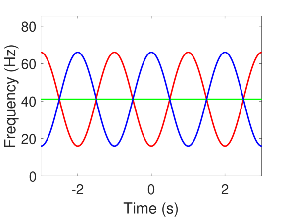
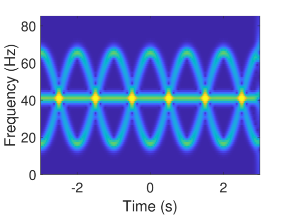
Figure 1: Micro-Doppler modulations induced by target’s tumbling (Left) and STFT of the signal (Right).

To be precise, we say that two signal components $x_{k}(t)$ and $x_{\ell}(t)$ of a multi-component signal $x(t)$ governed by (1) overlap in the time-frequency plane at $t=t_{0}$, if $\phi_{k}^{\prime}(t_{0})=\phi_{\ell}^{\prime}(t_{0})$ but $\phi_{k}^{\prime}(t)\not=\phi_{k}^{\prime}(t)$ in some deleted neighborhood of $t_{0}$. Based on the linear chirp-based model proposed in our previous paper [31], we have extended the SSO method in [12] by incorporating a chirp rate parameter to introduce a computational scheme in our work [32] for the recovery of signal components with overlapping frequency curves. In the present paper, we propose another innovative time-scale approach by introducing a 3D time-scale-chirp_rate transform, formulated by incorporating a complex quadratic phase function with a continuous wavelet-like transform (CWLT), to be called an adaptive “time-scale-chirp_rate (TSC-R)” component recovery operator, and develop a rigorous theory for assurance of solving the inverse problem in separating the signal components $x_{k}(t)$ of the multi-component signal $x(t)$ governed by (1), without the assumption of well separated IFs, but rather by assuming that if the two IF curves of the signal components $x_{k}$ and $x_{\ell}$ cross at some $t=t_{0}$, then $|\phi^{\prime\prime}_{k}(t)-\phi^{\prime\prime}_{\ell}(t)|\geq\delta$ for some $\delta>0$, for $|t-t_{0}|<\epsilon$, where $\epsilon>0$.

For convenience, we will consider, without loss of generality, the following complex-version of (1) without the trend function $A_{0}(t)$ function, namely:

$$x(t)=\sum_{k=1}^{K}x_{k}(t)=\sum_{k=1}^{K}A_{k}(t)e^{i2\pi\phi_{k}(t)}$$ (2)

where $A_{k}(t),\phi_{k}^{\prime}(t)>0$. The reader is referred to [12] for the methods of polynomial trend removal.

The presentation of this paper is organized as follows. In Section 2, the adaptive TSC-R operator is introduced and developed, along with some error bounds, for instantaneous frequency estimation and signal components recovery. When the Gaussian function is used as the wavelet-like scalable window, more precise error bounds are derived for the adaptive TSC-R operation in Section 3. Numerical experimental results will be discussed in Section 4.

2 Time-scale-chirp_rate signal recovery operator

To extract and separate the (unknown) signal components with crossover IFs from the multi-component signal governed by (2), we propose the following adaptive time-scale-chirp_rate signal recovery (TSC-R) operator, by introducing an adaptive continuous wavelet-like transform (CWLT), namely:

$$U_{x}(a,b,\lambda)\hskip-17.07182pt :=\int_{-\infty}^{\infty}x(t)\frac{1}{a}g\big{(}\frac{t-b}{a\sigma(b)}\big{)}e^{-i2\pi\mu\frac{t-b}{a}}e^{-i\pi\lambda(t-b)^{2}}dt$$ (3)

$$=\int_{{\mathbb{R}}}x(b+at)\frac{1}{\sigma(b)}g\big{(}\frac{t}{\sigma(b)}\big{)}e^{-i2\pi\mu t-i\pi\lambda a^{2}t^{2}}dt,$$

where $g(t)$ is a window function, $\mu$ is a positive constant, and $\sigma(b)$ is a positive function of $b$. In this paper, all window functions $g$ are assumed to be functions in $L_{2}({\mathbb{R}})$ that decay to zero at $\infty$ and satisfy $\int_{\mathbb{R}}g(t)dt=1$. Observe that when $\lambda=0$, $U_{x}(a,b,\lambda)$ is reduced to the adaptive CWLT of $x(t)$, denoted by $\widetilde{W}_{x}(a,b)$, as considered in [29], and that the TSC-R of $x(t)$ can be considered as a multi-component signal in the 3-dimensional space of time $t$, scale $a$, and chirp rate $\lambda$. The importance of this transform is that when the IF curves of two components $x_{k}(t)$ and $x_{\ell}(t)$ cross each other, they may be well-separated in the 3-dimensional space by adaptive TSC-R operator, provided that $\phi_{k}^{\prime\prime}(t)\not=\phi_{\ell}^{\prime\prime}(t)$ for $t$ in some neighborhood of the cross-over time instant $t_{0}$. Thus, a multi-component signal $x(t)$ with certain signal components that have the same IF values can be extracted and well-separated in the 3-dimensional TSC-R space adaptively. Hence, it is feasible to reconstruct signal components by adaptive TSC-R.

In practice, for a particular signal $x(t)$, its adaptive CWLT $\widetilde{W}_{x}(a,b)$ lies in a region of the scale-time plane:

$$\{(a,b):\;a_{1}(b)\leq a\leq a_{2}(b),b\in{\mathbb{R}}\}$$

for some $0<a_{1}(b),a_{2}(b)<\infty$. That is $\widetilde{W}_{x}(a,b)$ is negligible for $(a,b)$ outside this region. Throughout this paper we assume for each $b\in{\mathbb{R}}$, the scale $a$ is in the interval:

$$a_{1}(b)\leq a\leq a_{2}(b).$$ (4)

Definition 1.

For $\epsilon_{1}>0$ and $\epsilon_{3}>0$, let $\mathcal{E}_{\epsilon_{1},\epsilon_{3}}$ denote the set consisting of (complex) adaptive harmonic models (AHMs) defined by (2) with $A_{k}(t)\in L_{\infty}({\mathbb{R}}),\;A_{k}(t)>0,\phi_{k}(t)\in C^{3}({\mathbb{R}}),\inf_{b\in{\mathbb{R}}}\phi_{k}^{\prime}(t)>0,\sup_{b\in{\mathbb{R}}}\phi_{k}^{\prime}(t)<\infty$, and $A_{k}(t),\phi_{k}(t)$ satisfying

$$|A_{k}(t+\tau)-A_{k}(t)|\leq\varepsilon_{1}|\tau|A_{k}(t),~{}~{}t\in{\mathbb{R}},\;k=1,\cdots,K,$$ (5)

$$|\phi^{\prime\prime\prime}_{k}(t)|\leq\varepsilon_{3},~{}~{}t\in{\mathbb{R}},\;k=1,\cdots,K.$$ (6)

For a window function $g\in L_{1}({\mathbb{R}})$, denote

$$\mathchoice{\mathop{\vbox{\halign{#\cr\kern 0.80002pt$\hss\leavevmode\resizebox{4.10278pt}{3.8889pt}{\rotatebox[origin={c}]{90.0}{(}}\hss$\crcr\nointerlineskip\cr$\hss\displaystyle g\hss$\crcr}}}\limits}{\mathop{\vbox{\halign{#\cr\kern 0.80002pt$\hss\leavevmode\resizebox{4.10278pt}{3.8889pt}{\rotatebox[origin={c}]{90.0}{(}}\hss$\crcr\nointerlineskip\cr$\hss\textstyle g\hss$\crcr}}}\limits}{\mathop{\vbox{\halign{#\cr\kern 0.80002pt$\hss\leavevmode\resizebox{2.87193pt}{2.72223pt}{\rotatebox[origin={c}]{90.0}{(}}\hss$\crcr\nointerlineskip\cr$\hss\scriptstyle g\hss$\crcr}}}\limits}{\mathop{\vbox{\halign{#\cr\kern 0.80002pt$\hss\leavevmode\resizebox{2.05138pt}{1.94444pt}{\rotatebox[origin={c}]{90.0}{(}}\hss$\crcr\nointerlineskip\cr$\hss\scriptscriptstyle g\hss$\crcr}}}\limits}(\eta,\lambda):=\int_{{\mathbb{R}}}g(t)e^{-i2\pi\eta t-i\pi\lambda t^{2}}dt.$$ (7)

$\mathchoice{\mathop{\vbox{\halign{#\cr\kern 0.80002pt$\hss\leavevmode\resizebox{4.10278pt}{3.8889pt}{\rotatebox[origin={c}]{90.0}{(}}\hss$\crcr\nointerlineskip\cr$\hss\displaystyle g\hss$\crcr}}}\limits}{\mathop{\vbox{\halign{#\cr\kern 0.80002pt$\hss\leavevmode\resizebox{4.10278pt}{3.8889pt}{\rotatebox[origin={c}]{90.0}{(}}\hss$\crcr\nointerlineskip\cr$\hss\textstyle g\hss$\crcr}}}\limits}{\mathop{\vbox{\halign{#\cr\kern 0.80002pt$\hss\leavevmode\resizebox{2.87193pt}{2.72223pt}{\rotatebox[origin={c}]{90.0}{(}}\hss$\crcr\nointerlineskip\cr$\hss\scriptstyle g\hss$\crcr}}}\limits}{\mathop{\vbox{\halign{#\cr\kern 0.80002pt$\hss\leavevmode\resizebox{2.05138pt}{1.94444pt}{\rotatebox[origin={c}]{90.0}{(}}\hss$\crcr\nointerlineskip\cr$\hss\scriptscriptstyle g\hss$\crcr}}}\limits}(\eta,\lambda)$ is called a polynomial Fourier transform of $g$ [34, 44]. Note that $\mathchoice{\mathop{\vbox{\halign{#\cr\kern 0.80002pt$\hss\leavevmode\resizebox{4.10278pt}{3.8889pt}{\rotatebox[origin={c}]{90.0}{(}}\hss$\crcr\nointerlineskip\cr$\hss\displaystyle g\hss$\crcr}}}\limits}{\mathop{\vbox{\halign{#\cr\kern 0.80002pt$\hss\leavevmode\resizebox{4.10278pt}{3.8889pt}{\rotatebox[origin={c}]{90.0}{(}}\hss$\crcr\nointerlineskip\cr$\hss\textstyle g\hss$\crcr}}}\limits}{\mathop{\vbox{\halign{#\cr\kern 0.80002pt$\hss\leavevmode\resizebox{2.87193pt}{2.72223pt}{\rotatebox[origin={c}]{90.0}{(}}\hss$\crcr\nointerlineskip\cr$\hss\scriptstyle g\hss$\crcr}}}\limits}{\mathop{\vbox{\halign{#\cr\kern 0.80002pt$\hss\leavevmode\resizebox{2.05138pt}{1.94444pt}{\rotatebox[origin={c}]{90.0}{(}}\hss$\crcr\nointerlineskip\cr$\hss\scriptscriptstyle g\hss$\crcr}}}\limits}(0,0)=1$ since $\int_{\mathbb{R}}g(t)dt=1$.

When $g$ is the Gaussian function defined by

$$g(t)=\frac{1}{\sqrt{2\pi}}\;e^{-\frac{t^{2}}{2}},$$ (8)

then we have (refer to [19, 28])

$$\mathchoice{\mathop{\vbox{\halign{#\cr\kern 0.80002pt$\hss\leavevmode\resizebox{4.10278pt}{3.8889pt}{\rotatebox[origin={c}]{90.0}{(}}\hss$\crcr\nointerlineskip\cr$\hss\displaystyle g\hss$\crcr}}}\limits}{\mathop{\vbox{\halign{#\cr\kern 0.80002pt$\hss\leavevmode\resizebox{4.10278pt}{3.8889pt}{\rotatebox[origin={c}]{90.0}{(}}\hss$\crcr\nointerlineskip\cr$\hss\textstyle g\hss$\crcr}}}\limits}{\mathop{\vbox{\halign{#\cr\kern 0.80002pt$\hss\leavevmode\resizebox{2.87193pt}{2.72223pt}{\rotatebox[origin={c}]{90.0}{(}}\hss$\crcr\nointerlineskip\cr$\hss\scriptstyle g\hss$\crcr}}}\limits}{\mathop{\vbox{\halign{#\cr\kern 0.80002pt$\hss\leavevmode\resizebox{2.05138pt}{1.94444pt}{\rotatebox[origin={c}]{90.0}{(}}\hss$\crcr\nointerlineskip\cr$\hss\scriptscriptstyle g\hss$\crcr}}}\limits}(\eta,\lambda)=\frac{1}{\sqrt{1+i2\pi\lambda}}e^{-\frac{2\pi^{2}\eta^{2}}{1+i2\pi\lambda}},$$ (9)

where $\sqrt{1+i2\pi\lambda}$ denotes the square root of $1+i2\pi\lambda$ lying in the same quadrant as $1+i2\pi\lambda$.

We say $s(t)$ is a linear chirp or a linear frequency modulation signal if

$$s(t)=Ae^{i2\pi\phi(t)}=Ae^{i2\pi(ct+\frac{1}{2}rt^{2})},$$

where $c$ and $r$ are constants. We use linear chirps to approximate each $x_{k}(t)$ at any local time. Namely, we write

$$x_{k}(b+at)=x_{k}(b)e^{i2\pi(\phi^{\prime}_{k}(b)at+\frac{1}{2}\phi^{\prime\prime}_{k}(b)(at)^{2})}+x_{{\rm r},k}(a,b,t),$$

where

$$x_{{\rm r},k}(a,b,t)=x_{k}(b+at)-x_{k}(b)e^{i2\pi(\phi^{\prime}_{k}(b)at+\frac{1}{2}\phi^{\prime\prime}_{k}(b)(at)^{2})}.$$

Note that, as a function of $t$, $x_{k}(b)e^{i2\pi(\phi^{\prime}_{k}(b)at+\frac{1}{2}\phi^{\prime\prime}_{k}(b)a^{2}t^{2})}$ is a linear chirp. Thus $x(b+at)$ can be approximated by a superposition of linear chirps at any local time $t$:

$$x(b+at)=x_{\rm m}(a,b,t)+x_{\rm r}(a,b,t),$$

where

$$x_{\rm m}(a,b,t):=\sum_{k=1}^{K}x_{k}(b)e^{i2\pi(\phi_{k}^{\prime}(b)at+\frac{1}{2}\phi^{\prime\prime}_{k}(b)(at)^{2})}\;,$$

$$x_{\rm r}(a,b,t):=\sum_{k=1}^{K}x_{{\rm r},k}(a,b,t).$$

Denote

$$\mathfrak{R}_{x}(a,b,\lambda):=\int_{{\mathbb{R}}}x_{\rm m}(a,b,t)\frac{1}{\sigma(b)}g\big{(}\frac{t}{\sigma(b)}\big{)}e^{-i2\pi\mu t-i\pi\lambda a^{2}t^{2}}dt.$$ (10)

Then we have

$$\mathfrak{R}_{x}(a,b,\lambda)=\sum_{k=1}^{K}x_{k}(b)\mathchoice{\mathop{\vbox{\halign{#\cr\kern 0.80002pt$\hss\leavevmode\resizebox{4.10278pt}{3.8889pt}{\rotatebox[origin={c}]{90.0}{(}}\hss$\crcr\nointerlineskip\cr$\hss\displaystyle g\hss$\crcr}}}\limits}{\mathop{\vbox{\halign{#\cr\kern 0.80002pt$\hss\leavevmode\resizebox{4.10278pt}{3.8889pt}{\rotatebox[origin={c}]{90.0}{(}}\hss$\crcr\nointerlineskip\cr$\hss\textstyle g\hss$\crcr}}}\limits}{\mathop{\vbox{\halign{#\cr\kern 0.80002pt$\hss\leavevmode\resizebox{2.87193pt}{2.72223pt}{\rotatebox[origin={c}]{90.0}{(}}\hss$\crcr\nointerlineskip\cr$\hss\scriptstyle g\hss$\crcr}}}\limits}{\mathop{\vbox{\halign{#\cr\kern 0.80002pt$\hss\leavevmode\resizebox{2.05138pt}{1.94444pt}{\rotatebox[origin={c}]{90.0}{(}}\hss$\crcr\nointerlineskip\cr$\hss\scriptscriptstyle g\hss$\crcr}}}\limits}\Big{(}\sigma(b)\big{(}\mu-a\phi^{\prime}_{k}(b)\big{)},\sigma^{2}(b)a^{2}\big{(}\lambda-\phi^{\prime\prime}_{k}(b)\big{)}\Big{)}.$$ (11)

In the following, we denote

$$\nu=\nu(b):=\min_{1\leq k\leq K}A_{k}(b),~{}~{}M=M(b):=\sum_{k=1}^{K}A_{k}(b).$$ (12)

In the next lemma we provide an error bound for $|U_{x}(a,b,\lambda)-\mathfrak{R}_{x}(a,b,\lambda)|$.

Lemma 1.

Let $x(t)\in\mathcal{E}_{\epsilon_{1},\epsilon_{3}}$ for some $\epsilon_{1}>0,\epsilon_{3}>0$, and let $U_{x}(a,b,\lambda)$ be its adaptive TSC-R defined by (3) with a window function $g$ and $\mathfrak{R}_{x}(a,b,\lambda)$ the approximation of $U_{x}(a,b,\lambda)$ defined by (10). Then

$$\big{|}U_{x}(a,b,\lambda)-\mathfrak{R}_{x}(a,b,\lambda)\big{|}\leq M(b)\Pi(a,b),$$ (13)

where

$$\Pi(a,b):=\varepsilon_{1}I_{1}a\sigma(b)+\frac{\pi}{3}\varepsilon_{3}I_{3}a^{3}\sigma^{3}(b),$$ (14)

with

$$I_{n}:=\int_{\mathbb{R}}\big{|}g(t)t^{n}\big{|}dt,\;n=1,2,\cdots.$$ (15)

Proof.

By (5) and (6),

$$|x(b+at)-x_{\rm m}(a,b,t)|=|x_{\rm r}(a,b,t)|$$

$$=\sum_{k=1}^{K}\Big{\{}(A_{k}(b+at)-A_{k}(b))e^{i2\pi\phi_{k}(b+at)}$$

$$\hskip 28.45274pt+x_{k}(b)e^{i2\pi(\phi^{\prime}_{k}(b)at+\frac{1}{2}\phi^{\prime\prime}_{k}(b)(at)^{2})}\big{(}e^{i2\pi(\phi_{k}(b+at)-\phi_{k}(b)-\phi_{k}^{\prime}(b)at-\frac{1}{2}\phi^{\prime\prime}_{k}(b)(at)^{2})}-1\big{)}\Big{\}}$$

$$\leq\sum_{k=1}^{K}\Big{\{}\Big{|}A_{k}(b+at)-A_{k}(b)\Big{|}+A_{k}(b)\Big{|}i2\pi\Big{(}\phi_{k}(b+at)-\phi_{k}(b)-\phi_{k}^{\prime}(b)at-\frac{1}{2}\phi^{\prime\prime}_{k}(b)(at)^{2}\Big{)}\Big{|}\Big{\}}$$

$$\leq\sum_{k=1}^{K}\Big{\{}A_{k}(b)\varepsilon_{1}a|t|+A_{k}(b)2\pi\sup_{\xi\in{\mathbb{R}}}\frac{1}{6}\big{|}\phi^{\prime\prime\prime}_{k}(\xi)(at)^{3}\big{|}\Big{\}}$$

$$\leq M(b)\varepsilon_{1}a|t|+M(b)\frac{\pi}{3}\varepsilon_{3}a^{3}|t|^{3}.$$

This leads to

$$\big{|}U_{x}(a,b,\lambda)-\mathfrak{R}_{x}(a,b,\lambda)\big{|}=\Big{|}\int_{\mathbb{R}}(x(b+at)-x_{\rm m}(a,b,t))\frac{1}{\sigma(b)}g(\frac{t}{\sigma(b)})e^{-i2\pi\mu at-i\pi\lambda(at)^{2}}dt\Big{|}$$

$$\qquad\leq\int_{\mathbb{R}}M(b)\big{(}\varepsilon_{1}a|t|+\frac{\pi}{3}\varepsilon_{3}a^{3}|t|^{3}\big{)}\big{|}\frac{1}{\sigma(b)}g(\frac{t}{\sigma(b)})\big{|}dt$$

$$\qquad=M(b)\big{(}\varepsilon_{1}I_{1}\sigma(b)+\frac{\pi}{3}\varepsilon_{3}I_{3}\sigma^{3}(b)\big{)}.$$

This completes the proof of Lemma 1. ∎

Remark 1.

Recall that we assume in this paper $a$ is in an interval as shown in (4). Thus, we have

$$\big{|}U_{x}(a,b,\lambda)-\mathfrak{R}_{x}(a,b,\lambda)\big{|}\leq M(b)\Pi_{0}(b),$$ (16)

where

$$\Pi_{0}(b):=\Pi(a_{2},b)=\varepsilon_{1}I_{1}\sigma(b)a_{2}+\frac{\pi}{3}\varepsilon_{3}I_{3}\sigma^{3}(b)a_{2}^{3}.$$ (17)

$\blacksquare$

In the following, we assume any two IF curves of the signal components $x_{k}$ and $x_{\ell}$ satsify

$$\hbox{either}~{}~{}\frac{|\phi^{\prime}_{k}(t)-\phi^{\prime}_{\ell}(t)|}{\phi^{\prime}_{k}(t)+\phi^{\prime}_{\ell}(t)}\geq\triangle,\;t\in{\mathbb{R}},~{}~{}\hbox{or}~{}~{}|\phi^{\prime\prime}_{k}(t)-\phi^{\prime\prime}_{\ell}(t)|\geq 2\triangle_{1},\;t\in{\mathbb{R}},$$ (18)

where $0<\triangle<1,\triangle_{1}>0$. Clearly $\phi^{\prime}_{k}(t)$ and $\phi^{\prime}_{\ell}(t)$ could be cross over at a time instant. For $1\leq k\leq K$, define

$$Z_{k}:=\{(a,b,\lambda):\;|\mu-a\phi^{\prime}_{k}(b)|<\triangle~{}\hbox{and}~{}|\lambda-\phi^{\prime\prime}_{k}(b)|<\triangle_{1},\;b\in{\mathbb{R}}\}.$$ (19)

Lemma 2.

If $\phi_{k}$ satisfies (18), then $Z_{k},1\leq k\leq K$ are disjoint, that is $Z_{\ell}\cap Z_{k}=\emptyset$ for $\ell\not=k$.

The proof of Lemma 2 is straightforward and it is omitted.

Note that for $(a,b,\lambda)\in Z_{\ell}$, the scale variable $a$ satisfies

$$\frac{\mu-\triangle}{\phi^{\prime}_{\ell}(b)}<a<\frac{\mu+\triangle}{\phi^{\prime}_{\ell}(b)}.$$

Hence for any $(a,b,\lambda)\in Z_{\ell}$, by (13), we have

$$\big{|}U_{x}(a,b,\lambda)-\mathfrak{R}_{x}(a,b,\lambda)\big{|}\leq M(b)\Pi_{\ell}(b),$$ (20)

where

$$\Pi_{\ell}(b):=\Pi(\frac{\mu+\triangle}{\phi^{\prime}_{\ell}(b)},b)=\varepsilon_{1}I_{1}\sigma(b)\frac{\mu+\triangle}{\phi^{\prime}_{\ell}(b)}+\frac{\pi}{3}\varepsilon_{3}I_{3}\sigma^{3}(b)\Big{(}\frac{\mu+\triangle}{\phi^{\prime}_{\ell}(b)}\Big{)}^{3}.$$ (21)

For a fixed $b$, and a positive number $\widetilde{\epsilon}_{1}$, we let $\mathcal{H}_{b}$ and $\mathcal{H}_{b,k}$ denote the sets defined by

$$\begin{array}[]{l}\mathcal{H}_{b}:=\big{\{}(a,\lambda):\;|U_{x}(a,b,\lambda)|>\widetilde{\epsilon}_{1}\big{\}},\\ \mathcal{H}_{b,k}:=\Big{\{}(a,\lambda)\in\mathcal{H}_{b}:\;|\mu-a\phi^{\prime}_{k}(b)|<\triangle~{}\hbox{and}~{}|\lambda-\phi^{\prime\prime}_{k}(b)|<\triangle_{1}\Big{\}}.\end{array}$$ (22)

Note that $\mathcal{H}_{b}$ and $\mathcal{H}_{b,k}$ depend on $\widetilde{\epsilon}_{1}$, and for simplicity of presentation, we drop $\widetilde{\epsilon}_{1}$ from them.

Let $\Upsilon(b),\Upsilon_{\ell,k}(b)$ with $\Upsilon(b)\geq\Upsilon_{\ell,k}(b)$ for $k\not=\ell$ be some functions satisfying

$$\begin{array}[]{l}\sup_{\{(a,\lambda):(a,b,\lambda)\not\in\cup_{k=1}^{K}Z_{k}\}}\big{|}\mathchoice{\mathop{\vbox{\halign{#\cr\kern 0.80002pt$\hss\leavevmode\resizebox{4.10278pt}{3.8889pt}{\rotatebox[origin={c}]{90.0}{(}}\hss$\crcr\nointerlineskip\cr$\hss\displaystyle g\hss$\crcr}}}\limits}{\mathop{\vbox{\halign{#\cr\kern 0.80002pt$\hss\leavevmode\resizebox{4.10278pt}{3.8889pt}{\rotatebox[origin={c}]{90.0}{(}}\hss$\crcr\nointerlineskip\cr$\hss\textstyle g\hss$\crcr}}}\limits}{\mathop{\vbox{\halign{#\cr\kern 0.80002pt$\hss\leavevmode\resizebox{2.87193pt}{2.72223pt}{\rotatebox[origin={c}]{90.0}{(}}\hss$\crcr\nointerlineskip\cr$\hss\scriptstyle g\hss$\crcr}}}\limits}{\mathop{\vbox{\halign{#\cr\kern 0.80002pt$\hss\leavevmode\resizebox{2.05138pt}{1.94444pt}{\rotatebox[origin={c}]{90.0}{(}}\hss$\crcr\nointerlineskip\cr$\hss\scriptscriptstyle g\hss$\crcr}}}\limits}\big{(}\sigma(b)(\mu-a\phi^{\prime}_{k}(b)),\sigma^{2}(b)a^{2}(\lambda-\phi^{\prime\prime}_{k}(b))\big{)}\big{|}\leq\Upsilon(b),\\ \sup_{\{(a,\lambda):(a,b,\lambda)\not\in Z_{\ell}\}}\big{|}\mathchoice{\mathop{\vbox{\halign{#\cr\kern 0.80002pt$\hss\leavevmode\resizebox{4.10278pt}{3.8889pt}{\rotatebox[origin={c}]{90.0}{(}}\hss$\crcr\nointerlineskip\cr$\hss\displaystyle g\hss$\crcr}}}\limits}{\mathop{\vbox{\halign{#\cr\kern 0.80002pt$\hss\leavevmode\resizebox{4.10278pt}{3.8889pt}{\rotatebox[origin={c}]{90.0}{(}}\hss$\crcr\nointerlineskip\cr$\hss\textstyle g\hss$\crcr}}}\limits}{\mathop{\vbox{\halign{#\cr\kern 0.80002pt$\hss\leavevmode\resizebox{2.87193pt}{2.72223pt}{\rotatebox[origin={c}]{90.0}{(}}\hss$\crcr\nointerlineskip\cr$\hss\scriptstyle g\hss$\crcr}}}\limits}{\mathop{\vbox{\halign{#\cr\kern 0.80002pt$\hss\leavevmode\resizebox{2.05138pt}{1.94444pt}{\rotatebox[origin={c}]{90.0}{(}}\hss$\crcr\nointerlineskip\cr$\hss\scriptscriptstyle g\hss$\crcr}}}\limits}\big{(}\sigma(b)(\mu-a\phi^{\prime}_{k}(b)),\sigma^{2}(b)a^{2}(\lambda-\phi^{\prime\prime}_{k}(b))\big{)}\big{|}\leq\Upsilon_{\ell,k}(b).\end{array}$$ (23)

About the quantities $\Upsilon(b)$ and $\Upsilon_{\ell,k}(b)$, refer to Section 3 when $g$ is the Gaussian window function.

Next we provide another lemma which will be used to derive our main theorem. In the following lemma and the rest of this paper, $\sum_{k\not=\ell}$ denotes $\sum_{\{k:~{}k\not=\ell,1\leq k\leq K\}}$.

Lemma 3.

Let $x(t)\in\mathcal{E}_{\epsilon_{1},\epsilon_{3}}$ for some $\epsilon_{1}>0,\epsilon_{3}>0$, and $U_{x}(a,b,\lambda)$ be the adaptive TSC-R of $x(t)$ with a window function $g$. Then for any $(a,\lambda)\in\mathcal{H}_{b,\ell}$,

$$\big{|}U_{x}(a,b,\lambda)-x_{\ell}(b)\mathchoice{\mathop{\vbox{\halign{#\cr\kern 0.80002pt$\hss\leavevmode\resizebox{4.10278pt}{3.8889pt}{\rotatebox[origin={c}]{90.0}{(}}\hss$\crcr\nointerlineskip\cr$\hss\displaystyle g\hss$\crcr}}}\limits}{\mathop{\vbox{\halign{#\cr\kern 0.80002pt$\hss\leavevmode\resizebox{4.10278pt}{3.8889pt}{\rotatebox[origin={c}]{90.0}{(}}\hss$\crcr\nointerlineskip\cr$\hss\textstyle g\hss$\crcr}}}\limits}{\mathop{\vbox{\halign{#\cr\kern 0.80002pt$\hss\leavevmode\resizebox{2.87193pt}{2.72223pt}{\rotatebox[origin={c}]{90.0}{(}}\hss$\crcr\nointerlineskip\cr$\hss\scriptstyle g\hss$\crcr}}}\limits}{\mathop{\vbox{\halign{#\cr\kern 0.80002pt$\hss\leavevmode\resizebox{2.05138pt}{1.94444pt}{\rotatebox[origin={c}]{90.0}{(}}\hss$\crcr\nointerlineskip\cr$\hss\scriptscriptstyle g\hss$\crcr}}}\limits}\big{(}\sigma(b)(\mu-a\phi^{\prime}_{\ell}(b)),\sigma^{2}(b)a^{2}(\lambda-\phi^{\prime\prime}_{\ell}(b))\big{)}\big{|}\leq{\rm Err}_{\ell}(b),$$ (32)

where

$${\rm Err}_{\ell}(b):=M(b)\Pi_{\ell}(b)+\sum_{k\not=\ell}A_{k}(b)\Upsilon_{\ell,k}(b)$$ (33)

with $\Pi_{\ell}(b)$ defined by (21).

Proof.

By (11), we have for any $(a,\lambda)\in\mathcal{H}_{b,\ell}$,

$$\big{|}\mathfrak{R}_{x}(a,b,\lambda)-x_{\ell}(b)\mathchoice{\mathop{\vbox{\halign{#\cr\kern 0.80002pt$\hss\leavevmode\resizebox{4.10278pt}{3.8889pt}{\rotatebox[origin={c}]{90.0}{(}}\hss$\crcr\nointerlineskip\cr$\hss\displaystyle g\hss$\crcr}}}\limits}{\mathop{\vbox{\halign{#\cr\kern 0.80002pt$\hss\leavevmode\resizebox{4.10278pt}{3.8889pt}{\rotatebox[origin={c}]{90.0}{(}}\hss$\crcr\nointerlineskip\cr$\hss\textstyle g\hss$\crcr}}}\limits}{\mathop{\vbox{\halign{#\cr\kern 0.80002pt$\hss\leavevmode\resizebox{2.87193pt}{2.72223pt}{\rotatebox[origin={c}]{90.0}{(}}\hss$\crcr\nointerlineskip\cr$\hss\scriptstyle g\hss$\crcr}}}\limits}{\mathop{\vbox{\halign{#\cr\kern 0.80002pt$\hss\leavevmode\resizebox{2.05138pt}{1.94444pt}{\rotatebox[origin={c}]{90.0}{(}}\hss$\crcr\nointerlineskip\cr$\hss\scriptscriptstyle g\hss$\crcr}}}\limits}\big{(}\sigma(b)(\mu-a\phi^{\prime}_{\ell}(b)),\sigma^{2}(b)a^{2}(\lambda-\phi^{\prime\prime}_{\ell}(b))\big{)}\big{|}$$

$$=\Big{|}\sum_{k\not=\ell}x_{k}(b)\mathchoice{\mathop{\vbox{\halign{#\cr\kern 0.80002pt$\hss\leavevmode\resizebox{4.10278pt}{3.8889pt}{\rotatebox[origin={c}]{90.0}{(}}\hss$\crcr\nointerlineskip\cr$\hss\displaystyle g\hss$\crcr}}}\limits}{\mathop{\vbox{\halign{#\cr\kern 0.80002pt$\hss\leavevmode\resizebox{4.10278pt}{3.8889pt}{\rotatebox[origin={c}]{90.0}{(}}\hss$\crcr\nointerlineskip\cr$\hss\textstyle g\hss$\crcr}}}\limits}{\mathop{\vbox{\halign{#\cr\kern 0.80002pt$\hss\leavevmode\resizebox{2.87193pt}{2.72223pt}{\rotatebox[origin={c}]{90.0}{(}}\hss$\crcr\nointerlineskip\cr$\hss\scriptstyle g\hss$\crcr}}}\limits}{\mathop{\vbox{\halign{#\cr\kern 0.80002pt$\hss\leavevmode\resizebox{2.05138pt}{1.94444pt}{\rotatebox[origin={c}]{90.0}{(}}\hss$\crcr\nointerlineskip\cr$\hss\scriptscriptstyle g\hss$\crcr}}}\limits}\big{(}\sigma(b)(\mu-a\phi^{\prime}_{k}(b)),\sigma^{2}(b)a^{2}(\lambda-\phi^{\prime\prime}_{k}(b))\big{)}\Big{|}$$

$$\leq\sum_{k\not=\ell}A_{k}(b)\Big{|}\mathchoice{\mathop{\vbox{\halign{#\cr\kern 0.80002pt$\hss\leavevmode\resizebox{4.10278pt}{3.8889pt}{\rotatebox[origin={c}]{90.0}{(}}\hss$\crcr\nointerlineskip\cr$\hss\displaystyle g\hss$\crcr}}}\limits}{\mathop{\vbox{\halign{#\cr\kern 0.80002pt$\hss\leavevmode\resizebox{4.10278pt}{3.8889pt}{\rotatebox[origin={c}]{90.0}{(}}\hss$\crcr\nointerlineskip\cr$\hss\textstyle g\hss$\crcr}}}\limits}{\mathop{\vbox{\halign{#\cr\kern 0.80002pt$\hss\leavevmode\resizebox{2.87193pt}{2.72223pt}{\rotatebox[origin={c}]{90.0}{(}}\hss$\crcr\nointerlineskip\cr$\hss\scriptstyle g\hss$\crcr}}}\limits}{\mathop{\vbox{\halign{#\cr\kern 0.80002pt$\hss\leavevmode\resizebox{2.05138pt}{1.94444pt}{\rotatebox[origin={c}]{90.0}{(}}\hss$\crcr\nointerlineskip\cr$\hss\scriptscriptstyle g\hss$\crcr}}}\limits}\big{(}\sigma(b)(\mu-a\phi^{\prime}_{k}(b)),\sigma^{2}(b)a^{2}(\lambda-\phi^{\prime\prime}_{k}(b))\big{)}\Big{|}\leq\sum_{k\not=\ell}A_{k}(b)\Upsilon_{\ell,k}(b).$$

This, along with (20), leads to that

Left hand side of (32)

$$\leq\big{|}U_{x}(a,b,\lambda)-\mathfrak{R}_{x}(a,b,\lambda)\big{|}+\big{|}\mathfrak{R}_{x}(a,b,\lambda)-x_{\ell}(b)\mathchoice{\mathop{\vbox{\halign{#\cr\kern 0.80002pt$\hss\leavevmode\resizebox{4.10278pt}{3.8889pt}{\rotatebox[origin={c}]{90.0}{(}}\hss$\crcr\nointerlineskip\cr$\hss\displaystyle g\hss$\crcr}}}\limits}{\mathop{\vbox{\halign{#\cr\kern 0.80002pt$\hss\leavevmode\resizebox{4.10278pt}{3.8889pt}{\rotatebox[origin={c}]{90.0}{(}}\hss$\crcr\nointerlineskip\cr$\hss\textstyle g\hss$\crcr}}}\limits}{\mathop{\vbox{\halign{#\cr\kern 0.80002pt$\hss\leavevmode\resizebox{2.87193pt}{2.72223pt}{\rotatebox[origin={c}]{90.0}{(}}\hss$\crcr\nointerlineskip\cr$\hss\scriptstyle g\hss$\crcr}}}\limits}{\mathop{\vbox{\halign{#\cr\kern 0.80002pt$\hss\leavevmode\resizebox{2.05138pt}{1.94444pt}{\rotatebox[origin={c}]{90.0}{(}}\hss$\crcr\nointerlineskip\cr$\hss\scriptscriptstyle g\hss$\crcr}}}\limits}\big{(}\sigma(b)(\mu-a\phi^{\prime}_{\ell}(b)),\sigma^{2}(b)a^{2}(\lambda-\phi^{\prime\prime}_{\ell}(b))\big{)}\big{|}$$

$$\leq M(b)\Pi_{\ell}(b)+\sum_{k\not=\ell}A_{k}(b)\Upsilon_{\ell,k}(b).$$

Thus (32) holds true. ∎

Next we have the following theorem.

Theorem 1.

Let $x(t)\in\mathcal{E}_{\epsilon_{1},\epsilon_{3}}$ for some $\epsilon_{1}>0,\epsilon_{3}>0$, and $U_{x}(a,b,\lambda)$ be the adaptive TSC-R of $x(t)$ with a window function $g$. Suppose $x(t)$ satisfies (18) for some $0<\triangle<1$ and $\triangle_{1}>0$, and

$$2M(b)\big{(}\Upsilon(b)+\Pi_{0}(b)\big{)}\leq\nu(b)$$ (38)

holds. Let $\mathcal{H}_{b}$ and $\mathcal{H}_{b,k}$ be the sets defined by (22) with a function $\widetilde{\epsilon}_{1}=\widetilde{\epsilon}_{1}(b)>0$ satisfying

$$M(b)\big{(}\Upsilon(b)+\Pi_{0}(b)\big{)}\leq\widetilde{\epsilon}_{1}\leq\nu(b)-M(b)\big{(}\Upsilon(b)+\Pi_{0}(b)\big{)}.$$ (39)

Then the following statements hold.

1. $\mathcal{H}_{b}=\cup_{k=1}^{K}\mathcal{H}_{b,k}$.

2. The sets $\mathcal{H}_{b,k},1\leq k\leq K$ are disjoint, i.e. $\mathcal{H}_{b,k}\cap{\mathcal{H}}_{b,k^{\prime}{}}=\emptyset$ if $k\not=k^{\prime}{}$.

3. Each set $\mathcal{H}_{b,k}$ is non-empty.

We delay the proof of Theorem 1 to the end of this section.

Denote

$$(\widehat{a}_{\ell},\widehat{\lambda}_{\ell})=(\widehat{a}_{\ell}(b),\widehat{\lambda}_{\ell}(b)):={\rm argmax}_{(a,\lambda)\in\mathcal{H}_{b,\ell}}|U_{x}(a,b,\lambda)|,~{}~{}\ell=1,\cdots,K.$$ (40)

From Theorem 1, we know $\widehat{a}_{\ell}(b)$ and $\widehat{\lambda}_{\ell}(b)$ are well defined. We will use them to estimate $\phi^{\prime}_{\ell}(b)$, chirp rate $\phi^{{\prime}{\prime}}_{\ell}(b)$ and to recover $x_{\ell}(b)$. More precisely, we have the following TSC_R operator scheme for IF estimation and component recovery.

Algorithm 1.

(Time-Scale-Chirp_rate operator scheme)   Suppose $x(t)\in\mathcal{E}_{\epsilon_{1},\epsilon_{3}}$ satisfies the conditions in Theorem 1.

• Step 1. Calculate $\widehat{a}_{\ell}(b)$ and $\widehat{\lambda}_{\ell}(b)$ by (40).

• Step 2. Obtain IF and chirp rate estimates by

  $$\phi^{\prime}_{\ell}(b)\approx\frac{\mu}{\widehat{a}_{\ell}(b)},\quad\phi^{{\prime}{\prime}}_{\ell}(b)\approx\widehat{\lambda}_{\ell}(b),$$ (41)

• Step 3. Obtain the recovered $\ell$-th component by

  $$x_{\ell}(b)\approx U_{x}(\widehat{a}_{\ell},b,\widehat{\lambda}_{\ell}).$$ (42)

  $\blacksquare$

Observe that the recovered component is obtained simply by substituting the time-scale ridge $\widehat{a}_{\ell}(b)$ and time-chirp rate ridge $\widehat{\lambda}_{\ell}(b)$ to adaptive TSC-R, which is different from SST method with which the recovered $x_{k}(t)$ is computed by a definite integral along each estimated IF curve on the SST plane.

Next we study the error bounds for these approximations. To this regard, we introduce admissible window functions.

Definition 2.

(Admissible window function)   A function $g(t)$ in $L_{2}({\mathbb{R}})$ is called an admissible window function if $\int_{\mathbb{R}}g(t)dt=1$, $g$ has certain at $\infty$ and satisfies the following conditions.

• $|\mathchoice{\mathop{\vbox{\halign{#\cr\kern 0.80002pt$\hss\leavevmode\resizebox{4.10278pt}{3.8889pt}{\rotatebox[origin={c}]{90.0}{(}}\hss$\crcr\nointerlineskip\cr$\hss\displaystyle g\hss$\crcr}}}\limits}{\mathop{\vbox{\halign{#\cr\kern 0.80002pt$\hss\leavevmode\resizebox{4.10278pt}{3.8889pt}{\rotatebox[origin={c}]{90.0}{(}}\hss$\crcr\nointerlineskip\cr$\hss\textstyle g\hss$\crcr}}}\limits}{\mathop{\vbox{\halign{#\cr\kern 0.80002pt$\hss\leavevmode\resizebox{2.87193pt}{2.72223pt}{\rotatebox[origin={c}]{90.0}{(}}\hss$\crcr\nointerlineskip\cr$\hss\scriptstyle g\hss$\crcr}}}\limits}{\mathop{\vbox{\halign{#\cr\kern 0.80002pt$\hss\leavevmode\resizebox{2.05138pt}{1.94444pt}{\rotatebox[origin={c}]{90.0}{(}}\hss$\crcr\nointerlineskip\cr$\hss\scriptscriptstyle g\hss$\crcr}}}\limits}(\eta,\lambda)|$ can be written as $f(|\eta|,|\lambda|)$ for some function $f(\xi_{1},\xi_{2})$ defined on $0\leq\xi_{1},\xi_{2}<\infty$.

• There exist $c_{0}$ with $0<c_{0}<1$ and (strictly) decreasing non-negative continuous functions $\beta(\xi)$ and $\gamma(\xi)$ on $[0,\infty)$ with $\beta(0)=1$, $\gamma(0)=1$ such that if $f$ in (a) satisfies

  $$1-c\leq f(\eta,\lambda),$$ (43)

  for some $c$ with $0\leq c\leq c_{0}$ and $\eta,\lambda$, then

  $$1-c\leq\beta(\eta),\quad 1-c\leq\gamma(\lambda).$$ (44)

Theorem 2.

Let $x(t)\in\mathcal{E}_{\epsilon_{1},\epsilon_{3}}$ for some $\epsilon_{1}>0,\epsilon_{3}>0$, and $U_{x}(a,b,\lambda)$ be the adaptive TSC-R of $x(t)$ with an admissible window function $g$ for certain $c_{0}$ such that (44) holds. Suppose (18) and (38) hold and that for $1\leq\ell\leq K$, $2{\rm Err}_{\ell}(b)/A_{\ell}(b)\leq c_{0}$, where ${\rm Err}_{\ell}(b)$ is defined by (33). Let $\mathcal{H}_{b}$ and $\mathcal{H}_{b,k}$ be the sets defined by (22) for some $\widetilde{\epsilon}_{1}$ satisfying (39). Let $\widehat{a}_{\ell}(b),\widehat{\lambda}_{\ell}(b)$ be the functions defined by (40). Then the following statements hold.

1. For $\ell=1,2,\cdots,K$,

   $$|\mu-\widehat{a}_{\ell}(b)\phi_{\ell}^{\prime}(b)|\leq{\rm Bd}_{1,\ell}:=\frac{1}{\sigma(b)}\beta^{-1}\big{(}1-\frac{2\;{\rm Err}_{\ell}(b)}{A_{\ell}(b)}\big{)},$$ (45)

   $$|\widehat{\lambda}_{\ell}(b)-\phi_{\ell}^{\prime\prime}(b)|\leq{\rm Bd}_{2,\ell}:=\frac{1}{\sigma^{2}(b)\widehat{a}_{\ell}^{2}}\gamma^{-1}\big{(}1-\frac{2\;{\rm Err}_{\ell}(b)}{A_{\ell}(b)}\big{)}.$$ (46)

2. For $\ell=1,2,\cdots,K$,

   $$\big{|}U_{x}(\widehat{a}_{\ell},b,\widehat{\lambda}_{\ell})-x_{\ell}(b)\big{|}\leq{\rm Bd}_{3,\ell},$$ (47)

   where

   $${\rm Bd}_{3,\ell}:={\rm Err}_{\ell}(b)+2\pi I_{1}A_{\ell}(b)\beta^{-1}\big{(}1-\frac{2\;{\rm Err}_{\ell}(b)}{A_{\ell}(b)}\big{)}+\pi I_{2}A_{\ell}(b)\gamma^{-1}\big{(}1-\frac{2\;{\rm Err}_{\ell}(b)}{A_{\ell}(b)}\big{)}$$

   with $I_{1}$ and $I_{2}$ defined by (15).

3. If, in addition, the window function $g(t)\geq 0$ for $t\in{\mathbb{R}}$, then for $\ell=1,2,\cdots,K$,

   $$\big{|}|U_{x}(\widehat{a}_{\ell},b,\widehat{\lambda}_{\ell})|-A_{\ell}(b)\big{|}\leq{\rm Err}_{\ell}(b).$$ (48)

Note that since $\lim_{\xi\to 1^{-}}\beta^{-1}(\xi)=0$ and $\lim_{\xi\to 1^{-}}\gamma^{-1}(\xi)=0$, the error bounds ${\rm Bd}_{1,\ell}$, ${\rm Bd}_{2,\ell}$, ${\rm Bd}_{3,\ell}$ are small as long as ${\rm Err}_{\ell}(b)$ is small. We will study these error bounds in more details in the next section when $g$ is the Gaussian window function.

As shown in (45)-(48), $\frac{\mu}{\widehat{a}_{\ell}(b)}$ is an estimate to $\phi^{\prime}_{\ell}(b)$ as shown in (41) and $U_{x}(\widehat{a}_{\ell},b,\widehat{\lambda}_{\ell})$ is the recovered component of $x_{\ell}(b)$. For a real-valued $x_{\ell}(t)$, we will use

$$x_{\ell}(b)\approx 2{\rm Re}\Big{(}U_{x}(\widehat{a}_{\ell},b,\widehat{\lambda}_{\ell})\Big{)}.$$ (49)

In addition, the chirp rate $\phi^{{\prime}{\prime}}_{\ell}(b)$ and IA $A_{\ell}(b)$ can be estimated by $\widehat{\lambda}_{\ell}(b)$ and $|U_{x}(\widehat{a}_{\ell},b,\widehat{\lambda}_{\ell})|$ respectively.

Remark 2.

Adaptive TSC-R defined by (3) can be extended to adaptive CWLT with a higher order polynomial phase function. More precisely, one may define

$$U_{x}(a,b,\lambda_{1},\cdots,\lambda_{m})\hskip-17.07182pt :=\int_{-\infty}^{\infty}x(t)\frac{1}{a}\overline{\psi_{\sigma(b)}\big{(}\frac{t-b}{a}\big{)}}e^{-i2\pi\sum_{\ell=2}^{m+1}\lambda_{\ell-1}\frac{(t-b)^{\ell}}{\ell!}}dt$$ (50)

$$=\int_{{\mathbb{R}}}x(b+at)\frac{1}{\sigma(b)}g\big{(}\frac{t}{\sigma(b)}\big{)}e^{-i2\pi\mu t-i2\pi\sum_{\ell=2}^{m+1}\lambda_{\ell-1}\frac{(at)^{\ell}}{\ell!}}dt.$$

$U_{x}(a,b,\lambda_{1},\cdots,\lambda_{m})$ can be used for IF estimation and mode recovery of such a multicomponent signal that IFs $\phi^{{\prime}}_{k}(t)$ and $\phi^{{\prime}}_{\ell}(t)$ of two components are “highly” crossover at some time $t_{0}$: $\phi^{(j)}_{k}(t_{0})=\phi^{(j)}_{\ell}(t_{0}),1\leq j\leq m$. One can establish theorems similar Theorems 1 and 2 for $U_{x}(a,b,\lambda_{1},\cdots,\lambda_{m})$. $\blacksquare$

Finally in this section we present the proofs of Theorems 1 and 2. For simplicity of presentation, we write $\sigma$ for $\sigma(b)$.

Proof of Theorem 1(a). Clearly $\cup_{k=1}^{K}\mathcal{H}_{b,k}\subseteq\mathcal{H}_{b}$. Next we show $\mathcal{H}_{b}\subseteq\cup_{k=1}^{K}\mathcal{H}_{b,k}$.

Let $(a,\lambda)\in\mathcal{H}_{b}$. Suppose $(a,\lambda)\not\in\mathcal{H}_{b,k}$ for any $k$. Then $(a,b,\lambda)\not\in\cup_{k=1}^{K}Z_{k}$. Hence, by (23), we have

$$\big{|}\mathfrak{R}_{x}(a,b,\lambda)\big{|}\hskip-17.07182pt =\Big{|}\sum_{k=1}^{K}x_{k}(b)\mathchoice{\mathop{\vbox{\halign{#\cr\kern 0.80002pt$\hss\leavevmode\resizebox{4.10278pt}{3.8889pt}{\rotatebox[origin={c}]{90.0}{(}}\hss$\crcr\nointerlineskip\cr$\hss\displaystyle g\hss$\crcr}}}\limits}{\mathop{\vbox{\halign{#\cr\kern 0.80002pt$\hss\leavevmode\resizebox{4.10278pt}{3.8889pt}{\rotatebox[origin={c}]{90.0}{(}}\hss$\crcr\nointerlineskip\cr$\hss\textstyle g\hss$\crcr}}}\limits}{\mathop{\vbox{\halign{#\cr\kern 0.80002pt$\hss\leavevmode\resizebox{2.87193pt}{2.72223pt}{\rotatebox[origin={c}]{90.0}{(}}\hss$\crcr\nointerlineskip\cr$\hss\scriptstyle g\hss$\crcr}}}\limits}{\mathop{\vbox{\halign{#\cr\kern 0.80002pt$\hss\leavevmode\resizebox{2.05138pt}{1.94444pt}{\rotatebox[origin={c}]{90.0}{(}}\hss$\crcr\nointerlineskip\cr$\hss\scriptscriptstyle g\hss$\crcr}}}\limits}\big{(}\sigma(\mu-a\phi^{\prime}_{k}(b)),\sigma^{2}a^{2}(\lambda-\phi^{\prime\prime}_{k}(b))\big{)}\Big{|}$$

$$\leq\sum_{k=1}^{K}A_{k}(b)\Upsilon(b)=M(b)\Upsilon(b).$$

This, together with (16), implies

$$\big{|}U_{x}(a,b,\lambda)\big{|}\hskip-17.07182pt \leq\big{|}U_{x}(a,b,\lambda)-\mathfrak{R}_{x}(a,b,\lambda)\big{|}+\big{|}\mathfrak{R}_{x}(a,b,\lambda)\big{|}$$

$$\leq M(b)\Pi_{0}(b)+M(b)\Upsilon(b)\leq\widetilde{\epsilon}_{1},$$

a contradiction to that $(a,\lambda)\in\mathcal{H}_{b}$. Hence there must exist an $\ell$ such that $(a,\lambda)\in\mathcal{H}_{b,\ell}$. This shows $\mathcal{H}_{b}=\cup_{k=1}^{K}\mathcal{H}_{b,k}$.

Proof of Theorem 1(b). Observe that $\mathcal{H}_{b,k}=\mathcal{H}_{b}\cap\{(a,\lambda):(a,b,\lambda)\in Z_{k}\}$. Since $Z_{k},1\leq k\leq K$ are disjoint, we conclude that $\mathcal{H}_{b,k},1\leq k\leq K$ are also disjoint.

Proof of Theorem 1(c). To show that each $\mathcal{H}_{b,\ell}$ is non-empty, it is enough to show $(\frac{\mu}{\phi^{\prime}_{\ell}(b)},\phi^{\prime\prime}_{\ell}(b))\in\mathcal{H}_{b}$. Indeed, with $\mathchoice{\mathop{\vbox{\halign{#\cr\kern 0.80002pt$\hss\leavevmode\resizebox{4.10278pt}{3.8889pt}{\rotatebox[origin={c}]{90.0}{(}}\hss$\crcr\nointerlineskip\cr$\hss\displaystyle g\hss$\crcr}}}\limits}{\mathop{\vbox{\halign{#\cr\kern 0.80002pt$\hss\leavevmode\resizebox{4.10278pt}{3.8889pt}{\rotatebox[origin={c}]{90.0}{(}}\hss$\crcr\nointerlineskip\cr$\hss\textstyle g\hss$\crcr}}}\limits}{\mathop{\vbox{\halign{#\cr\kern 0.80002pt$\hss\leavevmode\resizebox{2.87193pt}{2.72223pt}{\rotatebox[origin={c}]{90.0}{(}}\hss$\crcr\nointerlineskip\cr$\hss\scriptstyle g\hss$\crcr}}}\limits}{\mathop{\vbox{\halign{#\cr\kern 0.80002pt$\hss\leavevmode\resizebox{2.05138pt}{1.94444pt}{\rotatebox[origin={c}]{90.0}{(}}\hss$\crcr\nointerlineskip\cr$\hss\scriptscriptstyle g\hss$\crcr}}}\limits}(0,0)=1$, (32) with $\eta=\frac{\mu}{\phi^{\prime}_{\ell}(b)},\lambda=\phi^{\prime\prime}_{\ell}(b)$ implies

$$\big{|}U_{x}(\frac{\mu}{\phi^{\prime}_{\ell}(b)},b,\phi^{\prime\prime}_{\ell}(b))\big{|}\geq\big{|}x_{\ell}(b)\mathchoice{\mathop{\vbox{\halign{#\cr\kern 0.80002pt$\hss\leavevmode\resizebox{4.10278pt}{3.8889pt}{\rotatebox[origin={c}]{90.0}{(}}\hss$\crcr\nointerlineskip\cr$\hss\displaystyle g\hss$\crcr}}}\limits}{\mathop{\vbox{\halign{#\cr\kern 0.80002pt$\hss\leavevmode\resizebox{4.10278pt}{3.8889pt}{\rotatebox[origin={c}]{90.0}{(}}\hss$\crcr\nointerlineskip\cr$\hss\textstyle g\hss$\crcr}}}\limits}{\mathop{\vbox{\halign{#\cr\kern 0.80002pt$\hss\leavevmode\resizebox{2.87193pt}{2.72223pt}{\rotatebox[origin={c}]{90.0}{(}}\hss$\crcr\nointerlineskip\cr$\hss\scriptstyle g\hss$\crcr}}}\limits}{\mathop{\vbox{\halign{#\cr\kern 0.80002pt$\hss\leavevmode\resizebox{2.05138pt}{1.94444pt}{\rotatebox[origin={c}]{90.0}{(}}\hss$\crcr\nointerlineskip\cr$\hss\scriptscriptstyle g\hss$\crcr}}}\limits}(0,0)\big{|}-{\rm Err}_{\ell}(b)$$

$$=A_{\ell}(b)-M(b)\Pi_{\ell}(b)-\sum_{k\not=\ell}A_{k}(b)\Upsilon_{\ell,k}(b)$$

$$>\nu(b)-M(b)\Pi_{0}(b)-M(b)\Upsilon(b)\geq\widetilde{\epsilon}_{1}.$$

Thus $(\frac{\mu}{\phi^{\prime}_{\ell}(b)},\phi^{\prime\prime}_{\ell}(b))\in\mathcal{H}_{b}$. Hence $(\frac{\mu}{\phi^{\prime}_{\ell}(b)},\phi^{\prime\prime}_{\ell}(b))\in\mathcal{H}_{b,\ell}$, and $\mathcal{H}_{b,\ell}$ is non-empty. $\blacksquare$

Proof of Theorem 2(a). From (32), we have

$$\big{|}U_{x}(\widehat{a}_{\ell},b,\widehat{\lambda}_{\ell})\big{|}\leq\big{|}x_{\ell}(b)\mathchoice{\mathop{\vbox{\halign{#\cr\kern 0.80002pt$\hss\leavevmode\resizebox{4.10278pt}{3.8889pt}{\rotatebox[origin={c}]{90.0}{(}}\hss$\crcr\nointerlineskip\cr$\hss\displaystyle g\hss$\crcr}}}\limits}{\mathop{\vbox{\halign{#\cr\kern 0.80002pt$\hss\leavevmode\resizebox{4.10278pt}{3.8889pt}{\rotatebox[origin={c}]{90.0}{(}}\hss$\crcr\nointerlineskip\cr$\hss\textstyle g\hss$\crcr}}}\limits}{\mathop{\vbox{\halign{#\cr\kern 0.80002pt$\hss\leavevmode\resizebox{2.87193pt}{2.72223pt}{\rotatebox[origin={c}]{90.0}{(}}\hss$\crcr\nointerlineskip\cr$\hss\scriptstyle g\hss$\crcr}}}\limits}{\mathop{\vbox{\halign{#\cr\kern 0.80002pt$\hss\leavevmode\resizebox{2.05138pt}{1.94444pt}{\rotatebox[origin={c}]{90.0}{(}}\hss$\crcr\nointerlineskip\cr$\hss\scriptscriptstyle g\hss$\crcr}}}\limits}\big{(}\sigma(\mu-\widehat{a}_{\ell}\phi_{\ell}^{\prime}(b)),\sigma^{2}\widehat{a}_{\ell}^{2}(\widehat{\lambda}_{\ell}-\phi_{\ell}^{\prime\prime}(b))\big{)}\big{|}+{\rm Err}_{\ell}(b).$$ (53)

On the other hand, by the definitions of $\widehat{a}_{\ell},\widehat{\lambda}_{\ell}$ and by (32) with $a=\frac{\mu}{\phi_{\ell}^{\prime}(b)},\lambda=\phi_{\ell}^{\prime\prime}(b)$, we have

$$\big{|}U_{x}(\widehat{a}_{\ell},b,\widehat{\lambda}_{\ell})\big{|}\geq\big{|}U_{x}(\frac{\mu}{\phi_{\ell}^{\prime}(b)},b,\phi_{\ell}^{\prime\prime}(b))\big{|}\geq|x_{\ell}(b)\mathchoice{\mathop{\vbox{\halign{#\cr\kern 0.80002pt$\hss\leavevmode\resizebox{4.10278pt}{3.8889pt}{\rotatebox[origin={c}]{90.0}{(}}\hss$\crcr\nointerlineskip\cr$\hss\displaystyle g\hss$\crcr}}}\limits}{\mathop{\vbox{\halign{#\cr\kern 0.80002pt$\hss\leavevmode\resizebox{4.10278pt}{3.8889pt}{\rotatebox[origin={c}]{90.0}{(}}\hss$\crcr\nointerlineskip\cr$\hss\textstyle g\hss$\crcr}}}\limits}{\mathop{\vbox{\halign{#\cr\kern 0.80002pt$\hss\leavevmode\resizebox{2.87193pt}{2.72223pt}{\rotatebox[origin={c}]{90.0}{(}}\hss$\crcr\nointerlineskip\cr$\hss\scriptstyle g\hss$\crcr}}}\limits}{\mathop{\vbox{\halign{#\cr\kern 0.80002pt$\hss\leavevmode\resizebox{2.05138pt}{1.94444pt}{\rotatebox[origin={c}]{90.0}{(}}\hss$\crcr\nointerlineskip\cr$\hss\scriptscriptstyle g\hss$\crcr}}}\limits}(0,0)\big{|}-{\rm Err}_{\ell}(b)=A_{\ell}(b)-{\rm Err}_{\ell}(b).$$ (54)

This, together with (53), implies

$$A_{\ell}(b)-{\rm Err}_{\ell}(b)\leq A_{\ell}(b)\big{|}\mathchoice{\mathop{\vbox{\halign{#\cr\kern 0.80002pt$\hss\leavevmode\resizebox{4.10278pt}{3.8889pt}{\rotatebox[origin={c}]{90.0}{(}}\hss$\crcr\nointerlineskip\cr$\hss\displaystyle g\hss$\crcr}}}\limits}{\mathop{\vbox{\halign{#\cr\kern 0.80002pt$\hss\leavevmode\resizebox{4.10278pt}{3.8889pt}{\rotatebox[origin={c}]{90.0}{(}}\hss$\crcr\nointerlineskip\cr$\hss\textstyle g\hss$\crcr}}}\limits}{\mathop{\vbox{\halign{#\cr\kern 0.80002pt$\hss\leavevmode\resizebox{2.87193pt}{2.72223pt}{\rotatebox[origin={c}]{90.0}{(}}\hss$\crcr\nointerlineskip\cr$\hss\scriptstyle g\hss$\crcr}}}\limits}{\mathop{\vbox{\halign{#\cr\kern 0.80002pt$\hss\leavevmode\resizebox{2.05138pt}{1.94444pt}{\rotatebox[origin={c}]{90.0}{(}}\hss$\crcr\nointerlineskip\cr$\hss\scriptscriptstyle g\hss$\crcr}}}\limits}\big{(}\sigma(\mu-\widehat{a}_{\ell}\phi_{\ell}^{\prime}(b)),\sigma^{2}\widehat{a}_{\ell}^{2}(\widehat{\lambda}_{\ell}-\phi_{\ell}^{\prime\prime}(b))\big{)}\big{|}+{\rm Err}_{\ell}(b).$$

Thus we have

$$1-\frac{2\;{\rm Err}_{\ell}(b)}{A_{\ell}(b)}\leq f\big{(}\sigma|\mu-\widehat{a}_{\ell}\phi_{\ell}^{\prime}(b)|,\sigma^{2}\widehat{a}_{\ell}^{2}|\widehat{\lambda}_{\ell}-\phi_{\ell}^{\prime\prime}(b)|\big{)}.$$ (55)

Since $2{\rm Err}_{\ell}(b)/A_{\ell}(b)\leq c_{0}$, (55) along with (43) and (44) leads to

$$1-\frac{2\;{\rm Err}_{\ell}(b)}{A_{\ell}(b)}\leq\beta\big{(}\sigma\big{|}\mu-\widehat{a}_{\ell}\phi_{\ell}^{\prime}(b)\big{|}\big{)},\quad 1-\frac{2\;{\rm Err}_{\ell}(b)}{A_{\ell}(b)}\leq\gamma\big{(}\sigma^{2}\widehat{a}_{\ell}^{2}\big{|}\widehat{\lambda}_{\ell}-\phi_{\ell}^{\prime\prime}(b)\big{|}\big{)}.$$

Since $\beta(\xi),\gamma(\xi)$ decreasing, we have

$$\sigma\big{|}\mu-\widehat{a}_{\ell}\phi_{\ell}^{\prime}(b)\big{|}\leq\beta^{-1}\big{(}1-\frac{2\;{\rm Err}_{\ell}(b)}{A_{\ell}(b)}\big{)},\;\sigma^{2}\widehat{a}_{\ell}^{2}\big{|}\widehat{\lambda}_{\ell}-\phi_{\ell}^{\prime\prime}(b)\big{|}\leq\gamma^{-1}\big{(}1-\frac{2\;{\rm Err}_{\ell}(b)}{A_{\ell}(b)}\big{)}.$$

Thus shows (45) and (46).

Proof of Theorem 2(b). From (32), we have

$$\big{|}U_{x}(\widehat{a}_{\ell},b,\widehat{\lambda}_{\ell})-x_{\ell}(b)\big{|}\leq\big{|}U_{x}(\widehat{a}_{\ell},b,\widehat{\lambda}_{\ell})-x_{\ell}(b)\mathchoice{\mathop{\vbox{\halign{#\cr\kern 0.80002pt$\hss\leavevmode\resizebox{4.10278pt}{3.8889pt}{\rotatebox[origin={c}]{90.0}{(}}\hss$\crcr\nointerlineskip\cr$\hss\displaystyle g\hss$\crcr}}}\limits}{\mathop{\vbox{\halign{#\cr\kern 0.80002pt$\hss\leavevmode\resizebox{4.10278pt}{3.8889pt}{\rotatebox[origin={c}]{90.0}{(}}\hss$\crcr\nointerlineskip\cr$\hss\textstyle g\hss$\crcr}}}\limits}{\mathop{\vbox{\halign{#\cr\kern 0.80002pt$\hss\leavevmode\resizebox{2.87193pt}{2.72223pt}{\rotatebox[origin={c}]{90.0}{(}}\hss$\crcr\nointerlineskip\cr$\hss\scriptstyle g\hss$\crcr}}}\limits}{\mathop{\vbox{\halign{#\cr\kern 0.80002pt$\hss\leavevmode\resizebox{2.05138pt}{1.94444pt}{\rotatebox[origin={c}]{90.0}{(}}\hss$\crcr\nointerlineskip\cr$\hss\scriptscriptstyle g\hss$\crcr}}}\limits}\big{(}\sigma(\mu-\widehat{a}_{\ell}\phi^{\prime}_{\ell}(b)),\sigma^{2}\widehat{a}_{\ell}^{2}(\widehat{\lambda}_{\ell}-\phi^{\prime\prime}_{\ell}(b))\big{)}\big{|}$$

$$\qquad+\big{|}x_{\ell}(b)\mathchoice{\mathop{\vbox{\halign{#\cr\kern 0.80002pt$\hss\leavevmode\resizebox{4.10278pt}{3.8889pt}{\rotatebox[origin={c}]{90.0}{(}}\hss$\crcr\nointerlineskip\cr$\hss\displaystyle g\hss$\crcr}}}\limits}{\mathop{\vbox{\halign{#\cr\kern 0.80002pt$\hss\leavevmode\resizebox{4.10278pt}{3.8889pt}{\rotatebox[origin={c}]{90.0}{(}}\hss$\crcr\nointerlineskip\cr$\hss\textstyle g\hss$\crcr}}}\limits}{\mathop{\vbox{\halign{#\cr\kern 0.80002pt$\hss\leavevmode\resizebox{2.87193pt}{2.72223pt}{\rotatebox[origin={c}]{90.0}{(}}\hss$\crcr\nointerlineskip\cr$\hss\scriptstyle g\hss$\crcr}}}\limits}{\mathop{\vbox{\halign{#\cr\kern 0.80002pt$\hss\leavevmode\resizebox{2.05138pt}{1.94444pt}{\rotatebox[origin={c}]{90.0}{(}}\hss$\crcr\nointerlineskip\cr$\hss\scriptscriptstyle g\hss$\crcr}}}\limits}\big{(}\sigma(\mu-\widehat{a}_{\ell}\phi^{\prime}_{\ell}(b)),\sigma^{2}\widehat{a}_{\ell}^{2}(\widehat{\lambda}_{\ell}-\phi^{\prime\prime}_{\ell}(b))\big{)}-x_{\ell}(b)\big{|}$$

$$\leq{\rm Err}_{\ell}(b)+A_{\ell}(b)\Big{|}\int_{\mathbb{R}}\frac{1}{\sigma}g(\frac{t}{\sigma})\Big{(}e^{-i2\pi(\mu-\widehat{a}_{\ell}\phi^{\prime}_{\ell}(b))t-i\pi\widehat{a}_{\ell}^{2}(\widehat{\lambda}_{\ell}-\phi_{\ell}^{\prime\prime}(b))t^{2}}-1\Big{)}dt\Big{|}$$

$$\leq{\rm Err}_{\ell}(b)+A_{\ell}(b)\int_{\mathbb{R}}\Big{|}\frac{1}{\sigma}g(\frac{t}{\sigma})\Big{|}\;\big{|}2\pi(\mu-\widehat{a}_{\ell}\phi^{\prime}_{\ell}(b))t+\pi\widehat{a}_{\ell}^{2}(\widehat{\lambda}_{\ell}-\phi_{\ell}^{\prime\prime}(b))t^{2}\big{|}dt$$

$$\leq{\rm Err}_{\ell}(b)+A_{\ell}(b)2\pi|\mu-\widehat{a}_{\ell}\phi^{\prime}_{\ell}(b)|\int_{\mathbb{R}}\Big{|}\frac{1}{\sigma}g(\frac{t}{\sigma})t\Big{|}dt+A_{\ell}(b)\pi\widehat{a}_{\ell}^{2}\big{|}\widehat{\lambda}_{\ell}-\phi_{\ell}^{\prime\prime}(b)\big{|}\int_{\mathbb{R}}\frac{1}{\sigma}\Big{|}g(\frac{t}{\sigma})\Big{|}t^{2}dt$$

$$={\rm Err}_{\ell}(b)+A_{\ell}(b)2\pi I_{1}\sigma|\mu-\widehat{a}_{\ell}\phi_{\ell}^{\prime}(b)|+A_{\ell}(b)\pi I_{2}\sigma^{2}\widehat{a}_{\ell}^{2}\big{|}\widehat{\lambda}_{\ell}-\phi_{\ell}^{\prime\prime}(b)\big{|}$$

$$\leq{\rm Err}_{\ell}(b)+2\pi I_{1}A_{\ell}(b)\beta^{-1}\big{(}1-\frac{2\;{\rm Err}_{\ell}(b)}{A_{\ell}(b)}\big{)}+\pi I_{2}A_{\ell}(b)\gamma^{-1}\big{(}1-\frac{2\;{\rm Err}_{\ell}(b)}{A_{\ell}(b)}\big{)},$$

where the last inequality follows from (45) and (46). This completes the proof of (47).

Proof of Theorem 2(c). Note that when $g(t)\geq 0$, by the assumption $\int_{\mathbb{R}}g(t)dt=1$, we have that $|\mathchoice{\mathop{\vbox{\halign{#\cr\kern 0.80002pt$\hss\leavevmode\resizebox{4.10278pt}{3.8889pt}{\rotatebox[origin={c}]{90.0}{(}}\hss$\crcr\nointerlineskip\cr$\hss\displaystyle g\hss$\crcr}}}\limits}{\mathop{\vbox{\halign{#\cr\kern 0.80002pt$\hss\leavevmode\resizebox{4.10278pt}{3.8889pt}{\rotatebox[origin={c}]{90.0}{(}}\hss$\crcr\nointerlineskip\cr$\hss\textstyle g\hss$\crcr}}}\limits}{\mathop{\vbox{\halign{#\cr\kern 0.80002pt$\hss\leavevmode\resizebox{2.87193pt}{2.72223pt}{\rotatebox[origin={c}]{90.0}{(}}\hss$\crcr\nointerlineskip\cr$\hss\scriptstyle g\hss$\crcr}}}\limits}{\mathop{\vbox{\halign{#\cr\kern 0.80002pt$\hss\leavevmode\resizebox{2.05138pt}{1.94444pt}{\rotatebox[origin={c}]{90.0}{(}}\hss$\crcr\nointerlineskip\cr$\hss\scriptscriptstyle g\hss$\crcr}}}\limits}(\eta,\lambda)|\leq 1$ for any $\eta,\lambda\in{\mathbb{R}}$. This fact, together with (53), implies

$$\big{|}U_{x}(\widehat{a}_{\ell},b,\widehat{\lambda}_{\ell})\big{|}\leq A_{\ell}(b)+{\rm Err}_{\ell}(b).$$

This and (54) lead to (48). This completes the proof of Theorem 2(c). $\blacksquare$

3 Time, scale and chirp_rate signal recovery operator with Gaussian window function

The Gaussian function is the only function (up to scalar multiplication, shift and modulations) which gains the optimal time-frequency resolution. Hence it has been used in many applications. In this section we consider the adaptive TSC-R with the window function being the Gaussian function and obtain more precise estimates for the error bounds ${\rm Bd}_{1,\ell}$, ${\rm Bd}_{2,\ell}$, ${\rm Bd}_{3,\ell}$ in Theorem 2. In the following $g$ is always the Gaussian function given in (8).

From (9), we have that $|\mathchoice{\mathop{\vbox{\halign{#\cr\kern 0.80002pt$\hss\leavevmode\resizebox{4.10278pt}{3.8889pt}{\rotatebox[origin={c}]{90.0}{(}}\hss$\crcr\nointerlineskip\cr$\hss\displaystyle g\hss$\crcr}}}\limits}{\mathop{\vbox{\halign{#\cr\kern 0.80002pt$\hss\leavevmode\resizebox{4.10278pt}{3.8889pt}{\rotatebox[origin={c}]{90.0}{(}}\hss$\crcr\nointerlineskip\cr$\hss\textstyle g\hss$\crcr}}}\limits}{\mathop{\vbox{\halign{#\cr\kern 0.80002pt$\hss\leavevmode\resizebox{2.87193pt}{2.72223pt}{\rotatebox[origin={c}]{90.0}{(}}\hss$\crcr\nointerlineskip\cr$\hss\scriptstyle g\hss$\crcr}}}\limits}{\mathop{\vbox{\halign{#\cr\kern 0.80002pt$\hss\leavevmode\resizebox{2.05138pt}{1.94444pt}{\rotatebox[origin={c}]{90.0}{(}}\hss$\crcr\nointerlineskip\cr$\hss\scriptscriptstyle g\hss$\crcr}}}\limits}(\eta,\lambda)|=f(|\eta|,|\lambda|)$ with

$$f(\eta,\lambda):=\frac{1}{(1+4\pi^{2}\lambda^{2})^{1/4}}e^{-\frac{2\pi^{2}\eta^{2}}{1+4\pi^{2}\lambda^{2}}}\;.$$ (58)

First one can obtain that

$$|\mathchoice{\mathop{\vbox{\halign{#\cr\kern 0.80002pt$\hss\leavevmode\resizebox{4.10278pt}{3.8889pt}{\rotatebox[origin={c}]{90.0}{(}}\hss$\crcr\nointerlineskip\cr$\hss\displaystyle g\hss$\crcr}}}\limits}{\mathop{\vbox{\halign{#\cr\kern 0.80002pt$\hss\leavevmode\resizebox{4.10278pt}{3.8889pt}{\rotatebox[origin={c}]{90.0}{(}}\hss$\crcr\nointerlineskip\cr$\hss\textstyle g\hss$\crcr}}}\limits}{\mathop{\vbox{\halign{#\cr\kern 0.80002pt$\hss\leavevmode\resizebox{2.87193pt}{2.72223pt}{\rotatebox[origin={c}]{90.0}{(}}\hss$\crcr\nointerlineskip\cr$\hss\scriptstyle g\hss$\crcr}}}\limits}{\mathop{\vbox{\halign{#\cr\kern 0.80002pt$\hss\leavevmode\resizebox{2.05138pt}{1.94444pt}{\rotatebox[origin={c}]{90.0}{(}}\hss$\crcr\nointerlineskip\cr$\hss\scriptscriptstyle g\hss$\crcr}}}\limits}(\eta,\lambda)|\leq\min\Big{\{}\frac{1}{(2\pi^{2}\eta^{2})^{1/4}},\frac{1}{(1+4\pi^{2}\lambda^{2})^{1/4}}\Big{\}}.$$ (59)

Indeed, if $2\pi^{2}\eta^{2}\geq 1+4\pi^{2}\lambda^{2}$, then

$$|\mathchoice{\mathop{\vbox{\halign{#\cr\kern 0.80002pt$\hss\leavevmode\resizebox{4.10278pt}{3.8889pt}{\rotatebox[origin={c}]{90.0}{(}}\hss$\crcr\nointerlineskip\cr$\hss\displaystyle g\hss$\crcr}}}\limits}{\mathop{\vbox{\halign{#\cr\kern 0.80002pt$\hss\leavevmode\resizebox{4.10278pt}{3.8889pt}{\rotatebox[origin={c}]{90.0}{(}}\hss$\crcr\nointerlineskip\cr$\hss\textstyle g\hss$\crcr}}}\limits}{\mathop{\vbox{\halign{#\cr\kern 0.80002pt$\hss\leavevmode\resizebox{2.87193pt}{2.72223pt}{\rotatebox[origin={c}]{90.0}{(}}\hss$\crcr\nointerlineskip\cr$\hss\scriptstyle g\hss$\crcr}}}\limits}{\mathop{\vbox{\halign{#\cr\kern 0.80002pt$\hss\leavevmode\resizebox{2.05138pt}{1.94444pt}{\rotatebox[origin={c}]{90.0}{(}}\hss$\crcr\nointerlineskip\cr$\hss\scriptscriptstyle g\hss$\crcr}}}\limits}(\eta,\lambda)|\hskip-17.07182pt \leq\frac{1}{(1+4\pi^{2}\lambda^{2})^{1/4}}\frac{1+4\pi^{2}\lambda^{2}}{2\pi^{2}\eta^{2}}=\frac{(1+4\pi^{2}\lambda^{2})^{3/4}}{2\pi^{2}\eta^{2}}\leq\frac{1}{(2\pi^{2}\eta^{2})^{1/4}};$$

otherwise, for $2\pi^{2}\eta^{2}<1+4\pi^{2}\lambda^{2}$, we have

$$|\mathchoice{\mathop{\vbox{\halign{#\cr\kern 0.80002pt$\hss\leavevmode\resizebox{4.10278pt}{3.8889pt}{\rotatebox[origin={c}]{90.0}{(}}\hss$\crcr\nointerlineskip\cr$\hss\displaystyle g\hss$\crcr}}}\limits}{\mathop{\vbox{\halign{#\cr\kern 0.80002pt$\hss\leavevmode\resizebox{4.10278pt}{3.8889pt}{\rotatebox[origin={c}]{90.0}{(}}\hss$\crcr\nointerlineskip\cr$\hss\textstyle g\hss$\crcr}}}\limits}{\mathop{\vbox{\halign{#\cr\kern 0.80002pt$\hss\leavevmode\resizebox{2.87193pt}{2.72223pt}{\rotatebox[origin={c}]{90.0}{(}}\hss$\crcr\nointerlineskip\cr$\hss\scriptstyle g\hss$\crcr}}}\limits}{\mathop{\vbox{\halign{#\cr\kern 0.80002pt$\hss\leavevmode\resizebox{2.05138pt}{1.94444pt}{\rotatebox[origin={c}]{90.0}{(}}\hss$\crcr\nointerlineskip\cr$\hss\scriptscriptstyle g\hss$\crcr}}}\limits}(\eta,\lambda)|\hskip-17.07182pt \leq\frac{1}{(1+4\pi^{2}\lambda^{2})^{1/4}}.$$

Hence (59) holds.

Next let us consider the quantities $\Upsilon(b)$ and $\Upsilon_{\ell,k}(b)$ satisfying (23). Suppose $(a,b,\lambda)\not\in Z_{k}$. By (59), we have

$$\big{|}\mathchoice{\mathop{\vbox{\halign{#\cr\kern 0.80002pt$\hss\leavevmode\resizebox{4.10278pt}{3.8889pt}{\rotatebox[origin={c}]{90.0}{(}}\hss$\crcr\nointerlineskip\cr$\hss\displaystyle g\hss$\crcr}}}\limits}{\mathop{\vbox{\halign{#\cr\kern 0.80002pt$\hss\leavevmode\resizebox{4.10278pt}{3.8889pt}{\rotatebox[origin={c}]{90.0}{(}}\hss$\crcr\nointerlineskip\cr$\hss\textstyle g\hss$\crcr}}}\limits}{\mathop{\vbox{\halign{#\cr\kern 0.80002pt$\hss\leavevmode\resizebox{2.87193pt}{2.72223pt}{\rotatebox[origin={c}]{90.0}{(}}\hss$\crcr\nointerlineskip\cr$\hss\scriptstyle g\hss$\crcr}}}\limits}{\mathop{\vbox{\halign{#\cr\kern 0.80002pt$\hss\leavevmode\resizebox{2.05138pt}{1.94444pt}{\rotatebox[origin={c}]{90.0}{(}}\hss$\crcr\nointerlineskip\cr$\hss\scriptscriptstyle g\hss$\crcr}}}\limits}\big{(}\sigma(\mu-a\phi^{\prime}_{k}(b)),\sigma^{2}a^{2}(\lambda-\phi^{\prime\prime}_{k}(b))\big{)}\big{|}$$ (70)

$$\qquad\leq\min\Big{\{}\frac{1}{(2\pi^{2})^{1/4}\sqrt{\sigma|\mu-a\phi^{\prime}_{k}(b)|}},\frac{1}{\big{(}1+4\pi^{2}\sigma^{4}a^{4}(\lambda-\phi^{\prime\prime}_{k}(b))^{2}\big{)}^{1/4}}\Big{\}}.$$ (71)

If $|\mu-a\phi^{\prime}_{k}(b)|\geq\triangle$, then

$$\frac{1}{(2\pi^{2})^{1/4}\sqrt{\sigma|\mu-a\phi^{\prime}_{k}(b)|}}\leq\frac{1}{(2\pi^{2})^{1/4}\sqrt{\triangle}\sqrt{\sigma}};$$

otherwise, if $|\mu-a\phi^{\prime}_{k}(b)|<\triangle$, then $|\lambda-\phi^{\prime\prime}_{k}(b))|\geq\triangle_{1}$. Therefore,

$$\frac{1}{\big{(}1+4\pi^{2}\sigma^{4}a^{4}(\lambda-\phi^{\prime\prime}_{k}(b))^{2}\big{)}^{1/4}}\leq\frac{1}{\sqrt{2\pi\triangle_{1}}a\sigma}\leq\frac{1}{\sqrt{2\pi\triangle_{1}}a_{1}\sigma}.$$

Hence, by (71), we have

$$\big{|}\mathchoice{\mathop{\vbox{\halign{#\cr\kern 0.80002pt$\hss\leavevmode\resizebox{4.10278pt}{3.8889pt}{\rotatebox[origin={c}]{90.0}{(}}\hss$\crcr\nointerlineskip\cr$\hss\displaystyle g\hss$\crcr}}}\limits}{\mathop{\vbox{\halign{#\cr\kern 0.80002pt$\hss\leavevmode\resizebox{4.10278pt}{3.8889pt}{\rotatebox[origin={c}]{90.0}{(}}\hss$\crcr\nointerlineskip\cr$\hss\textstyle g\hss$\crcr}}}\limits}{\mathop{\vbox{\halign{#\cr\kern 0.80002pt$\hss\leavevmode\resizebox{2.87193pt}{2.72223pt}{\rotatebox[origin={c}]{90.0}{(}}\hss$\crcr\nointerlineskip\cr$\hss\scriptstyle g\hss$\crcr}}}\limits}{\mathop{\vbox{\halign{#\cr\kern 0.80002pt$\hss\leavevmode\resizebox{2.05138pt}{1.94444pt}{\rotatebox[origin={c}]{90.0}{(}}\hss$\crcr\nointerlineskip\cr$\hss\scriptscriptstyle g\hss$\crcr}}}\limits}\big{(}\sigma(\mu-a\phi^{\prime}_{k}(b)),\sigma^{2}a^{2}(\lambda-\phi^{\prime\prime}_{k}(b))\big{)}\big{|}\leq\max\Big{\{}\frac{1}{(2\pi^{2})^{1/4}\sqrt{\triangle}\sqrt{\sigma}},\frac{1}{\sqrt{2\pi\triangle_{1}}a_{1}\sigma}\Big{\}}.$$ (80)

Thus we may let

$$\Upsilon(b)=\frac{1}{\sqrt{\sigma}\min\big{\{}(2\pi^{2})^{1/4}\sqrt{\triangle},a_{1}\sqrt{2\pi\triangle_{1}\sigma}\big{\}}}.$$

Since $Z_{\ell}$ and $Z_{k}$ are not overlapping if $\ell\not=k$, we may simply let $\Upsilon_{\ell,k}(b)=\Upsilon(b)$. For such choice of $\Upsilon(b)$ and $\Upsilon_{\ell,k}(b)$, (23) holds. Note that if $\sigma=\sigma(b)$ is large, then $\Upsilon(b)$ and $\Upsilon_{\ell,k}(b)$ will be small.

Next we consider the functions $\beta(\xi),\gamma(\xi)$ satisfying (44) for $f(\eta,\lambda)$ given by (58). Clearly, we may choose

$$\gamma(\lambda)=\frac{1}{(1+4\pi^{2}\lambda^{2})^{1/4}}.$$ (81)

Next we will show that for this $f(\eta,\lambda)$, if $c_{0}$ in (43) satisfies $c_{0}\leq 1-e^{-1/4}$, then we can choose

$$\beta(\eta)=e^{-2\pi^{2}\eta^{2}}.$$ (82)

To this regard, we first have the following two lemmas.

Lemma 4.

Let $f(\eta,\lambda)$ be the function defined by (58). If $0\leq\eta\leq\frac{1}{2\pi\sqrt{2}}$, then

$$f(\eta,\lambda)\leq f(\eta,0)=e^{-2\pi^{2}\eta^{2}},\;\lambda\in[0,\infty).$$ (83)

Proof.

One can obtain from $\partial_{\lambda}f(\eta,\lambda)$ that for fixed $\eta$, $f(\eta,\lambda)$ is a decreasing function in $\lambda$ on $\lambda\geq 0$ and

$$8\pi^{2}\eta^{2}\leq 1+4\pi^{2}\lambda^{2}.$$ (84)

Notice that (84) holds true for any $\lambda\geq 0$ if $0\leq\eta\leq\frac{1}{2\pi\sqrt{2}}$. Hence, (83) holds true. ∎

Lemma 5.

Let $f(\eta,\lambda)$ be the function defined by (58). Let $c$ be a number satisfying $0\leq c\leq 1-e^{-1/4}$. Then $1-c\leq f(\eta,\lambda)$ for some $\eta,\lambda\geq 0$ implies $0\leq\eta\leq\frac{1}{2\pi\sqrt{2}}$.

Proof.

Assume $\eta>\frac{1}{2\pi\sqrt{2}}$. Let $\lambda\geq 0$. If $1+4\pi^{2}\lambda^{2}\leq 8\pi^{2}\eta^{2}$, then

$$f(\eta,\lambda)\leq\frac{1}{(1+4\pi^{2}\lambda^{2})^{1/4}}e^{-1/4}<e^{-1/4}.$$

Otherwise, when $1+4\pi^{2}\lambda^{2}>8\pi^{2}\eta^{2}$, let $\lambda_{0}>0$ be the number such that $1+4\pi^{2}\lambda_{0}^{2}=8\pi^{2}\eta^{2}$. As mentioned in the proof of Lemma 4, $f(\eta,\lambda)$ is a decreasing function in $\lambda$ for $8\pi^{2}\eta^{2}\leq 1+4\pi^{2}\lambda^{2}$. Since $\lambda_{0}<\lambda$, we have

$$f(\eta,\lambda)\leq f(\eta,\lambda_{0})=\frac{1}{(8\pi^{2}\eta^{2})^{1/4}}e^{-1/4}<e^{-1/4}.$$

So in either case, we have $f(\eta,\lambda)<e^{-1/4}$, a contradiction to that

$$f(\eta,\lambda)\geq 1-c\geq e^{-1/4}.$$

Therefore $\eta\leq\frac{1}{2\pi\sqrt{2}}$. This completes the proof of Lemma 5. ∎

Lemmas 4 and 5 immediately lead to the following proposition.

Proposition 1.

Let $f(\eta,\lambda)$, $\beta(\eta)$ and $\gamma(\lambda)$ be the functions defined by (58), (82) and (81) respectively. Suppose $c$ satisfies $0\leq c\leq 1-e^{-1/4}$. Then $1-c\leq f(\eta,\lambda)$ implies

$$1-c\leq\beta(\eta),\;1-c\leq\gamma(\lambda).$$

Proof.

Clearly $1-c\leq\gamma(\lambda)$ since $f(\eta,\lambda)\leq\gamma(\lambda)$. By Lemma 5, $1-c\leq f(\eta,\lambda)$ implies $\eta\leq\frac{1}{2\pi\sqrt{2}}$. This, together with Lemma 4, implies

$$f(\eta,\lambda)\leq f(\eta,0)=\beta(\eta).$$

Thus $1-c\leq f(\eta,\lambda)\leq\beta(\eta)$, as desired. ∎

For $\gamma(\lambda)$ given by (81), its inverse $\gamma^{-1}(\xi)$ is given by

$$\gamma^{-1}(\xi)=\frac{1}{2\pi\xi^{2}}\sqrt{1-\xi^{4}}.$$

Hence the error bound ${\rm Bd}_{2,\ell}$ in (46) is given by

$${\rm Bd}_{2,\ell}\hskip-17.07182pt :=\frac{1}{\sigma^{2}(b)}\gamma^{-1}\big{(}1-\frac{2\;{\rm Err}_{\ell}(b)}{A_{\ell}(b)}\big{)}$$ (85)

$$=\frac{1}{\sigma^{2}(b)2\pi\big{(}1-\frac{2\;{\rm Err}_{\ell}(b)}{A_{\ell}(b)}\big{)}^{2}}\sqrt{1-\big{(}1-\frac{2\;{\rm Err}_{\ell}(b)}{A_{\ell}(b)}\big{)}^{4}}\;.$$

Hence, if $\frac{{\rm Err}_{\ell}(b)}{A_{\ell}(b)}\approx 0$, then

$${\rm Bd}_{2,\ell}\approx\frac{\sqrt{2}}{\pi\sigma^{2}(b)}\sqrt{\frac{{\rm Err}_{\ell}(b)}{A_{\ell}(b)}}\;.$$

The inverse function $\beta^{-1}(\xi)$ of $\beta(\lambda)$ given by (82) is

$$\beta^{-1}(\xi)=\frac{1}{\pi\sqrt{2}}\sqrt{-\ln\xi},\;0<\xi<1.$$

Thus if $\frac{2\;{\rm Err}_{\ell}(b)}{A_{\ell}(b)}\leq 1-e^{-1/4}$, then by (55) and Proposition 1, we have

$$|\mu-\widehat{a}_{\ell}(b)\phi_{\ell}^{\prime}(b)|\leq{\rm Bd}_{1,\ell}:=\frac{1}{\sigma(b)}\beta^{-1}\big{(}1-\frac{2\;{\rm Err}_{\ell}(b)}{A_{\ell}(b)}\big{)}$$

$$=\frac{1}{\sigma(b){\pi\sqrt{2}}}\sqrt{-\ln\big{(}1-\frac{2\;{\rm Err}_{\ell}(b)}{A_{\ell}(b)}\big{)}}.$$

Using the fact $-\ln(1-t)<e^{1/4}t$ for $0<t<1-e^{-1/4}$, we have

$${\rm Bd}_{1,\ell}\leq\frac{e^{1/8}}{\sigma(b)\pi}\sqrt{\frac{{\rm Err}_{\ell}(b)}{A_{\ell}(b)}}.$$ (86)

In addition, the error bound ${\rm Bd}_{3,\ell}$ in (47) for component recovery is bounded by

$${\rm Bd}_{3,\ell}\leq{\rm Err}_{\ell}(b)+2e^{1/8}I_{1}\sqrt{{{\rm Err}_{\ell}(b)}{A_{\ell}(b)}}+\frac{I_{2}A_{\ell}(b)}{2\big{(}1-\frac{2\;{\rm Err}_{\ell}(b)}{A_{\ell}(b)}\big{)}^{2}}\sqrt{1-\big{(}1-\frac{2\;{\rm Err}_{\ell}(b)}{A_{\ell}(b)}\big{)}^{4}}\;.$$ (87)

To summarize, we have the following theorem.

Theorem 3.

Let $x(t)\in\mathcal{E}_{\epsilon_{1},\epsilon_{3}}$ for some $\epsilon_{1}>0,\epsilon_{3}>0$, and $U_{x}(a,b,\lambda)$ be the adaptive TSC-R of $x(t)$ with Gaussian window function $g$ in (8). Suppose (18) and (38) hold and that for $1\leq\ell\leq K$, $2{\rm Err}_{\ell}(b)/A_{\ell}(b)\leq 1-e^{-1/4}$. Let $\mathcal{H}_{b}$ and $\mathcal{H}_{b,k}$ be the sets defined by (22) for some $\widetilde{\epsilon}_{1}$ satisfying (39). Let $\widehat{a}_{\ell}(b),\widehat{\lambda}_{\ell}(b)$ be the functions defined by (40). Then (45), (46) and (47) hold with ${\rm Bd}_{1,\ell},{\rm Bd}_{2,\ell}$ and ${\rm Bd}_{3,\ell}$ bounded by the quantities in (86), (85) and (87) respectively.

4 Experiments

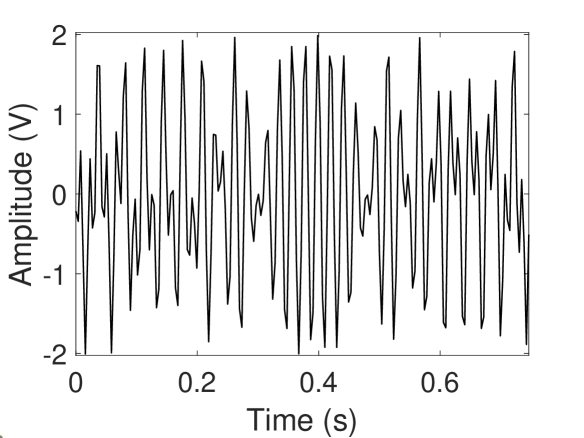
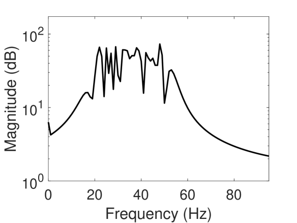
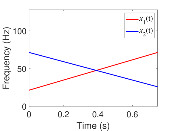
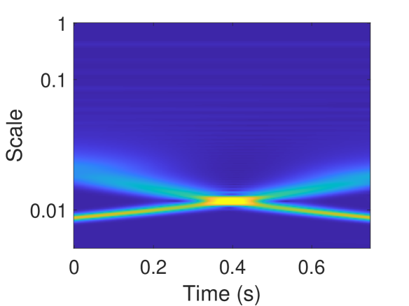
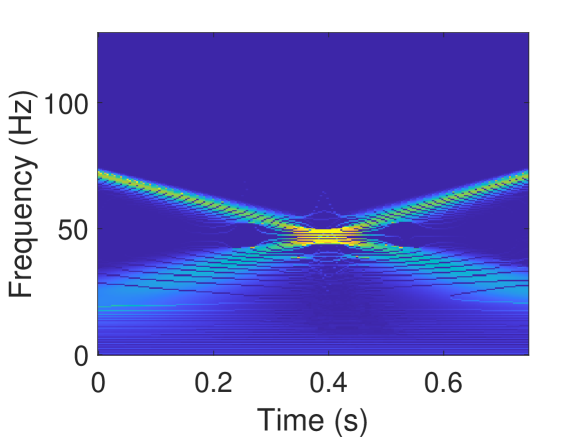
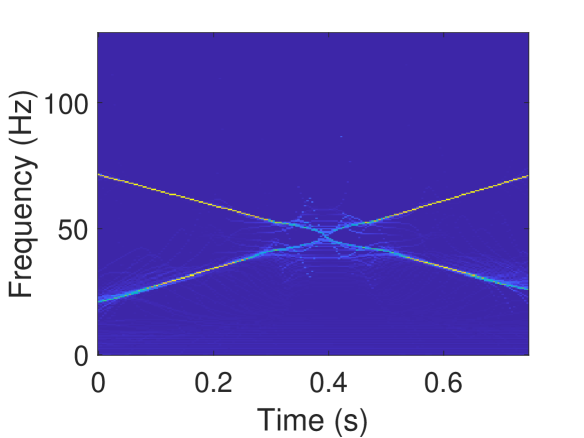
Figure 2: Two-component signal $x(t)$ in (88) and its time-frequency representations with SST. Top row (from left to right): Waveform of $x(t)$, magnitude spectrum and ground truth IFs of two components $x_{1}(t)$ and $x_{2}(t)$; Bottom row (from left to right): CWLT, CWT-based SST and CWT-based second-order SST.

In this section we provide some experimental results to demonstrate our method and general theory. We set $\mu=1$.

Example 1.

Let $x(t)$ be a signal consisting of two-component linear chirps, given as

$$x(t)=x_{1}(t)+x_{2}(t)=\cos(2\pi c_{1}t+\pi r_{1}t^{2})+\cos(2\pi c_{2}t+\pi r_{2}t^{2}),\;t\in[0,0.75),$$ (88)

where $c_{1}=21$, $c_{2}=71$, $r_{1}=67$ and $r_{2}=-61$.

The IFs of $x_{1}$ and $x_{2}$ are $\phi_{1}^{\prime}(t)=c_{1}+r_{1}t$ and $\phi_{2}^{\prime}(t)=c_{2}+r_{2}t$, respectively. See the top-right panel of Figure 2. The chirp rates of $x_{1}$ and $x_{2}$ are $\phi_{1}^{\prime\prime}(t)=r_{1}$ and $\phi_{2}^{\prime\prime}(t)=r_{2}$, respectively. Here signal $x(t)$ is discretized with sampling rate 256Hz. That means there are 192 samples for $x(t)$. In the following, we just use these 192 samples to analyze the signal. The waveform of $x(t)$ and its magnitude spectrum are presented in the top row of Fig.2.

The bottom row of Fig.2 shows the results of CWLT, SST [21] and the second-order SST [37], where parameter $\sigma=0.023$. Here the scale variable $a$ is discretized as $\big{(}2^{j/n_{v}}\triangle t\big{)}_{j}$, where $\triangle t=1/256$ for this example, and $n_{v}$ is the number of voice. Here and below we set $n_{v}=32$. Due to the IF curves of the components are crossover, these methods cannot represent the synthetic signal sharply and separately. In addition, EMD performs poorly in decompose this signal. Consequently, these methods are hardly to recover this two-component signal with crossover IFs.

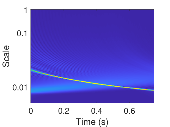
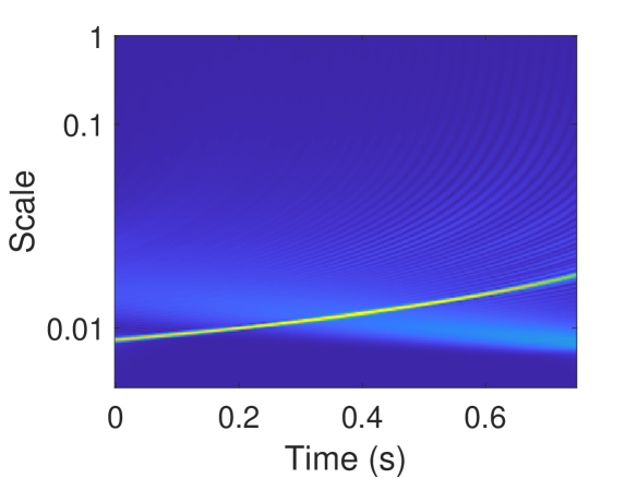
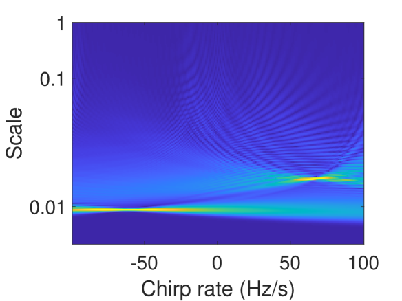
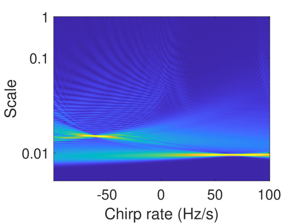
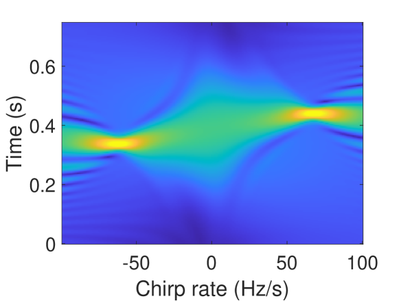
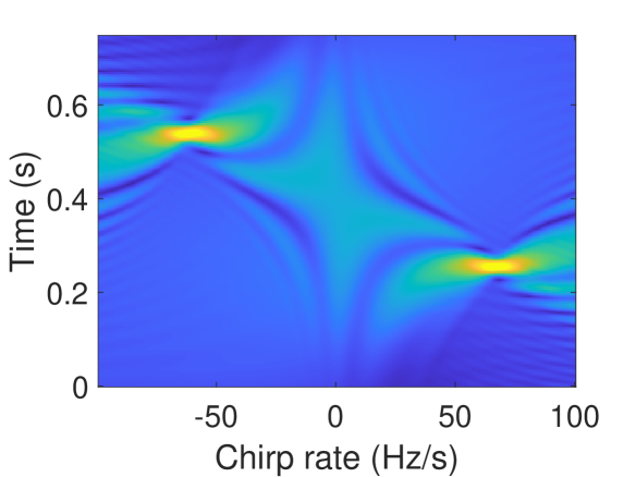
Figure 3: Some slices of adaptive TSC-R. Top row (from left to right): Two slices of $|U_{x}(a,b,\lambda)|$ when $\lambda=r_{1}$, $\lambda=r_{2}$; Middle row (from left to right): Two slices of $|U_{x}(a,b,\lambda)|$ when $b=\frac{32}{256}$ and $b=\frac{160}{256}$; Bottom row (from left to right): Two slices of $|U_{x}(a,b,\lambda)|$ when $a=2^{\frac{51}{32}}/256$ and $a=\frac{1}{64}$.

Next let us look at our method. Due to that the adaptive TSC-R $U_{x}(a,b,\lambda)$ is 3-dimensional, here we show some slices of $|U_{x}(a,b,\lambda)|$. First we look at the slice when $\lambda=r_{1}$, the ground truth chirp rate of $x_{1}$. The top-left panel of Fig.3 is $|U_{x}(a,b,r_{1})|$. The clear and sharp scale-time ridge shown in this panel is exactly the curve $(b,\frac{\mu}{\phi^{\prime}_{1}(b)})$, which gives a precise estimate of $\phi^{\prime}_{1}(b)$, the IF of $x_{1}(t)$. The top-right panel is $|U_{x}(a,b,r_{2})|$, where the clear and sharp scale-time curve corresponds to $(b,\frac{\mu}{\phi^{\prime}_{2}(b)})$. These two pictures tell us that in two scale-time planes (sub-spaces of ${\mathbb{R}}^{3}$) $(b,a,r_{1})$ and $(b,a,r_{2}),b,a\in{\mathbb{R}},a>0$, there do exist two clear and sharp scale-time ridges which are desired to estimate $\phi^{\prime}_{1}(b)$ and $\phi^{\prime}_{2}(b)$. Note that these two scale-time planes are well-separated in the 3-dimensional space ${\mathbb{R}}^{3}$ since the distance between them is $r_{1}-r_{2}=128$, which is large. Thus the estimated chirp rates $\widehat{\lambda}_{1}(b)$ and $\widehat{\lambda}_{2}(b)$ should be easily obtained. In addition, if they are close to $r_{1}$ and $r_{2}$ respectively, then we will have accurate estimates for $\phi^{\prime}_{1}(b)$ and $\phi^{\prime}_{2}(b)$. Here we use the same parameters as those used in Fig.2, especially, $\sigma$ is constant, namely $\sigma=0.023$.

As we see from our theorems that for a given multicomponent signal, the key for the success of our method to recover its modes is: (i) For each $b$, can we obtain $\widehat{a}_{\ell}(b)$ and $\widehat{\lambda}_{\ell}(b)$? and (ii) if yes for Question (i), then whether $\widehat{a}_{\ell}(b)$ and $\widehat{\lambda}_{\ell}(b)$ are close to $\mu/\phi^{\prime}_{\ell}(b)$ and $\phi^{{\prime}{\prime}}_{\ell}(b)$? The answer to Question (ii) is guaranteed by the error bounds in our theorems. So the most important step is whether we can obtain $\widehat{a}_{\ell}(b)$ and $\widehat{\lambda}_{\ell}(b)$. For this example of the two-component signal, the question is for each $b$, two peaks of the function $h(a,\lambda):=|U_{x}(a,b,\lambda)|$ with $a\in(0,\infty),\lambda\in{\mathbb{R}}$ are far apart enough from each other so that we can easily obtain the (local) maximum points $(\widehat{a}_{1},\widehat{\lambda}_{1})$ and $(\widehat{a}_{2},\widehat{\lambda}_{2})$ in the scale-(chirp rate) plane? As examples, in the middle-left panel of Fig.3, we show $h(a,\lambda)$ with $b=32/256$; while $h(a,\lambda)$ with $b=160/256$ is presented in the middle-right panel of Fig.3. From these two panels, we observe that for either $b=32/256$ or $b=160/256$, two peaks of $h(a,\lambda)$ do be far apart and hence we should easily obtain $(\widehat{a}_{1},\widehat{\lambda}_{1})$ and $(\widehat{a}_{2},\widehat{\lambda}_{2})$. Also observe from these two panels, the scale coordinates $\widehat{a}_{1},\widehat{a}_{2}$ of the $(\widehat{a}_{1},\widehat{\lambda}_{1})$ and $(\widehat{a}_{2},\widehat{\lambda}_{2})$ change for different $b=32/256$ or $b=160/256$; while chirp rate coordinates $\widehat{\lambda}_{1},\widehat{\lambda}_{2}$ essentially stay the same (around $70$ and $-60$ respectively). This is due to the fact that $\phi^{\prime}_{1}(b)$ and $\phi^{\prime}_{2}(b)$ change with time $b$, while $\phi^{{\prime}{\prime}}_{1}(b)$ and $\phi^{{\prime}{\prime}}_{2}(b)$ are independent of $b$. In the bottom row of Fig.3, we provide slices $|U_{x}(a,b,\lambda)|$ with $a=2^{\frac{51}{32}}/256$ and $a=1/64$. All these pictures demonstrate that the components $x_{1}$ and $x_{2}$ are well-separated in the 3-dimensional space of adaptive TSC-R, although their IF curves are crossover.

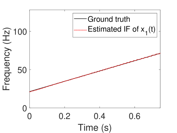
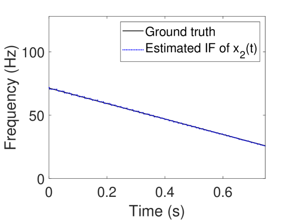
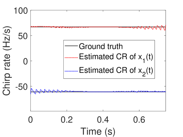
Figure 4: Estimated IF of $x_{1}$ (left panel), estimated IF of $x_{2}$ (middle panel) and estimated chirp rates (right panel) of two components by our method TSC-R.

Fig.4 shows the estimated IFs $\frac{1}{\widehat{a}_{1}(b)},\frac{1}{\widehat{a}_{2}(b)}$ and estimated chirp rates $\widehat{\lambda}_{1}(b)$ and $\widehat{\lambda}_{2}(b)$. Observe the estimated IFs are very close to ground truth $\phi^{{\prime}}_{1}(b)$ and $\phi^{{\prime}}_{2}(b)$. The estimation errors of IFs and chirp rates are mainly caused by the bound effect, which can also be improved with a time-varying $\sigma(b)$. $\blacksquare$

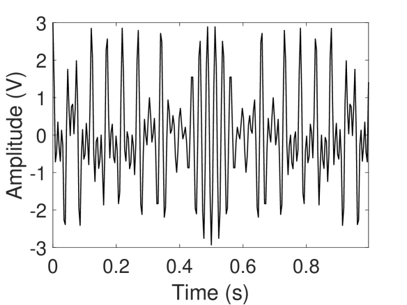
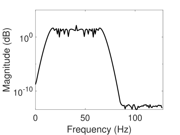
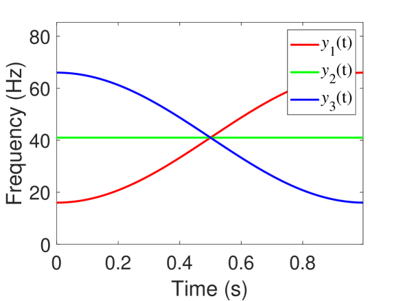
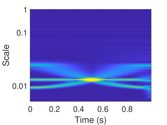
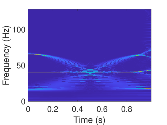
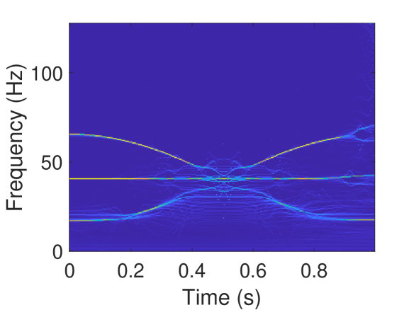
Figure 5: Three-component signal $y(t)$ given in (89) and its time-frequency representations with SST. Top row (from left to right): Waveform of $y(t)$, magnitude spectrum and ground truth IFs of $y_{1}(t)$, $y_{2}(t)$ and $y_{3}(t)$; Bottom row (from left to right): CWLT of $y(t)$, CWT-based SST and CWT-based second-order SST.

Example 2.

Let $y(t)$ be a truncation of the synthetic micro-Doppler signal in Fig.1, given as,

$$y(t)\hskip-17.07182pt =y_{1}(t)+y_{2}(t)+y_{3}(t)$$ (89)

$$=\cos\left(82\pi t+50\cos\big{(}\pi t+\frac{\pi}{2}\big{)}\right)+\cos(82\pi t)+\cos\left(82\pi t+50\cos\big{(}\pi t-\frac{\pi}{2}\big{)}\right),$$

where $t\in[0,1)$.

In the following experiment, $y(t)$ is discretized with the sampling rate 256Hz, namely $t=0,\frac{1}{256},\dots,\frac{255}{256}$. The IFs of $y_{1}$, $y_{2}$ and $y_{3}$ are $\phi_{1}^{\prime}(t)=41-25\sin(\pi t+\frac{\pi}{2})$, $\phi_{2}^{\prime}(t)=41$ and $\phi_{3}^{\prime}(t)=41-25\sin(\pi t-\frac{\pi}{2})$, respectively. See the top-right panel in Fig.5 for IFs. The bottom row of Fig.5 shows CWLT, SST and the second-order SST, where parameter $\sigma=0.023$ and the number of voice $n_{v}=32$. Observed that CWLT and SST are hardly to represent any of these three sub-signals separated and reliably. Thus they cannot separate sub-signals. Actually, as far as we known, there is no efficient algorithm available to recover the three components with the 256 points observation of $y(t)$ above.

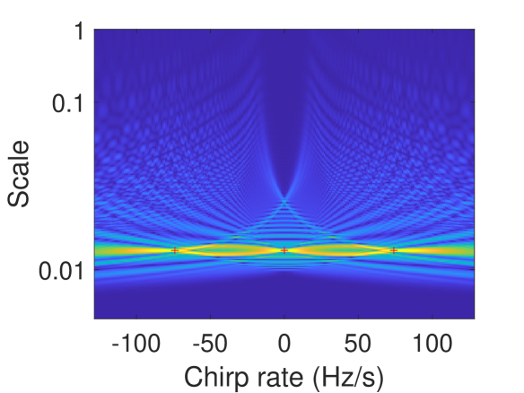
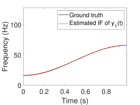
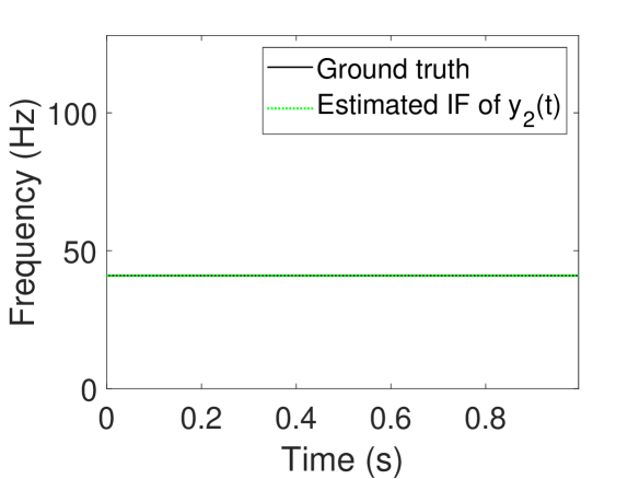
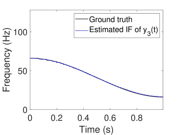
Figure 6: Slice of adaptive TSC-R $|U_{y}(a,b,\lambda)|$ of $y(t)$ when $b=0.5$ (Top-left panel) and estimated IF (dotted lines) of three components (Top-right and bottom panels).

The top-left panel in Fig.6 shows the slice of the adaptive TSC-R $|U_{y}(a,b,\lambda)|$ of $y(b)$ when $b=0.5$, namely the specific time point when the IFs of the three components are crossover. Observe even at this particular time $b=0.5$, the three peaks of $|U_{y}(a,0.5,\lambda)|$ (marked by $+$) are far apart in the scale-(chirp rate) plane. Thus we can easily obtain $(\widehat{a}_{1},\widehat{\lambda}_{1})$, $(\widehat{a}_{2},\widehat{\lambda}_{2})$ and $(\widehat{a}_{3},\widehat{\lambda}_{3})$ for this $b$. Actually for other $b$, three peaks of $|U_{y}(a,b,\lambda)|$ in the scale-(chirp rate) plane are also far apart, and much clearer and sharper than the case here when $b=0.5$. Hence, these three components are well-separated in the 3-dimensional space of $(a,b,\lambda)$. The estimated IF of each component is given in the other panels of Fig.6. The result shows our method is able to estimate the IF of each component correctly and precisely. We provide the result of component recovery in Fig.7, which shows that each recovered waveform is very close to the corresponding mode, except for near time $b=0.5$, where the IFs of three components are crossover. The results show the validity and correctness of the proposed method. Here we use a time-varying parameter $\sigma(b)$, which improves IF estimation and mode recovery performance a lot. How to select $\sigma(b)$ will be addressed in our future work. $\blacksquare$

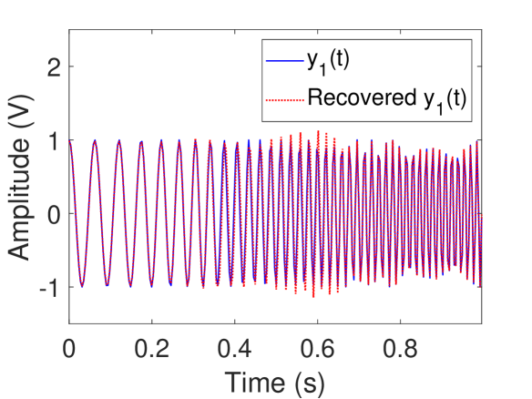
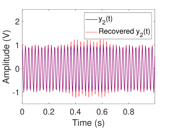
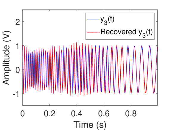
Figure 7: Recovered sub-signals (dotted red lines) of $y_{1}(t)$, $y_{2}(t)$ and $y_{3}(t)$ respectively (from left to right).

Table 1: IF estimate and component recovery errors under white Gaussian noise with different SNRs.

SNR	IF estimate errors			Mode recovery errors
	$\phi_{1}^{\prime}(t)$	$\phi_{2}^{\prime}(t)$	$\phi_{3}^{\prime}(t)$	$y_{1}(t)$	$y_{2}(t)$	$y_{3}(t)$
0 dB	0.1335	0.1361	0.0765	0.7830	0.6457	0.6037
5 dB	0.0281	0.0092	0.0312	0.3183	0.2311	0.3390
10 dB	0.0117	0.0077	0.0162	0.2056	0.1746	0.2506
15 dB	0.0112	0.0005	0.0109	0.1926	0.1241	0.2137
20 dB	0.0099	0.0005	0.0407	0.1927	0.1291	0.2053

Finally, let us consider the effect of our computational scheme for signal data with additive noise, by adding a noise $n(t)$ process to signal $y(t)$ to have a synthetic signal $z(t)$ contaminated by noise $n(t)$:

$$z(t)=y(t)+n(t).$$

Here we let $n(t)$ be a zero-mean Gaussian noise. Table 1 shows the IF estimate and mode recovery errors with different signal-to-noise ratios (SNRs), where the SNR is defined by $10\log_{10}\frac{||y||_{2}}{||n||_{2}}$. The errors in Table 1 are defined by

$$E_{f}=\frac{||f-\widetilde{f}||_{2}}{||f||_{2}},$$

where $\widetilde{f}$ is the estimation of $f$. $E_{f}$ is also called the normalized mean square error. Observe that for SNR$\geq 10$, IF estimation is stable and mode recovery errors are reasonable small.

References

[1] F. Auger, P. Flandrin, Y. Lin, S.McLaughlin, S. Meignen, T. Oberlin, and H.-T. Wu, “Time-frequency reassignment and synchrosqueezing: An overview,” IEEE Signal Process. Mag., vol. 30, no. 6, pp. 32–41, 2013.
[2] R. Behera, S. Meignen, and T. Oberlin, “Theoretical analysis of the 2nd-order synchrosqueezing transform,”
Appl. Comput. Harmon. Anal., vol. 45, no. 2, pp. 379–404, 2018.
[3] A.J. Berrian and N. Saito, “Adaptive synchrosqueezing based on a quilted short-time Fourier transform,”
arXiv:1707.03138v5, Sep. 2017.
[4] H.Y. Cai, Q.T. Jiang, L. Li and B.W. Suter, “Analysis of adaptive short-time Fourier transform-based synchrosqueezing transform,” Analysis and Applications, 2020, in press. arXiv:1812.11033
[5] V.C. Chen, F. Li, S.-S. Ho, and H. Wechsler, “Micro-Doppler effect in radar : phenomenon, model, and simulation study,” IEEE Trans. Aerosp. Electron. Syst., vol. 42, no. 1, pp. 2–21, 2006.
[6] S.S. Chen, D.L. Donoho, and M.A. Saunders, “Atomic decomposition by basis pursuit,” SIAM J. Sci. Comput., vol. 20, no.1, pp. 33–61, 1998.
[7] C.K. Chui and N.N. Han, “Wavelet thresholding for recovery of active sub-signals of a composite signal from its discrete samples,” Appl. Comput. Harmon. Anal., 2020. https://doi.org/10.1016/j.acha.2020.11.003.
[8] C.K. Chui, N.N. Han, and H.N. Mhaskar, “Theory-inspired deep network for instantaneous-frequency extraction and sub-signals recovery from discrete blind-source data,” IEEE Trans. Neural Networks and Learning Systems, submitted for publication, 2020.
[9] C.K. Chui, Q.T. Jiang, L. Li and J. Lu, “Analysis of an adaptive short-time Fourier transform-based multicomponent signal separation method derived from linear chirp local approximation”, preprint, 2020.
[10] C.K. Chui, Q.T. Jiang, L. Lin, and J. Lu, “Adaptive continuous wavelet transform-based signal separation and its analysis,” preprint, 2020.
[11] C.K. Chui, Y.T. Lin, and H.T. Wu, “Real-time dynamics acquisition from irregular samples - with application to anesthesia evaluation,” Anal. Appl., vol. 14, no. 4, pp. 537–590, 2016.
[12] C.K. Chui and H.N. Mhaskar, “Signal decomposition and analysis via extraction of frequencies,” Appl. Comput. Harmon. Anal., vol. 40, no. 1, pp. 97–136, 2016.
[13] C.K. Chui and H.N. Mhaskar, “Naive instantaneous frequency estimation and signal separation from blind source,” in manuscript.
[14] C.K. Chui, H.N. Mhaskar, and M.D. van der Walt, “Data-driven atomic decomposition via frequency extraction of intrinsic mode functions,” Int’l J. Geomath., vol. 7, no.1, pp. 117–146, 2016.
[15] C.K. Chui and M.D. van der Walt, “Signal analysis via instantaneous frequency estimation of signal components,” Int’l J. Geomath., vol. 6, no. 1, pp. 1–42, 2015, 2015.
[16] A. Cicone. “Iterative Filtering as a direct method for the decomposition of nonstationary signals,” Numerical Algorithms, vol. 373, 112248, 2020.
doi: 10.1007/s11075-019-00838-z
[17] A. Cicone, J.F. Liu, and H.M. Zhou, “Adaptive local iterative filtering for signal decomposition and instantaneous frequency analysis,” Appl. Comput. Harmon. Anal., vol. 41, no. 2, pp. 384–411, 2016.
[18] A. Cicone and H.M. Zhou, “Numerical analysis for iterative filtering with new efficient implementations based on FFT,” preprint. Arxiv: 1802.01359.
[19] L. Cohen, Time-frequency Analysis, Prentice Hall, New Jersey, 1995.
[20] R.R. Coifman, “A real variable characterization of of ,” Stud. Math., vol.51, no. 3, pp.269–274, 1974.
[21] I. Daubechies, J.F. Lu, and H.T. Wu, “Synchrosqueezed wavelet transforms: An empirical mode decomposition-like tool,” Appl. Comput. Harmon. Anal., vol. 30, no. 2, pp. 243–261, 2011.
[22] I. Daubechies and S. Maes, “A nonlinear squeezing of the continuous wavelet transform based on auditory nerve models,” in A. Aldroubi, M. Unser Eds. Wavelets in Medicine and Biology, CRC Press, 1996, pp. 527–546.
[23] I. Daubechies, Y. Wang, and H.T. Wu, “ConceFT: Concentration of frequency and time via a multitapered synchrosqueezed transform,” Phil. Trans. Royal Soc. A, vol. 374, no. 2065, Apr. 2016.
[24] P. Flandrin, G. Rilling, and P. Goncalves, “Empirical mode decomposition as a filter bank,” IEEE Signal Proc. Letters, vol. 11, no. 2, pp. 112–114, Feb. 2004.
[25] N.E. Huang, Z. Shen, S.R. Long, M.L. Wu, H.H. Shih, Q. Zheng, N.C. Yen, C.C. Tung, and H.H. Liu, “The empirical mode decomposition and Hilbert spectrum for nonlinear and nonstationary time series analysis,” Proc. Roy. Soc. London A, vol. 454, no. 1971, pp. 903–995, 1998.
[26] Q.T. Jiang and B.W. Suter, “Instantaneous frequency estimation based on synchrosqueezing wavelet transform,” Signal Proc., vol. 138, no. pp. 167–181, 2017.
[27] C. Li and M. Liang, “A generalized synchrosqueezing transform for enhancing signal time-frequency representation,” Signal Proc., vol. 92, no. 9, pp. 2264–2274, 2012.
[28] L. Li, H.Y. Cai, H.X. Han, Q.T. Jiang and H.B. Ji, “Adaptive short-time Fourier transform and synchrosqueezing transform for non-stationary signal separation,” Signal Proc., vol. 166, 2020, 107231.
https://doi.org/10.1016/j.sigpro.2019.07.024
[29] L. Li, H.Y. Cai and Q.T. Jiang, “Adaptive synchrosqueezing transform with a time-varying parameter for non-stationary signal separation,” Appl. Comput. Harmon. Anal., vol. 49, 1075–1106, 2020.
[30] L. Li, H.Y. Cai, Q.T. Jiang and H.B. Ji, “An empirical signal separation algorithm based on linear time-frequency analysis,” Mechanical Systems and Signal Proc.,
vol. 121, pp. 791–809, 2019.
[31] L. Li, C.K. Chui, and Q.T. Jiang, “Direct signals separation via extraction of local frequencies with adaptive time-varying parameters,” preprint, Jan 18, 2020 (submitted to IEEE Trans SP on Jan 21, 2020, ms # T-SP-26004-2020).
[32] L. Li, N.N. Han, Q.T. Jiang, and C.K. Chui, “A separation method for multicomponent non-stationary signals with crossover instantaneous frequencies,” preprint, Feb 8, 2020 (submitted to IEEE Trans IT on Feb 14, 2020, ms # IT-20-0113).
[33] L. Li and H. Ji, “Signal feature extraction based on improved EMD method,” Measurement, vol. 42, pp. 796–803, 2009.
[34] X. Li, G. Bi, S. Stankovic and A.M. Zoubir, “Local polynomial Fourier transform: A review on recent developments and applications,” Signal Proc., vol. 91, no.6, pp.1370–1393, 2011.
[35] L. Lin, Y. Wang, and H.M. Zhou, “Iterative filtering as an alternative algorithm for empirical mode decomposition,” Adv. Adapt. Data Anal., vol. 1, no. 4, pp. 543–560, 2009.
[36] J. Lu, Q.T. Jiang and L. Li, “Analysis of adaptive synchrosqueezing transform with a time-varying parameter,” Advance in Computational Mathematics, vol. 46, Article number: 72, 2020.
https://doi.org/10.1007/s10444-020-09814-x
[37] T. Oberlin and S. Meignen, “The 2nd-order wavelet synchrosqueezing transform,” in 2017 IEEE International Conference on Acoustics, Speech and Signal Processing (ICASSP), March 2017, New Orleans, LA, USA.
[38] T. Oberlin, S. Meignen, and V. Perrier, “The Fourier-based synchrosqueezing transform,” in Proc. 39th Int. Conf. Acoust., Speech, Signal Proc. (ICASSP), 2014, pp. 315–319.
[39] B.G.R. De Prony, “Essai experimental et analytique: sur les lois de la dilatabilite de fluides elastique et sur celles de la force expansive de la vapeur de lalkool, a differentes temperatures,” Journal de lecole polytechnique, vol.1, no. 22, pp. 24 – 76, 1795.
[40] G. Rilling and P. Flandrin, “One or two frequencies? The empirical mode decomposition answers,” IEEE Trans. Signal Proc., vol. 56, pp. 85–95, 2008.
[41] R. Roy and T. Kailath, “ESPRIT-estimation of signal parameters via rotational invariance techniques,” IEEE Trans. Acoustics, Speech, and Signal Proc., vol. 37, no. 7, pp. 984–995, Jul. 1989.
[42] R.O. Schmidt, “Multiple Emitter Location and Signal Parameter Estimation,” IEEE Trans. Antennas and Propagation, vol. 34, no. 3, pp.276–280, Mar. 1986.
[43] Y.L. Sheu, L.Y. Hsu, P.T. Chou, and H.T. Wu, “Entropy-based time-varying window width selection for nonlinear-type time-frequency analysis,” Int’l J. Data Sci. Anal., vol. 3, pp. 231–245, 2017.
[44] L. Stankovi, M. Dakovi, and T. Thayaparan, Time-Frequency Signal Analysis with Applications, Artech House, Boston, 2013.
[45] L. Stankovi, I. Orovi, S. Stankovi, and M. Amin, “Compressive sensing based separation of nonstationary and stationary signals overlapping in time-frequency,” IEEE Trans. Signal Proc., vol 61, no. 18, pp. 4562–4572, Sep. 2013.
[46] G. Thakur and H.T. Wu, “Synchrosqueezing based recovery of instantaneous frequency from nonuniform samples,” SIAM J. Math. Anal., vol. 43, no. 5, pp. 2078–2095, 2011.
[47] M.D. van der Walt, Wavelet Analysis of Non-stationary Signals with Applications, Ph.D. Dissertation, Univ. of Missouri, St. Louis, MO, May 2015.
[48] M.D. van der Walt, “Empirical mode decomposition with shape-preserving spline interpolation,” Results in Applied Mathematics, vol. 5, 100086, Feb. 2020.
[49] S.B. Wang, X.F. Chen, G.G. Cai, B.Q. Chen, X. Li, and Z.J. He, “Matching demodulation transform and synchrosqueezing in time-frequency analysis,” IEEE Trans. Signal Proc., vol. 62, no. 1, pp. 69–84, 2014.
[50] S.B. Wang, X.F. Chen, I.W. Selesnick, Y.J. Guo, C.W. Tong and X.W. Zhang, “Matching synchrosqueezing transform: A useful tool for characterizing signals with fast varying instantaneous frequency and application to machine fault diagnosis,” Mechanical Systems and Signal Proc., vol. 100, pp. 242–288, 2018.
[51] Y. Wang, G.-W. Wei and S.Y. Yang , “Iterative filtering decomposition based on local spectral evolution kernel,” J. Scientific Computing, vol. 50, no. 3, pp. 629–664, 2012.
[52] H.T. Wu, Adaptive Analysis of Complex Data Sets, Ph.D. Dissertation, Princeton Univ., Princeton, NJ, 2012.
[53] Z. Wu and N. E. Huang, “Ensemble empirical mode decomposition: A noise-assisted data analysis method,” Adv. Adapt. Data Anal., vol. 1, no. 1, pp. 1–41, 2009.
[54] Y. Xu, B. Liu, J. Liu, and S. Riemenschneider, “Two-dimensional empirical mode decomposition by finite elements,” Proc. Roy. Soc. London A, vol. 462, no. 2074, pp. 3081–3096, 2006.
[55] H.Z. Yang, “Synchrosqueezed wave packet transforms and diffeomorphism based spectral analysis for 1D general mode decompositions,” Appl. Comput. Harmon. Anal., vol. 39, no.1, pp. 33–66, 2015.
[56] H.Z. Yang and L.X. Ying, “Synchrosqueezed curvelet transform for two-dimensional mode decomposition,” SIAM J. Math Anal., vol 46, no. 3, pp. 2052–2083, 2014.