Convexity and AFPP in the Digital Plane

Abstract

We examine the relationship between convexity and the approximate fixed point property (AFPP) for digital images in ${\mathbb{Z}}^{2}$.

Key words and phrases: digital topology, digital image, convex, approximate fixed point

1 Introduction

The study of fixed points is prominent in many branches of mathematics. In digital topology, it has become worthwhile to broaden the study to “approximate fixed points.” The Approximate Fixed Point Property (AFPP), a generalization of the classical fixed point property (FPP), was introduced in [7]. In this paper, we show that for digital images $X\subset{\mathbb{Z}}^{2}$, convexity can help us show whether $(X,c_{2})$ has the AFPP.

2 Preliminaries

Much of this section is quoted or paraphrased from papers that are listed in the references, especially [4, 5, 6, 7].

We use ${\mathbb{Z}}$ to indicate the set of integers; ${\mathbb{R}}$ for the set of real numbers.

For $(x,y)\in{\mathbb{Z}}^{2}$, the projection functions $pr_{1},pr_{2}:{\mathbb{Z}}^{2}\to{\mathbb{Z}}$ are

$$pr_{1}(x,y)=x,~{}~{}~{}pr_{2}(x,y)=y.$$

2.1 Adjacencies

A digital image is a graph $(X,\kappa)$, where $X$ is a subset of ${\mathbb{Z}}^{n}$ for some positive integer $n$, and $\kappa$ is an adjacency relation for the points of $X$. The $c_{u}$-adjacencies are commonly used. Let $x,y\in{\mathbb{Z}}^{n}$, $x\neq y$, where we consider these points as $n$-tuples of integers:

$$x=(x_{1},\ldots,x_{n}),~{}~{}~{}y=(y_{1},\ldots,y_{n}).$$

Let $u\in{\mathbb{Z}}$, $1\leq u\leq n$. We say $x$ and $y$ are $c_{u}$-adjacent if

• There are at most $u$ indices $i$ for which $|x_{i}-y_{i}|=1$.

• For all indices $j$ such that $|x_{j}-y_{j}|\neq 1$ we have $x_{j}=y_{j}$.

Often, a $c_{u}$-adjacency is denoted by the number of points adjacent to a given point in ${\mathbb{Z}}^{n}$ using this adjacency. E.g.,

• In ${\mathbb{Z}}^{1}$, $c_{1}$-adjacency is 2-adjacency.

• In ${\mathbb{Z}}^{2}$, $c_{1}$-adjacency is 4-adjacency and $c_{2}$-adjacency is 8-adjacency.

• In ${\mathbb{Z}}^{3}$, $c_{1}$-adjacency is 6-adjacency, $c_{2}$-adjacency is 18-adjacency, and $c_{3}$-adjacency is 26-adjacency.

We write $x\leftrightarrow_{\kappa}x^{\prime}$, or $x\leftrightarrow x^{\prime}$ when $\kappa$ is understood, to indicate that $x$ and $x^{\prime}$ are $\kappa$-adjacent. Similarly, we write $x\leftrightarroweq_{\kappa}x^{\prime}$, or $x\leftrightarroweq x^{\prime}$ when $\kappa$ is understood, to indicate that $x$ and $x^{\prime}$ are $\kappa$-adjacent or equal.

A subset $Y$ of a digital image $(X,\kappa)$ is $\kappa$-connected [12], or connected when $\kappa$ is understood, if for every pair of points $a,b\in Y$ there exists a sequence $\{y_{i}\}_{i=0}^{m}\subset Y$ such that $a=y_{0}$, $b=y_{m}$, and $y_{i}\leftrightarrow_{\kappa}y_{i+1}$ for $0\leq i<m$.

Given a digital image $(X,\kappa)$ and $x\in X$, we denote by $N^{*}(X,\kappa,x)$ the set $\{y\in X\,|\,y\leftrightarroweq_{\kappa}x\}$.

2.2 Digitally continuous functions

The following generalizes a definition of [12].

Definition 2.1.

[2] Let $(X,\kappa)$ and $(Y,\lambda)$ be digital images. A single-valued function $f:X\rightarrow Y$ is $(\kappa,\lambda)$-continuous if for every $\kappa$-connected $A\subset X$ we have that $f(A)$ is a $\lambda$-connected subset of $Y$. $\Box$

When the adjacency relations are understood, we will simply say that $f$ is continuous. Continuity can be expressed in terms of adjacency of points:

Theorem 2.2.

[12, 2] A function $f:X\to Y$ is continuous if and only if $x\leftrightarrow x^{\prime}$ in $X$ implies $f(x)\leftrightarroweq f(x^{\prime})$. ∎

See also [8, 9], where similar notions are referred to as immersions, gradually varied operators, and gradually varied mappings.

Let $Y\subset X$ and let $f:X\to Y$ be $(\kappa,\kappa)$-continuous such that $r(y)=y$ for all $y\in Y$. Then $r$ is a $\kappa$-retraction.

The notation $C(X,\kappa)$ denotes $\{f:X\to X\,|\,f\mbox{ is }(\kappa,\kappa)-\mbox{continuous}\}$.

2.3 Approximate fixed points and the AFPP

Let $f\in C(X,\kappa)$ and let $x\in X$. We say

• $x$ is a fixed point of $f$ if $f(x)=x$;

• If $f(x)\leftrightarroweq_{\kappa}x$, then $x$ is an almost fixed point [12, 14] or approximate fixed point [7] of $(f,\kappa)$.

• A digital image $(X,\kappa)$ has the approximate fixed point property (AFPP) [7] if for every $f\in C(X,\kappa)$ there is an approximate fixed point of $f$. This generalizes the fixed point property (FPP): a digital image $(X,\kappa)$ has the FPP if every $f\in C(X,\kappa)$ has a fixed point.

The AFPP gathered attention in part because only a digital image with a single point has the FPP [7].

A. Rosenfeld’s paper [12] states the following as its Theorem 4.1 (quoted verbatim).

Let $I$ be a digital picture, and let $f$ be a continuous function from $I$ into $I$; then there exists a point $P\in I$ such that $f(P)=P$ or is a neighbor or diagonal neighbor of $P$.

We quote from [4]:

Several subsequent papers have incorrectly concluded that this [Rosenfeld’s] result implies that $I$ with some $c_{u}$ adjacency has the $AFPP_{S}$. By digital picture Rosenfeld means a digital cube, $I=[0,n]_{{\mathbb{Z}}}^{v}$. By a “continuous function” he means a $(c_{1},c_{1})$-continuous function; by “a neighbor or diagonal neighbor of $P$” he means a $c_{v}$-adjacent point.

Thus, Rosenfeld’s result was important but weaker than that of Theorem 2.3(6), below.

Theorem 2.3.

The following digital images have the AFPP.

1. Any digital interval $([a,b]_{{\mathbb{Z}}},c_{1})$ [12, 7].

2. Any digital image $(Y,\lambda)$ that is isomorphic to $(X,\kappa)$ such that $(X,\kappa)$ has the AFPP [7]

3. Any digital image $(Y,\kappa)$ that is a retract of $(X,\kappa)$ such that $(X,\kappa)$ has the AFPP [7].

4. Any digital image $(T,\kappa)$ that is a tree [5].

5. Any digital image $(X,c_{m+n})$ such that $X=X^{\prime}\times\Pi_{i=1}^{n}[a_{i},b_{i}]_{{\mathbb{Z}}}$, $X^{\prime}\subset{\mathbb{Z}}^{m}$, and $(X^{\prime},c_{m})$ has the AFPP [5].

6. Any digital cube $(\Pi_{i=1}^{n}[a_{i},b_{i}]_{{\mathbb{Z}}},c_{n})$ [5].

The next result suggests that “most” digital images $(X,c_{u})\subset{\mathbb{Z}}^{v}$ that have the AFPP have $u=v$.

Theorem 2.4.

[4] Let $X\subset{\mathbb{Z}}^{v}$ be such that $X$ has a subset $Y=\Pi_{i=1}^{v}[a_{i},b_{i}]_{{\mathbb{Z}}}$, where $v>1$; for all indices $i$, $b_{i}\in\{a_{i},a_{i}+1\}$; and, for at least 2 indices $i$, $b_{i}=a_{i}+1$. Then $(X,c_{u})$ fails to have the AFPP for $1\leq u<v$.

Example 2.5.

[7] A digital simple closed curve of at least 4 points does not have the AFPP.

2.4 Digital convexity, disks

Material in this section is quoted or paraphrased from [6].

Let $\kappa\in\{c_{1},c_{2}\}$, $n>1$. We say a $\kappa$-connected set $S=\{x_{i}\}_{i=1}^{n}\subset{\mathbb{Z}}^{2}$ is a (digital) line segment if the members of $S$ are collinear.

Remark 2.6.

[6] A digital line segment must be vertical, horizontal, or have slope of $\pm 1$. We say a segment with slope of $\pm 1$ is slanted.

A (digital) $\kappa$-closed curve is a path $S=\{s_{i}\}_{i=0}^{m-1}$ such that $i\neq j$ implies $s_{i}\neq s_{j}$, and $s_{i}\leftrightarrow_{\kappa}s_{(i+1)\mod\,m}$ for $0\leq i\leq m-1$, If $s_{i}\leftrightarrow_{\kappa}s_{j}$ implies $j=(i\pm 1)\mod m$, $S$ is a (digital) $\kappa$-simple closed curve. For a simple closed curve $S\subset{\mathbb{Z}}^{2}$ we generally assume

• $m\geq 8$ if $\kappa=c_{1}$, and

• $m\geq 4$ if $\kappa=c_{2}$.

These requirements are necessary for the Jordan Curve Theorem of digital topology, below, as a $c_{1}$-simple closed curve in ${\mathbb{Z}}^{2}$ needs at least 8 points to have a nonempty finite complementary $c_{2}$-component, and a $c_{2}$-simple closed curve in ${\mathbb{Z}}^{2}$ needs at least 4 points to have a nonempty finite complementary $c_{1}$-component. Examples in [11] show why it is desirable to consider $S$ and ${\mathbb{Z}}^{2}\setminus S$ with different adjacencies.

Theorem 2.7.

[11] (Jordan Curve Theorem for digital topology) Let $\{\kappa,\kappa^{\prime}\}=\{c_{1},c_{2}\}$. Let $S\subset{\mathbb{Z}}^{2}$ be a simple closed $\kappa$-curve such that $S$ has at least 8 points if $\kappa=c_{1}$ and such that $S$ has at least 4 points if $\kappa=c_{2}$. Then ${\mathbb{Z}}^{2}\setminus S$ has exactly 2 $\kappa^{\prime}$-connected components.

One of the $\kappa^{\prime}$-components of ${\mathbb{Z}}^{2}\setminus S$ is finite and the other is infinite. This suggests the following.

Definition 2.8.

[6] Let $S\subset{\mathbb{Z}}^{2}$ be a $c_{2}$-closed curve such that ${\mathbb{Z}}^{2}\setminus S$ has two $c_{1}$-components, one finite and the other infinite. The union $D$ of $S$ and the finite $c_{1}$-component of ${\mathbb{Z}}^{2}\setminus S$ is a (digital) disk. $S$ is a bounding curve of $D$. The finite $c_{1}$-component of ${\mathbb{Z}}^{2}\setminus S$ is the interior of $S$, denoted $Int(S)$, and the infinite $c_{1}$-component of ${\mathbb{Z}}^{2}\setminus S$ is the exterior of $S$, denoted $Ext(S)$.

Note a disk may have multiple distinct bounding curves [6].

More generally, we have the following.

Definition 2.9.

[6] let $X\subset{\mathbb{Z}}^{2}$ be a finite, $c_{i}$-connected set, $i\in\{1,2\}$. Suppose there are pairwise disjoint $c_{2}$-closed curves $S_{j}\subset X$, $1\leq j\leq n$, such that

• $X\subset S_{1}\cup Int(S_{1})$;

• for $j>1$, $D_{j}=S_{j}\cup Int(S_{j})$ is a digital disk;

• no two of

  $$S_{1}\cup Ext(S_{1}),D_{2},\ldots,D_{n}$$

  are $c_{1}$-adjacent or $c_{2}$-adjacent; and

• we have

  $${\mathbb{Z}}^{2}\setminus X=Ext(S_{1})\cup\bigcup_{j=2}^{n}Int(S_{j}).$$

Then $\{S_{j}\}_{j=1}^{n}$ is a set of bounding curves of $X$.

As above, $X$ may have multiple distinct sets of bounding curves.

A set $X$ in a Euclidean space ${\mathbb{R}}^{n}$ is convex if for every pair of distinct points $x,y\in X$, the line segment $\overline{xy}$ from $x$ to $y$ is contained in $X$. The convex hull of $Y\subset{\mathbb{R}}^{n}$, denoted $hull(Y)$, is the smallest convex subset of ${\mathbb{R}}^{n}$ that contains $Y$. If $Y\subset{\mathbb{R}}^{2}$ is a finite set, then $hull(Y)$ is a single point if $Y$ is a singleton; a line segment if $Y$ has at least 2 members and all are collinear; otherwise, $hull(Y)$ is a polygonal disk, and the endpoints of the edges of $hull(Y)$ are its vertices.

A digital version of convexity can be stated for subsets of the digital plane ${\mathbb{Z}}^{2}$ as follows. A finite set $Y\subset{\mathbb{Z}}^{2}$ is (digitally) convex [6] if either

• $Y$ is a single point, or

• $Y$ is a digital line segment, or

• $Y$ is a digital disk with a bounding curve $S$ such that the endpoints of the maximal digital line segments of $S$ are the vertices of $hull(Y)\subset{\mathbb{R}}^{2}$.

3 Retractions, convexity, and the AFPP

Due to assertions (3) and (6) of Theorem 2.3, the following theorem can be useful in determining whether $(X,c_{2})$ has the AFPP, for $X\subset{\mathbb{Z}}^{2}$.

Theorem 3.1.

Let $X\subset Y=[a,b]_{{\mathbb{Z}}}\times[c,d]_{{\mathbb{Z}}}\subset{\mathbb{Z}}^{2}$, such that $X$ is a digitally convex disk. Let $S$ be a bounding curve for $X$. Then there is a $c_{2}$-retraction $r:Y\to X$ such that $r(Y\setminus Int(S))=S$.

Proof.

We define a function $r:Y\to X$ as follows. For $y\in X$, $r(y)=y$.

For $y\not\in X$ we proceed as follows. Let

$$m=\min\{p_{1}(x)\,|\,x\in X\},~{}~{}~{}L=\{x\in S\,|\,p_{1}(x)=m\},$$

$$M=\max\{p_{1}(x)\,|\,x\in X\},~{}~{}~{}R=\{x\in S\,|\,p_{1}(x)=R\}.$$

• Suppose $y=(a,b)$ for $m\leq a\leq M$.

  • If $x=(a,c)\in S$ such that $b>c=\max\{n\,|\,(a,n)\in X\}$ then $r(y)=x$. (See $y_{1},y_{2},y_{3}$ in Figure 1.)

  • If $x=(a,d)\in S$ such that $b<d=\min\{n\,|\,(a,n)\in X\}$ then $r(y)=x$. (See $y_{4}$ in Figure 1.)

• Suppose $y=(a,b)$ for $a<m$; then there is a unique nearest (in the Euclidean metric) $y^{\prime}\in L$ to $y$, determined as follows. Let

  $$s_{0}=\min\{pr_{2}(x)\,|\,x\in L\},~{}~{}~{}s_{1}=\max\{pr_{2}(x)\,|\,x\in L\}.$$

  • If $b>s_{1}$ then $y^{\prime}=(m,s_{1})$. (See $y_{5}$ in Figure 1.)

  • If $s_{0}\leq b\leq s_{1}$ then $y^{\prime}=(m,b)$. (See $y_{6}$ in Figure 1.)

  • If $b<s_{0}$ then $y^{\prime}=(m,s_{0})$. (See $y_{7}$ in Figure 1.)

  Let $r(y)=y^{\prime}$.

• Suppose $y=(a,b)$ for $a>M$; then there is a unique nearest (in the Euclidean metric) $y^{\prime}\in L$ to $y$, determined as follows. Let

  $$s_{2}=\min\{pr_{2}(x)\,|\,x\in R\},~{}~{}~{}s_{3}=\max\{pr_{2}(x)\,|\,x\in R\}.$$

  • If $b>s_{3}$ then $y^{\prime}=(M,s_{3})$. (See $y_{8}$ in Figure 1.)

  • If $s_{2}\leq b\leq s_{3}$ then $y^{\prime}=(M,b)$. (See $y_{9}$ in Figure 1.)

  • If $b<s_{2}$ then $y^{\prime}=(M,s_{2})$. (See $y_{10}$ in Figure 1.)

  Let $r(y)=y^{\prime}$.

In order to show $r$ is a $c_{2}$-retraction, we must show $r\in C(X,c_{2})$. Let $y\leftrightarrow_{c_{2}}y^{\prime}$ in $X$.

• Suppose $y\in X$.

  • If $y^{\prime}\in X$, then we have $r(y^{\prime})=y^{\prime}\leftrightarrow_{c_{2}}y=r(y)$.

  • If $y^{\prime}\not\in X$ then we must have $y\in S$. Then either $r(y^{\prime})=r(y)$, or, since $X$ is convex, it follows from Remark 2.6 that $r(y^{\prime})\leftrightarrow_{c_{2}}y=r(y)$.

• Suppose $y$ is vertically above or below a point $x\in S$, so $r(y)=x$. Since $X$ is convex, it follows from Remark 2.6 that $r(y^{\prime})\leftrightarroweq_{c_{2}}x=r(y)$.

• Suppose $p_{1}(y)<m$. Since $X$ is convex, it follows from Remark 2.6 that $r(y^{\prime})\leftrightarroweq_{c_{2}}r(y)$.

• Suppose $p_{1}(y)>M$. Since $X$ is convex, it follows from Remark 2.6 that $r(y^{\prime})\leftrightarroweq_{c_{2}}r(y)$.

Thus $r\in C(X,c_{2})$. Therefore, $r$ is a retraction. Clearly, $r(Y\setminus Int(S))=S$. This completes the proof. ∎

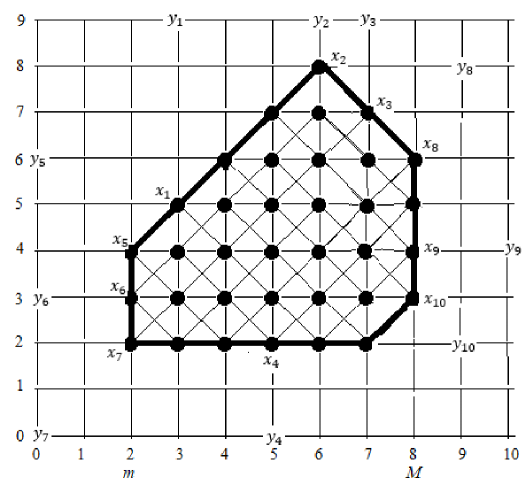
Figure 1: Retraction $r$ of a digital image $Y$ to a subset $X$ that is a convex disk as in Theorem 3.1. Here, $s_{0}=2$, $s_{1}=4$, $s_{2}=3$, $s_{3}=6$.
a) Each point vertically above or below the disk is mapped to its nearest vertical neighbor in $X$, e.g., $r(y_{i})=x_{i}$, $i\in\{1,2,3,4\}$.
b) Each point to the left (not necessarily horizontally) of $X$ is mapped to the nearest member of $X$ with minimal first coordinate, e.g., $r(y_{i})=x_{i}$, $i\in\{5,6,7\}$.
c) Each point to the right (not necessarily horizontally) of $X$ is mapped to the nearest member of $X$ with maximal first coordinate, e.g., $r(y_{i})=x_{i}$, $i\in\{8,9,10\}$.

Theorem 3.2.

Let $X\subset Y=[a,b]_{{\mathbb{Z}}}\times[c,d]_{{\mathbb{Z}}}\subset{\mathbb{Z}}^{2}$, such that $X$ is digitally convex. Then $(X,c_{2})$ has the AFPP.

Proof.

By Theorem 2.3(5), $(Y,c_{2})$ has the AFPP. By Theorem 3.1, $(X,c_{2})$ is a retract of $(Y,c_{2})$. By Theorem 2.3(3), $(X,c_{2})$ has the AFPP. ∎

Corollary 3.3.

Let $X=X_{1}\times X_{2}$, where $X_{1}\subset{\mathbb{Z}}^{n}$, $(X_{1},c_{n})$ has the AFPP, $X_{2}\subset{\mathbb{Z}}^{2}$, and $X_{2}$ is a digitally convex disk. Then $(X,c_{n+2})$ has the AFPP.

Proof.

Clearly there exists $Y=[a,b]_{{\mathbb{Z}}}\times[c,d]_{{\mathbb{Z}}}$ such that $X_{2}\subset Y$. By Theorem 2.3(4), $(X_{1}\times Y,c_{n+2})$ has the AFPP. By Theorem 3.1, there is a $c_{2}$-retraction $r:Y\to X_{2}$. Then $\operatorname{id}_{X_{1}}\times r:X_{1}\times Y\to X$ is a $c_{n+2}$-retraction. The assertion follows from Theorem 2.3(3). ∎

Proposition 3.4.

Let $X\subset{\mathbb{Z}}^{2}$ be finite. Suppose $X^{\prime}\subset{\mathbb{Z}}^{2}$ is a convex disk with bounding curve $S$ such that $X^{\prime}\setminus Int(S)$ is a $c_{2}$-component of ${\mathbb{Z}}^{2}\setminus X$. Then there is a $c_{2}$-retraction of $X$ onto $S$.

Proof.

By Theorem 3.1, there is a $c_{2}$-retraction $r:X\cup X^{\prime}\to X^{\prime}$ such that $r(X)=S$. Then $r|_{X}:X\to S$ is a retraction. ∎

Theorem 3.5.

Let $X\subset{\mathbb{Z}}^{2}$ be finite. Suppose $X^{\prime}\subset X$ is a convex disk with bounding curve $S$ such that $X^{\prime}\setminus S$ is a $c_{2}$-component of ${\mathbb{Z}}^{2}\setminus X$. Suppose there is a continuous $F:S\to S$ such that

$$\mbox{for each }x\in S,~{}N^{*}(X,\kappa,x)\cap N^{*}(X,\kappa,F(x))=\emptyset.$$ (1)

Then $(X,c_{2})$ does not have the AFPP.

Proof.

By Proposition 3.4, there is a $c_{2}$-retraction $r:X\to S$. Let $F$ be as described above and let $f:X\to X$ be the function $f(x)=F\circ r(x)$. Since composition preserves continuity, we have $f\in C(X,c_{2})$.

Consider the following cases.

• Suppose $y\not\leftrightarroweq_{c_{2}}x$ for all $x\in S$. Then in particular, $y\not\leftrightarroweq_{c_{2}}f(y)$, so $y$ is not an approximate fixed point for $f$.

• Suppose $y\leftrightarroweq_{c_{2}}x$ for some $x\in S$. Then the continuity of $f$ implies $f(y)\leftrightarroweq_{c_{2}}f(x)$. It follows from (1) that $y$ is not an approximate fixed point for $f$.

Thus $f$ does not have an approximate fixed point. The assertion follows. ∎

Example 3.6.

Let $X=[-3,3]_{{\mathbb{Z}}}^{2}\setminus A$, where $A=\{(x,y)\in{\mathbb{Z}}^{2}~{}|~{}|x|+|y|\leq 1\}$. See Figure 2. As a bounding curve for $A$, we can take $S=\{(x,y)\in{\mathbb{Z}}^{2}~{}|~{}|x|+|y|=2\}$. Then $S$ is a $c_{2}$-simple closed curve. Let $F:S\to S$ be the map $F(x,y)=(-x,-y)$. Then we may apply Theorem 3.5 to conclude that $(X,c_{2})$ does not have the AFPP.

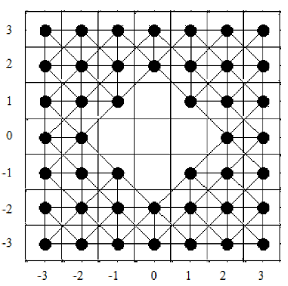
Figure 2: The image $X$ of Example 3.6

4 Further remarks

We have explored relationships between the convexity of digital images in ${\mathbb{Z}}^{2}$ and the AFPP.

In classical topology, every absolute retract (a contractible compactum with certain “nice” local properties for which we need not consider analogs in digital topology) has the FPP [1]. Since under the definition of digital homotopy in [2], a digital simple closed curve of 4 points is digitally contractible [3], Example 2.5 shows that contractibility based on [2] is not sufficient for the AFPP. Recent papers of Staecker [13] and Lupton, Oprea, and Scoville [10] have developed a different notion of homotopy under which a digital simple closed curve of 4 points is not digitally contractible; Staecker calls this strong homotopy. This suggests the following questions concerning possible extensions of Theorem 3.2.

Question 4.1.

Let $X\subset{\mathbb{Z}}^{2}$ be finite and $c_{2}$-strongly contractible, i.e., contractible with respect to strong homotopy. Does $(X,c_{2})$ have the AFPP?

If Question 4.1 and the following Question 4.2 both have affirmative answers, the latter result would be contained in the former.

Question 4.2.

Let $X\subset{\mathbb{Z}}^{2}$ be a digital disk. Does $(X,c_{2})$ have the AFPP?

References

[1]
K. Borsuk,
Theory of Retracts,
Polish Scientific Publishers, Warsaw, 1967.
[2]
L. Boxer,
A classical construction for the digital fundamental group,
Pattern Recognition Letters 10 (1999), 51-62.
[3]
L. Boxer, Properties of digital homotopy,
Journal of Mathematical Imaging and Vision 22 (2005), 19-26.
[4]
L. Boxer, Approximate Fixed Point Properties in Digital Topology,
Bulletin of the International Mathematical Virtual Institute 10 (2) (2020), 357-367.
[5]
L. Boxer, Approximate Fixed Point Property for Digital Trees and Products,
Bulletin of the International Mathematical Virtual Institute 10 (3) (2020), 595-602.
[6]
L. Boxer,
Convexity and freezing sets in digital topology,
Applied General Topology, to appear.
Available at https://arxiv.org/abs/2005.09713
[7]
L. Boxer, O. Ege, I. Karaca, J. Lopez, and J. Louwsma, Digital Fixed Points,
Approximate Fixed Points, and Universal Functions,
Applied General Topology 17(2), 2016, 159-172.
[8]
L. Chen, Gradually varied surfaces and its optimal uniform approximation,
SPIE Proceedings 2182 (1994), 300-307.
[9]
L. Chen, Discrete Surfaces and Manifolds, Scientific Practical Computing,
Rockville, MD, 2004
[10]
G. Lupton, J. Oprea, and N. Scoville,
Homotopy theory in digital topology, preprint.
Available at https://arxiv.org/abs/1905.07783
[11]