Time-Transformed Test for Bubbles under Non-stationary Volatility

Abstract

This paper is devoted to testing for bubbles under time-varying non-stationary volatility. Because the limiting distribution of the seminal Phillips et al., (2011) test depends on the variance function and usually requires a bootstrap implementation under heteroskedasticity, we construct the test based on a deformation of the time domain. The proposed test is asymptotically pivotal under the null hypothesis and its limiting distribution coincides with that of the standard test under homoskedasticity, so that the test does not require computationally extensive methods for inference. Appealing finite sample properties are demonstrated through Monte-Carlo simulations. An empirical application demonstrates that the upsurge behaviour of cryptocurrency time series in the middle of the sample is partially explained by the volatility change.

Keywords: Rational bubble; Explosive autoregression; Time-varying volatility; Right-tailed unit root testing; Variance profile; Time-transformed data

JEL Codes: C12, C22

1 Introduction

In this paper, we consider testing for bubbles under heteroskedastic volatility. Since a seminal paper of Phillips et al., (2011) testing for and dating for rational bubbles have been investigated in both the theoretical and empirical econometrics literature. Because time series characterized by an explosive behaviour may be modeled by a process with an autoregressive time-varying coefficient, Phillips et al., (2011) and Phillips et al., 2015a , Phillips et al., 2015b proposed constructing subsample ADF-type statistics that take the supremum over the subsamples. Homme and Breitung, (2012) compared the subsample ADF-type test with several other alternative tests, including the Chow-type unit root statistics, while Whitehouse, (2019) considered the Phillips et al., (2011) test with the GLS-type detrending. Note that these studies assumed that volatility in the shocks is constant over the sample period. However, it is well known in the empirical finance literature that volatility in financial time series may not be constant but change depending on time. In this case, the above tests for bubbles may suffer from size distortion because the limiting distributions of the test statistics depend on the volatility structure, as demonstrated by Cavaliere, (2004), Cavaliere and Taylor, 2007a , Cavaliere and Taylor, 2007b , Cavaliere and Taylor, (2008), inter alia, in the unit root testing literature and by Harvey et al., (2016) for the Phillips et al., (2011) test.

To address this issue, several papers proposed testing for the explosive behaviour under time-varying volatility. Harvey et al., (2016) showed that the limiting distribution of the supremum ADF (SADF) test of Phillips et al., (2011) depends on the so-called variance profile, which will be defined in Section 3, and proposed a wild bootstrap implementation to obtain the asymptotically correct size of the test. Hafner, (2020) modified the wild bootstrap algorithm of Harvey et al., (2016) to allow the skewed distribution of the series. Harvey et al., (2019) proposed a weighted least squares based modification of the SADF test with a non-parametric kernel smoothing estimator of the variance process (their test is called SBZ test). The limit distribution of the test still depends on the variance profile under the null and local alternatives and the test also has a non-monotonic power problem in some cases. Harvey et al., (2019) suggested to use a union of rejections testing strategy based on two tests, the SBZ and the SADF (under this strategy, we reject the null of a unit root if at least one of the tests in a union rejects the null), coupling with a wild bootstrap implementation of Harvey et al., (2016). Harvey et al., (2020) proposed another method which controls size under time-varying volatility. This method is based on the cumulated signs of the first differences of the dependent variable and leads to the pivotal null limiting distribution under time-varying volatility. However, under the local alternative, the sign-based test depends on volatility function, and Harvey et al., (2020) suggested to use a wild bootstrap based union of rejections testing strategy with the SADF and sign-based tests. However, these tests are computationally expensive, and computation time increases rapidly if the sample size increases. Finally, Astill et al., (2021) developed a CUSUM-based monitoring procedure for explosive episodes which is robust to time-varying volatility.

In this paper, we propose a new method for testing the explosive behaviour under nonstationary volatility ($\sigma_{t}$) by transforming the series according to the volatility behaviour, similarly to Cavaliere and Taylor, 2007b in the unit root testing context. More precisely, we take the sampling interval longer in the low volatility regime, whereas we take it shorter for large values of $\sigma_{t}$. We construct the test statistic based on transformed data that has the same limiting distribution as its standard counterpart constructed under homoskedasticity. The transformation of the time series is based on the variance profile estimated from data. For this, we utilise the approach of Harvey et al., (2021); we estimate non-parametrically the time-varying autoregressive coefficient, collect residuals, and use them for estimating the variance profile. The supremum based test for the bubbles is constructed in a simple way based on the transformed version of the subsample tests. Monte-Carlo simulations demonstrate that our test proposed in this paper can control the empirical size well and is most powerful among the other existing tests in some cases, although the latter is not always the case and our test is less powerful in other cases. Thus, the contribution of this paper is the proposal of new tests with well controlled size. As a by-product of using the asymptotic critical values, our method is computationally less expensive comparing to the existing methods with the bootstrap method. An empirical application demonstrates that it is important to take non-stationary volatility into account when testing for a bubble in the time-series possibly with unstable volatility.

The paper is organized as follows. Section 2 formulates the model and assumptions. In Section 3 we propose to implement a deformation of the time domain for the time series and use the transformed series to construct the SADF type test statistic for the explosive behaviour. Using this time deformation with the variance profile assumed to be known, we show that the limiting distribution of the test statistic is the same as in the case of homoskedasticity. Section 4 discusses the case of the unknown variance profile and the corresponding limiting result. Monte-Carlo simulations are performed in Section 5. Section 6 gives the empirical application, and Section 7 concludes the paper.

2 Model and Assumptions

Consider the time series $\{y_{t}\}$ generated by the following data generating process (DGP) that allows one explosive regime with a subsequent collapsing regime:

$$y_{t} = \mu+u_{t},$$ (1)

$$u_{t} = \begin{cases}u_{t-1}+\varepsilon_{t},&t=1,\dots,\lfloor\tau_{1,0}T\rfloor,\\ (1+\delta_{1})u_{t-1}+\varepsilon_{t},&t=\lfloor\tau_{1,0}T\rfloor+1,\dots,\lfloor\tau_{2,0}T\rfloor,\\ (1-\delta_{2})u_{t-1}+\varepsilon_{t},&t=\lfloor\tau_{2,0}T\rfloor+1,\dots,\lfloor\tau_{3,0}T\rfloor,\\ u_{t-1}+\varepsilon_{t},&t=\lfloor\tau_{3,0}T\rfloor+1,\dots,T,\\ \end{cases}$$ (2)

$$\varepsilon_{t} = \sigma_{t}e_{t}$$ (3)

where $\delta_{1}\geq 0$, $\delta_{2}\geq 0$, $0\leq\tau_{1,0}<\tau_{2,0}\leq\tau_{3,0}\leq 1$, and the initial value condition is given by $u_{0}=o_{p}(\sqrt{T})$. We assume that $\mu=0$ for simplicity but a positive shrinking drift may be allowed as considered by Phillips et al., (2014) and Phillips et al., 2015a , Phillips et al., 2015b . The process $\{y_{t}\}$ evolves as a unit root process, but a bubble possibly emerges at $\lfloor\tau_{1,0}T\rfloor+1$ ($\lfloor\cdot\rfloor$ denotes an integer part of value) with the explosive AR(1) coefficient given by $1+\delta_{1}$, followed by the collapsing regime from $\lfloor\tau_{2,0}T\rfloor+1$ to $\lfloor\tau_{3,0}T\rfloor$ generated as a stationary process, which is interpreted as the return to the normal market behaviour. The magnitude of $\delta_{2}$ specifies the extent of the collapse of the bubble with the duration between $\lfloor\tau_{2,0}T\rfloor+1$ and $\lfloor\tau_{3,0}T\rfloor$. When a crash occurs, we assume, following Harvey et al., (2021), that $y_{\lfloor\tau_{3,0}T\rfloor}\coloneqq y^{*}a_{T}$, where $y^{*}=O_{p}(1)$ and $a_{T}=1$ or $a_{T}\to\infty$. The volatility of the innovations is given by $\sigma_{t}$ and it can be non-stationary. Note that we can simply rewrite the process for $\{y_{t}\}$ as

$$y_{t}=(1+\delta_{t})y_{t-1}+\varepsilon_{t}\qquad\mbox{or}\qquad\Delta y_{t}=\delta_{t}y_{t-1}+\varepsilon_{t}$$ (4)

with obvious definition of $\delta_{t}$. The null hypothesis we consider is that the market is efficient and thus $\delta_{t}=0$ in expression (4). On the other hand, we assume the existence of a bubble under the alternative, which corresponds to the case where $\delta_{t}$ in (4) is not stable at 1 and the model is given by (1)–(3) with $\delta_{1}>0$.

We suppose that the following assumption holds.

Assumption 1

(a) $\{e_{t}\}$ is a martingale difference sequence with respect to $\mathcal{F}_{t}\coloneqq\sigma(e_{t},e_{t-1},\ldots)$ with $E[e_{t}^{2}|\mathcal{F}_{t-1}]=1$ and $E[|e_{t}|^{p}|\mathcal{F}_{t-1}]<\infty$ almost surely for some $p>6$. (b) The volatility $\sigma_{t}$ is defined as $\sigma_{t}\coloneqq\omega(t/T)$, where $\omega(s)\in D[0,1]$ for $s\in[0,1]$ is a non-stochastic and strictly positive function satisfying $0<\underline{\omega}<\omega(s)<\bar{\omega}<\infty$.

Assumption 1(a) requires the existence of more than 6-th order moments, which is used for the nonparametric estimation of the AR(1) coefficient. Assumption 1(b) allows a general class of volatility processes; we can allow breaks in volatility, trending volatility, and regime switching volatility. See, for example, Cavaliere and Taylor, 2007a , Cavaliere and Taylor, 2007b . Note that under homoskedasticity, $\sigma_{t}$ reduces to $\sigma$ for all $t$. Under Assumption 1, the conditional variance of $\varepsilon_{t}$ is given by $E[\varepsilon_{t}|{\cal F}_{t-1}]=\sigma_{t}^{2}$ and thus conditional heteroskedasticity is allowed in the model. Although the conditional and unconditional variances are the same ($\sigma_{t}^{2}$) under Assumption 1, our model can flexibly capture the typical property of financial data such as volatility clustering because $\sigma_{t}$ covers a wide class of nonlinear functions.

Under Assumption 1, the partial sum process of $\{\varepsilon_{t}\}$ is asymptotically characterized by the variance profile, termed by Cavaliere and Taylor, 2007a , which is defined as

$$\eta(s)\coloneqq\left(\int_{0}^{1}\omega(r)^{2}dr\right)^{-1}\int_{0}^{s}\omega(r)^{2}dr.$$

We also define the so called (asymptotic) average innovation variance as

$$\bar{\omega}^{2}\coloneqq\int_{0}^{1}\omega(r)^{2}dr.$$

Note that $\eta(s)=s$ under homoskedasticity. Then, under Assumption 1, we have the following weak convergence due to Theorem 1 of Cavaliere and Taylor, 2007a :

$$\frac{1}{\sqrt{T}}y_{\lfloor rT\rfloor}=\frac{1}{\sqrt{T}}u_{\lfloor rT\rfloor}=\frac{1}{\sqrt{T}}\sum_{t=1}^{\lfloor rT\rfloor}\varepsilon_{t}\Rightarrow\bar{\omega}W(\eta(r))\eqqcolon\bar{\omega}W^{\eta}(r)\qquad(0\leq r\leq 1),$$ (5)

where $\Rightarrow$ denote weak convergence in $D[0,1]$ and $W(\cdot)$ is a standard Brownian motion, while $W^{\eta}(\cdot)$ is called a variance transformed Brownian motion (Brownian motion under a modification of the time domain). Again, we can see that in the case of a constant variance with $\sigma_{t}=\sigma$, we have $\eta(r)=r$ and thus $W^{\eta}(r)$ reduces to a standard Brownian motion.

3 Deformation of Time Domain When the Variance Profile is Known

In this section, we propose new tests for a bubble under the infeasible assumption that the variance profile is known. We will show that the new test statistics are asymptotically pivotal and thus can be implemented with the asymptotic critical values. The feasible versions will be considered in the next section.

To propose new test statistics, we first review the methodology proposed by Phillips et al., (2011), which utilize the maximum of the ADF test statistics constructed using subsamples. Let $ADF_{r_{1}}^{r_{2}}$ be the ADF $t$-statistic of $\delta$ in the regression

$$\Delta y_{t}=\mu+\delta y_{t-1}+\varepsilon_{t}$$ (6)

for $t=\lfloor r_{1}T\rfloor+1$ to $\lfloor r_{2}T\rfloor$. Then, the so-called SADF test statistic is defined as

$$SADF\coloneqq\sup_{r_{2}\in[r_{0},1]}ADF_{0}^{r_{2}}$$ (7)

where the right-tail is the rejection region. Furthermore, the SADF test is extended to multiple bubble context in Phillips et al., 2015a , Phillips et al., 2015b and the generalized SADF (GSADF) test statistic is given by

$$GSADF(r_{0})\coloneqq\sup_{r_{2}\in[r_{0},1],r_{1}\in[0,r_{2}-r_{0}]}ADF_{r_{1}}^{r_{2}}.$$ (8)

In this form, $r_{\omega}\coloneqq r_{2}-r_{1}$ is a window size with the minimum size as $r_{0}$. That is, for every given $r_{2}$, the ADF test statistic is calculated over all possible $r_{1}$ from 0 to $r_{2}-r_{0}$ and the GSADF test is constructed as the maximum of them. Note that the SADF test is the special case of the GSADF test by setting $r_{1}=0$ and $r_{2}=r_{\omega}\in[r_{0},1]$.

These two tests are based on regression (6) and we typically include a constant even if we assume $\mu=0$, because the effect of the initial value disappears under the null hypothesis by including a constant. We call this method the OLS-demeaning. On the other hand, Whitehouse, (2019) proposed the GLS-type demeaning, which results in the increase of power in some cases.

Although the SADF and GSADF test statistics are asymptotically pivotal under the assumption of homoskedasticity, it is not difficult to see, as demonstrated by Harvey et al., (2016) and Harvey et al., (2019), that their limiting distributions depend on the volatility process through the variance profile $\eta(s)$ under the existence of heteroskedasticity. In the following, we briefly investigate this dependence to explain our motivation for the construction of new test statistics.

Following Harvey et al., (2019), we consider the SADF test statistic with a version of the GLS-type demeaning; we subtract the initial value of $y$ from all the observations, which is given by $\check{y}_{t}\coloneqq y_{t}-y_{0}$. We call this specific treatment the GLS-demeaning. In this case, the test statistic is constructed from (6) without a constant and thus $ADF_{r_{1}}^{r_{2}}$can be written as

$$ADF_{r_{1}}^{r_{2}}\coloneqq\frac{\sum_{t=\lfloor r_{1}T\rfloor+1}^{\lfloor r_{2}T\rfloor}\check{y}_{t-1}\Delta\check{y}_{t}}{\sqrt{\hat{\sigma}^{2}(r_{1},r_{2})\sum_{t=\lfloor r_{1}T\rfloor+1}^{\lfloor r_{2}T\rfloor}\check{y}_{t-1}^{2}}},$$ (9)

where $\hat{\sigma}^{2}(r_{1},r_{2})$ is the usual variance estimator based on the regression residuals in this subsample. From (5), we can deduce that under the null hypothesis,

$$\frac{1}{T}\sum_{t=\lfloor r_{1}T\rfloor+1}^{\lfloor r_{2}T\rfloor}\check{y}_{t-1}\Delta\check{y}_{t} = \frac{1}{2T}\left[\check{y}_{\lfloor r_{2}T\rfloor}^{2}-\check{y}_{\lfloor r_{1}T\rfloor}^{2}-\sum_{t=\lfloor r_{1}T\rfloor+1}^{\lfloor r_{2}T\rfloor}(\check{y}_{t}-\check{y}_{t-1})^{2}\right]$$ (10)

$$\Rightarrow \frac{1}{2}\left(\bar{\omega}^{2}W^{\eta}(r_{2})^{2}-\bar{\omega}^{2}W^{\eta}(r_{1})^{2}-\int_{r_{1}}^{r_{2}}\omega(r)^{2}dr\right),$$ (11)

$$\frac{1}{T^{2}}\sum_{t=\lfloor r_{1}T\rfloor+1}^{\lfloor r_{2}T\rfloor}\check{y}_{t-1}^{2} \Rightarrow \bar{\omega}^{2}\int_{r_{1}}^{r_{2}}(W^{\eta}(r))^{2}dr,$$ (12)

$$\hat{\sigma}^{2}(r_{1},r_{2}) \rightarrow_{p} \frac{1}{r_{2}-r_{1}}\int_{r_{1}}^{r_{2}}\omega(r)^{2}dr.$$ (13)

As a result, we obtain the following proposition, which is also stated in Harvey et al., (2019).

Proposition 1

Suppose that Assumption 1 holds. Under the null hypothesis, we have, with the GLS-demeaning,

$$SADF\Rightarrow\sup_{r_{2}\in[r_{0},1]}\widetilde{ADF}_{0}^{r_{2}}(\omega)\quad\mbox{and}\quad GSADF(r_{0})\Rightarrow\sup_{r_{2}\in[r_{0},1],r_{1}\in[0,r_{2}-r_{0}]}\widetilde{ADF}_{r_{1}}^{r_{2}}(\omega),$$

$$\mbox{where}\quad\widetilde{ADF}_{r_{1}}^{r_{2}}(\omega)\coloneqq\frac{\bar{\omega}\left(W^{\eta}(r_{2})^{2}-W^{\eta}(r_{1})^{2}-\cfrac{\int_{r_{1}}^{r_{2}}\omega(r)^{2}dr}{\bar{\omega}^{2}}\right)}{2\sqrt{\frac{1}{r_{2}-r_{1}}\int_{r_{1}}^{r_{2}}\omega(r)^{2}dr}\sqrt{\int_{r_{1}}^{r_{2}}(W^{\eta}(r))^{2}dr}}.$$ (14)

We can see that the limiting distribution of the $ADF_{r_{1}}^{r_{2}}$ statistic depends on a variance-transformed Brownian motion, which in turn depends on the variance profile. Similarly, $ADF_{r_{1}}^{r_{2}}$ with the OLS-demeaning also depends on the variance structure as shown by Harvey et al., (2016). As a result, we cannot control the size of the test by using the critical values obtained under the assumption of homoskedasticity. Note that, in the special case of homoskedasticity with $\sigma_{t}=\sigma$, $\widetilde{ADF}_{r_{1}}^{r_{2}}$ reduces to the well-known form given by

$$\widetilde{ADF}_{r_{1}}^{r_{2}}(1)\coloneqq\frac{W(r_{2})^{2}-W(r_{1})^{2}-(r_{2}-r_{1})}{2\sqrt{\int_{r_{1}}^{r_{2}}W(r)^{2}dr}},$$ (15)

and thus, the distribution becomes free of the variance profile in this case.

To overcome this problem, Harvey et al., (2016) and Harvey et al., (2019) proposed to use the wild bootstrap method and showed that the size of the test can be controlled. However, this method can be time-consuming if the sample size is very large. Instead, we propose the alternative method based on the time transformation of the series introduced by Cavaliere and Taylor, 2007b . In this method, we take the sampling interval longer in the low volatility regime, whereas we take it shorter for large values of $\sigma_{t}$. As a result, the variation in the increment of each interval becomes stable as if the series were generated from the innovations with a constant variance and thus, we will have a standard result.

More precisely, the time transformation is based on the variance profile $\eta(s)$. We first note that, because the variance profile is a strictly monotonically increasing function under Assumption 1, we have the unique inverse given by $g(s)\coloneqq\eta^{-1}(s)$. Then, consider the time-transformed series $\tilde{y}_{t}=y_{t^{\prime}}-y_{t^{\prime}=0}$ with a non-decreasing sequence $t^{\prime}=\lfloor g(t/T)T\rfloor$. We note that $\tilde{y}_{0}=y_{0}-y_{0}=0$ and $\tilde{y}_{T}=y_{T}-y_{0}$. As shown by (9) in Cavaliere and Taylor, 2007b , we have, under the null hypothesis,

$$T^{-1/2}\tilde{y}_{\lfloor rT\rfloor}\approx T^{-1/2}y_{\lfloor g(\lfloor rT\rfloor/T)T\rfloor}\approx T^{-1/2}y_{\lfloor g(r)T\rfloor}\Rightarrow\bar{\omega}W^{\eta}(g(r))=\bar{\omega}W(r)$$ (16)

because $W^{\eta}(g(r))=W(\eta(g(r)))=W(r)$, and thus the time-transformed series behaves as if it were a unit root process with a constant variance.

By taking into account (16) and the fact that the numerator of $ADF_{r_{1}}^{r_{2}}$ can be expressed as (10), we propose the following test statistics based on the time-transformed ADF statistics:

$$STADF\coloneqq\sup_{r_{2}\in[r_{0},1]}TADF_{0}^{r_{2}}\qquad\mbox{and}\qquad GSTADF(r_{0})\coloneqq\sup_{r_{2}\in[r_{0},1],r_{1}\in[0,r_{2}-r_{0}]}TADF_{r_{1}}^{r_{2}},$$

$$\mbox{where}\quad TADF_{r_{1}}^{r_{2}}=\frac{\tilde{y}_{\lfloor r_{2}T\rfloor}^{2}-\tilde{y}_{\lfloor r_{1}T\rfloor}^{2}-\bar{\omega}^{2}(\lfloor r_{2}T\rfloor-\lfloor r_{1}T\rfloor)}{2\bar{\omega}\sqrt{\sum_{t=\lfloor r_{1}T\rfloor+1}^{\lfloor r_{2}T\rfloor}\tilde{y}_{t-1}^{2}}}.$$ (17)

It is not difficult to derive the limiting distributions of the test statistics under the null hypothesis by using (16). On the other hand, equation (10) is valid only under the null hypothesis and the behaviour of the test statistics is not obvious under the alternative. We summarize the asymptotic behaviour of the new tests in the following theorem.

Theorem 1

Suppose that Assumption 1 holds. (i) Under the null hypothesis,

$$STADF\Rightarrow\sup_{r_{2}\in[r_{0},1]}\widetilde{ADF}_{0}^{r_{2}}(1)\quad\mbox{and}\quad GSTADF(r_{0})\Rightarrow\sup_{r_{2}\in[r_{0},1],r_{1}\in[0,r_{2}-r_{0}]}\widetilde{ADF}_{r_{1}}^{r_{2}}(1).$$

(ii) Under the alternative with $\delta_{1}>0$ and $\delta_{2}\geq 0$, both $STADF$ and $GSTADF$ are $O_{p}(\sqrt{T}\phi_{1}^{(\tau_{2,0}-\tau_{1,0})T})$.

From Theorem 1(i), we can see that the limiting distribution of $TADF_{r_{1}}^{r_{2}}$ under Assumption 1 coincides with (15), the limiting distribution of $ADF_{r_{1}}^{r_{2}}$ under assumption of homoskedasticity, and thus we obtain the pivotal limiting distributions of the test statistics. Therefore, we can use the same critical values as provided by Whitehouse, (2019) for the GLS demeaning case. We call these tests as STADF and GSTADF tests. Theorem 1(ii) implies that the test statistics diverge to infinity as $T\to\infty$ because $\tau_{2,0}-\tau_{1,0}>0$ and the dominant term is positive, as shown in the proof. Because the rejection regions are right-hand side, this theorem implies that the tests are consistent.

4 The Case of Unknown Variance Profile

In practice, the variance profile $\eta(s)$ is generally unknown and we have to estimate it from the data. As Cavaliere and Taylor, 2007b suggested, we would like to construct $\hat{\eta}(s)$ from the estimator of $\varepsilon_{t}$, but we cannot use the regression residuals from of $\Delta y_{t}$ on $y_{t-1}$ because the true regression coefficient is time dependent under the alternative (the sample period includes explosive and collapsing regimes), which may result in the decrease of power. Instead, we utilize the approach taken by Harvey et al., (2021) and use the kernel-type local least squares method to estimate the time varying parameter $\delta_{t}$ in (4) as follows:

$$\hat{\delta}_{t} = \arg\min_{\delta}\sum_{i=1}^{T}G_{h}(i/T-t)(\Delta\check{y}_{i}-\delta\check{y}_{i-1})^{2}$$ (18)

$$= \left(\sum_{i=1}^{T}G_{h}(i/T-t)\check{y}_{i-1}^{2}\right)^{-1}\left(\sum_{i=1}^{T}G_{h}(i/T-t)\check{y}_{i-1}\Delta\check{y}_{i}\right),$$

where $G_{h}(s)=(1/h)G(s/h)$ and $\check{y}_{i}=y_{i}-y_{0}$. For this kernel $G(\cdot)$ and the bandwidth, we make the following assumption.

Assumption 2

(a) $G(\cdot)$ is strictly positive only on $[-1,1]$ and $0<\int_{-1}^{1}G(s)ds=\gamma<\infty$.
(b) $h\to 0$ as $T\to\infty$ with

$$\frac{log(T)}{T^{1-4/(p-1)}h^{1-2/(p-1)}}\to 0.$$

Next, define $\hat{\varepsilon}_{t}^{*}=\hat{\varepsilon}_{t}1(|\hat{\varepsilon}_{t}|<\psi_{T})$ as considered in Harvey et al., (2021) where $\hat{\varepsilon}_{t}=\Delta\check{y}_{t}-\hat{\delta}_{t}\check{y}_{t-1}$ and $\psi_{T}$ is a truncation parameter. Then, we construct the estimator of the variance profile as considered by Cavaliere and Taylor, 2007b :

$$\hat{\eta}(s)=\frac{\displaystyle\sum_{t=1}^{\lfloor sT\rfloor}\hat{\varepsilon}_{t}^{*2}+(sT-\lfloor sT\rfloor)\hat{\varepsilon}_{\lfloor sT\rfloor+1}^{*2}}{\displaystyle\sum_{t=1}^{T}\hat{\varepsilon}_{t}^{*2}}.$$ (19)

The truncation parameter $\psi_{T}$ satisfies the following condition.

Assumption 3

$\psi_{T}\ \to\infty$ with

$$\frac{T}{\psi_{T}^{p}}\to 0\quad\mbox{and}\quad h\psi_{T}^{2}\to 0.$$

By defining $\hat{g}(s)\coloneqq\hat{\eta}^{-1}(s)\coloneqq\inf\{u:\hat{\eta}(u)\geq s\}$, we have the following proposition.

Proposition 2

(i) Under Assumptions 1–3, $\hat{\eta}(s)-\eta(s)\stackrel{{\scriptstyle p}}{{\longrightarrow}}0$ uniformly over $s\in[0,1]$ under both the null and the alternative. (ii) $T^{-1/2}y_{\lfloor\hat{g}(s)T\rfloor}\Rightarrow\bar{\omega}W(s)$ under the null hypothesis.

Based on the result of Proposition 2, we construct the test statistics $TADF_{r_{1}}^{r_{2}}$ as in (17) with $g(\cdot)$ and $\bar{\omega}$ replaced by the corresponding estimators. That is, allowing for an abuse of notation, we redefine $TADF_{r_{1}}^{r_{2}}$ as

$$TADF_{r_{1}}^{r_{2}}=\frac{\tilde{y}_{\lfloor r_{2}T\rfloor}^{2}-\tilde{y}_{\lfloor r_{1}T\rfloor}^{2}-\hat{\bar{\omega}}^{2}(\lfloor r_{2}T\rfloor-\lfloor r_{1}T\rfloor)}{2\hat{\bar{\omega}}\sqrt{\sum_{t=\lfloor r_{1}T\rfloor+1}^{\lfloor r_{2}T\rfloor}\tilde{y}_{t-1}^{2}}},$$

and construct $STADF$ and $GSTADF$ as before, where

$$\tilde{y}_{t}=y_{\lfloor\hat{g}(t/T)T\rfloor}-y_{0}\quad\mbox{and}\quad\hat{\bar{\omega}}^{2}=\frac{1}{T}\sum_{t=1}^{T}\hat{\varepsilon}_{t}^{*2}.$$

Theorem 2

Suppose that Assumptions 1-3 hold. Then, under the null hypothesis, $STADF$ and $GSTADF(r_{0})$ have the same limiting distributions as given in Theorem 1.

Remark 1

Our analysis is based on the time-varying AR(1) model as in (4), which has been used in empirical analyses, but it is more flexible to allow for serial correlation in $\{\varepsilon_{t}\}$. If $\delta_{t}$ were known, we could replace $\hat{\bar{\omega}}^{2}$ with $\hat{\sigma}_{e^{*}}^{2}/(1-\hat{\beta}(1))^{2}$, as considered by Cavaliere and Taylor, 2007a , Cavaliere and Taylor, 2007b , where $\hat{\beta}(1)\coloneqq\sum_{i=1}^{k}\hat{\beta}_{i}$ and $\hat{\sigma}_{e^{*}}^{2}$ are obtained by the regression

$$(\Delta y_{t}-\delta_{t}y_{t-1})=\sum_{i=1}^{k}\hat{\beta}_{i}(\Delta y_{t-i}-\delta_{t-i}y_{t-i-1})+\hat{e}_{t}^{*}$$ (20)

for $t=1,\ldots,T$, while $\eta_{t}$ can be estimated as (19) with $\hat{\varepsilon}_{t}^{*}$ replaced by $\Delta y_{t}-\delta_{t}y_{t-1}$. In practice, we need to replace $\delta_{t}$ with its estimator. One of the possible candidates may be $\delta_{t}=1$, which is the true value of $\delta_{t}$ under the null hypothesis. The other possibility is to use the local least squares estimator of $\delta_{t}$ as considered in (18) and to replace $\Delta y_{t}-\delta_{t}y_{t-1}$ with $\hat{\varepsilon}_{t}^{*}$ in regression (20) and $\eta_{t}$.

To implement the feasible versions of the tests in practice, we need to choose $h$ and $\psi_{T}$ that satisfy Assumptions 2(b) and 3. For example, when $E|\varepsilon|_{t}^{8}<\infty$ ($p=8$), we can choose $h=T^{-2/5}$ and $\psi_{T}=T^{1/7}$, while for a kernel $G(\cdot)$, we may use the uniform kernel $G(u)=1(-1\leq u\leq 1)$ or the truncated Gaussian kernel $G(u)=(2\pi)^{-1/2}\exp(-u^{2}/2)1(-1\leq u\leq 1)$. The choice of the tuning parameters will be further discussed in the next section.

5 Monte Carlo Simulations

Now we investigate the finite sample size and power properties of the proposed $STADF$ test in comparison to the standard $SADF$ test, the wild bootstrap $SADF$ test of Harvey et al., (2016) ($SADF_{b}$), a union of rejections of the $SADF_{b}$ and SBZ tests of Harvey et al., (2019) ($SBZ$), sign-based tests of Harvey et al., (2020) ($sSADF$), and a union of rejections of the $SADF_{b}$ and $sSADF$ ($sSADF_{u}$). All experiments were based on 1,000 Monte Carlo replications. For the wild bootstrap tests, $B=199$ bootstrap replications were used. For the standard $SADF$ test and the time-transformed test, $STADF$, the conventional asymptotic critical values (based on the assumption of homoskedasticity) were used.

Monte-Carlo simulations reported in this section are based on data generated by (1)-(3) with $\mu=0$, $u_{0}=e_{0}$, $e_{t}\sim IIDN(0,1)$. Data were generated from this DGP for samples of $T=100$ and 200 with the volatility process $\sigma_{t}$ satisfying one of the following models:

1. Single shift in volatility: $\omega(s)=\sigma_{0}+(\sigma_{1}-\sigma_{0})1(s>\tau_{\sigma})$, where $\tau_{\sigma}\in\{0.3,0.5,0.7\}$ and $\sigma_{1}/\sigma_{0}\in\{1/6,1/3,1,3,6\}$. Note that $\sigma_{1}/\sigma_{0}=1$ corresponds to the case of constant unconditional volatility.

2. Double shift in volatility: $\omega(s)=\sigma_{0}+(\sigma_{1}-\sigma_{0})1(0.4<s\leq 0.6)$.

3. Logistic smooth transition in volatility: $\omega(s)=\sigma_{0}+(\sigma_{1}-\sigma_{0})\frac{1}{1+exp\{-50(s-0.5)\}}$.

4. Trending volatility: $\omega(s)=\sigma_{0}+(\sigma_{1}-\sigma_{0})s$.

To investigate the finite sample size and power, we consider the set of the bubble magnitude $\delta_{1}\in\{0,0.02,0.04,0.06,0.08,0.1\}$ and $\delta_{2}=0$ for the non-collapsing case, with the bubble occurring between $\lfloor\tau_{1,0}T\rfloor=0.4T$ and $\lfloor\tau_{1,0}T\rfloor=0.6T$.

For all tests, the parameters $r_{0}=0.01+1.8/\sqrt{T}$, $k=0$ (the number of lagged differences) and $seed=[10^{4}*\hat{\sigma}_{y}]$ (where $\hat{\sigma}_{y}$ is the standard deviation of $y_{t}$). We use the Gaussian kernel in variance estimation for the $SBZ$ and the uniform kernel in regression (18) for the $STADF$ test. For the $STADF$ test, the bandwidth $h$ in regression (18) is selected based on the leave-one-out cross-validation for $h$ being between $T^{-0.5}$ and $T^{-0.3}$, and the truncation parameter $\psi_{T}=\bar{\sigma}*T^{\frac{1}{7}}$, where $\bar{\sigma}=\max\limits_{s=1,2,\ldots,0.9T}\hat{\sigma}_{s}$ with $\hat{\sigma}_{s}$ being the standard deviation of the residuals from the local linear regressions, $\hat{\varepsilon}_{t}$, calculated in a subsample with $t=s,\ldots,(s+0.1T)$. This choice of the parameters ensures that Assumptions 2(b) and 3 are fulfilled.

Tables 1–3 present the Monte Carlo results for single volatility shift with $\tau_{\sigma}=0.5$, $\tau_{\sigma}=0.3$, and $\tau_{\sigma}=0.7$ respectively, and Tables 4–6 for double shift in volatility, logistic smooth transition in volatility, and trending volatility, respectively. The numbers in these tables are the rejection frequencies of the tests at 5% significance level. First, it should be noted that the power of each of the tests increases monotonically with $\delta_{1}$ for all sets of parameters $\sigma_{0}$ and $\sigma_{1}$. Second, the power of all robust tests increases with the number of observations $T$, which confirms their consistency. Third, the original SADF test suffers from severe size distortion under nonstationary volatility, as is observed in the existing literature.

In the single volatility shift case with $\tau_{\sigma}=0.5$ (Table 1) when $T=100$ and volatility decreases moderately with $\sigma_{1}/\sigma_{0}=1/3$, our test controls the empirical size well and is most powerful among others, whereas when $\sigma_{1}/\sigma_{0}=1/6$, the $sSADF$, $sSADF_{u}$ and $STADF$ tests are close to each other, and the differences depend on the extent of the explosive regime. The $SBZ$ test looks to have the second best power when $\sigma_{1}/\sigma_{0}=1/3$ but it suffers from oversize distortion. For the homoscedastic case with $\sigma_{1}/\sigma_{0}=1$, the best test in terms of power is the $SBZ$ test, but the difference of power is relatively minor among the tests except $sSADF$. When volatility increases, i.e. $\sigma_{1}/\sigma_{0}>1$, the $STADF$ test still control the size well but tends to be slightly less powerful than the others. The similar tendency is observed when $T=200$ but the $sSADF$ becomes as good as our test for $\sigma_{1}/\sigma_{0}=1/3$.

When the shift occurs at $\tau_{\sigma}=0.3$, the disadvantage of our test in view of power disappears and it becomes most powerful when $T=200$ with $\sigma_{1}/\sigma_{0}=6$ as is shown in Table 2, whereas it tends to be less powerful than the $sSADF$ test (and $sSADF_{u}$) when $\sigma_{1}/\sigma_{0}=1/6$. Similarly, as in Table 3, our test performs best when $\tau=0.7$ with $\sigma_{1}/\sigma_{0}=3$, while it is not the case with $\sigma_{1}/\sigma_{0}=6$.

Similar conclusions can be drawn if we analyze double volatility shift (see Table 4). More generally, when the volatility has a jump(s) as in the cases of single and double volatility shift, $STADF$ is more powerful (less powerful) than $sSADF$ if $\sigma_{0}\leq\sigma_{1}$ ($\sigma_{0}>\sigma_{1}$).

When the volatility changes smoothly as in the cases of logistic smooth transitionin volatility (Table 5) and trending volatility (Table 6), our test can control the size relatively well in many cases and is most powerful among others in some cases, but the latter is not always the case; no test dominates the others in view of power throughout the simulations. As a whole, the standard $SADF$ test has an incorrect size in the case of nonstationary volatility. It is also worth noting that the power of the $STADF$ test is often higher than the power of the other robust tests for the small bubble magnitudes.Closely comparing two heteroskedasticity robust asymptotic tests, $STADF$ and $sSADF$, in Tables 5 and 6, the $STADF$ is more powerful than $sSADF$. That is, in the case of the smooth change in volatility, our test has an advantage over $sSADF$ in most cases,though this result seems to be partially due to the conservativeness of $sSADF$ in some cases.

Summarising the results, the $STADF$ has the better size and best power in some cases but is less powerful in other cases, although the differences are not necessarily large. Moreover, our test is not computationally expensive in comparison to the bootstrap-based tests. The importance of the latter grows if the sample size increases, because the bootstrap-based tests are quite time consuming to implement for very long time series with reasonable $B$.

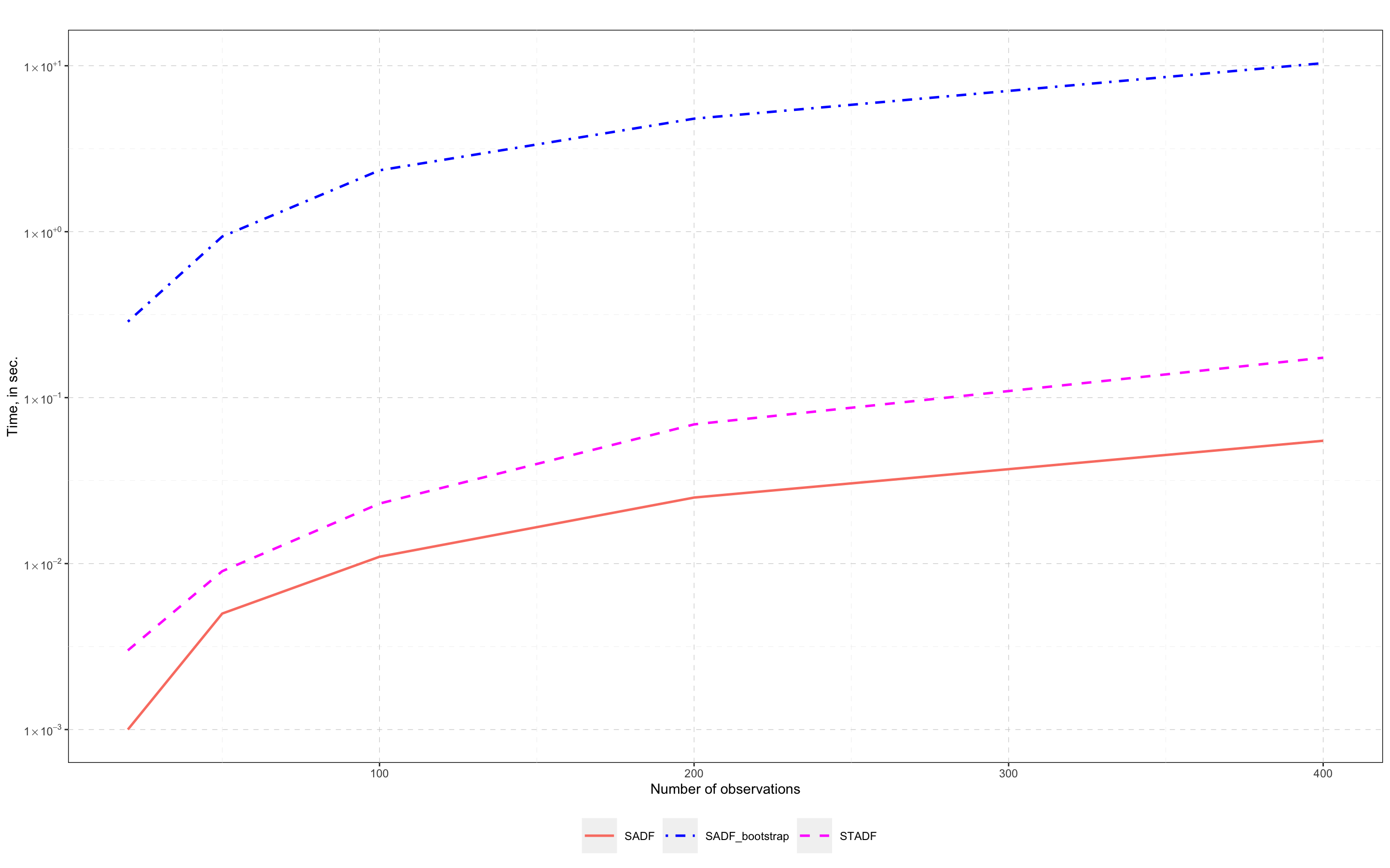
Figure 1: Computational time of $SADF$, $SADF_{b}$ and $STADF$ tests

Figure 1 demonstrates the comparative computation time of the $SADF$, $SADF_{b}$, and $STADF$ tests. For the simulation, we used a simple random walk process without bubbles or volatility shifts. We estimated the median computation time for 1000 iterations and for 20, 50, 100, 200 and 400 observations. For $SADF_{b}$, we used $B=199$. It should be noted that the computation times of the $STADF$ and $SADF_{b}$ tests differ dozens of times. For example, for $T=400$, the median computation time of the $STADF$ test was 0.17 seconds, and the running time of the $SADF_{b}$ was 10.37 seconds, a difference of more than 59 times. At the same time, $STADF$ test is slightly slower than the $SADF$ test, which is to be expected.

6 Empirical application

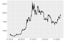
(a) btc

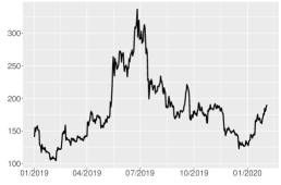
(b) eth

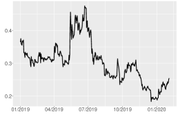
(c) xrp

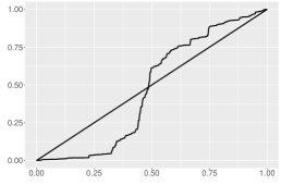
(d) $\eta_{btc}$

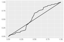
(e) $\eta_{eth}$

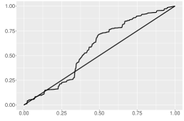
(f) $\eta_{xrp}$

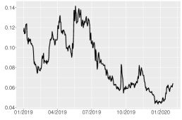
(g) xlm

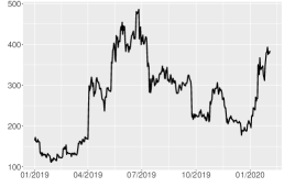
(h) bch

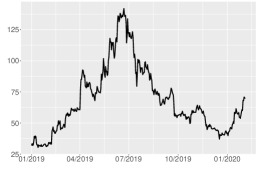
(i) ltc

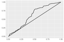
(j) $\eta_{xlm}$

(k) $\eta_{bch}$

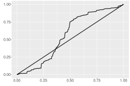
(l) $\eta_{ltc}$

Figure 2: Time series plot of btc, eth, xrp, xlm, bch, ltc and corresponding variance profiles

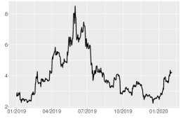
(a) eos

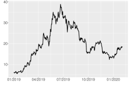
(b) bnb

(c) ada

(d) $\eta_{eos}$

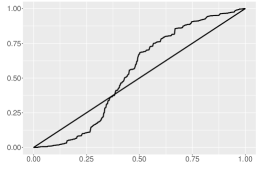
(e) $\eta_{bnb}$

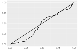
(f) $\eta_{ada}$

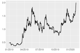
(g) xtz

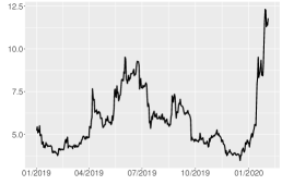
(h) etc

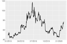
(i) xmr

(j) $\eta_{xtz}$

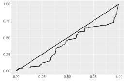
(k) $\eta_{etc}$

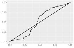
(l) $\eta_{xmr}$

Figure 3: Time series plot of eos, bnb, ada, xtz, etc, xmr and corresponding variance profiles

In this section, we investigate whether or not we observe the emergence of a bubble in the top 12 largest cryptocurrencies by capitalization as of February 3, 2020 (btc, eth, xrp, xlm, bch, ltc, eos, bnb, ada, xtz, etc, xmr), from January 1, 2019 to February 3, 2020, which were 399 observations. In all cases, the closing price in US dollars at 00:00 GMT on the corresponding day is used. The time series with corresponding estimated variance profiles are plotted in Figures 2 and 3. For comparative analysis, we use the same tests as in the previous section: the standard $SADF$ test, the wild bootstrap $SADF$ test ($SADF_{b}$), a union of rejections of the $SADF_{b}$ and SBZ tests ($SBZ$), a union of rejections of the $SADF_{b}$ and sign-based tests ($sSADF$) and the $STADF$ test. For the wild bootstrap $p$-values, $B=999$ bootstrap replications were used. For the standard $SADF$ test and the time-transformed test $STADF$, the $p$-values are obtained by simulations of the asymptotic distributions of the test statistics under homoskedasticity. Table 7 presents the results of the tests (p-values) for the time series considered. We use $r_{0}=0.1$ for ease of calculations of the p-values; the overall tendency will be the same even if we use $r_{0}=\lfloor 0.01+1.8/\sqrt{T}\rfloor$.

From Table 7, we observe several patterns of the $p$-values. For btc and ada series, the $SADF$ strongly rejects the null hypothesis and the other robust tests also reject the null but with larger $p$-values. This implies that we observe a bubble in this period for btc and ada series but the upsurge behaviour in the sample is partially explained by the volatility change. For eth, bch, ltc, eos, bnb, xtz and etc series, the p-values of the SADF test is below 0.05 or 0.1 but the other robust tests, except for $SADF_{b}$ for eth, bch and xtz and $SBZ$ for bnb and xtz, do not reject the null hypothesis at the 10% level. Note that the variance profiles of these series show that there exist some regimes in which volatility moves from low to high. In this case, the SADF test suffers from strong over-rejection and also the $SADF_{b}$ and $SBZ$ tests tend to be mildly over-sized as is observed in the simulation section. By taking this into account, we should not reject the null hypothesis and there is no strong evidence of the existence of a bubble for these series. Finally, for xrp, xlm and xmr series, we do not observe the existence of a bubble by all the tests.

As demonstrated above, we should carefully interpret the empirical results of the tests for a bubble using the estimated variance profile. If we observe a regime with the upward volatility shift, the standard test as well as some of the robust tests tend to over-reject the null hypothesis. The inspection of the combination of the bubble tests and the variance profile will lead us to a more reliable result.

Finally, Table 8 demonstrates the computation time of $SADF$, $SADF_{b}$ and $STADF$ for long time series with thousands observations. It can be seen that the bootstrap based $SADF_{b}$ test is much more computationally expensive in comparison to our proposed $STADF$. At the same time, the statistical conclusions based on the $STADF$ and $SADF_{b}$ tests do not contradict each other for all time series and for the significance level of 5%, which indicates the obvious advantage of the $STADF$ test.

7 Conclusion

In this paper, we proposed the test for bubbles under non-stationary volatility, which includes a finite number of jumps and a nonlinear shift of volatility. Our test is based on the sup-type $t$-statistics expanded under the null hypothesis, using the time-transformed data based on the variance profile. Due to this time-deformation technique, which was proposed by Cavaliere and Taylor, 2007b , we can treat the newly sampled data as if they were generated from the innovations with a constant variance. In fact, we showed that our test is asymptotically free of nuisance parameters and thus it can be conducted by using the asymptotic critical values. This implies that our test is computationally less expensive than the other existing bootstrap based tests in the literature. The finite sample performance showed that we can control the empirical size of our test relatively well and that our test performs better than the other existing tests robust to non-stationary volatility in view of power in some cases, although this is not always the case and it is less powerful in some other cases. Therefore, none of the existing tests outperforms the others uniformly. In this sense, our test can complement the existing ones and is useful to investigate the existence of a bubble under non-stationary volatility. In addition, our empirical example with the cryptocurrencies showed that the volatile behaviour of the time series can be partly explained by volatility changes and thus it is important to take volatility changes into account for such series.

Appendix A Appendix: Proofs

In this appendix, we denote C a generic constant that may differ from place to place. Also, because we subtract the initial value from all the observations, we set $y_{0}=0$ without loss of generality.

Let $T_{1,0}\coloneqq[\tau_{1,0}T]$, $T_{2,0}\coloneqq[\tau_{2,0}T]$ and $T_{3,0}\coloneqq[\tau_{3,0}T]$ and decompose the sample period such that $B_{0}\coloneqq[1,Th]$, $A_{1}\coloneqq[Th+1,T_{1,0}-Th]$, $B_{1}\coloneqq[T_{1,0}-Th+1,T_{1,0}+Th]$, $A_{2}\coloneqq[T_{1,0}+Th+1,T_{2,0}-Th]$, $B_{2}\coloneqq[T_{2,0}-Th+1,T_{2,0}+Th]$, $A_{3}\coloneqq[T_{2,0}+Th+1,T_{3,0}-Th]$, $B_{3}\coloneqq[T_{3,0}-Th+1,T_{3,0}+Th]$, $A_{4}\coloneqq[T_{3,0}+Th+1,T-Th]$, and $B_{4}\coloneqq[T-Th+1,T]$. We first state the asymptotic order of $\hat{\delta}_{t}$ given by (18), which is derived in Lemma 1 of Harvey et al., (2021). Note that Harvey et al., (2021) assumed the continuity of $\sigma_{t}$ throughout their paper, but this assumption is not used as far as the derivation of the following result is concerned and thus $\sigma_{t}$ can be discontinuous such as having a finite number of jumps.

Lemma 1

Let $\phi_{1}=1+\delta_{1}$ and $\phi_{2}=1-\delta_{2}$. Under Assumptions 1 and 2,

$$\max_{Th+1\leq t\leq T_{1,0}-Th}|\hat{\delta}_{t}-\delta_{t}| = O_{p}\left(\sqrt{\frac{\log(T)}{T^{2}h}}\right),$$

$$\max_{T_{1,0}+Th+1\leq t\leq T_{2,0}-Th}|\phi_{1}^{t+Th-1-T_{1,0}}(\hat{\delta}_{t}-\delta_{t})| = O_{p}\left(\frac{\log^{2}(T)}{T^{1/2-1/p}}\right),$$

$$\max_{T_{2,0}+Th+1\leq t\leq T_{3,0}-Th}|\phi_{2}^{t-Th-1-T_{2,0}}(\hat{\delta}_{t}-\delta_{t})| = O_{p}\left(\frac{\log^{2}(T)}{\phi_{1}^{T_{2,0}-T_{1,0}}T^{1/2-1/p}}\right),$$

$$\max_{T_{3,0}+Th+1\leq t\leq T-Th}|\hat{\delta}_{t}-\delta_{t}| = O_{p}\left(\sqrt{\frac{\log(T)}{(a_{T}\vee\sqrt{T})^{2}Th}}\right).$$

The next lemma is concerned with the order of $y_{t}$, which is derived by using Lemma 1.

Lemma 2

Under Assumption 1,

$$y_{t}=\left\{\begin{array}[]{lcl}O_{p}(\sqrt{T})&:&1\leq t\leq T_{1,0}\\ \phi_{1}^{t-T_{1,0}}O_{p}(\sqrt{T})&:&T_{1,0}+1\leq t\leq T_{2,0}\\ \phi_{2}^{t-T_{2,0}}\phi_{1}^{T_{2,0}-T_{1,0}}O_{p}(\sqrt{T})&:&T_{2,0}+1\leq t<T_{3,0}\\ O_{p}(a_{T}\vee\sqrt{T})&:&T_{3,0}+1\leq t\leq T\end{array}\right.$$

where the orders are uniform over the corresponding range of $t$.

Proof: For $1\leq t\leq T_{1,0}$, we have

$$y_{t}=y_{0}+\sum_{j=1}^{t}\varepsilon_{t}$$

and thus, we obtain the result by (5).

For $T_{1,0}+1\leq t\leq T_{2,0}$, we can recursively solve $y_{t}$ as

$$y_{t}=\phi_{1}^{t-T_{1,0}}\left(y_{T_{1,0}}+\sum_{j=T_{1,0}+1}^{t}\phi_{1}^{T_{1,0}-j}\varepsilon_{j}\right).$$

Using Hajék-Rényi inequality for martingale differences, we have

$$P\left(\max_{T_{1,0}+1\leq t\leq T_{2,0}}\left|\sum_{j=T_{1,0}+1}^{t}\phi_{1}^{T_{1,0}-j}\varepsilon_{j}\right|\geq M\right) \leq \frac{1}{M^{2}}\sum_{j=T_{1,0}+1}^{T_{2,0}}\phi_{1}^{2(T_{1,0}-j)}\sigma_{j}^{2}$$

$$\leq \frac{C}{M^{2}}\frac{1-\phi_{1}^{-2(T_{2,0}-T_{1,0})}}{\phi_{1}^{2}-1}<\frac{C}{M^{2}}$$

and thus $\max_{T_{1,0}+1\leq t\leq T_{2,0}}\left|\sum_{j=T_{1,0}+1}^{t}\phi_{1}^{T_{1,0}-j}\varepsilon_{j}\right|=O_{p}(1)$. Since $y_{T_{1,0}}=O_{p}(\sqrt{T})$, we have

$$y_{t}=\phi_{1}^{t-T_{1,0}}(O_{p}(\sqrt{T})+O_{p}(1))$$

uniformly. In particular, we have $y_{T_{2,0}}=\phi_{1}^{T_{2,0}-T_{1,0}}O_{p}(\sqrt{T})$.

Similarly, for $T_{2,0}+1\leq t<T_{3,0}$, we have

$$y_{t}=\phi_{2}^{t-T_{2,0}}y_{T_{2,0}}+\sum_{j=T_{2,0}+1}^{t}\phi_{2}^{t-j}\varepsilon_{j},$$

where the second term on the right-hand side can be shown to be $O_{p}(1)$ uniformly because $|\phi_{2}|<1$. Using the above result, we have $y_{t}=\phi_{2}^{t-T_{2,0}}\phi_{1}^{T_{2,0}-T_{1,0}}O_{p}(\sqrt{T})+O_{p}(1)$.

For $T_{3,0}\leq t\leq T$, $y_{t}=y_{T_{3,0}}+\sum_{j=T_{3,0}+1}^{t}\varepsilon_{t}$ and, using the assumption for $y_{T_{3,0}}$, we obtain the result.$\blacksquare$

Proof of Theorem 1: (i) is obtained from (11)–(13) and (16).

(ii) To show the consistency, it is sufficient to show that $TADF_{r_{1}}^{r_{2}}$ given in (17) goes to infinity for a given specific value of $r_{1}$ and $r_{2}$. In particular, we consider the case where $r_{1}<\eta(\tau_{1,0})<\eta(\tau_{2,0})=r_{2}$, which is equivalent to $g(r_{1})<\tau_{1,0}<\tau_{2,0}=g(r_{2})$.

For the numerator, we can see from Lemma 2 that

$$\tilde{y}_{\lfloor r_{2}T\rfloor}^{2}-\tilde{y}_{\lfloor r_{1}T\rfloor}^{2}-\bar{\omega}^{2}(\lfloor r_{2}T\rfloor-\lfloor r_{1}T\rfloor) = {y}_{\lfloor\tau_{2,0}T\rfloor}^{2}-{y}_{\lfloor g(\lfloor r_{1}T\rfloor/T)T\rfloor}^{2}-\bar{\omega}^{2}(\lfloor r_{2}T\rfloor-\lfloor r_{1}T\rfloor)$$ (A.1)

$$= O_{p}\left(T\phi_{1}^{2(T_{2,0}-T_{1,0})}\right)-O_{p}(T)-O_{p}(T)$$

$$= O_{p}\left(T\phi_{1}^{2(T_{2,0}-T_{1,0})}\right),$$

where the dominant term is positive.

On the other hand, we rewrite the summation in the numerator with respect to the original time ordering such that

$$\sum_{t=\lfloor r_{1}T\rfloor+1}^{\lfloor r_{2}T\rfloor}\tilde{y}_{t-1}^{2}=\sum_{t=\lfloor r_{1}T\rfloor+1}^{\lfloor r_{2}T\rfloor}y_{\lfloor g((t-1)/T)T\rfloor}^{2}.$$

Note that the summation is taken from $t=\lfloor r_{1}T\rfloor+1$ to $\lfloor r_{2}T\rfloor$ and thus the total number of summands is $\lfloor r_{2}T\rfloor-\lfloor r_{1}T\rfloor$, but, as we can see by focusing on the index given by $\lfloor g((t-1)/T)T\rfloor$, some of the original observations between $t=\lfloor g(\lfloor r_{1}T\rfloor/T)T\rfloor$, $\lfloor g(\lfloor r_{1}T\rfloor/T)T\rfloor+1,\ldots,\lfloor g((\lfloor r_{2}T\rfloor-1)/T)T\rfloor$ may not appear as summands whereas the others may be summed up a few times. In particular, some of the non-time-transformed observations in the law volatility regime may be skipped but those in the high volatility regime may be added several times (but finite times). Taking this into account, we can see that for some constant $C$,

$$\sum_{t=\lfloor r_{1}T\rfloor+1}^{\lfloor r_{2}T\rfloor}\tilde{y}_{t-1}^{2} \leq C\sum_{t=\lfloor g(\lfloor r_{1}T\rfloor/T)T\rfloor}^{\lfloor g(\lfloor r_{2}T\rfloor/T)T\rfloor}y_{t}^{2}$$

$$= C\sum_{t=\lfloor g(\lfloor r_{1}T\rfloor/T)T\rfloor}^{\lfloor\tau_{1,0}T\rfloor}y_{t}^{2}+C\sum_{t=\lfloor\tau_{1,0}T\rfloor+1}^{\lfloor\tau_{2,0}T\rfloor}y_{t}^{2}$$

$$= O_{p}(T^{2})+O_{p}\left(T\phi_{1}^{2(T_{2,0}-T_{1,0})}\right)=O_{p}\left(T\phi_{1}^{2(T_{2,0}-T_{1,0})}\right),$$

where the orders are obtained by using Lemma 2. By combining this with (A.1), we can finally have

$$TADF_{r_{1}}^{r_{2}}=O_{p}\left(\sqrt{T}\phi_{1}^{T_{2,0}-T_{1,0}}\right)$$

and the dominant term is positive.$\blacksquare$

Proof of Proposition 2: (i) As explained in the proof of Theorem 2 of Cavaliere and Taylor, 2007a , it is sufficient to prove the pointwise convergence. They showed that $\tilde{\eta}(s)\stackrel{{\scriptstyle p}}{{\longrightarrow}}\eta(s)$ where $\tilde{\eta}(s)$ is defined as $\hat{\eta}(s)$ with $\hat{\varepsilon}_{t}^{*}$ replaced by $\varepsilon_{t}$. Then, the rest we have to show is the pointwise convergence given by

$$\left|\frac{1}{T}\sum_{t=1}^{\lfloor sT\rfloor}\hat{\varepsilon}_{t}^{*2}-\frac{1}{T}\sum_{t=1}^{\lfloor sT\rfloor}\varepsilon_{t}^{2}\right|\stackrel{{\scriptstyle p}}{{\longrightarrow}}0.$$ (A.2)

Let ${\cal A}=A_{1}\cup A_{2}\cup A_{3}\cup A_{4}$ and ${\cal B}=B_{0}\cup B_{1}\cup B_{2}\cup B_{3}\cup B_{4}$. We consider (A.2) on ${\cal A}$ and ${\cal B}$ separately. For brevity of notation, we write $t\in[1,\lfloor sT\rfloor]\cap{\cal A}$ as $t\in{\cal A}$ and $t\in[1,\lfloor sT\rfloor]\cap{\cal B}$ as $t\in{\cal B}$, respectively.

To show (A.2) on ${\cal A}$, we first note that, because $\hat{\varepsilon}_{t}=-(\hat{\delta}_{t}-\delta_{t})y_{t-1}+\varepsilon_{t}$,

$$\frac{1}{T}\sum_{t\in{\cal A}}\hat{\varepsilon}_{t}^{*2} = \frac{1}{T}\sum_{t\in{\cal A}}(\hat{\delta}_{t}-\delta_{t})^{2}y_{t-1}^{2}1(|\hat{\varepsilon}_{t}|<\psi_{T})$$

$$-\frac{2}{T}\sum_{t\in{\cal A}}(\hat{\delta}_{t}-\delta_{t})y_{t-1}\varepsilon_{t}1(|\hat{\varepsilon}_{t}|<\psi_{T})+\frac{1}{T}\sum_{t\in{\cal A}}\varepsilon_{t}^{2}1(|\hat{\varepsilon}_{t}|<\psi_{T})$$

$$= I+II+III.$$

We will show that $I\stackrel{{\scriptstyle p}}{{\longrightarrow}}0$ and $II\stackrel{{\scriptstyle p}}{{\longrightarrow}}0$, while $III-T^{-1}\sum\varepsilon_{t}^{2}\stackrel{{\scriptstyle p}}{{\longrightarrow}}0$.

To show $I\stackrel{{\scriptstyle p}}{{\longrightarrow}}0$, it is sufficient to show that

$$\left|I\right|\leq\frac{1}{T}\sum_{t\in{\cal A}}(\hat{\delta}_{t}-\delta_{t})^{2}y_{t-1}^{2}\stackrel{{\scriptstyle p}}{{\longrightarrow}}0.$$ (A.3)

Using Lemmas 1 and 2, we have

$$\max_{t\in A_{1}}\frac{1}{T}\sum_{i=Th+1}^{t}(\hat{\delta}_{i}-\delta_{i})^{2}y_{i-1}^{2}=O_{p}\left(\frac{\log(T)}{T^{2}h}\right)O_{p}(T)=O_{p}\left(\frac{\log(T)}{Th}\right)=o_{p}(1),$$

$$\max_{t\in A_{2}}\frac{1}{T}\sum_{i=T_{1,0}+Th+1}^{t}(\hat{\delta}_{i}-\delta_{i})^{2}y_{i-1}^{2} = \max_{t\in A_{2}}\frac{1}{T}\sum_{i=T_{1,0}+Th+1}^{t}\phi_{1}^{2(i+Th-1-T_{1,0})}(\hat{\delta}_{i}-\delta_{i})^{2}\phi_{1}^{-2(i-T_{1,0})}y_{i-1}^{2}\phi_{1}^{-2(Th-1)}$$

$$= O_{p}\left(\frac{\log^{4}(T)}{T^{1-2/p}}\right)O_{p}(T)\phi_{1}^{-2(Th-1)}$$

$$= O_{p}\left(\frac{T^{2/p}\log^{4}(T)}{\phi_{1}^{2(Th-1)}}\right)=o_{p}(1),$$

$$\max_{t\in A_{3}}\frac{1}{T}\sum_{i=T_{2,0}+Th+1}^{t}(\hat{\delta}_{i}-\delta_{i})^{2}y_{i-1}^{2} = \max_{t\in A_{3}}\frac{1}{T}\sum_{i=T_{2,0}+Th+1}^{t}\phi_{2}^{2(i-Th-1-T_{2,0})}(\hat{\delta}_{i}-\delta_{i})^{2}\phi_{2}^{-2(i-T_{2,0})}y_{i-1}^{2}\phi_{2}^{2(Th+1)}$$

$$= O_{p}\left(\frac{\log^{4}(T)}{\phi_{1}^{2(T_{2,0}-T_{1,0})}T^{1-2/p}}\right)O_{p}\left(\phi_{1}^{2(T_{2,0}-T_{1,0})}T\right)\phi_{2}^{2(Th+1)}$$

$$= O_{p}\left(\phi_{2}^{2(Th+1)}T^{2/p}\log^{4}(T)\right)=o_{p}(1),$$

$$\max_{t\in A_{4}}\frac{1}{T}\sum_{i=T_{3,0}+Th+1}^{t}(\hat{\delta}_{i}-\delta_{i})^{2}y_{i-1}^{2}=O_{p}\left(\frac{\log(T)}{(a_{T}\vee\sqrt{T})^{2}Th}\right)O_{p}\left((a_{T}\vee\sqrt{T})^{2}\right)=O_{p}\left(\frac{\log(T)}{Th}\right)=o_{p}(1).$$

These results imply (A.3).

For $III$, we have

$$\frac{1}{T}\sum_{t\in{\cal A}}\varepsilon_{t}^{2}1\left(|\hat{\varepsilon}_{t}|<\psi_{T}\right)-\frac{1}{T}\sum_{t\in{\cal A}}\varepsilon_{t}^{2} = \frac{1}{T}\sum_{t\in{\cal A}}\varepsilon_{t}^{2}1\left(|\hat{\varepsilon}_{t}|\geq\psi_{T}\right)$$

$$\leq 1\left(\max_{t\in{\cal A}}|\hat{\varepsilon}_{t}|\geq\psi_{T}\right)\frac{1}{T}\sum_{t\in{\cal A}}\varepsilon_{t}^{2},$$

and thus, it is sufficient to show that

$$1\left(\max_{t\in{\cal A}}|\hat{\varepsilon}_{t}|\geq\psi_{T}\right)=o_{p}(1).$$ (A.4)

Note that $\hat{\varepsilon}_{t}=-(\hat{\delta}_{t}-\delta_{t})y_{t-1}+\varepsilon_{t}$. Similarly to the proof of the convergence of the term $I$, the first term on the right-hand side can be shown to be $o_{p}(1)$ uniformly over ${t\in{\cal A}}$ by using Lemmas 1 and 2, while

$$P\left(\max_{t\in{\cal A}}|\varepsilon_{t}|\geq\psi_{T}\right) \leq \sum_{t\in{\cal A}}P\left(|\varepsilon_{t}|\geq\psi_{T}\right)$$

$$\leq \frac{1}{\psi_{T}^{p}}\sum_{t\in{\cal A}}E|\varepsilon_{t}|^{p}$$

$$\leq C\frac{T}{\psi_{T}^{p}}.$$

Because $T/\psi_{T}^{p}\to 0$ by Assumption 3(b), (A.4) holds.

The convergence of $II$ is obtained by using (A.3), by noting that

$$|II| \leq \frac{2}{T}\sum_{t\in{\cal A}}\left|(\hat{\delta}_{t}-\delta_{t})y_{t-1}\varepsilon_{t}\right|1\left(|\hat{\varepsilon}_{t}|<\psi_{T}\right)$$

$$\leq 2\sqrt{\frac{1}{T}\sum_{t\in{\cal A}}(\hat{\delta}_{t}-\delta_{t})^{2}y_{t-1}^{2}}\sqrt{\frac{1}{T}\sum_{t\in{\cal A}}\varepsilon_{t}^{2}}$$

$$= o_{p}(1).$$

To see (A.2) on ${\cal B}$, we show that each term in (A.2) converges to zero in probability on ${\cal B}$. Because the number of the observations on ${\cal B}$ is proportional to $Th$, we have

$$\frac{1}{T}\sum_{t\in{\cal B}}\hat{\varepsilon}_{t}^{*2}=\frac{1}{T}\sum_{t\in{\cal B}}\hat{\varepsilon}_{t}^{2}1\left(|\hat{\varepsilon}_{t}|<\psi_{T}\right)\\ \leq C\frac{Th}{T}\psi_{T}^{2}=O(h\psi_{T}^{2})=o(1),$$

by Assumption 3. Similarly, we can see that on $t\in{\cal B}$,

$$\frac{1}{T}\sum_{t\in{\cal B}}\varepsilon_{t}^{2}=O_{p}(h)=o_{p}(1).$$

We then obtain (A.2) on ${\cal B}$.

(ii) As discussed in Cavaliere and Taylor, 2007b , the result (i) implies the uniform convergence of $\hat{g}(s)$ to $g(s)$. Thus, following Theorem 1 of Cavaliere and Taylor, 2007b , we have

$$\frac{1}{\sqrt{T}}y_{\lfloor\hat{g}(s)T\rfloor}\Rightarrow\bar{\omega}W(s).\blacksquare$$

Table 1: Finite sample sizes and powers of nominal 0.05-level tests, single volatility shift, $\tau=0.5$

$\sigma_{1}/\sigma_{0}$	$\delta_{1}$	$SADF$	$SADF_{b}$	$SBZ$	$sSADF$	$sSADF_{u}$	$STADF$	$SADF$	$SADF_{b}$	$SBZ$	$sSADF$	$sSADF_{u}$	$STADF$
		$T=100$						$T=200$
$1/6$	0.00	0.012	0.027	0.065	0.043	0.033	0.059	0.029	0.047	0.081	0.037	0.050	0.040
	0.02	0.022	0.047	0.112	0.204	0.173	0.135	0.110	0.149	0.254	0.536	0.509	0.328
	0.04	0.099	0.164	0.254	0.375	0.348	0.301	0.587	0.615	0.638	0.753	0.747	0.664
	0.06	0.352	0.392	0.455	0.497	0.496	0.500	0.843	0.861	0.862	0.861	0.888	0.855
	0.08	0.566	0.608	0.628	0.556	0.637	0.642	0.933	0.935	0.936	0.923	0.950	0.929
	0.10	0.728	0.743	0.753	0.631	0.759	0.744	0.961	0.964	0.964	0.939	0.970	0.953
$1/3$	0.00	0.015	0.039	0.065	0.036	0.038	0.036	0.025	0.036	0.062	0.039	0.030	0.048
	0.02	0.027	0.056	0.114	0.129	0.118	0.135	0.127	0.178	0.262	0.379	0.349	0.331
	0.04	0.112	0.166	0.275	0.301	0.293	0.327	0.581	0.610	0.628	0.668	0.677	0.652
	0.06	0.335	0.384	0.435	0.428	0.436	0.487	0.841	0.847	0.848	0.834	0.865	0.852
	0.08	0.597	0.632	0.653	0.559	0.649	0.662	0.921	0.924	0.926	0.885	0.932	0.925
	0.10	0.729	0.757	0.770	0.623	0.753	0.748	0.971	0.973	0.973	0.939	0.972	0.968
1	0.00	0.022	0.032	0.064	0.039	0.038	0.047	0.033	0.039	0.067	0.042	0.043	0.049
	0.02	0.067	0.072	0.143	0.077	0.083	0.114	0.212	0.234	0.313	0.180	0.237	0.285
	0.04	0.202	0.219	0.312	0.181	0.228	0.264	0.605	0.615	0.639	0.476	0.604	0.595
	0.06	0.419	0.418	0.482	0.297	0.406	0.442	0.847	0.842	0.843	0.723	0.838	0.819
	0.08	0.615	0.630	0.663	0.464	0.608	0.625	0.936	0.939	0.940	0.839	0.938	0.926
	0.10	0.711	0.718	0.732	0.540	0.701	0.699	0.969	0.969	0.969	0.902	0.970	0.956
3	0.00	0.284	0.057	0.077	0.040	0.072	0.051	0.366	0.063	0.090	0.056	0.076	0.063
	0.02	0.383	0.096	0.128	0.065	0.101	0.066	0.509	0.173	0.221	0.091	0.171	0.153
	0.04	0.470	0.182	0.228	0.101	0.165	0.161	0.718	0.441	0.485	0.296	0.440	0.406
	0.06	0.594	0.298	0.327	0.170	0.281	0.241	0.864	0.734	0.748	0.552	0.705	0.683
	0.08	0.699	0.459	0.485	0.295	0.429	0.365	0.940	0.873	0.876	0.754	0.860	0.845
	0.10	0.790	0.630	0.656	0.402	0.610	0.526	0.962	0.928	0.928	0.831	0.921	0.904
6	0.00	0.540	0.084	0.101	0.049	0.079	0.045	0.608	0.070	0.094	0.037	0.067	0.061
	0.02	0.586	0.114	0.130	0.053	0.095	0.056	0.691	0.136	0.172	0.082	0.140	0.089
	0.04	0.632	0.171	0.194	0.090	0.168	0.080	0.792	0.337	0.374	0.244	0.343	0.219
	0.06	0.720	0.223	0.248	0.145	0.235	0.110	0.913	0.598	0.635	0.463	0.597	0.488
	0.08	0.770	0.350	0.375	0.232	0.334	0.174	0.952	0.777	0.796	0.650	0.759	0.703
	0.10	0.844	0.449	0.472	0.293	0.416	0.256	0.976	0.890	0.903	0.788	0.881	0.859

Table 2: Finite sample sizes and powers of nominal 0.05-level tests, single volatility shift, $\tau=0.3$

$\sigma_{1}/\sigma_{0}$	$\delta_{1}$	$SADF$	$SADF_{b}$	$SBZ$	$sSADF$	$sSADF_{u}$	$STADF$	$SADF$	$SADF_{b}$	$SBZ$	$sSADF$	$sSADF_{u}$	$STADF$
		$T=100$						$T=200$
$1/6$	0.00	0.008	0.045	0.088	0.048	0.049	0.066	0.019	0.047	0.083	0.040	0.052	0.044
	0.02	0.006	0.039	0.086	0.302	0.249	0.157	0.027	0.101	0.245	0.634	0.587	0.395
	0.04	0.025	0.122	0.253	0.601	0.530	0.377	0.631	0.693	0.702	0.860	0.852	0.744
	0.06	0.324	0.433	0.480	0.725	0.679	0.560	0.843	0.868	0.870	0.934	0.926	0.863
	0.08	0.598	0.675	0.689	0.805	0.794	0.722	0.931	0.935	0.936	0.958	0.956	0.930
	0.10	0.735	0.794	0.797	0.850	0.854	0.789	0.965	0.968	0.968	0.968	0.978	0.959
$1/3$	0.00	0.012	0.041	0.077	0.035	0.035	0.076	0.012	0.044	0.077	0.034	0.044	0.050
	0.02	0.004	0.029	0.098	0.157	0.123	0.158	0.056	0.136	0.254	0.403	0.358	0.350
	0.04	0.041	0.143	0.267	0.376	0.336	0.356	0.608	0.672	0.685	0.761	0.748	0.707
	0.06	0.338	0.439	0.483	0.576	0.546	0.549	0.836	0.860	0.864	0.887	0.884	0.858
	0.08	0.593	0.680	0.699	0.703	0.723	0.712	0.936	0.940	0.940	0.935	0.946	0.938
	0.10	0.729	0.772	0.776	0.760	0.794	0.765	0.969	0.970	0.970	0.950	0.970	0.963
1	0.00	0.022	0.032	0.064	0.039	0.038	0.047	0.033	0.039	0.067	0.042	0.043	0.049
	0.02	0.067	0.072	0.143	0.077	0.083	0.114	0.212	0.234	0.313	0.180	0.237	0.285
	0.04	0.202	0.219	0.312	0.181	0.228	0.264	0.605	0.615	0.639	0.476	0.604	0.595
	0.06	0.419	0.418	0.482	0.297	0.406	0.442	0.847	0.842	0.843	0.723	0.838	0.819
	0.08	0.615	0.630	0.663	0.464	0.608	0.625	0.936	0.939	0.940	0.839	0.938	0.926
	0.10	0.711	0.718	0.732	0.540	0.701	0.699	0.969	0.969	0.969	0.902	0.970	0.956
3	0.00	0.316	0.065	0.093	0.044	0.067	0.052	0.342	0.062	0.084	0.035	0.054	0.046
	0.02	0.378	0.098	0.141	0.057	0.105	0.116	0.523	0.157	0.245	0.106	0.163	0.215
	0.04	0.483	0.147	0.220	0.096	0.150	0.202	0.721	0.448	0.519	0.317	0.434	0.525
	0.06	0.599	0.294	0.378	0.193	0.294	0.353	0.859	0.753	0.772	0.584	0.746	0.768
	0.08	0.710	0.464	0.529	0.313	0.447	0.513	0.919	0.879	0.883	0.751	0.870	0.875
	0.10	0.797	0.626	0.679	0.408	0.593	0.651	0.966	0.945	0.947	0.848	0.943	0.945
6	0.00	0.523	0.069	0.087	0.045	0.071	0.045	0.607	0.097	0.117	0.046	0.093	0.057
	0.02	0.556	0.094	0.133	0.054	0.083	0.100	0.702	0.125	0.237	0.108	0.125	0.223
	0.04	0.663	0.119	0.208	0.078	0.130	0.202	0.816	0.358	0.520	0.310	0.374	0.537
	0.06	0.708	0.193	0.331	0.169	0.215	0.334	0.906	0.668	0.752	0.537	0.657	0.765
	0.08	0.775	0.330	0.484	0.263	0.341	0.490	0.936	0.826	0.849	0.699	0.820	0.850
	0.10	0.847	0.509	0.621	0.357	0.496	0.616	0.974	0.934	0.940	0.829	0.934	0.938

Table 3: Finite sample sizes and powers of nominal 0.05-level tests, single volatility shift, $\tau=0.7$

$\sigma_{1}/\sigma_{0}$	$\delta_{1}$	$SADF$	$SADF_{b}$	$SBZ$	$sSADF$	$sSADF_{u}$	$STADF$	$SADF$	$SADF_{b}$	$SBZ$	$sSADF$	$sSADF_{u}$	$STADF$
		$T=100$						$T=200$
$1/6$	0.000	0.026	0.036	0.071	0.045	0.045	0.058	0.037	0.047	0.080	0.042	0.048	0.048
	0.020	0.049	0.073	0.140	0.063	0.076	0.107	0.190	0.213	0.314	0.170	0.217	0.267
	0.040	0.167	0.211	0.308	0.139	0.191	0.257	0.585	0.606	0.628	0.469	0.588	0.591
	0.060	0.433	0.451	0.513	0.331	0.432	0.453	0.860	0.869	0.869	0.708	0.858	0.832
	0.080	0.580	0.609	0.637	0.428	0.587	0.584	0.940	0.944	0.944	0.855	0.938	0.924
	0.100	0.747	0.756	0.765	0.580	0.748	0.734	0.958	0.959	0.959	0.901	0.960	0.952
$1/3$	0.000	0.024	0.037	0.075	0.030	0.043	0.054	0.035	0.042	0.088	0.045	0.051	0.055
	0.020	0.043	0.070	0.132	0.068	0.077	0.123	0.208	0.236	0.318	0.172	0.222	0.275
	0.040	0.158	0.186	0.281	0.139	0.197	0.241	0.617	0.642	0.663	0.497	0.628	0.623
	0.060	0.369	0.393	0.446	0.290	0.386	0.399	0.832	0.836	0.838	0.727	0.831	0.810
	0.080	0.595	0.610	0.634	0.448	0.588	0.598	0.926	0.931	0.931	0.846	0.928	0.921
	0.100	0.757	0.759	0.764	0.566	0.744	0.719	0.965	0.968	0.968	0.903	0.968	0.954
1	0.000	0.022	0.032	0.064	0.039	0.038	0.047	0.033	0.039	0.067	0.042	0.043	0.049
	0.020	0.067	0.072	0.143	0.077	0.083	0.114	0.212	0.234	0.313	0.180	0.237	0.285
	0.040	0.202	0.219	0.312	0.181	0.228	0.264	0.605	0.615	0.639	0.476	0.604	0.595
	0.060	0.419	0.418	0.482	0.297	0.406	0.442	0.847	0.842	0.843	0.723	0.838	0.819
	0.080	0.615	0.630	0.663	0.464	0.608	0.625	0.936	0.939	0.940	0.839	0.938	0.926
	0.100	0.711	0.718	0.732	0.540	0.701	0.699	0.969	0.969	0.969	0.902	0.970	0.956
3	0.000	0.256	0.072	0.092	0.037	0.071	0.053	0.294	0.075	0.098	0.030	0.066	0.060
	0.020	0.258	0.060	0.090	0.078	0.089	0.100	0.425	0.094	0.195	0.161	0.155	0.253
	0.040	0.403	0.131	0.204	0.168	0.187	0.238	0.721	0.486	0.541	0.495	0.523	0.610
	0.060	0.534	0.292	0.363	0.296	0.327	0.402	0.890	0.794	0.801	0.740	0.792	0.814
	0.080	0.704	0.522	0.548	0.430	0.512	0.563	0.954	0.923	0.924	0.868	0.917	0.922
	0.100	0.800	0.668	0.680	0.537	0.656	0.663	0.977	0.951	0.953	0.907	0.949	0.955
6	0.000	0.496	0.080	0.099	0.039	0.075	0.070	0.560	0.064	0.088	0.033	0.059	0.053
	0.020	0.521	0.079	0.112	0.071	0.108	0.080	0.619	0.075	0.132	0.172	0.169	0.073
	0.040	0.534	0.077	0.126	0.154	0.156	0.073	0.828	0.367	0.408	0.496	0.496	0.250
	0.060	0.705	0.169	0.222	0.304	0.300	0.110	0.936	0.710	0.730	0.730	0.751	0.555
	0.080	0.788	0.389	0.424	0.437	0.459	0.219	0.975	0.887	0.897	0.860	0.889	0.782
	0.100	0.870	0.559	0.575	0.548	0.588	0.314	0.986	0.953	0.954	0.912	0.949	0.895

Table 4: Finite sample sizes and powers of nominal 0.05-level tests, double volatility shift

$\sigma_{1}/\sigma_{0}$	$\delta_{1}$	$SADF$	$SADF_{b}$	$SBZ$	$sSADF$	$sSADF_{u}$	$STADF$	$SADF$	$SADF_{b}$	$SBZ$	$sSADF$	$sSADF_{u}$	$STADF$
		$T=100$						$T=200$
$1/6$	0.00	0.029	0.035	0.067	0.040	0.046	0.041	0.046	0.048	0.072	0.040	0.053	0.041
	0.02	0.040	0.052	0.127	0.364	0.332	0.178	0.122	0.160	0.287	0.651	0.643	0.377
	0.04	0.143	0.169	0.295	0.623	0.590	0.383	0.648	0.657	0.667	0.875	0.874	0.706
	0.06	0.376	0.419	0.474	0.746	0.719	0.524	0.848	0.852	0.855	0.937	0.934	0.844
	0.08	0.619	0.645	0.671	0.805	0.797	0.683	0.946	0.948	0.949	0.965	0.969	0.940
	0.10	0.762	0.771	0.776	0.831	0.852	0.769	0.974	0.974	0.974	0.982	0.984	0.969
$1/3$	0.00	0.019	0.027	0.064	0.033	0.035	0.047	0.035	0.042	0.079	0.041	0.047	0.051
	0.02	0.030	0.042	0.137	0.196	0.182	0.162	0.147	0.172	0.303	0.469	0.457	0.362
	0.04	0.117	0.169	0.306	0.441	0.412	0.364	0.652	0.662	0.679	0.763	0.758	0.697
	0.06	0.399	0.430	0.486	0.606	0.595	0.527	0.863	0.866	0.871	0.896	0.903	0.865
	0.08	0.629	0.649	0.667	0.709	0.715	0.675	0.939	0.942	0.944	0.946	0.954	0.929
	0.10	0.762	0.789	0.795	0.783	0.815	0.775	0.975	0.977	0.977	0.961	0.976	0.969
1	0.00	0.022	0.032	0.064	0.039	0.038	0.047	0.033	0.039	0.067	0.042	0.043	0.049
	0.02	0.067	0.072	0.143	0.077	0.083	0.114	0.212	0.234	0.313	0.180	0.237	0.285
	0.04	0.202	0.219	0.312	0.181	0.228	0.264	0.605	0.615	0.639	0.476	0.604	0.595
	0.06	0.419	0.418	0.482	0.297	0.406	0.442	0.847	0.842	0.843	0.723	0.838	0.819
	0.08	0.615	0.630	0.663	0.464	0.608	0.625	0.936	0.939	0.940	0.839	0.938	0.926
	0.10	0.711	0.718	0.732	0.540	0.701	0.699	0.969	0.969	0.969	0.902	0.970	0.956
3	0.00	0.228	0.075	0.087	0.033	0.075	0.063	0.304	0.082	0.099	0.039	0.077	0.062
	0.02	0.318	0.117	0.150	0.053	0.110	0.108	0.460	0.200	0.257	0.090	0.187	0.193
	0.04	0.411	0.200	0.242	0.073	0.176	0.185	0.623	0.438	0.488	0.237	0.399	0.425
	0.06	0.525	0.301	0.364	0.144	0.270	0.323	0.808	0.711	0.734	0.507	0.688	0.710
	0.08	0.615	0.429	0.495	0.205	0.403	0.435	0.892	0.835	0.850	0.668	0.826	0.834
	0.10	0.713	0.562	0.608	0.305	0.526	0.582	0.944	0.923	0.926	0.785	0.920	0.912
6	0.00	0.448	0.085	0.105	0.040	0.087	0.071	0.537	0.082	0.098	0.047	0.074	0.078
	0.02	0.528	0.126	0.172	0.051	0.121	0.123	0.663	0.149	0.224	0.070	0.132	0.176
	0.04	0.596	0.165	0.224	0.068	0.152	0.208	0.740	0.316	0.431	0.171	0.293	0.377
	0.06	0.636	0.223	0.299	0.097	0.200	0.274	0.836	0.567	0.650	0.401	0.545	0.634
	0.08	0.698	0.295	0.389	0.134	0.265	0.377	0.901	0.751	0.792	0.571	0.744	0.780
	0.10	0.761	0.448	0.527	0.224	0.404	0.487	0.955	0.891	0.905	0.684	0.885	0.907

Table 5: Finite sample sizes and powers of nominal 0.05-level tests, logistic smooth transition in volatility

$\sigma_{1}/\sigma_{0}$	$\delta_{1}$	$SADF$	$SADF_{b}$	$SBZ$	$sSADF$	$sSADF_{u}$	$STADF$	$SADF$	$SADF_{b}$	$SBZ$	$sSADF$	$sSADF_{u}$	$STADF$
		$T=100$						$T=200$
$1/6$	0.00	0.021	0.047	0.083	0.043	0.056	0.057	0.026	0.031	0.064	0.046	0.044	0.049
	0.02	0.022	0.058	0.115	0.154	0.138	0.135	0.111	0.157	0.240	0.431	0.400	0.311
	0.04	0.092	0.150	0.254	0.335	0.307	0.323	0.605	0.637	0.665	0.714	0.720	0.690
	0.06	0.341	0.411	0.461	0.464	0.490	0.502	0.842	0.852	0.856	0.858	0.876	0.855
	0.08	0.591	0.642	0.663	0.578	0.653	0.670	0.913	0.922	0.922	0.898	0.933	0.912
	0.10	0.718	0.739	0.747	0.640	0.755	0.738	0.972	0.974	0.974	0.953	0.977	0.971
$1/3$	0.00	0.014	0.034	0.067	0.028	0.040	0.050	0.019	0.038	0.083	0.051	0.051	0.059
	0.02	0.024	0.049	0.115	0.104	0.086	0.139	0.113	0.170	0.272	0.346	0.315	0.335
	0.04	0.114	0.158	0.266	0.263	0.249	0.320	0.605	0.639	0.663	0.678	0.683	0.685
	0.06	0.375	0.447	0.492	0.411	0.470	0.517	0.852	0.865	0.866	0.824	0.875	0.863
	0.08	0.559	0.605	0.635	0.538	0.628	0.639	0.942	0.946	0.946	0.913	0.954	0.944
	0.10	0.728	0.754	0.760	0.611	0.748	0.748	0.967	0.972	0.972	0.924	0.972	0.964
1	0.00	0.022	0.032	0.064	0.039	0.038	0.047	0.033	0.039	0.067	0.042	0.043	0.049
	0.02	0.067	0.072	0.143	0.077	0.083	0.114	0.212	0.234	0.313	0.180	0.237	0.285
	0.04	0.202	0.219	0.312	0.181	0.228	0.264	0.605	0.615	0.639	0.476	0.604	0.595
	0.06	0.419	0.418	0.482	0.297	0.406	0.442	0.847	0.842	0.843	0.723	0.838	0.819
	0.08	0.615	0.630	0.663	0.464	0.608	0.625	0.936	0.939	0.940	0.839	0.938	0.926
	0.10	0.711	0.718	0.732	0.540	0.701	0.699	0.969	0.969	0.969	0.902	0.970	0.956
3	0.00	0.308	0.066	0.089	0.042	0.079	0.050	0.342	0.075	0.095	0.034	0.065	0.051
	0.02	0.379	0.093	0.118	0.052	0.087	0.080	0.496	0.170	0.216	0.100	0.164	0.147
	0.04	0.465	0.185	0.226	0.097	0.172	0.146	0.723	0.480	0.523	0.268	0.448	0.429
	0.06	0.578	0.304	0.354	0.178	0.295	0.240	0.870	0.749	0.761	0.557	0.731	0.696
	0.08	0.700	0.479	0.510	0.264	0.438	0.387	0.920	0.855	0.861	0.691	0.842	0.809
	0.10	0.789	0.630	0.643	0.382	0.600	0.540	0.977	0.954	0.954	0.846	0.944	0.923
6	0.00	0.512	0.073	0.095	0.036	0.072	0.054	0.587	0.082	0.102	0.033	0.070	0.049
	0.02	0.601	0.119	0.144	0.052	0.112	0.074	0.712	0.160	0.198	0.069	0.149	0.110
	0.04	0.641	0.172	0.198	0.075	0.153	0.086	0.792	0.306	0.349	0.175	0.286	0.200
	0.06	0.721	0.247	0.281	0.124	0.227	0.125	0.896	0.605	0.634	0.386	0.578	0.507
	0.08	0.782	0.325	0.364	0.170	0.299	0.168	0.949	0.797	0.811	0.611	0.774	0.731
	0.10	0.840	0.440	0.477	0.270	0.426	0.275	0.973	0.905	0.910	0.766	0.894	0.869

Table 6: Finite sample sizes and powers of nominal 0.05-level tests, trending volatility

$\sigma_{1}/\sigma_{0}$	$\delta_{1}$	$SADF$	$SADF_{b}$	$SBZ$	$sSADF$	$sSADF_{u}$	$STADF$	$SADF$	$SADF_{b}$	$SBZ$	$sSADF$	$sSADF_{u}$	$STADF$
		$T=100$						$T=200$
$1/6$	0.00	0.002	0.032	0.061	0.027	0.037	0.053	0.005	0.037	0.075	0.035	0.041	0.054
	0.02	0.012	0.054	0.139	0.097	0.086	0.119	0.087	0.196	0.306	0.229	0.250	0.301
	0.04	0.093	0.197	0.333	0.226	0.238	0.309	0.605	0.658	0.672	0.608	0.660	0.659
	0.06	0.327	0.437	0.511	0.376	0.439	0.480	0.842	0.858	0.861	0.793	0.857	0.844
	0.08	0.602	0.677	0.692	0.558	0.661	0.645	0.929	0.938	0.938	0.888	0.936	0.926
	0.10	0.731	0.782	0.792	0.634	0.777	0.757	0.963	0.970	0.970	0.910	0.967	0.952
$1/3$	0.00	0.009	0.029	0.066	0.026	0.028	0.058	0.008	0.038	0.076	0.035	0.043	0.043
	0.02	0.011	0.056	0.112	0.070	0.068	0.111	0.111	0.201	0.293	0.223	0.234	0.278
	0.04	0.119	0.208	0.323	0.202	0.236	0.291	0.579	0.640	0.656	0.568	0.631	0.630
	0.06	0.383	0.460	0.515	0.388	0.466	0.497	0.822	0.844	0.847	0.773	0.839	0.828
	0.08	0.579	0.630	0.651	0.503	0.621	0.615	0.931	0.940	0.942	0.883	0.941	0.927
	0.10	0.721	0.763	0.770	0.619	0.760	0.729	0.961	0.965	0.965	0.906	0.963	0.956
1	0.00	0.022	0.032	0.064	0.039	0.038	0.047	0.033	0.039	0.067	0.042	0.043	0.049
	0.02	0.067	0.072	0.143	0.077	0.083	0.114	0.212	0.234	0.313	0.180	0.237	0.285
	0.04	0.202	0.219	0.312	0.181	0.228	0.264	0.605	0.615	0.639	0.476	0.604	0.595
	0.06	0.419	0.418	0.482	0.297	0.406	0.442	0.847	0.842	0.843	0.723	0.838	0.819
	0.08	0.615	0.630	0.663	0.464	0.608	0.625	0.936	0.939	0.940	0.839	0.938	0.926
	0.10	0.711	0.718	0.732	0.540	0.701	0.699	0.969	0.969	0.969	0.902	0.970	0.956
3	0.00	0.178	0.046	0.071	0.037	0.050	0.042	0.186	0.050	0.076	0.044	0.059	0.054
	0.02	0.227	0.087	0.133	0.063	0.084	0.100	0.405	0.187	0.270	0.127	0.189	0.239
	0.04	0.358	0.161	0.237	0.122	0.161	0.202	0.687	0.564	0.599	0.380	0.551	0.555
	0.06	0.511	0.357	0.413	0.219	0.341	0.379	0.857	0.801	0.811	0.640	0.787	0.780
	0.08	0.657	0.535	0.571	0.358	0.517	0.525	0.924	0.898	0.901	0.782	0.894	0.884
	0.10	0.738	0.650	0.674	0.455	0.636	0.625	0.958	0.947	0.949	0.862	0.945	0.933
6	0.00	0.291	0.060	0.071	0.038	0.056	0.041	0.340	0.053	0.076	0.032	0.050	0.042
	0.02	0.340	0.077	0.127	0.065	0.079	0.098	0.510	0.175	0.250	0.124	0.169	0.211
	0.04	0.498	0.175	0.241	0.110	0.149	0.186	0.722	0.499	0.542	0.345	0.471	0.502
	0.06	0.551	0.308	0.360	0.175	0.295	0.305	0.874	0.765	0.780	0.578	0.748	0.744
	0.08	0.697	0.492	0.530	0.307	0.461	0.494	0.949	0.901	0.905	0.762	0.895	0.880
	0.10	0.812	0.635	0.668	0.430	0.603	0.610	0.980	0.962	0.963	0.858	0.961	0.950

Table 7: Empirical results, $p$-values

Series	$SADF$	$SADF_{b}$	$SBZ$	$sSADF$	$STADF$
btc	0.000	0.083	0.109	0.093	0.099
eth	0.004	0.081	0.125	0.190	0.486
xrp	0.951	0.936	0.935	0.125	0.915
xlm	0.837	0.753	0.643	0.379	0.335
bch	0.000	0.072	0.109	0.146	0.189
ltc	0.042	0.228	0.252	0.439	0.186
eos	0.093	0.284	0.277	0.656	0.191
bnb	0.013	0.209	0.070	0.414	0.108
ada	0.000	0.046	0.065	0.086	0.044
xtz	0.000	0.059	0.099	0.109	0.373
etc	0.027	0.139	0.234	0.350	0.373
xmr	0.119	0.361	0.398	0.501	0.442

Table 8: Empirical results for large sample sizes, $p$-values and computational time (in seconds)

Series	Start date	End date	$T$	$SADF$		$SADF_{b}$		$STADF$
				time	$p$-value	time	$p$-value	time	$p$-value
btc	2010-07-18	2021-06-01	3972	1.59	0.000	336.31	0.000	6.21	0.044
eth	2015-08-08	2021-06-01	2125	0.48	0.000	104.60	0.000	2.09	0.011
xrp	2014-08-15	2021-06-01	2483	0.63	0.000	133.60	0.000	2.78	0.000
xlm	2015-09-30	2021-06-01	2072	0.44	0.000	91.32	0.000	2.03	0.000
ltc	2013-04-01	2021-06-01	2984	1.00	0.000	213.59	0.000	3.81	0.000

References

- Astill et al., (2021) Astill, S., Harvey, D., Leybourne, S., Taylor, A., and Zu, Y. (2021). CUSUM-based monitoring for explosive episodes in financial data in the presence of time-varying volatility. forthcoming in Journal of Financial Econometrics.
- Cavaliere, (2004) Cavaliere, G. (2004). Unit root tests under time-varying variances. Econometric Reviews, 23:259–292.
- (3) Cavaliere, G. and Taylor, A. M. R. (2007a). Testing for unit roots in time series models with non-stationary volatility. Journal of Econometrics, 140:919–947.
- (4) Cavaliere, G. and Taylor, A. M. R. (2007b). Time-transformed unit root tests for models with non-stationary volatility. Journal of Time Series Analysis, 29:300–330.
- Cavaliere and Taylor, (2008) Cavaliere, G. and Taylor, A. M. R. (2008). Bootstrap unit root tests for time series with nonstationary volatility. Econometric Theory, 24:43–71.
- Hafner, (2020) Hafner, C. (2020). Testing for bubbles in cryptocurrencies with time-varying volatility. Journal of Financial Econometrics, 18(2):233–249.
- Harvey et al., (2016) Harvey, D., Leybourne, S., Sollis, R., and Taylor, A. (2016). Tests for Explosive Financial Bubbles in the Presence of Non-stationary Volatility. Journal of Empirical Finance, 38:548–574.
- Harvey et al., (2019) Harvey, D., Leybourne, S., and Zu, Y. (2019). Tests Explosive Bubbles with Time-varying Volatility. Econometric Reviews, 38:1131–1151.
- Harvey et al., (2020) Harvey, D., Leybourne, S., and Zu, Y. (2020). Sign-based unit root tests for explosive financial bubbles in the presence of deterministically time-varying volatility. Econometric Theory, 36(1):122–169.
- Harvey et al., (2021) Harvey, D., Leybourne, S., and Zu, Y. (2021). Estimation of the variance function in structural break autoregressive models with nonstationary and explosive segments. Unpublished Manuscript.
- Homme and Breitung, (2012) Homme, U. and Breitung, J. (2012). Testing for speculative bubbles in stock markets: A comparison of alternative methods. Journal of Financial Econometrics, 10(1):198–231.
- Karatzas and Shreve, (1991) Karatzas, I. and Shreve, S. (1991). Brownian Motion and Stochastic Clculus Second Edition. Springer, New York.
- Phillips et al., (2014) Phillips, P., Shi, S., and Yu, J. (2014). Specification Sensitivity in Right-tailed Unit Root Testing for Explosive Behavior. Oxford Bulletin of Economics and Statistics, 76:315–333.
- (14) Phillips, P., Shi, S., and Yu, J. (2015a). Testing for Multiple Bubbles: Historical Episodes of Exuberance and Collapse in the S&P 500. International Economic Review, 56:1043–1077.
- (15) Phillips, P., Shi, S., and Yu, J. (2015b). Testing for Multiple Bubbles: Limit Theory of Real-Time Detectors. International Economic Review, 56:1079–1133.
- Phillips et al., (2011) Phillips, P., Wu, Y., and Yu, J. (2011). Explosive Behavior in the 1990s Nasdaq: When Did Exuberance Escalate Asset Values? International Economic Review, 52:201–226.
- Whitehouse, (2019) Whitehouse, E. (2019). Explosive Asset Price Bubble Detection with Unknown Bubble Length and Initial Condition. Oxford Bulletin of Economics and Statsitics, 81:20–41.