Learning Generalized Spatial-Temporal Deep Feature Representation for No-Reference Video Quality Assessment

Abstract

In this work, we propose a no-reference video quality assessment method, aiming to achieve high-generalization capability in cross-content, -resolution and -frame rate quality prediction. In particular, we evaluate the quality of a video by learning effective feature representations in spatial-temporal domain. In the spatial domain, to tackle the resolution and content variations, we impose the Gaussian distribution constraints on the quality features. The unified distribution can significantly reduce the domain gap between different video samples, resulting in more generalized quality feature representation. Along the temporal dimension, inspired by the mechanism of visual perception, we propose a pyramid temporal aggregation module by involving the short-term and long-term memory to aggregate the frame-level quality. Experiments show that our method outperforms the state-of-the-art methods on cross-dataset settings, and achieves comparable performance on intra-dataset configurations, demonstrating the high-generalization capability of the proposed method. The codes are released at https://github.com/Baoliang93/GSTVQA.

I Introduction

There has been an increasing demand for accurately predicting the quality of videos, coinciding with the exponentially growing of video data. In the context of video big data, it becomes extremely difficult and costly to rely solely on human visual system to conduct timely quality assessment. As such, objective video quality assessment (VQA), the goal of which is to design computational models that automatically and accurately predict the perceived quality of videos, has become more prominent. According to the application scenarios regarding the availability of the pristine reference video, the assessment of video quality can be categorized into full-reference VQA (FR-VQA), reduced-reference VQA (RR-VQA) and no-reference VQA (NR-VQA). Despite remarkable progress, the NR-VQA of real-world videos, which has received great interest due to its high practical utility, is still very challenging especially when the videos are acquired, processed and compressed with diverse devices, environments and algorithms.

For NR-VQA, numerous methods have been proposed in the literature, and the majority of them rely on a machine learning pipeline based on the training of quality prediction model with labeled data. Methods relying on handcrafted features [1, 2, 3, 4] and deep learning features [5, 6, 7, 8] have been developed, with the assumption that the training and testing data are drawn from closely aligned feature spaces. However, it is widely acknowledged that different distributions of training and testing data create the risk of poor generalization capability, and as a consequence, inaccurate predictions could be obtained on the videos that hold dramatically different statistics compared to those in the training set. The underlying design principle of the proposed VQA method is learning features with high generalization capability, such that the model is able to deliver high quality prediction accuracy of videos that are not sampled from the domain of the training data. This well aligns real application scenarios when the testing data are unknown. To verify the performance of our method, we conduct experiments on four cross-dataset settings with available databases, including KoNViD-1k [9], LIVE-Qualcomm [10], LIVE-VQC [11] and CVD2014 [12]. Experimental results have demonstrated superior performance of our method over existing state-of-the-art models with a significant margin. The main contributions of this paper are as follows,

• We propose an objective NR-VQA model that is capable of automatically accessing the perceptual quality of videos resulting from different acquisition, processing and compression techniques. The proposed model is driven by learning features that specifically characterize the quality, and is able to deliver high prediction accuracy for videos that hold dramatically different characteristics compared to the training data.

• In the spatial domain, we develop a multi-scale feature extraction scheme to explore the quality features in different scales, and an attention module is further incorporated to adaptively weight the features by their importance. We further unify the quality features of each frame with a Gaussian distribution where the mean and variance of the distribution are learnable. As such, the domain gap of different video samples caused by the content and distortion types can be further reduced by such a normalization operation.

• In the temporal domain, a pyramid temporal pooling layer is proposed to account for the quality aggregation in temporal domain. The pyramid temporal pooling can make temporal pooling independent of the number of frames of the input video and aggregate the short-term and long-term quality levels of a video in a pyramid manner, which further enhances the generalization ability of the proposed model.

II Related Works

II-A No-reference Image Quality Assessment

Generally speaking, general purpose no-reference image quality assessment (NR-IQA) methods, which do not require any prior information of distortion types, hold the assumption that the destruction of “naturalness” could be the useful clue in quality assessment. The so-called natural scene statistic (NSS) approaches rely on a series of handcrafted features extracted in both spatial and frequency domains. Mittal et al. [2] investigated NSS features by exploiting the local spatial normalized luminance coefficients. Xue et al. [13] combined the gradient magnitude (GM) and Laplacian of Gaussian (LoG) features together, and the results show that joint statistics GM-LoG could obtain desirable performance for NR-IQA task. Gu et al. [14] proposed a general purpose NR-IQA metric by exploiting the features that are highly correlated to human perception, including structural information and gradient magnitude. The Distortion Identification-based Image Verity and Integrity Evaluation (DIIVINE) method was developed by Moorthy et al. [15] with a two-stage framework, which includes distortion identification and support vector regression (SVR) to quality scores for distorted natural images. Narwaria et al. quantified structural representation in images with the assistant of singular value decomposition (SVD), and formulated quality prediction as a regression problem to predict image score using SVR. Instead of using SVR for quality regression, in [16], based on a one-class regressor, the Gaussian Process (GP) is utilized for quality estimation of transperineal ultrasound images. However, only binary label generated may not be sufficient for natural image quality assessment. The GP is also used in [17, 18]. In [17], a deep belief network with a nonlinear kernel regression function is introduced to formulate a GP kernel for NR-IQA. In [18], an uncertainty-aware evaluator is created with the GP. In particular, the perceptually consistent neighbors of a test image are selected by kernel density estimation (KDE). Comparing with those GP based methods, the Gaussian distribution utilized in our method is dedicated to global quality features regularization, such that the quality score can be estimated by the distribution. Another efficient NR-IQA method in [19] explored the discrete cosine transform (DCT) domain statistics to predict perceptual quality. Zhang et al. [20] designed the DErivative Statistics-based Image QUality Evaluator (DESIQUE), exploiting statistical features related to quality in spatial and frequency domains, which can be fitted by a generalized Gaussian distribution model to estimate image quality. Just noticeable difference (JND) model are an another human perception inspired method for IQA and was also widely studied in the literature e.g. [21, 22, 23]. In stead of feature extraction for quality regression, a label transfer strategy was adopted in [24] where the quality score of an image can be predicted based on the assumption that similar images share similar perceptual qualities.

Recently, sophisticated deep learning based NR-IQA methods have been developed, demonstrating superior prediction performance over traditional methods. Zhang et al. [25] proposed a deep bilinear model for NR-IQA that is suitable for the quality assessment of synthetic and real distorted images. The bilinear model includes two convolutional neural networks (CNNs): S-CNN and pre-trained VGG, which account for the synthetic and real-world distortions, respectively. In view of the challenges in cross-distortion-scenario prediction, Zhang et al. [26] used massive image pairs composed of multiple databases simultaneously to train a unified blind image quality assessment model. The Neural IMage Assessment (NIMA) model [27] which tackles the problem of understanding visual aesthetics was trained on large-scale Aesthetic Visual Analysis (AVA) dataset [28] to predict the distribution of quality ratings. Su et al. [29] proposed an adaptive multi-scale hyper-network architecture, which consists of two modules: content understanding and quality prediction networks, to predict quality score based on captured local and global distortions. Zhu et al. [6] developed a reference-free IQA metric based on deep meta-learning, which can be easily adapted to unknown distortions by learning meta-knowledge shared by human. Bosse et al. [30] proposed a data-driven end-to-end method for FR and NR image quality assessment task simultaneously.

II-B No-reference Video Quality Assessment

Recently, considerable efforts have been dedicated to VQA, in particular for quantifying the compression and transmission artifacts. Manasa et al. [31] developed the NR-VQA model based on the statistics of optical flow. In particular, to capture the influence of distortion on optical flow, statistical irregularities of optical flow at patch level and frame level are quantified, which are further combined with the SVR to predict the perceptual video quality. Li et al. [32] developed an NR-VQA by combining 3D shearlet transform and deep learning to pool the quality score. Video Multi-task End-to-end Optimized neural Network (V-MEON) [5] is an NR-VQA technique designed based on feature extraction with 3D convolutional layer. Such spatial-temporal features could lead to better quality prediction performance. Korhonen et al. [33] extracted Low Complexity Features (LCF) from full video sequences and High Complexity Features (HCF) from key frames, following which SVR is used to predict video score. Vega et al. [34] focused on packet loss effects for video streaming settings, and an unsupervised learning based model is employed at the video server (offline) and the client (in real-time). In  [35], Li et al. integrated both content and temporal-memory in the NR-VQA model, and the gated recurrent unit (GRU) is used for long-term temporal feature extraction. To incorporate the motion perception in VQA task, a Recurrent-In-Recurrent Network (RIRNet) was proposed in [36]. In RIRNet, the motion information derived from different temporal frequencies can be fused efficiently. You et al. [37] used 3D convolution network to extract local spatial-temporal features from small clips in the video. This not only addresses the problem of insufficient training data, but also effectively captures the perceptual quality features which are finally fed into the LSTM network to predict the perceived video quality.

Figure 1: The framework of the proposed generalized NR-VQA model. For each frame of the input video, we first utilize the pre-trained VGG16 network to extract the multi-scale features with an attention module. Subsequently, the extracted features are further processed by a fully connected layer to reduce its dimension, followed by a GRU module to acquire the frame-level quality features. We further regularize the frame-level quality features by forcing the features to obey Gaussian distributions via adversarial learning. Finally, a pyramid pooling strategy is utilized for temporal quality aggregation inspired by short-term and long-term memory effects.

II-C Domain Generalization

The VQA problem also suffers from the domain gap between the labeled training data (source domain) and unseen testing data (target domain), leading to the difficulty that the trained model in the labeled data cannot generalize well on the unseen data. These feature gaps may originate from different resolutions, scenes, acquisition devices/conditions and processing/compression artifacts. Over the past years, numerous attempts have been made to address domain generalization problem by learning domain-invariant representations [38, 39, 40, 41, 42, 43], which lead to promising results. In [44], Canonical Correlation Analysis (CCA) was proposed to learn the shareable information among domains. Muandet et al. [38] proposed to leverage Domain Invariant Component Analysis (DICA) to minimize the distribution mismatch across domains. In [45] Carlucci et al. learn the generalized representation by shuffling the image patches and this idea was further extended by [46], in which the samples across multiple source domains are mixed for heterogeneous domain generalization task. The generalization of adversarial training [47, 48] has also been extensively studied. For example, Li et al. [49] proposed the MMD-AAE model which extends adversarial autoencoders by imposing the Maximum Mean Discrepancy (MMD) measure to align the distributions among different domains. Instead of training domain classifiers in our work due to sample complexity [50] and uncontrolled conditions (scenes, distortion types, motion, resolutions, etc.), we further regularize the learned feature to follow Gaussian distribution via adversarial training, shrinking the learned feature mismatch across domains.

III The Proposed Scheme

We aim to learn an NR-VQA model with high generalization capability for real-world applications. Generally speaking, three intrinsic attributes that govern the generalization capability of VQA are considered, including spatial resolution, frame rate and video content (e.g., the captured scenes and the distortion type). As shown in Fig. 1, we first extract the frame-level quality features with a pretrained VGG16 model [51], inspired by the repeatedly proven evidence that such features could reliably reflect the visual quality [25, 52, 35, 53]. To encode the generalization capability to different spatial resolutions into feature representation, statistical pooling moments are leveraged and the features in the five convolution stages (from top layer to bottom layer) are aggregated with the channel attention. To further enhance the generalization capability to unseen domains, the large distribution gap between the source and target domains are blindly compensated by regularizing the learned quality feature into a unified distribution. In the temporal domain, a pyramid aggregation module is further proposed, leading to the final quality features for quality prediction.

III-A Attention Based Multi-scale Feature Extraction

Herein, the feature representation that is equipped with strong generalization capability in terms of the spatial resolution of a single frame is obtained based on the pretrained VGG ConvNets. It is widely acknowledged that the pooling moments determine the discriminability of features, and we adopt the widely acknowledged mean and standard deviation (std) based pooling strategies. In particular, for frame $i$, supposing the mean pooling and std pooling results of the output feature at stage $s$ $(s\in\{1,2,3,4,5\})$ as $\textbf{{M}}_{\_}i^{s}$ and $\textbf{{D}}_{\_}i^{s}$ respectively, the multi-scale quality representations can be acquired by concatenating the pooled features at each stage as follows,

$$\begin{array}[]{l}\text{ $\textbf{{{F}}}_{\_}{i}^{m}$}=Concat(\textbf{{M}}_{\_}{i}^{1},\textbf{{M}}_{\_}{i}^{2},...,\textbf{{M}}_{\_}{i}^{5}),\\ \\ \text{ $\textbf{{{F}}}_{\_}{i}^{d}$}=Concat(\textbf{{D}}_{\_}{i}^{1},\textbf{{D}}_{\_}{i}^{2},...,\textbf{{D}}_{\_}{i}^{5}),\end{array}$$ (1)

where $\textbf{{F}}_{\_}{i}^{m}$ and $\textbf{{F}}_{\_}{i}^{d}$ stand for the multi-scale mean feature and std feature of frame $i$. However, it may not be feasible to concatenate the two pooled features straightforwardly for quality regression, due to the high relevance of $\textbf{{F}}_{\_}{i}^{m}$ with the semantic information [54]. As a result, the learned model tends to overfit to the specific scenes in the training set. Here, instead of discarding the $\textbf{{F}}_{\_}{i}^{m}$, as shown in Fig. 2, the $\textbf{{F}}_{\_}{i}^{m}$ is regarded as the semantically meaningful feature working as the integral part in the attention based multi-scale feature extraction. To be specific, for $T$ frames, given $[\textbf{{F}}_{\_}{1}^{m},\textbf{{F}}_{\_}{2}^{m},...,\textbf{{F}}_{\_}{T-1}^{m},\textbf{{F}}_{\_}{T}^{m}]$, we first calculate the std of each channel along the temporal dimension as follows,

$$\text{ $\textbf{{F}}^{att}$ }=\sqrt{\frac{1}{T-1}\sum_{\_}{i=1}^{T}(\textbf{{F}}_{\_}{i}^{m}-\overline{\textbf{{F}}}^{m})^{2}},\\ \\$$ (2)

and

$$\overline{\textbf{{F}}}^{m}=\frac{1}{T}\sum_{\_}{i=1}^{T}\textbf{{F}}_{\_}{i}^{m},$$ (3)

where the frame index is denoted as $i$. Given $\textbf{{F}}^{att}$, two fully connected layers are learned to implement the attention mechanism, as shown in Fig. 2,

$$\text{ $\textbf{{W}}^{att}$ }=Sigmoid(FC_{\_}2(ReLu(FC_{\_}1(\textbf{{F}}^{att})))),$$ (4)

where $FC_{\_}1(\cdot)$ and $FC_{\_}2(\cdot)$ represent the two fully connected layers. The underlying principle is the attention weight in each channel depends on the corresponding variance along the temporal domain, which is highly relevant with the video content variations. As such, such nested pooling with spatial mean and temporal std could provide the attention map by progressively encoding the spatial and temporal variations into a global descriptor. Then the frame-specific quality representation $\textbf{{F}}_{\_}{i}^{q}$ can be obtained by $\textbf{{{F}}}_{\_}{i}^{d}$ and its attention weight $\textbf{{W}}^{att}$ as follows,

$$\textbf{{{F}}}_{\_}{i}^{q}=\textbf{{W}}^{att}\odot\textbf{{{F}}}_{\_}{i}^{d},$$ (5)

where the “$\odot$” represents the element wise multiplication.

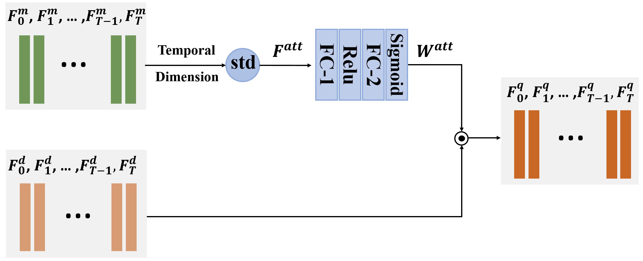
Figure 2: Illustration of the attention module for feature extraction.

III-B Feature Regularization with Gaussian Distribution

Given the frame-level quality feature $\textbf{{F}}_{\_}{i}^{q}$, the Gated Recurrent Unit (GRU) [55] layer is utilized to refine the frame-level feature by involving the temporal information. In particular, we use a fully connected layer (denoted as $FC_{\_}3$) to reduce the redundancies of VGG feature, following which the resultant feature is processed by a GRU layer,

$$\text{ $\textbf{{F}}_{\_}{i}^{gru}$ }=GRU(FC_{\_}3(\textbf{{F}}_{\_}{i}^{q})).$$ (6)

However, we argue that the $\textbf{{F}}_{\_}{i}^{gru}$ is still not generalized enough to different scenes and distortion types. To enhance the generalization capability of $\textbf{{F}}_{\_}{i}^{gru}$, we resort to feature regularization, expecting to learn the quality feature with a unified distribution. The underlying assumption of generalizing to an unseen domain is that there exists a discrete attribute separating the data into different domains. However, a naïve extension to VQA may be confused by numerous discrete or continuous attributes (e.g., scene, distortion type, motion, resolution) for domain classification. As such, instead of dividing the data into different domains, we restrict the frame-level feature subject to a mixture Gaussian distribution by a GAN based model, and moreover the mean and variance of the presumed Gaussian distribution can also be adaptively learned. To be specific, as shown in Fig. 1, we first average the extracted $\textbf{{F}}^{gru}$ of each frame as follows,

$$\textbf{{F}}^{avg}=\frac{1}{T}\sum_{\_}{i=1}^{T}\textbf{{F}}_{\_}{i}^{gru}.$$ (7)

Herein, we treat the feature $\textbf{{F}}^{avg}$ extractor as the generator $G(\cdot)$ of a GAN model and we sample the same dimension vector (denoted as $\textbf{{F}}^{gaus}$) from the prior Gaussian distribution as reference. Then the discriminator $D(\cdot)$ tries to distinguish the generated feature from the sampled vector. The GAN model is trained through the following adversarial loss,

$$\min_{\_}{G}\max_{\_}{D}E_{\_}{\mathbf{z}\sim g(\mathbf{z})}[\log D(\mathbf{z})]+E_{\_}{\mathbf{x}\sim q(\mathbf{x})}[\log(1-D(G(\mathbf{x})))],$$ (8)

where $\mathbf{z}$ is the vector $\textbf{{F}}^{gaus}$ sampled from Gaussian distribution $g(x)$, $\mathbf{x}$ is the input video and $G(\mathbf{x})$ generates the feature $\textbf{{F}}^{avg}$. When the network is trained in the first $N$ epochs, we constrain the $g(x)$ to be the standard Gaussian distribution with mean $\mu=0$ and variance $\sigma=1$. However, this imposes a strong constraint that the features in each dimension share the Gaussian distribution with identical mean and variance. Generally speaking, each dimension of the feature is expected to represent a perceptual relevance attribute for quality inference, such that they ultimately follow different Gaussian distributions parameterized by different $\mu$ and $\sigma$. This motivates us to adapt the mean and variance of prior Gaussian distribution of each dimension via learning. More specifically, to learn the parameters $\boldsymbol{\mu}=[\mu_{\_}1,\mu_{\_}2,...,\mu_{\_}L]$ and $\boldsymbol{\sigma}=[\sigma_{\_}1,\sigma_{\_}2,...,\sigma_{\_}L]$ where $L$ is the dimension of $\textbf{{F}}^{avg}$, we impose the constraint on $\textbf{{F}}^{avg}$ to regress the quality score

$$Q^{reg}=\frac{1}{L}\sum_{\_}{l=1}^{L}e^{-\frac{\left(\textbf{{F}}^{avg}(l)-\boldsymbol{\mu}(l)\right)^{2}}{\boldsymbol{\sigma}(l)^{2}}}.$$ (9)

Here, we use $Q^{reg}$ to represent the predicted quality score of the input video, and we aim to regress $Q^{reg}$ towards the ground-truth mean opinion score (MOS) via learning the optimal $\boldsymbol{\mu}$ and $\boldsymbol{\sigma}$. Moreover, $l$ indicates the $l-th$ dimension. During the training of the network, after every $N$ epochs, we use the Gaussian distribution with learned $\boldsymbol{\mu}$ and $\boldsymbol{\sigma}$ to replace the distribution in previous $N$ epochs. From the experimental results, we also find such an adaptive refreshing mechanism can further improve the performance of our model compared with standard Gaussian distribution.

III-C Pyramid Feature Aggregation

Temporal domain aggregation plays an indispensable role in objective VQA models. We consider two cognitive mechanisms in visual quality perception [56, 57]. The short-term memory effect persuades us to consider the video quality for each localized time-frame, due to the consensus that subjects are resistant in their opinion and prefer consistent quality when watching the video. Moreover, the long-term memory effect suggests that the global pooling over the whole video sequence in a coarse-to-fine manner could lead to the final video quality. Therefore, we imitate such perception mechanisms with a pyramid feature aggregation (PFA) strategy. In the PFA, the short-term memory and long-term memory are incorporated and the aggregation result is independent of the number of frames. More specifically, as illustrated in Fig. 3, in the bottom layer of the pyramid, for $\textbf{{F}}^{gru}$, we calculate its weight $\textbf{{W}}^{gru}$ by synthesizing it with its surrounding $k$ frames,

$$\textbf{{W}}^{gru}=Tahn(Conv_{\_}2(ReLu(Conv_{\_}1(\textbf{{F}}^{gru})))),$$ (10)

where the $Conv_{\_}1(\cdot)$ and $Conv_{\_}2(\cdot)$ are two 1D-CNNs and their kernel sizes are all set to $2k+1$. Moreover, $Tahn(\cdot)$ and $Relu(\cdot)$ are the activation functions, and $Tahn(\cdot)$ is defined as follows,

$$Tahn(u)=\frac{\left(e^{u}-e^{-u}\right)}{\left(e^{u}+e^{-u}\right)}.$$ (11)

Then the weighted frame-level quality feature $\textbf{{F}}^{wt}$ can be acquired,

$$\textbf{{F}}^{wt}=\textbf{{W}}^{gru}\odot\textbf{{F}}^{gru}.$$ (12)

Subsequently, the weighted frame-level features along the temporal dimension are aggregated in a pyramid manner. In general, the perceivability along the temporal dimension determines the sampling density governed by the number of layers. Herein, we empirically set the number of layers with a constant number 7. To be specific, for the $m-th$ layer ($m\in\{1,2,3...,7\}$), the weighted frame-level features are aggregated into a vector with the dimension $h\times 2^{m-1}$, where $h$ denotes the feature dimension in $\textbf{{F}}^{gru}_{\_}i$. In other words, the video is averagely divided into $2^{m-1}$ time slots, and within each time slot, average feature pooling is performed for aggregation. Finally, we concatenate the aggregated features of all layers, leading to the video-level quality feature with a constant dimension that is independent of the number of frames and frame rate, $\textbf{{F}}^{vid}\in\mathbb{R}^{h\times(2^{m}-1)}$. We first apply a fully connected layer ($FC_{\_}4$) to reduce the channel from $h$ to 1, then another fully connected layer ($FC_{\_}5$) is adopted to synthesize the pyramid aggregated features. As such, the quality of input videos can be predicted as follows,

$$\text{${Q^{vid}}$}=FC_{\_}5(FC_{\_}4(\textbf{{F}}^{vid})),$$ (13)

where ${Q^{vid}}$ is the prediction score. This strategy provides more flexibility than single layer aggregation by incorporating the variations along the temporal dimension.

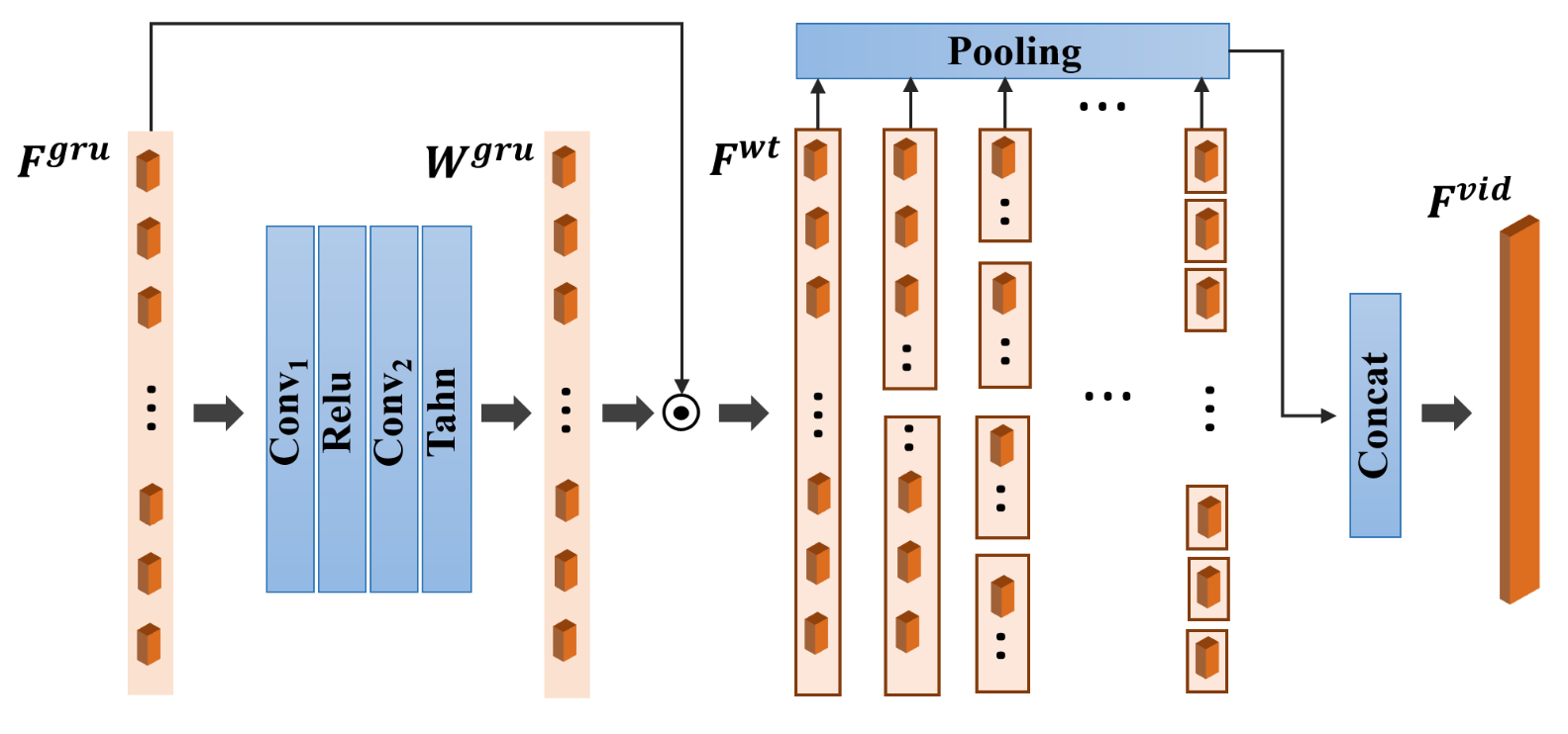
Figure 3: Illustration of PFA module.

III-D Objective Loss Function

The final loss function involves the frame-level and video-level quality regression results acquired in Eqn. (9) and Eqn. (13), as well as the distribution based feature regularization,

$$\min_{\_}{G,Q^{vid},Q^{reg}}\max_{\_}{D}\mathcal{L}^{\mathrm{vid}}+\lambda_{\_}{1}\mathcal{L}^{\mathrm{reg}}+\lambda_{\_}{2}\mathcal{R}^{\mathrm{gan}}$$ (14)

where

$$\begin{array}[]{c}\mathcal{L}^{\mathrm{vid}}=\left|Q^{vid}-MOS\right|,\\ \\ \mathcal{L}^{\mathrm{reg}}=\left|Q^{reg}-MOS\right|,\\ \\ \mathcal{R}^{\mathrm{gan}}=E_{\_}{\mathbf{z}\sim g(\mathbf{z})}[\log D(\mathbf{z})]+E_{\_}{\mathbf{x}\sim q(\mathbf{x})}[\log(1-D(G(\mathbf{x})))].\end{array}$$ (15)

Herein, $\lambda_{\_}{1}$ and $\lambda_{\_}{2}$ are two trade-off parameters. In the testing phase, we use the $Q^{vid}$ as the final quality score that our model predicts.

IV Experimental Results

IV-A Experimental Setups

IV-A1 Datasets

various video databases have been proposed for VQA, including BVI-HD [58], MCL-JCV [59], MCML-4K [60], LIVE-Netflix [61], KoNViD-1k [9], LIVE-Qualcomm [10], LIVE-VQC [11] and CVD2014 [12]. The BVI-HD VQA database is proposed for compressed video quality assessment. In MCL-JCV, a H.264/AVC encoded video dataset is constructed with a new just-noticeable difference (JND) based VQA metric. In MCML-4K dataset, the 4K ultra-high-definition (UHD) videos are compressed by three video coding techniques. LIVE-Netflix is created to simulate a typical video streaming application, using long video sequences and Netflix content. However, the above VQA databases are all constructed for compressed videos. To validate the proposed NR-VQA method on the videos in the wild, we evaluate our model on four popular VQA databases, including CVD2014 [12], LIVE-VQC [11], LIVE-Qualcomm [10] and KoNViD-1k [9].

CVD2014. In this dataset, 78 different cameras, ranging from low-quality phone cameras to dedicated digital single-lens reflex cameras, are used to capture these 234 videos. In particular, five unique scenes (traffic, city, talking head, newspaper and television) are covered with these videos of two resolutions 480P ($640\times 480$) and 720P ($1280\times 720$).

LIVE-VQC. Videos in this dataset are acquired by 80 inexperienced mobile camera users, leading to a variety of authentic distortions levels. There are in total 585 video scenes in this dataset, containing 18 different resolutions ranging from $1920\times 1080$ to $320\times 240$.

LIVE-Qualcomm. This dataset consists of 208 videos in total, which are recorded by 8 different mobile phones in 54 different scenes. Six common in-capture distortion categories are studied in this database including: noise and blockiness distortions; incorrect or insufficient color representation; over/under-exposure; autofocus related distortions; unsharpness and camera shaking. All these sequences have identical resolution 1080P and quite close frame rate.

KoNViD-1k. KoNViD-1k is the largest VQA dataset which contains in total 1200 video sequences. These videos are sampled from YFCC100m [62] dataset. Various devices are used to acquire these videos, leading to 12 different resolutions. A portion of the videos in the dataset are acquired by professional photographers, such that there is a large variance in terms of the video quality.

In Fig. 4, the sampled frames from above four datasets are shown, from which we can observe that these videos are featured by diverse scenes (e.g., indoors and outdoors), resolutions (from $1920\times 1080$ to $320\times 240$) as well as quality levels. In view of the diverse content, resolutions and frame rates in real-world applications, there has been an exponential increase in the demand for the development of VQA models with high generalization capability.

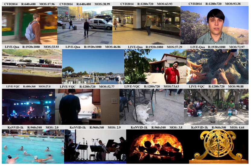
Figure 4: Sample frames from four video datasets. The corresponding resolution ($R$) and $MOS$ values are also provided.

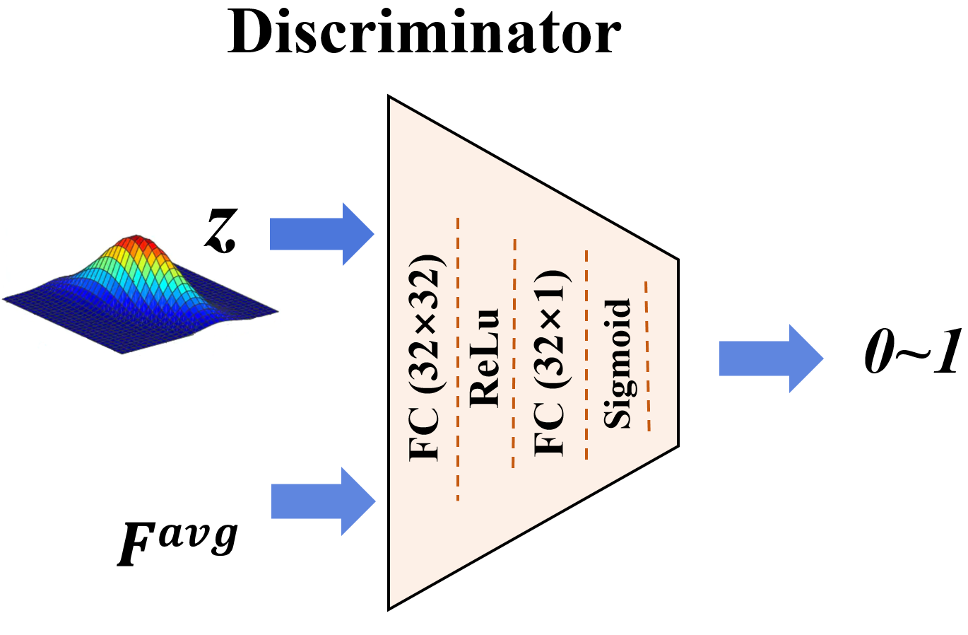
Figure 5: The architecture of the proposed discriminator.

TABLE I: Architecture of the network in the proposed method.

Layer Type		Kernel Size	Channel (in,out)	Stride
VGG16 Backbone	$CNN$×2	3	(3,64)	1
	$MaxPooling$ (stride=2)
	$CNN$×2	3	(64,128)	1
	$MaxPooling$ (stride=2)
	$CNN$×3	3	(128,256)	1
	$MaxPooling$ (stride=2)
	$CNN$×3	3	(256,512)	1
	$MaxPooling$ (stride=2)
	$CNN$×3	3	(256,512)	1
Attention module	$FC_{\_}1$		(1472,320)
	$ReLu$
	$FC_{\_}2$		(320,1472)
	$Sigmoid$
	$FC_{\_}3$		(1472,256)
	$GRU$		(256,32)
Pyramid Aggregation	$\textit{1D-}Conv_{\_}1$	15	(32,1)	1
	$ReLu$
	$\textit{1D-}Conv_{\_}2$	15	(1,1)	1
	$Tahn$
	$FC_{\_}4$		(32,1)
	$FC_{\_}5$		(127,1)

TABLE II: Performance comparisons on four datasets with cross-dataset settings. In each column, the best and second-best values are marked in boldface and underlined, respectively.

Training on KoNViD-1k		CVD2014				LIVE-Qualcomm				LIVE-VQC
		SROCC	PLCC	PWRC	KROCC	SROCC	PLCC	PWRC	KROCC	SROCC	PLCC	PWRC	KROCC
NR-IQA	NIQE	0.3856	0.4410	1.7539	0.2681	0.1807	0.1672	1.0636	0.1196	0.4573	0.4025	1.9544	0.3154
	BRISQUE	0.4626	0.5060	2.1754	0.3238	0.3061	0.3303	1.4560	0.2071	0.5805	0.5788	2.4132	0.4089
	WaDIQaM	0.6988	0.7151	3.2439	0.5081	0.4926	0.5471	1.9970	0.3545	0.6461	0.6797	3.0997	0.4634
	NIMA	0.5446	0.5836	2.4983	0.3818	0.3413	0.4011	1.5476	0.2003	0.5642	0.6204	2.5660	0.3932
	SPAQ	0.6188	0.6151	2.9039	0.4339	0.6188	0.6151	1.0560	0.4339	0.4653	0.5202	2.0865	0.3202
NR-VQA	VSFA	0.6278	0.6216	2.9590	0.4489	0.5574	0.5769	2.5571	0.3966	0.6792	0.7198	3.2374	0.4905
	TLVQM	0.3569	0.3838	1.3699	0.2442	0.4730	0.5127	2.0319	0.3290	0.5953	0.6248	2.7347	0.4268
	VIDEVAL	0.6494	0.6638	3.2831	0.4684	0.4048	0.4351	1.6906	0.2758	0.5318	0.5329	2.3962	0.3685
	CNN-TLVQM	0.6828	0.7226	3.3805	0.5003	0.6050	0.6223	3.0007	0.4354	0.7132	0.7522	3.6130	0.5218
	Ours	0.7972	0.7984	4.0625	0.5891	0.6200	0.6666	3.0198	0.4445	0.6797	0.7327	3.2126	0.4864
Training on LIVE-Qualcomm		KoNViD-1k				CVD2014				LIVE-VQC
		SROCC	PLCC	PWRC	KROCC	SROCC	PLCC	PWRC	KROCC	SROCC	PLCC	PWRC	KROCC
NR-IQA	NIQE	0.4564	0.3619	2.2080	0.3148	0.3856	0.4410	1.7539	0.2681	0.4573	0.4025	1.9544	0.3154
	BRISQUE	0.4370	0.4274	2.0893	0.2983	0.4626	0.5060	2.1754	0.3238	0.5805	0.5788	2.4132	0.4089
	WaDIQaM	0.3671	0.3510	1.7712	0.2538	0.3189	0.3255	1.1682	0.2189	0.5385	0.5377	2.2247	0.3756
	NIMA	0.2877	0.2588	1.3210	0.1948	0.2705	0.2768	1.2180	0.1842	0.3401	0.3711	1.5301	0.2306
	SPAQ	0.1330	0.1541	0.6490	0.0898	0.1663	0.1508	0.8080	0.1116	0.2854	0.3122	1.3306	01926
NR-VQA	VSFA	0.6643	0.6116	3.1701	0.4769	0.5348	0.5606	2.2852	0.3751	0.6425	0.6819	3.004	0.4613
	TLVQM	0.0347	0.0467	1.4520	0.0205	0.4893	0.4721	2.1918	0.3361	0.4091	0.3559	1.8241	0.2763
	VIDEVAL	0.1812	-0.3441	1.0368	0.1113	0.6059	0.6244	3.0739	0.4246	0.4314	0.4122	1.8863	0.2931
	CNN-TLVQM	0.0854	0.0216	0.2960	0.0692	0.2367	0.2388	0.1906	0.1924	0.0693	0.1040	0.0168	0.0567
	Ours	0.6694	0.6258	3.2347	0.4847	0.7046	0.6665	3.5204	0.5115	0.6201	0.6100	2.8957	0.4397
Training on LIVE-VQC		KoNViD-1k				CVD2014				LIVE-Qualcomm
		SROCC	PLCC	PWRC	KROCC	SROCC	PLCC	PWRC	KROCC	SROCC	PLCC	PWRC	KROCC
NR-IQA	NIQE	0.4564	0.3619	2.2080	0.3148	0.3856	0.4410	1.7539	0.2681	0.1807	0.1672	1.0636	0.1196
	BRISQUE	0.4370	0.4274	2.0893	0.2983	0.4626	0.5060	2.1754	0.3238	0.3601	0.3303	1.4560	0.2071
	WaDIQaM	0.4352	0.4451	2.0415	0.2997	0.5362	0.5417	2.5940	0.3666	0.4049	0.4207	1.1650	0.2760
	NIMA	0.5848	0.5988	2.6922	0.4105	0.3532	0.3835	1.5811	0.2427	0.3106	0.3362	1.3878	0.2098
	SPAQ	0.3542	0.3468	1.6199	0.2048	0.5494	0.4982	2.5917	0.3837	0.2714	0.3235	1.4808	0.1811
NR-VQA	VSFA	0.6584	0.6666	3.1670	0.4751	0.5061	0.5415	2.1028	0.3623	0.5094	0.5350	2.3449	0.3551
	TLVQM	0.6023	0.5943	2.8976	0.4289	0.4553	0.4749	2.0260	0.3134	0.6415	0.6534	3.1285	0.4599
	VIDEVAL	0.5007	-0.4841	2.3894	0.3422	0.5702	0.5171	2.2621	0.4125	0.3021	0.3602	1.2132	0.2064
	CNN-TLVQM	0.6431	0.6304	3.253	0.4596	0.6300	0.6568	2.9609	0.4559	0.6574	0.6696	3.2816	0.4791
	Ours	0.7085	0.7074	3.4437	0.5179	0.6894	0.6645	3.2897	0.4888	0.5952	0.6245	2.9097	0.4285
Training on CVD2014		KoNViD-1k				LIVE-Qualcomm				LIVE-VQC
		SROCC	PLCC	PWRC	KROCC	SROCC	PLCC	PWRC	KROCC	SROCC	PLCC	PWRC	KROCC
NR-IQA	NIQE	0.4564	0.3619	2.2080	0.3148	0.1807	0.1672	1.0636	0.1196	0.4573	0.4025	1.9544	0.3154
	BRISQUE	0.4370	0.4274	2.0893	0.2983	0.3061	0.3303	1.4560	0.2071	0.5805	0.5788	2.4132	0.4089
	WaDIQaM	0.4981	0.4825	2.6027	0.3456	0.2863	0.3305	1.1680	0.1906	0.4598	0.5086	1.8478	0.3222
	NIMA	0.3142	0.3013	1.5061	0.2120	0.0294	0.0628	0.1220	0.0189	0.2769	0.2933	1.3025	0.1857
	SPAQ	0.3253	0.3335	1.5053	0.2209	0.1523	0.1951	0.6067	0.0996	0.3619	0.4066	1.6269	0.2482
NR-VQA	VSFA	0.5759	0.5636	2.7670	0.4108	0.3256	0.3718	1.0461	0.2192	0.4600	0.4783	1.9002	0.3171
	TLVQM	0.5437	0.5052	2.5258	0.3758	0.3334	0.3838	1.1622	0.2279	0.5397	0.5527	2.4110	0.3803
	VIDEVAL	0.1918	-0.3260	1.2059	0.1220	0.1208	0.3315	0.5848	0.0809	0.4751	0.5167	1.7935	0.3192
	CNN-TLVQM	0.5779	0.5489	2.6767	0.4004	0.4410	0.4712	1.8800	0.2999	0.5209	0.5592	2.3276	0.3625
	Ours	0.6230	0.5764	3.0248	0.4437	0.4187	0.4965	1.8087	0.2857	0.5817	0.5751	2.6587	0.4090

IV-A2 Implementation details

we implement our model by PyTorch [63]. In Table I and Fig. 5, we detail the layer-wise network of our proposed method. In particular, we retain the original size of each frame as input without the resizing operation. The VGG-16 network is pretrained on ImageNet [64] and we fix its parameters when training. The batch size in the training phase is 128. In particular, we feed the pre-extracted deep features of the 128 videos to our model in a batch. The model is trained end-to-end with the MOS of each video as the label for regression. We adopt Adam optimizer for optimization and the learning rate is fixed to 1e-4. The weighting parameters $\lambda_{\_}{1}$, $\lambda_{\_}{2}$ in Eqn. (14) are set as 0.5 and 0.05, respectively. We train our model in an adversarial manner and the generator and discriminator are learned alternately. In particular, for each batch, we first train the discriminator by maximizing $\mathcal{R}^{\mathrm{gan}}$ loss and maintaining other parts (generator) of our model. Then we maintain the discriminator and update the generator by minimizing the $\mathcal{L}^{\mathrm{vid}}$, $\mathcal{L}^{\mathrm{reg}}$ and the discriminator loss. In both the cross-dataset and intra-dataset experiments, we fix the maximum epoch as $200$ and the model learned at the latest $200th$ epoch is used for testing. For every 20 epochs ($N=20$), we renew the mean and variance of the predefined distribution $g(x)$ in Eqn. (8). It is worth mentioning that all the experimental settings (hyper-parameters and learning strategy) are fixed. Five evaluation metrics are reported in this paper, including: Spearman’s rank-order correlation coefficient (SROCC), Kendall’s rank-order correlation coefficient (KROCC), Pearson linear correlation coefficient (PLCC), Root mean square error (RMSE) and Perceptually Weighted Rank Correlation (PWRC) [65]. In particular, the PWRC rewards the capability of correctly ranking high-quality images and suppresses the attention toward insensitive rank mistakes, which is confirmed to be more reliable in recommending the perceptually preferred IQA/VQA model. As suggested in [66], the predicted quality scores $\hat{s}$ are passed through a nonlinear logistic mapping function before computing PLCC and RMSE,

$$\tilde{s}=\beta_{\_}{1}\left(\frac{1}{2}-\frac{1}{\exp\left(\beta_{\_}{2}\left(\hat{s}-\beta_{\_}{3}\right)\right)}\right)+\beta_{\_}{4}\hat{s}+\beta_{\_}{5},$$ (16)

where $\beta_{\_}{1}$$\sim$$\beta_{\_}{5}$ are regression parameters to be fitted.

IV-B Quality Prediction Performance

In this subsection, we evaluate the performance of our method with four different cross-dataset settings to verify the generalization capability. We compare the proposed method with both NR-IQA methods including NIQE [67], BRISQ [2], WaDIQaM [30], NIMA [27], SPAQ [7] and NR-VQA methods including VSFA [35], TLVQM [33], VIDEVAL [1], and CNN-TLVQM [68].

In each setting, the models are trained on one dataset and tested on other three datasets. For deep learning based NR-IQA models, we extract two frames per second of each video in the training set and the MOS of the video is treated as the quality score of the extracted frames for model training. The results are shown in Table II, from which we can find our method can achieve the best performance on all individual cross-dataset settings which reveals the superior generalization ability of our proposed method. Compared with NR-VQA methods, we can observe that the overall performance of NR-IQA methods is not satisfactory as the temporal information is discarded. However, even the VQA based methods cannot achieve very promising performance in such challenging settings. For example, when the method VIDEV trained on LIVE-Qua dataset, the testing result of SROCC is 0.6059 on CVD2014 dataset while it is degraded significantly to 0.1812 on KoNViD-1k dataset which further demonstrates the large domain gap between the two datasets. As shown in Table II, training on CVD2014 dataset and cross-testing on other three datasets is the most challenging setting as only 234 videos and 5 scenes are involved in CVD2014. The limited data cause the over-fitting problem. However, our method still leads with a large margin over the second-best method VSFA, demonstrating the robustness and promising generalization capability of our method.

Moreover, we also provide the performance of our feature regularization module (a.k.a output of Eqn. (9)). The results comparing with the feature aggregation module are shown in Table III. From the table, we can observe that the average values (SROCC and PLCC) of the feature aggregation module outperform the feature regularization module on all cross-dataset settings, revealing higher generalization capability achieved by the feature aggregation. However, the averaged frame-wise features can also provide the global quality estimation of the input video. Therefore, we further fuse the outputs of Eqs. (9) and (13) ($Q^{reg}$ and $Q^{vid}$, respectively) with the weights set by $\lambda$ as follows:

$$Q^{{fus}}=\frac{Q^{{vid}}+\lambda Q^{{reg}}}{1+\lambda}$$ (17)

We set $\lambda$ from 0.0 - 1.8 and the experimental results are shown in Table IV. From the table, we can find the higher overall performance can be achieved when the $\lambda$ is set around 0.4. This phenomenon demonstrates that the combination of global quality information (acquired by average pooling) can finally benefit the improvement of generalization capability.

TABLE III: Performance comparisons on four datasets with cross-dataset settings. The “Frame” represents the output of feature regularization module and “Video” represents the output of feature aggregation module. The numbers in bold are the best results.

Module Selected		Tranined on CVD2014			Avg	Tranined on LIVE-Q			Avg
		LIVE-Q	LIVE-V	KoNViD-1k		CVD2014	LIVE-V	KoNViD-1k
SROCC	Frame	0.5220	0.5750	0.5063	0.5344	0.6492	0.5555	0.5763	0.5937
	Video	0.4187	0.5817	0.6230	0.5411	0.7046	0.6201	0.6694	0.6647
PLCC	Frame	0.5395	0.5780	0.4819	0.5331	0.6372	0.5897	0.5549	0.5939
	Video	0.4965	0.5751	0.5764	0.5493	0.6665	0.6100	0.6258	0.6341
Module Selected		Tranined on LIVE-V			Avg	Tranined on KoNViD-1k			Avg
		CVD2014	LIVE-Q	KoNViD-1k		CVD2014	LIVE-Q	LIVE-V
SROCC	Frame	0.6425	0.5983	0.7035	0.6481	0.7125	0.5384	0.5997	0.6169
	Video	0.6894	0.5952	0.7085	0.6644	0.7972	0.6200	0.6797	0.6990
PLCC	Frame	0.6271	0.5998	0.6912	0.6394	0.7337	0.6130	0.7112	0.6860
	Video	0.6645	0.6245	0.7074	0.6655	0.7984	0.6666	0.7327	0.7326

TABLE IV: Performance comparisons on four cross-dataset settings with different weights are set for score combination. The numbers in bold are the best results.

$\lambda$	Tranined on CVD2014			Avg	Tranined on LIVE-Q			Avg
	LIVE-Q	LIVE-V	KoNViD-1k		CVD2014	LIVE-V	KoNViD-1k
0.0	0.4187	0.5817	0.6230	0.5411	0.7046	0.6201	0.6694	0.6647
0.2	0.4342	0.5871	0.6313	0.5509	0.7010	0.6201	0.6710	0.6640
0.4	0.4491	0.5895	0.6341	0.5576	0.6958	0.6206	0.6689	0.6618
0.6	0.4605	0.5913	0.6327	0.5615	0.6928	0.6206	0.6642	0.6592
0.8	0.4723	0.5923	0.6292	0.5646	0.6887	0.6199	0.6583	0.6556
1.0	0.4781	0.5924	0.6245	0.5650	0.6868	0.6188	0.6351	0.6469
1.2	0.4847	0.5926	0.6189	0.5654	0.6858	0.6182	0.6842	0.6627
1.4	0.4906	0.5924	0.6134	0.5655	0.6845	0.6179	0.6435	0.6486
1.6	0.4963	0.5922	0.6080	0.5655	0.6833	0.6176	0.6391	0.6467
1.8	0.5016	0.5915	0.6030	0.5654	0.6820	0.6170	0.6357	0.6449
$\lambda$	Tranined on LIVE-V			Avg	Tranined on KoNViD-1k			Avg
	CVD2014	LIVE-Q	KoNViD-1k		CVD2014	LIVE-Q	LIVE-V
0.0	0.6894	0.5952	0.7085	0.6644	0.7972	0.6200	0.6797	0.6990
0.2	0.6849	0.6009	0.7123	0.6660	0.7950	0.6205	0.6830	0.6995
0.4	0.6809	0.6048	0.7145	0.6667	0.7934	0.6219	0.6843	0.6999
0.6	0.6766	0.6041	0.7158	0.6655	0.7901	0.6197	0.6850	0.6983
0.8	0.6738	0.6061	0.7166	0.6655	0.7859	0.6193	0.6842	0.6965
1.0	0.6712	0.6047	0.7167	0.6642	0.7818	0.6165	0.6837	0.6940
1.2	0.6681	0.6044	0.7168	0.6631	0.7772	0.6146	0.6834	0.6917
1.4	0.6662	0.6044	0.7168	0.6625	0.7737	0.6128	0.6821	0.6895
1.6	0.6638	0.6046	0.7166	0.6617	0.7709	0.6122	0.6806	0.6879
1.8	0.6615	0.6050	0.7162	0.6609	0.7692	0.6087	0.6787	0.6855

IV-C Quality Prediction Performance on Intra-dataset

In this subsection, to further verify the effectiveness of our method, we evaluate our method on three intra-datasets including LIVE-Qualcomm, KoNViD-1k and CVD2014. We compare the proposed method with seven existing methods including NIQE [67], BRISQ [2], CORNIA [69], VIIDEO [4], VIDEVAL [1], VSFA [35], and CNN-TLVQM [68]. More specifically, for each dataset, 80% and 20% data are used for training and testing, respectively. This procedure is repeated 10 times and the mean and standard deviation of performance values are reported in Table V. From Table V, we can observe that our method can achieve the second-best performance overall performance in terms of both the prediction monotonicity (SROCC, KROCC) and the prediction accuracy (PLCC, RMSE). In particular, for the LIVE-Qualcomm dataset and KoNVid-1k dataset, our method achieves the second-best performance which is comparable with the state-of-the-art method CNN-TLVQM, and has a large gain over other methods. This phenomenon reveals that our methods can possess the superior generalization capability without much sacrifice of performance on intra-dataset settings.

TABLE V: Performance comparisons on three VQA datasets with three intra-dataset settings. Mean and standard deviation (std) of the performance values in 10 runs are reported. The overall performance is obtained by weighted-average performance over all three databases, where weights are in proportional to the size of the dataset. In each row, the best and second-best values are marked in boldface and underlined, respectively.

Method		NIQE	BRISQUE	CORNIA	VIIDEO	VBLIINDS	VSFA	CNN-TLVQM	Ours
Overall	SROCC	0.526 (± 0.055)	0.643 (± 0.059)	0.591 (± 0.052)	0.237 (± 0.073)	0.686 (± 0.035)	0.771 (± 0.028)	0.822 (± 0.025)	0.811 (± 0.031) [t]
	KROCC	0.369 (± 0.041)	0.465 (± 0.047)	0.423 (± 0.043)	0.164 (± 0.050)	0.503 (± 0.032)	0.582 (± 0.029)	0.634 (± 0.024)	0.620 (± 0.029)
	PLCC	0.542 (± 0.054)	0.625 (± 0.053)	0.595 (± 0.051)	0.218 (± 0.070)	0.660 (± 0.037)	0.762 (± 0.031)	0.829 (± 0.021)	0.817 (± 0.032)
	RMSE	4.214 (± 0.323)	3.895 (± 0.380)	4.139 (± 0.300)	5.115 (± 0.285)	3.753 (± 0.365)	3.074 (± 0.448)	2.547 (± 0.273)	2.832 (± 0.441) [b]
LIVE-Qualcomm	SROCC	0.463 (± 0.105)	0.504 (± 0.147)	0.460 (± 0.130)	0.127 (± 0.137)	0.566 (± 0.078)	0.737 (± 0.045)	0.810 (± 0.045)	0.801 (± 0.053) [t]
	KROCC	0.328 (± 0.088)	0.365 (± 0.111)	0.324 (± 0.104)	0.082 (± 0.099)	0.405 (± 0.074)	0.552 (± 0.047)	0.629 (± 0.045)	0.620 (± 0.052)
	PLCC	0.464 (± 0.136)	0.516 (± 0.127)	0.494 (± 0.133)	-0.001 (± 0.106)	0.568 (± 0.089)	0.732 (± 0.036)	0.833 (± 0.029)	0.825 (± 0.043)
	RMSE	10.858 (± 1.013)	10.731 (± 1.33)	10.759 (± 0.939)	12.308 (± 0.881)	10.760 (± 1.231)	8.863 (± 1.042)	6.734 (± 0.815)	7.605 (± 0.935) [b]
KoNViD-1k	SROCC	0.544 (± 0.040)	0.654 (± 0.042)	0.610 (± 0.034)	0.298 (± 0.052)	0.695 (± 0.024)	0.755 (± 0.025)	0.816 (± 0.019)	0.814 (± 0.026) [t]
	KROCC	0.379 (± 0.029)	0.473 (± 0.034)	0.436 (± 0.029)	0.207 (± 0.035)	0.509 (± 0.020)	0.562 (± 0.022)	0.626 (± 0.018)	0.621 (± 0.027)
	PLCC	0.546 (± 0.038)	0.626 (± 0.041)	0.608 (± 0.032)	0.303 (± 0.049)	0.658 (± 0.025)	0.744 (± 0.029)	0.818 (± 0.019)	0.825 (± 0.043)
	RMSE	0.536 (± 0.010)	0.507 (± 0.031)	0.509 (± 0.014)	0.610 (± 0.012)	0.483 (± 0.011)	0.469 (± 0.054)	0.358 (± 0.016)	0.399 (± 0.020) [b]
CVD2014	SROCC	0.489 (± 0.091)	0.709( ± 0.067)	0.614( ± 0.075)	0.023( ± 0.122)	0.746 (± 0.056)	0.880 ( ± 0.030)	0.863 (± 0.037)	0.831 (± 0.052) [t]
	KROCC	0.358 (± 0.064)	0.518 (± 0.060)	0.441 (± 0.058)	0.021 (± 0.081)	0.562 (± 0.057)	0.705 (± 0.044)	0.677 (± 0.038)	0.657 (± 0.037)
	PLCC	0.593 (± 0.065)	0.715 (± 0.048)	0.618 (± 0.079)	-0.025 (± 0.144)	0.753 (± 0.053)	0.885 (± 0.031)	0.880 (± 0.025)	0.844 (± 0.062)
	RMSE	17.168 (± 1.318)	15.197 (± 1.325)	16.871 (± 1.200)	21.822 (± 1.152)	14.292 (± 1.413)	11.287 (± 1.943)	10.323 (± 1.134)	11.552 (± 2.014) [b]

IV-D Ablation Study

In this subsection, to reveal the functionalities of different modules in the proposed method, we perform the ablation analysis. The experiments are conducted with a cross-dataset setting (training on KoNViD-1k and testing on other three datasets). As shown in Table VI, the performance are provided in terms of SROCC and PLCC. To identify the effectiveness of the attention module used in multi-scale features extraction, we directly concatenate the mean and std pooling features without attention performed and maintain the rest of parts for training. The model is denoted as Concat in Table VI, in which we can observe that the performance on all testing sets is degraded especially on the LIVE-Qualcomm dataset. The similar phenomenon can be observed when the pyramid poling module is ablated (denoted as Ours $w/o$ PymidPooling in Table VI). The reason lies in that the videos in LIVE-Qualcomm dataset challenge both human subjects and objective VQA models, as indicated in [10]. As such, more dedicated design on both spatial and temporal domains is desired. Moreover, we remove the Gaussian distribution regularization module from the original models, leading to a model denoted as Ours $w/o$ Distribution. From the results, we can find that both the SROCC and PLCC are degraded compared with our original method (denoted as Ours) which demonstrates that the regularization on feature space is also important for the generalized VQA model.

TABLE VI: Ablation studies with the KoNViD-1k as the training data. For simplification, we denote the LIVE-Qualcomm as LIVE-Q and LIVE-VQC and LIVE-V.

Method		CVD2014	LIVE-Q	LIVE-V
Concat	SROCC	0.7466	0.5286	0.6357 [t]
	PLCC	0.7625	0.5847	0.6889 [b]
Ours $w/o$ Distribution	SROCC	0.7735	0.5900	0.6692 [t]
	PLCC	0.7638	0.6524	0.7142 [b]
Ours $w/o$ PyramidPooling	SROCC	0.7732	0.5884	0.6701 [t]
	PLCC	0.7631	0.6495	0.7173 [b]
Ours	SROCC	0.7972	0.6200	0.6797 [t]
	PLCC	0.7984	0.6666	0.7327 [b]

IV-E Visualization

To better understand the quality relevant features learned in our proposed method, we train our model on one specific dataset and visualize the quality features of all videos of the four datasets. More specifically, for each video, we first extract its feature $\textit{F}^{avg}$ (as shown in Eqn. (8)) generated with/without the Gaussian distribution based regularization, respectively. Subsequently, the feature dimension is reduced to two by T-SNE [70], as visualized in Fig. 6. We are particularly interested in the KoNViD-1k dataset due to the large number of videos with a wide-range of quality levels. As shown in Fig. 6, we can find the features of KoNViD-1k dataset and the features of other three datastes are more compact when they are regularized. More specifically, when the models are trained on the CVD2014 dataset, a larger domain gap can be observed between the KoNViD-1k dataset and the other three datasets when compared with the model trained with regularization, further verifying the effectiveness of our Gaussian distribution based regularization module.

Moreover, to verify whether the Gaussian distribution is updated from the initial standard distribution (mean $\mu=0$ and variance $\sigma=1$) of each dimension in $\textit{F}^{avg}$, we also plot the final values of mean and variance in Fig. 7 on four cross-dataset testings. We can observe that the distributions of each feature dimension is totally different from each other. For example, when the model is trained on LIVE-VQC dataset, the variance of 30-th dimension is nearly 1.4 times of the 17-th dimension, which further reveals that the quality of the video is governed by the features from different dimensions with different sensitives.

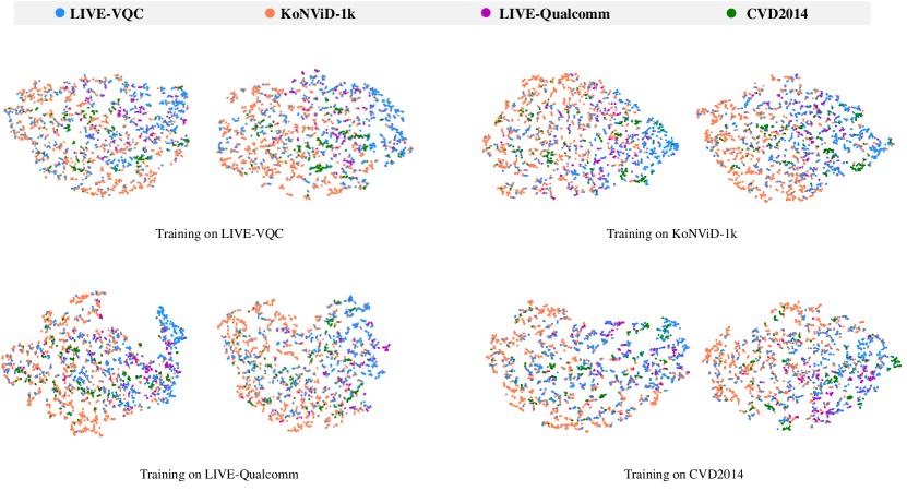
Figure 6: T-SNE visualization of the features extractions from each dataset. The dataset used for training is provided under each sub-figure.

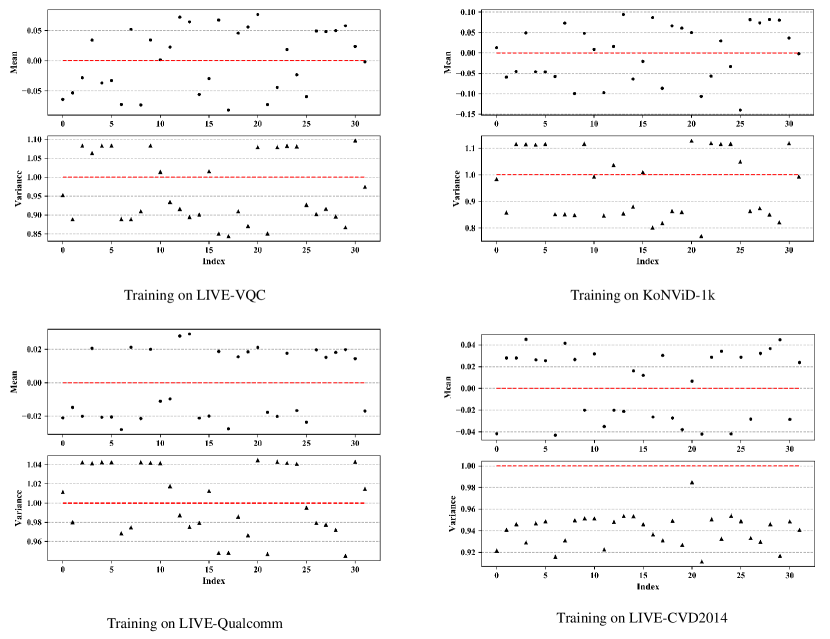
Figure 7: Mean and variance of each dimension of $\textit{F}^{avg}$ in Eqn. (8). The dataset used for training is provided under each sub-figure.

V Conclusions

In this paper, we propose an NR-VQA method, aiming for improving the generalization capability of the quality assessment model when the training and testing videos hold different content, resolutions and frame rates. The effectiveness of the proposed method, which has been validated in both cross-dataset and intra-dataset settings, arises from the feature learning based upon unified distribution constraint and pyramid temporal aggregation. The proposed model is extensible from multiple perspectives. For example, the proposed model can be further applied in the optimization tasks when the pristine reference video is not available. Moreover, the design philosophy could be further applied to other domains (e.g., high dynamic range, screen content, virtual reality).

Baoliang Chen received the B.S. degree in Electronic Information Science and Technology from Hefei University of Technology, Hefei, China, in 2015 and the M.S. degree in Intelligent Information Processing from Xidian University, Xian, China, in 2018. He was a researcher in iFlytek Inc., from 2018 to 2019. He is currently pursuing the Ph.D. degree in Department of Computer Science of City University of HongKong, HongKong. His research interests include image/video quality assessment and information security.

Lingyu Zhu received the B.S. degree from the Wuhan University of Technology in 2018 and the master’s degree from Hong Kong University of Science and Technology in 2019. He is currently pursuing the Ph.D. degree at the City University of Hong Kong. His research interests include image/video quality assessment, image/ video processing, and deep learning.

Guo Li received the B.S. degree in physics from Huazhong University of Science and Technology in 2012 and the M.S. degree in physics from Huazhong University of Science and Technology in 2016. He worked successively in Yuanfudao Company and Kingsoft Cloud Company, China. His research fields include image processing and quality assessment.

Fangbo Lu is currently working on Kingsoft Cloud Company as a Senior Algorithm Engineer, China. His research interests include video processing, video or audio codec.

Hongfei Fan received the B.S. degree in software engineering from Shanghai Jiao Tong University in 2013 and the Ph.D. degree in computer application technology from Peking University in 2017. Since July 2017, he has been working as an Algorithm Architect with Kingsoft Cloud Company, China. His research interests include video coding and image processing.

Shiqi Wang (Member, IEEE) received the B.S. degree in computer science from the Harbin Institute of Technology in 2008 and the Ph.D. degree in computer application technology from Peking University in 2014. From 2014 to 2016, he was a Post-Doctoral Fellow with the Department of Electrical and Computer Engineering, University of Waterloo, Waterloo, ON, Canada. From 2016 to 2017, he was a Research Fellow with the Rapid-Rich Object Search Laboratory, Nanyang Technological University, Singapore. He is currently an Assistant Professor with the Department of Computer Science, City University of Hong Kong. He has proposed over 50 technical proposals to ISO/MPEG, ITU-T, and AVS standards, and authored/coauthored more than 200 refereed journal articles/conference papers. He received the Best Paper Award from IEEE VCIP 2019, ICME 2019, IEEE Multimedia 2018, and PCM 2017 and is the coauthor of an article that received the Best Student Paper Award in the IEEE ICIP 2018. His research interests include video compression, image/video quality assessment, and image/video search and analysis.

References

- [1] Z. Tu, Y. Wang, N. Birkbeck, B. Adsumilli, and A. C. Bovik, “Ugc-vqa: Benchmarking blind video quality assessment for user generated content,” arXiv preprint arXiv:2005.14354, 2020.
- [2] A. Mittal, A. K. Moorthy, and A. C. Bovik, “No-reference image quality assessment in the spatial domain,” IEEE Transactions on image processing, vol. 21, no. 12, pp. 4695–4708, 2012.
- [3] L. Zhang, L. Zhang, and A. C. Bovik, “A feature-enriched completely blind image quality evaluator,” IEEE Transactions on Image Processing, vol. 24, no. 8, pp. 2579–2591, 2015.
- [4] A. Mittal, M. A. Saad, and A. C. Bovik, “A completely blind video integrity oracle,” IEEE Transactions on Image Processing, vol. 25, no. 1, pp. 289–300, 2015.
- [5] W. Liu, Z. Duanmu, and Z. Wang, “End-to-end blind quality assessment of compressed videos using deep neural networks.” in ACM Multimedia, 2018, pp. 546–554.
- [6] H. Zhu, L. Li, J. Wu, W. Dong, and G. Shi, “Metaiqa: Deep meta-learning for no-reference image quality assessment,” in Proceedings of the IEEE/CVF Conference on Computer Vision and Pattern Recognition, 2020, pp. 14 143–14 152.
- [7] Y. Fang, H. Zhu, Y. Zeng, K. Ma, and Z. Wang, “Perceptual quality assessment of smartphone photography,” in Proceedings of the IEEE/CVF Conference on Computer Vision and Pattern Recognition, 2020, pp. 3677–3686.
- [8] H. Ren, D. Chen, and Y. Wang, “Ran4iqa: restorative adversarial nets for no-reference image quality assessment,” arXiv preprint arXiv:1712.05444, 2017.
- [9] V. Hosu, F. Hahn, M. Jenadeleh, H. Lin, H. Men, T. Szirányi, S. Li, and D. Saupe, “The konstanz natural video database (konvid-1k),” in 2017 Ninth international conference on quality of multimedia experience (QoMEX). IEEE, 2017, pp. 1–6.
- [10] D. Ghadiyaram, J. Pan, A. C. Bovik, A. K. Moorthy, P. Panda, and K.-C. Yang, “In-capture mobile video distortions: A study of subjective behavior and objective algorithms,” IEEE Transactions on Circuits and Systems for Video Technology, vol. 28, no. 9, pp. 2061–2077, 2017.
- [11] Z. Sinno and A. C. Bovik, “Large-scale study of perceptual video quality,” IEEE Transactions on Image Processing, vol. 28, no. 2, pp. 612–627, 2018.
- [12] M. Nuutinen, T. Virtanen, M. Vaahteranoksa, T. Vuori, P. Oittinen, and J. Häkkinen, “Cvd2014—a database for evaluating no-reference video quality assessment algorithms,” IEEE Transactions on Image Processing, vol. 25, no. 7, pp. 3073–3086, 2016.
- [13] W. Xue, X. Mou, L. Zhang, A. C. Bovik, and X. Feng, “Blind image quality assessment using joint statistics of gradient magnitude and laplacian features,” IEEE Transactions on Image Processing, vol. 23, no. 11, pp. 4850–4862, 2014.
- [14] K. Gu, G. Zhai, X. Yang, and W. Zhang, “Using free energy principle for blind image quality assessment,” IEEE Transactions on Multimedia, vol. 17, no. 1, pp. 50–63, 2014.
- [15] A. K. Moorthy and A. C. Bovik, “Blind image quality assessment: From natural scene statistics to perceptual quality,” IEEE transactions on Image Processing, vol. 20, no. 12, pp. 3350–3364, 2011.
- [16] S. Camps, T. Houben, D. Fontanarosa, C. Edwards, M. Antico, M. Dunnhofer, E. Martens, J. Baeza, B. Vanneste, E. van Limbergen et al., “One-class gaussian process regressor for quality assessment of transperineal ultrasound images,” in Proceedings of the 1st International Conference on Medical Imaging with Deep Learning 2018. Medical Imaging with Deep Learning Conference Committee, 2018, pp. 1–10.
- [17] H. Tang, N. Joshi, and A. Kapoor, “Blind image quality assessment using semi-supervised rectifier networks,” in Proceedings of the IEEE Conference on Computer Vision and Pattern Recognition, 2014, pp. 2877–2884.
- [18] Q. Wu, H. Li, K. N. Ngan, and K. Ma, “Blind image quality assessment using local consistency aware retriever and uncertainty aware evaluator,” IEEE Transactions on Circuits and Systems for Video Technology, vol. 28, no. 9, pp. 2078–2089, 2017.
- [19] M. A. Saad, A. C. Bovik, and C. Charrier, “Blind image quality assessment: A natural scene statistics approach in the dct domain,” IEEE transactions on Image Processing, vol. 21, no. 8, pp. 3339–3352, 2012.
- [20] Y. Zhang and D. M. Chandler, “No-reference image quality assessment based on log-derivative statistics of natural scenes,” Journal of Electronic Imaging, vol. 22, no. 4, p. 043025, 2013.
- [21] Z. Chen and W. Wu, “Asymmetric foveated just-noticeable-difference model for images with visual field inhomogeneities,” IEEE Transactions on Circuits and Systems for Video Technology, vol. 30, no. 11, pp. 4064–4074, 2019.
- [22] M. Kim, K. S. Song, and M. G. Kang, “No-reference image contrast assessment based on just-noticeable-difference,” Electronic Imaging, vol. 2017, no. 12, pp. 26–29, 2017.
- [23] Z. Gu, Y. Ding, R. Deng, X. Chen, and A. S. Krylov, “Multiple just-noticeable-difference-based no-reference stereoscopic image quality assessment,” Applied optics, vol. 58, no. 2, pp. 340–352, 2019.
- [24] Q. Wu, H. Li, F. Meng, K. N. Ngan, B. Luo, C. Huang, and B. Zeng, “Blind image quality assessment based on multichannel feature fusion and label transfer,” IEEE Transactions on Circuits and Systems for Video Technology, vol. 26, no. 3, pp. 425–440, 2015.
- [25] W. Zhang, K. Ma, J. Yan, D. Deng, and Z. Wang, “Blind image quality assessment using a deep bilinear convolutional neural network,” IEEE Transactions on Circuits and Systems for Video Technology, 2018.
- [26] W. Zhang, K. Zhai, G. Zhai, and X. Yang, “Learning to blindly assess image quality in the laboratory and wild,” in 2020 IEEE International Conference on Image Processing (ICIP). IEEE, 2020, pp. 111–115.
- [27] H. Talebi and P. Milanfar, “Nima: Neural image assessment,” IEEE Transactions on Image Processing, vol. 27, no. 8, pp. 3998–4011, 2018.
- [28] N. Murray, L. Marchesotti, and F. Perronnin, “Ava: A large-scale database for aesthetic visual analysis,” in 2012 IEEE Conference on Computer Vision and Pattern Recognition. IEEE, 2012, pp. 2408–2415.
- [29] S. Su, Q. Yan, Y. Zhu, C. Zhang, X. Ge, J. Sun, and Y. Zhang, “Blindly assess image quality in the wild guided by a self-adaptive hyper network,” in Proceedings of the IEEE/CVF Conference on Computer Vision and Pattern Recognition, 2020, pp. 3667–3676.
- [30] S. Bosse, D. Maniry, K.-R. Müller, T. Wiegand, and W. Samek, “Deep neural networks for no-reference and full-reference image quality assessment,” IEEE Transactions on Image Processing, vol. 27, no. 1, pp. 206–219, 2017.
- [31] K. Manasa and S. S. Channappayya, “An optical flow-based no-reference video quality assessment algorithm,” in 2016 IEEE International Conference on Image Processing (ICIP). IEEE, 2016, pp. 2400–2404.
- [32] Y. Li, L.-M. Po, C.-H. Cheung, X. Xu, L. Feng, F. Yuan, and K.-W. Cheung, “No-reference video quality assessment with 3d shearlet transform and convolutional neural networks,” IEEE Transactions on Circuits and Systems for Video Technology, vol. 26, no. 6, pp. 1044–1057, 2015.
- [33] J. Korhonen, “Two-level approach for no-reference consumer video quality assessment,” IEEE Transactions on Image Processing, vol. 28, no. 12, pp. 5923–5938, 2019.
- [34] M. T. Vega, D. C. Mocanu, J. Famaey, S. Stavrou, and A. Liotta, “Deep learning for quality assessment in live video streaming,” IEEE signal processing letters, vol. 24, no. 6, pp. 736–740, 2017.
- [35] D. Li, T. Jiang, and M. Jiang, “Quality assessment of in-the-wild videos,” in Proceedings of the 27th ACM International Conference on Multimedia, 2019, pp. 2351–2359.
- [36] P. Chen, L. Li, L. Ma, J. Wu, and G. Shi, “Rirnet: Recurrent-in-recurrent network for video quality assessment,” in Proceedings of the 28th ACM International Conference on Multimedia, 2020, pp. 834–842.
- [37] J. You and J. Korhonen, “Deep neural networks for no-reference video quality assessment,” in 2019 IEEE International Conference on Image Processing (ICIP). IEEE, 2019, pp. 2349–2353.
- [38] K. Muandet, D. Balduzzi, and B. Schölkopf, “Domain generalization via invariant feature representation,” in International Conference on Machine Learning, 2013, pp. 10–18.
- [39] S. Erfani, M. Baktashmotlagh, M. Moshtaghi, V. Nguyen, C. Leckie, J. Bailey, and R. Kotagiri, “Robust domain generalisation by enforcing distribution invariance,” in Proceedings of the Twenty-Fifth International Joint Conference on Artificial Intelligence. AAAI Press/International Joint Conferences on Artificial Intelligence, 2016, pp. 1455–1461.
- [40] Q. Xie, Z. Dai, Y. Du, E. Hovy, and G. Neubig, “Controllable invariance through adversarial feature learning,” in Advances in Neural Information Processing Systems, 2017, pp. 585–596.
- [41] M. Ghifary, W. Bastiaan Kleijn, M. Zhang, and D. Balduzzi, “Domain generalization for object recognition with multi-task autoencoders,” in Proceedings of the IEEE international conference on computer vision, 2015, pp. 2551–2559.
- [42] Z. Xu, W. Li, L. Niu, and D. Xu, “Exploiting low-rank structure from latent domains for domain generalization,” in European Conference on Computer Vision. Springer, 2014, pp. 628–643.
- [43] S. Motiian, M. Piccirilli, D. A. Adjeroh, and G. Doretto, “Unified deep supervised domain adaptation and generalization,” in Proceedings of the IEEE International Conference on Computer Vision, 2017, pp. 5715–5725.
- [44] G. Andrew, R. Arora, J. Bilmes, and K. Livescu, “Deep canonical correlation analysis,” in International conference on machine learning. PMLR, 2013, pp. 1247–1255.
- [45] F. M. Carlucci, A. D’Innocente, S. Bucci, B. Caputo, and T. Tommasi, “Domain generalization by solving jigsaw puzzles,” in Proceedings of the IEEE Conference on Computer Vision and Pattern Recognition, 2019, pp. 2229–2238.
- [46] Y. Wang, H. Li, and A. C. Kot, “Heterogeneous domain generalization via domain mixup,” in ICASSP 2020-2020 IEEE International Conference on Acoustics, Speech and Signal Processing (ICASSP). IEEE, 2020, pp. 3622–3626.
- [47] I. J. Goodfellow, J. Shlens, and C. Szegedy, “Explaining and harnessing adversarial examples,” arXiv preprint arXiv:1412.6572, 2014.
- [48] A. Sinha, H. Namkoong, and J. Duchi, “Certifiable distributional robustness with principled adversarial training,” arXiv preprint arXiv:1710.10571, vol. 2, 2017.
- [49] H. Li, S. Jialin Pan, S. Wang, and A. C. Kot, “Domain generalization with adversarial feature learning,” in Proceedings of the IEEE Conference on Computer Vision and Pattern Recognition, 2018, pp. 5400–5409.
- [50] L. Schmidt, S. Santurkar, D. Tsipras, K. Talwar, and A. Madry, “Adversarially robust generalization requires more data,” in Advances in Neural Information Processing Systems, 2018, pp. 5014–5026.
- [51] K. Simonyan and A. Zisserman, “Very deep convolutional networks for large-scale image recognition,” arXiv preprint arXiv:1409.1556, 2014.
- [52] K. Ding, K. Ma, S. Wang, and E. P. Simoncelli, “Image quality assessment: Unifying structure and texture similarity,” arXiv preprint arXiv:2004.07728, 2020.
- [53] Y. Li, X. Ye, and Y. Li, “Image quality assessment using deep convolutional networks,” AIP Advances, vol. 7, no. 12, p. 125324, 2017.
- [54] W. Wan, J. Chen, T. Li, Y. Huang, J. Tian, C. Yu, and Y. Xue, “Information entropy based feature pooling for convolutional neural networks,” in Proceedings of the IEEE International Conference on Computer Vision, 2019, pp. 3405–3414.
- [55] K. Cho, B. Van Merriënboer, C. Gulcehre, D. Bahdanau, F. Bougares, H. Schwenk, and Y. Bengio, “Learning phrase representations using rnn encoder-decoder for statistical machine translation,” arXiv preprint arXiv:1406.1078, 2014.
- [56] S. Hochreiter and J. Schmidhuber, “Long short-term memory,” Neural computation, vol. 9, no. 8, pp. 1735–1780, 1997.
- [57] K. Zhang, W.-L. Chao, F. Sha, and K. Grauman, “Video summarization with long short-term memory,” in European conference on computer vision. Springer, 2016, pp. 766–782.
- [58] F. Zhang, F. M. Moss, R. Baddeley, and D. R. Bull, “Bvi-hd: A video quality database for hevc compressed and texture synthesized content,” IEEE Transactions on Multimedia, vol. 20, no. 10, pp. 2620–2630, 2018.
- [59] H. Wang, W. Gan, S. Hu, J. Y. Lin, L. Jin, L. Song, P. Wang, I. Katsavounidis, A. Aaron, and C.-C. J. Kuo, “Mcl-jcv: a jnd-based h. 264/avc video quality assessment dataset,” in 2016 IEEE International Conference on Image Processing (ICIP). IEEE, 2016, pp. 1509–1513.
- [60] M. Cheon and J.-S. Lee, “Subjective and objective quality assessment of compressed 4k uhd videos for immersive experience,” IEEE Transactions on Circuits and Systems for Video Technology, vol. 28, no. 7, pp. 1467–1480, 2017.
- [61] C. G. Bampis, Z. Li, A. K. Moorthy, I. Katsavounidis, A. Aaron, and A. C. Bovik, “Study of temporal effects on subjective video quality of experience,” IEEE Transactions on Image Processing, vol. 26, no. 11, pp. 5217–5231, 2017.
- [62] B. Thomee, D. A. Shamma, G. Friedland, B. Elizalde, K. Ni, D. Poland, D. Borth, and L.-J. Li, “Yfcc100m: The new data in multimedia research,” Communications of the ACM, vol. 59, no. 2, pp. 64–73, 2016.
- [63] A. Paszke, S. Gross, F. Massa, A. Lerer, J. Bradbury, G. Chanan, T. Killeen, Z. Lin, N. Gimelshein, L. Antiga et al., “Pytorch: An imperative style, high-performance deep learning library,” in Advances in neural information processing systems, 2019, pp. 8026–8037.
- [64] J. Deng, W. Dong, R. Socher, L.-J. Li, K. Li, and L. Fei-Fei, “Imagenet: A large-scale hierarchical image database,” in 2009 IEEE conference on computer vision and pattern recognition. Ieee, 2009, pp. 248–255.
- [65] Q. Wu, H. Li, F. Meng, and K. N. Ngan, “A perceptually weighted rank correlation indicator for objective image quality assessment,” IEEE Transactions on Image Processing, vol. 27, no. 5, pp. 2499–2513, 2018.
- [66] V. Q. E. Group et al., “Final report from the video quality experts group on the validation of objective models of video quality assessment,” in VQEG meeting, Ottawa, Canada, March, 2000, 2000.
- [67] A. Mittal, R. Soundararajan, and A. C. Bovik, “Making a “completely blind” image quality analyzer,” IEEE Signal processing letters, vol. 20, no. 3, pp. 209–212, 2012.
- [68] J. Korhonen, Y. Su, and J. You, “Blind natural video quality prediction via statistical temporal features and deep spatial features,” in Proceedings of the 28th ACM International Conference on Multimedia, 2020, pp. 3311–3319.
- [69] P. Ye, J. Kumar, L. Kang, and D. Doermann, “Unsupervised feature learning framework for no-reference image quality assessment,” in 2012 IEEE conference on computer vision and pattern recognition. IEEE, 2012, pp. 1098–1105.
- [70] L. v. d. Maaten and G. Hinton, “Visualizing data using t-sne,” Journal of machine learning research, vol. 9, no. Nov, pp. 2579–2605, 2008.