BiPart: A Parallel and Deterministic Multilevel Hypergraph Partitioner

Abstract.

Hypergraph partitioning is used in many problem domains including VLSI design, linear algebra, Boolean satisfiability, and data mining. Most versions of this problem are NP-complete or NP-hard, so practical hypergraph partitioners generate approximate partitioning solutions for all but the smallest inputs. One way to speed up hypergraph partitioners is to exploit parallelism. However, existing parallel hypergraph partitioners are not deterministic, which is considered unacceptable in domains like VLSI design where the same partitions must be produced every time a given hypergraph is partitioned.

In this paper, we describe BiPart, the first deterministic, parallel hypergraph partitioner. Experimental results show that BiPart outperforms state-of-the-art hypergraph partitioners in runtime and partition quality while generating partitions deterministically.

1. Introduction

A hypergraph is a generalization of a graph in which an edge can connect any number of nodes. Formally, a hypergraph is a tuple $(V,E)$ where $V$ is the set of nodes and $E$ is a set of nonempty subsets of $V$ called hyperedges. Graphs are a special case of hypergraphs in which each hyperedge connects exactly two nodes (Berge, 1973).

(a) A hypergraph

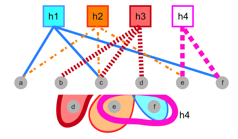
(b) Bipartite graph representation

Figure 1. Example hypergraph and the corresponding bipartite graph representation

Figure 1(a) shows a hypergraph with 6 nodes and 4 hyperedges. The hyperedges are shown as colored shapes around nodes. The degree of a hyperedge is the number of nodes it connects. In the figure, hyperedge h1 connects nodes a, c, and f, and it has a degree of three.

Hypergraphs arise in many application domains. In VLSI design, circuits are often modeled as hypergraphs; nodes in the hypergraph represent the pins of the circuit and hyperedges represent wires from the output pin of a gate to the input pins of other gates (Caldwell et al., 1999). In Boolean satisfiability, a Boolean formula can be represented as a hypergraph in which nodes represent clauses and hyperedges represent the occurrences of a given literal in these clauses. Hypergraphs are also used to model data-center networks (Qu et al., 2015), optimize storage sharding in distributed databases (Kabiljo et al., 2017), and minimize the number of transactions in data centers with distributed data (Xia et al., 2015).

1.1. Hypergraph partitioning

In many of these applications, it is necessary to partition the hypergraph into a given number of subgraphs. For example, one of the key steps in VLSI design, called placement, assigns a location on the die to each gate. Good algorithms for placement must balance competing goals: to avoid hotspots on the chip, it is important to spread out circuit components across the entire die but this may increase interconnect wire lengths, reducing the rate at which the chip can be clocked. This problem is often solved using hypergraph partitioning (Caldwell et al., 1999). Hypergraph partitioning is also used to optimize logic synthesis (Neto et al., 2019), sparse-matrix vector multiplication (Çatalyürek and Aykanat, 2011), and storage sharding (Kabiljo et al., 2017).

Formally, the k-way hypergraph partitioning problem is defined as follows. Given a hypergraph G = (V, E), the number of partitions to be created ($k\geq 2$), and an imbalance parameter ($\epsilon\geq 0$), a k-way partition $P=\{V_{1},V_{2}...,V_{k}\}$ is said to be balanced if it satisfies the constraint $|V_{i}|\leq(1+\epsilon)(|V|/k)$. Given a partition of the nodes, each hyperedge is assigned a penalty equal to one less than the number of partitions that it spans; intuitively, a hyperedge whose nodes are all in a single partition has zero penalty, and the penalty increases as the number of partitions spanned by the hyperedge increases. The penalty for the partition is defined to be the sum of the penalties of all hyperedges. Formally, $cut(G,P)=\sum_{e}(\lambda_{e}(G,P)-1)$, where $\lambda_{e}(G,P)$ is the number of partitions that hyperedge $e$ spans. The goal of hypergraph partitioning is to find a balanced partition that has a minimal cut. In some applications, hyperedges have weights, in which case the contribution to $cut(G,P)$ from each hyperedge $e$ in the definition above is multiplied by the weight of $e$.

Many partitioners produce two partitions (often called bipartitions), and this step is repeated recursively to obtain the required number of partitions.

Although graph partitioners have been studied extensively in the literature (Fiedler, 1973; Kernighan and Lin, 1970; Karypis and Kumar, 1998; Hendrickson et al., 1995), there has been relatively little work on hypergraph partitioning. In principle, graph partitioners can be used for hypergraph partitioning by converting a hypergraph into a graph, which can be accomplished by replacing each hyperedge with a clique of edges connecting the same nodes. However, this transformation increases the memory requirements of the partitioner substantially if there are many large hyperedges and may lead to poor-quality partitions (Caldwell et al., 1999). Therefore, it is often better to treat hypergraphs separately from graphs. One way to represent a hypergraph $H$ concretely is to use a bipartite graph $G$ as shown in Figure 1. In $G$, one set of nodes represents the hyperedges in $H$, the other set of nodes represents the nodes in $H$, and an edge $(u,v)$ in G is used to represent the fact that, in the hypergraph, the hyperedge represented by $u$ contains the node represented by $v$.

An ideal hypergraph partitioner has three properties.

1. The partitioner should be capable of partitioning large hypergraphs with millions of nodes and hyperedges, producing high-quality partitions within a few seconds.

2. In some domains like VLSI circuit design, the partitioner must be deterministic; i.e., for a given hypergraph, it must produce the same partitions every time it is run even if the number of threads is changed from run to run. For example, the manual post-processing in VLSI design after partitioning optimizes the placement of the cells within each partition. Many placement tools can do efficient placement only for standard cells, and if non-standard cells are used, the placement may need to be optimized manually. Deterministic partitioning is essential to avoid having to redo the placement.

3. Since hypergraph partitioners are based on heuristics, they have parameters whose optimal values may depend on the hypergraph to be partitioned. Hypergraph partitioners should permit design-space exploration of these parameters by sophisticated users.

Most variations of graph and hypergraph partitioning are either NP-complete or NP-hard (Andreev and Räcke, 2004), so heuristic methods are used in practice to find good solutions in reasonable time. Prior work in this area is surveyed in Section 2 (Karypis and Kumar, 1998; Karypis et al., 1999; Devine et al., 2006a; Çatalyürek and Aykanat, 2011; Devine et al., 2006b; Pothen et al., 1990; Heuer et al., 2019; Maleki and Burtscher, 2018).

In our experience, existing partitioners lack one or more of the desirable properties listed above. Many high-quality hypergraph partitioners like HMetis (Karypis et al., 1999), PaToH (Çatalyürek and Aykanat, 2011), and KaHyPar (Heuer et al., 2019) are serial programs. For some of the hypergraphs in our test suite, these partitioners either run out of memory or time out after an hour, as described in Section 4.

Parallel hypergraph partitioners like Zoltan (Devine et al., 2006b) and the Social Hash Partitioner from Facebook (Kabiljo et al., 2017) can handle all hypergraphs in our test suite, but they are nondeterministic (we have observed that, for a hypergraph with 9 million nodes, the edge-cut in the output of Zoltan can vary by more than 70% from run to run when using different numbers of cores). It is important to note that this nondeterminism does not arise from incorrect synchronization of parallel reads and writes but from under-specification in the program; for example, the program may make a random selection from a set, and although it is correct to choose any element of that set, different choices may produce different outputs. Parallel programming systems may exploit such don’t-care nondeterminism to improve parallel performance (Pingali et al., 2011b), but parallel partitioners with don’t-care nondeterminism will violate the second requirement listed above.

1.2. BiPart

These limitations led us to design and implement BiPart, a parallel, deterministic hypergraph partitioner that can partition all the hypergraphs in our test suite in just a few seconds. This paper makes the following contributions.

• We describe BiPart, an open-source framework for parallel, deterministic hypergraph partitioning.

• We describe application-level mechanisms that ensure that partitioning is deterministic even though the runtime exploits don’t-care nondeterminism for performance.

• We describe a novel strategy for parallelizing multiway partitioning.

• We show experimentally that BiPart outperforms existing hypergraph partitioners in either partition quality or running time, and usually outperforms them in both dimensions.

The rest of the paper is organized as follows. Section 2 describes background and related work on hypergraph partitioning. Section 3 describes BiPart, our deterministic parallel hypergraph partitioner. Section 4 presents and analyzes the experimental results on a shared-memory NUMA machine. Section 5 concludes the paper.

2. Prior Work on Graph and Hypergraph Partitioning

There is a large body of work on graph and hypergraph partitioners, so we discuss only the most closely related work in this section. It is useful to divide partitioners into geometry-based partitioners (Sec. 2.1) and topology-based partitioners (Sec. 2.2). Multilevel partitioning, discussed in Sec. 2.3, adds a different dimension to partitioning. BiPart uses a topology-based multilevel partitioning approach.

2.1. Geometry-based Partitioning

In some domains such as finite elements, the nodes of the graph are points in a metric space such as $\mathbb{R}\textsuperscript{d}$, so we can compute the distance between two nodes. The geometric notion of proximity of nodes can be used to partition the graph using techniques like k-nearest-neighbors (KNN) (Mitchell, 1997). A sophisticated geometric partitioner was introduced by Miller, Teng, and Vavasis (Miller et al., 1991). This partitioner stereographically projects nodes from $\mathbb{R}^{d}$ to a sphere in $\mathbb{R}^{d{+}1}$. The sphere is bisected by a suitable great circle, creating the partitions, and the nodes are projected back to $\mathbb{R}^{d}$ to obtain the partitions.

When there is no geometry associated with the nodes of a graph, embedding techniques can be used to map nodes to points in $\mathbb{R}^{d}$ in ways that try to preserve proximity of nodes in the graph; geometry-based partitioners can then be used to partition the embedded graph.

One powerful but expensive embedding technique is based on computing the Fiedler vector of the Laplacian matrix of a graph (Fiedler, 1973). The Fiedler vector is the eigenvector corresponding to the second smallest eigenvalue of the Laplacian matrix. The Fiedler vector is a real vector (it can be considered an embedding of the nodes in $\mathbb{R}^{1}$) and the signs of its entries can be used to determine how to partition the graph. Several spectral partitioners based on this idea were implemented and studied in the mid-90’s (Pothen et al., 1990). They can produce good graph partitions since they take a global view of the graph, but they are not practical for large graphs.

Heuristic embedding techniques known as node2vec or DeepWalk are currently receiving a lot of attention in the machine-learning community (Grover and Leskovec, 2016; Perozzi et al., 2014). These techniques are based on random walks in the graph to estimate proximity among nodes, and these estimates are used to compute the embedding. Techniques like stochastic gradient descent (SGD) are employed to iteratively improve the embedding.

Unfortunately, all embedding techniques we know of are computationally intensive so they cannot be used for large graphs without geometry if partitioning is to be done quickly.

2.2. Topology-based Partitioning

In contrast to geometry-based partitioners, topology-based partitioners work only with the connectivity of nodes in the graph or hypergraph. These partitioners generally start with some heuristically chosen partitioning and then apply local refinements to improve the balance or the edge cut until a termination condition is reached.

Kernighan and Lin invented one of the first practical graph partitioners. An initial bipartition of the graph is obtained using a technique such as a breadth-first traversal of the graph, starting from an arbitrary node and terminating when half the nodes have been touched. Given such a partitioning of the graph that is well balanced, the algorithm (usually called the KL algorithm) attempts to reduce the cut by swapping pairs of nodes between the partitions until a termination criterion is met (Kernighan and Lin, 1970).

Fiduccia and Mattheyses generalized this algorithm to hypergraphs (their algorithm is usually referred to as the FM algorithm) (Fiduccia and Mattheyses, 1982). It starts by computing the gain values for each node, where gain refers to the change in the edge cut if a node were moved to the other partition. The algorithm executes in rounds; in each round, a subset of nodes are moved from their current partition to the other partition. A greedy algorithm is used to identify this subset: the node with the highest gain value is selected to be moved, the gain values of its neighbors are updated accordingly, and the process is repeated with the remaining unmoved nodes until all nodes are moved exactly once. At the end of every round, the algorithm picks the maximal prefix of these moves that results in the highest gain and moves the rest of the nodes back to their original partition. The overall algorithm terminates when no gain is achieved in the current round.

Experimental studies show that the quality of the partitions produced by these techniques depends critically on the quality of the initial partition. Intuitively, these algorithms perform local optimization, so they can improve the quality of a good initial partition but they cannot find a high quality partition if the initial partition is poor, since this requires global optimization.

2.3. Multilevel Graph Partitioning

Multilevel partitioning techniques attempt to circumvent the limitations of the algorithms described above rather than replace them with an entirely new algorithm. This approach was first explored for graphs (Bui and Jones, 1993; Barnard and Simon, 1993; Karypis and Kumar, 1998) and later extended to hypergraphs in the HMetis partitioner (Karypis et al., 1999). Since every graph is a hypergraph, we use the term hypergraph to include graphs in the rest of the paper.

Multilevel hypergraph partitioning consists of three phases: coarsening, initial partitioning, and refinement.

• Coarsening: For a given hypergraph $G_{f}$, a coarsened hypergraph $G_{c}$ is created by merging pairs of nodes in $G_{f}$. We call $G_{c}$ the coarsened hypergraph and $G_{f}$ the fine-grained hypergraph. This process can be applied recursively to the coarsened hypergraph, creating a chain of hypergraphs in which the first hypergraph is the initial hypergraph and the final hypergraph is a coarsened hypergraph that meets some termination criterion (e.g., its size is below some threshold).

• Initial partitioning: The coarsest hypergraph is partitioned using any of the techniques discussed in Sections 2.1 and 2.2.

• Refinement: For each pair $G_{c}$ and $G_{f}$, the partitioning of $G_{c}$ is projected onto $G_{f}$ and then refined, starting from the most coarsened hypergraph and finishing with the input hypergraph.

Various heuristics have been implemented for these three phases. For example, heavy-edge matching, where a node tries to merge with the neighbor with which it shares the heaviest weighted edge, is widely used in coarsening (Karypis and Kumar, 1998). Techniques frequently used in refinement include swapping pairs of nodes from different partitions, as in the KL algorithm, or moving nodes from one partition to another, as in the FM algorithm. Most of these heuristics were designed for sequential implementations so they cannot be used directly in a parallel implementation.

2.4. Parallel Hypergraph Partitioning

Hypergraph partitioners should be parallelized to prevent them from becoming the performance bottleneck in hypergraph processing. Zoltan (Devine et al., 2006b) and Parkway (Trifunović and Knottenbelt, 2008) are parallel hypergraph partitioners based on the multilevel scheme. HyperSwap (Yang et al., 2016) is a distributed algorithm that partitions hyperedges instead of nodes. The Social Hash partitioner (Kabiljo et al., 2017) is another distributed partitioner for balanced k-way hypergraph partitioning.

One disadvantage of these parallel hypergraph partitioners is that their output is nondeterministic. For example, in the coarsening phase, it may be desirable to merge a given node $V_{1}$ with either node $V_{2}$ or node $V_{3}$. In a parallel implementation, slight variations in the internal timing between executions may result in choosing different nodes for merging, producing different partitions of the same input graph. However, many applications require deterministic partitioning, as discussed in Section 1.

2.5. Ensuring determinism

The problem of ensuring deterministic execution of parallel programs with don’t-care nondeterminism has been studied at many abstraction levels. At the systems level, there has been a lot of work on ensuring that parallel threads communicate in a deterministic manner (Devietti et al., 2011; Hower et al., 2011; Kaler et al., 2016). For many programs, this ensures deterministic output if the program is executed on the same number of threads in every run. However, it does not address our requirement that the output of the partitioner must be the same even if the number of threads on which it executes is different in different runs. Moreover, these solutions usually result in a substantial slowdown (Nguyen et al., 2014; Devietti et al., 2011).

For nested task-parallel programs, an approach called internal determinism has been proposed to ensure that the program is executed in deterministic steps, thereby ensuring that the output is deterministic as well (Blelloch et al., 2012). The Galois system solves the determinism problem in its task scheduler (Nguyen et al., 2014), which finds independent sets of tasks in an implicitly constructed interference graph. To guarantee a deterministic schedule, the independent set must be selected in a deterministic fashion. This is achieved without building an explicit interference graph. The neighborhood items of a task are marked with the task ID, and ownership of neighborhood items with lower ID values are stolen during the marking process. An independent set is then constructed by selecting the tasks whose neighborhood locations are all marked with their own ID values.

Both these solutions guarantee that the output does not depend on the number of threads used to execute the program. However, our experiments showed that these generic, application-agnostic solutions are too heavyweight for use in hypergraph partitioning, so we devised a lightweight application-specific technique for ensuring determinism with substantially less overhead as described in Section 3.

3. BiPart: A Deterministic Parallel Hypergraph Partitioner

This sections describes BiPart, our deterministic parallel multilevel hypergraph partitioner. BiPart produces a bipartition of the hypergraph, and it is used recursively on these partitions to produce the desired number of partitions.

3.1. Coarsening

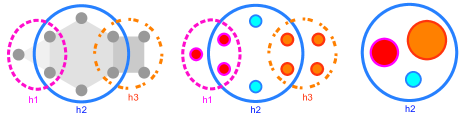
Figure 2. Multi-node coarsening: (a) a hypergraph with 3 hyperedges, h1, h2, and h3 (left). (b) multi-node matching matches nodes within a hypergraph (center). (c) merging matched nodes coarsen hypergraph (right).

Algorithm 1 Parallel Matching Policy

1:Input: $fineGraph$, $policy$;

2:/* Initialize node priorities */

3:for all nodes $node\in fineGraph$ in parallel do

4:    $node.priority\leftarrow\infty$

5:    $node.rand\leftarrow\infty$

6:    $node.hedgeid\leftarrow\infty$

7:/* Assign priorities based on the policy (e.g. low degree hyperedges) */

8:for all hyperedges $hedge\in fineGraph$ in parallel  do

9:    $hedge.priority\leftarrow degree(hedge)$

10:    $hedge.rand\leftarrow hash(hedge.id)$

11:    for $node\in hedge$ do

12:         $node.priority\leftarrow atomicMin(node.priority,$

13:                              $hedge.priority)$     

14:/* Assign a second priority (hash of hedge id) */

15:for all hyperedges $hedge\in fineGraph$ in parallel  do

16:    for node $\in$ hedge do

17:         if $hedge.priority==node.priority$ then

18:             $node.rand\leftarrow atomicMin(node.rand,hedge.rand)$              

19:/* Assign each node to its incident hyperedge with highest priority */

20:for all hyperedges $hedge\in fineGraph$ in parallel  do

21:    for node $\in$ hedge do

22:         if $hedge.rand==node.rand$ then

23:             $node.hedgeid\leftarrow atomicMin(node.hedgeid,$

24:                                   $hedge.id)$              

Algorithm 2 Parallel Coarsening

1:Input: $fineGraph$, $policy$; Output: $coarseGraph$

2:Find a multi-node matching $M$ of $fineGraph$ using Algorithm 1

3:/* Merge nodes of the finer graph */

4:for all hyperedges $hedge\in fineGraph$ in parallel do

5:    $S$: Set of nodes in $hedge$ that are matched

6:    if $|S|>1$ then

7:         $N\leftarrow$ Merge nodes in $S$

8:         for all $node\in S$ do

9:             $parent(node)\leftarrow N$               

10:/* Merge singleton nodes with an already merged node */

11:for all hyperedges $hedge\in fineGraph$ in parallel  do

12:    $S$: Set of nodes in $hedge$ that are matched

13:    if $|S|=1$ and there exist an already merged node $v\in hedge$  then

14:         $v$: Merged nodes in hedge with smallest weight

15:         Merge node $u$ in $S$ with $v$

16:         $parent(u)\leftarrow parent(v)$

17:/* Self merge singleton nodes */

18:    else if $|S|=1$ then

19:         $parent(S)\leftarrow S$     

20:/* Create hyperedges in the coarsened graph */

21:for all hyperedges $hedge\in fineGraph$ in parallel  do

22:    $parents\leftarrow\emptyset$

23:    for all $node\in hedge$ do

24:         if $parent(node)\notin parents$ then

25:             $N\leftarrow coarseGraph.createNode(parent(node))$

26:             $parents.add(parent(node))$              

27:    if $|parents|>1$ then

28:         $E\leftarrow coarseGraph.createHyperedge()$

29:         $parent(hedge)\leftarrow E$

30:         for all $node\in parents$ do

31:             $includeNodeInEdge(E,node)$              

The goal of coarsening is to create a series of smaller hypergraphs until a small enough hypergraph is obtained that can be partitioned using a simple heuristic. Intuitively, coarsening finds nodes that should be assigned to the same partition and merges them to obtain a smaller hypergraph. However, it is important to reduce the size of hyperedges as well since this enables the subsequent refinement phase to be more effective (FM and related algorithms are most effective with small hyperedges).

Coarsening can be described using the idea of matchings from graph theory (Berge, 1973).

Hyperedge matching::

A hyperedge matching of a hypergraph $H$ is an independent set of hyperedges such that no two of them have a node in common. In Figure 1, {h3, h4} is a hyperedge matching.

Node matching::

A node matching of a hypergraph $H$ is a set of node pairs $(u,v)$, where $u$ and $v$ belong to the same hyperedge such that no two pairs have a node in common. In Figure 1, {(a,e), (b,c)} is a node matching.

Multi-node matching::

BiPart uses a modified version of node matching called multi-node matching, where instead of node pairs we have a partition of the nodes of $H$ such that each node set in the partition contains nodes belonging to one hyperedge. In Figure 1, {(a,e), (b,c,d), (f)} is a multi-node matching.

Coarsening can be performed by contracting nodes or hyperedges. In the node coarsening scheme, a node matching is first computed and the nodes in each node pair in the matching are then merged together. Hyperedge coarsening computes a hyperedge matching, and all nodes connected by a hyperedge in this matching are merged to form a single node in the coarsened hypergraph.

In contrast, BiPart uses multi-node matching, which has advantages over both node coarsening and hyperedge coarsening. A hyperedge disappears from a coarsened graph only after all its member nodes are merged into one node. In node coarsening, the number of hyperedges may stay roughly the same even after merging the nodes in the matching. Similarly in hyperedge coarsening, the hyperedge matching may have a very small size and may result in only a small reduction in the size of the hypergraph. The coarsening phase in BiPart consists of two parts: finding a multi-node matching and the coarsening algorithm.

Table 1. Matching policies for multi-node matching

Policy	Policy Description
LDH	Hyperedges with lower degree have higher priority
HDH	Hyperedges with higher degree have higher priority
LWD	Lower weight hyperedges have higher priority
HWD	Higher weight hyperedges have higher priority
RAND	Priority assigned by a deterministic hash of ID value

3.1.1. Finding a multi-node matching

Algorithm 2 lists the pseudocode of multi-node matching. BiPart computes a multi-node matching in the following way: First, every hyperedge is assigned a priority based on a matching policy and a deterministic hash of its ID value (Lines 9 - 10). The matching policy can be based on the degree of the hyperedge, weight, etc. Table  1 lists the available matching policies for BiPart. Every node is then assigned a piority value, which is the minimum across all its incident hyperedges (Lines 11-13). In case many hyperedges have identical degrees, every node is assigned a second priority value (Lines 15-18) to reduce contention. Finally, every node matches itself to one of its incident hyperedges with the highest priority, e.g., the hyperedge with the lowest degree and with the lowest hashed value (in case the hyperedges have the same degree) (Lines 20- 24). The nodes that are matched to the same hyperedge are then grouped together, resulting in a deterministic multi-node matching.

3.1.2. Coarsening Algorithm

Algorithm 2 lists the pseudocode of a single phase of the coarsening algorithm used in BiPart. We perform this step repeatedly for at most coarseTo iterations. Coarsening consists of two steps. First, BiPart merges all the nodes that are matched to the same hyperedge into a single node in the coarsened graph (Lines 2-9). For optimization purposes, we ignore the singleton sets and BiPart instead merges nodes in such sets with a neighbor node that has been merged in the previous step (Lines 13-19).

Figure 2 illustrates this on a hypergraph with nine nodes and three hyperedges h1, h2, and h3. In the first step, BiPart performs multi-node matching (priority is with the low degree hyperedges (LDH)), Figure 2 (center). Figure 2 (right) shows the result of this matching. The nodes in each of the disjoint sets in the matching are merged into a single node. Note that, since all nodes of hyperedges h1 and h3 are merged to a single node, we can remove those hyperedges and only h2 remains in the hypergraph.

3.1.3. Ensuring Determinism.

Step 2 in the coarsening phase, which finds a multi-node matching of the hypergraph, is a potential source of nondeterminism. The approach presented in Section 3.1.1 yields a deterministic multi-node matching. This matching is used to coarsen the graph deterministically.

3.2. Initial Partitioning

Algorithm 3 Initial Partitioning Algorithm

1:Input: coarsest graph $G_{x}=(V_{x},E_{x})$

2:Output: Partitions $P_{0}$ and $P_{1}$.

3:$P_{0}$ = {}; $P_{1}$ = $V_{x}$

4:n = $|V_{x}|$

5:Compute move gain values for nodes in $P_{1}$ using Algorithm 4

6:while $|P_{0}|<|P_{1}|$ do

7:    Pick $\sqrt{n}$ nodes from $P_{1}$ with highest gain values (break ties using node ID) and move them to $P_{0}$ in parallel

8:    Re-compute move gain values for nodes in $P_{1}$ using Algorithm 4

The goal of this step is to obtain a good bipartition of the coarsest graph. There are many ways to accomplish this but the key idea in most algorithms is to maintain two sets of nodes $P_{0}$ and $P_{1}$ where $P_{0}$ and $P_{1}$ contain the nodes assigned to partitions $0$ and $1$, respectively. Iteratively, some nodes from $P_{1}$ are selected and moved to $P_{0}$ (assuming $P_{0}$ is smaller than $P_{1}$) until the balance condition is met.

The selection of nodes can be implemented in many ways. A simple approach is to do a breadth-first search (BFS) of the graph starting from some arbitrary vertex. In this approach, nodes on the BFS frontier are selected at each step for inclusion in the partition. The greedy graph-growing partitioning algorithm (GGGP) used in Metis maintains gain values for every node $v$ in $P_{1}$ (i.e., the decrease in the edge cut if $v$ is moved to the growing partition) and it always picks the node with the highest gain at each step and updates the gain values of the remaining nodes in $P_{1}$. However, this GGGP approach is inherently serial.

Instead, BiPart uses a more parallel approach to obtain an initial partition. The approach used in BiPart is the following. Like GGGP, we maintain gain values for nodes in $P_{1}$, but we pick the top $\sqrt{n}$ nodes with the highest gain values in each step and move them to $P_{0}$ (here $n$ denotes the number of nodes in the coarsest graph). We then re-compute the gain values of all nodes in $P_{1}$. This gives us a good parallel algorithm for computing the initial partition. Algorithm 3 lists the pseudocode.

Algorithm 4 describes the pseudocode for computing move gain values. It is based on the approach used in the FM algorithm (Fiduccia and Mattheyses, 1982).

Algorithm 4 Compute Move-Gain Values

Input: Graph $G=(V,E)$, $P_{0}$ and $P_{1}$ are the two partitions

1:Initialize $Gain(u)$ to $0$ for all $u\in V$ in parallel

2:for all hyperedges $hedge\in E$ in parallel do

3:    $n_{0}$ $\leftarrow$ number of nodes in $P_{0}\cap hedge$

4:    $n_{1}\leftarrow$ number of nodes in $P_{1}\cap hedge$

5:    for $u\in hedge$ do

6:         $i\leftarrow$ partition of $u$

7:         if $n_{i}==1$ then $\triangleright$ $u$ is the only node from $P_{i}$ in $hedge$

8:             $Gain(u)\leftarrow Gain(u)+1$

9:         else if $n_{i}==|hedge|$ then $\triangleright$ all nodes are in $P_{i}$

10:             $Gain(u)\leftarrow Gain(u)-1$              

3.2.1. Ensuring Determinism.

In the initial partitioning phase, nondeterminism may be present in Line 5 of Algorithm  3 where we need to pick a node $v$ with highest gain value and there are multiple nodes with the same highest gain. To ensure determinism, BiPart again breaks ties using node IDs.

3.3. Refinement Phase

The third phase of the overall partitioning algorithm is the refinement phase. The goal of this phase is to improve on the bipartition obtained from the initial partitioning. This phase runs a refinement algorithm on the sequence of graphs obtained during the coarsening phase, starting from the coarsest graph and terminating at the original input graph. The FM refinement algorithm described in Section 2.2 is inherently serial and cannot be used for large graphs as it is, since it needs to make individual moves for every node in every pass. Our refinement algorithm, in contrast, makes parallel node moves, thus speeding up the process. However, this approach may result in a poor edge cut since it does not choose the best prefix of moves, unlike the FM algorithm. We address this issue by ensuring that we only move nodes with high or positive gain values.

Another major difference in our refinement algorithm is that we do not consider the weight of the nodes when making these moves. This helps in speeding up the algorithm but may result in an unbalanced partition. We resolve this possible issue by running a separate balancing algorithm after the refinement. Algorithm 5 provides the pseudocode of our refinement approach. The input to the algorithm is an integer iter that specifies the number of rounds of refinement to be performed; a larger number of rounds may improve partition quality at the cost of extra running time.

Algorithm 5 Refinement Algorithm

1:Input: $iter$: refinement iterations; Partitions $P_{0}$ and $P_{1}$

2:Initialization: Project bipartition from coarsened graph

3:for $iter$ iterations do

4:       Compute move gain values for all nodes using Algo 4

5:       $L_{0}\leftarrow$ nodes in $P_{0}$ with gain value $\geq 0$

6:       $L_{1}\leftarrow$ nodes in $P_{1}$ with gain value $\geq 0$

7:       Sort nodes in $L_{0}$ and $L_{1}$ with gain value as the key (break ties using node IDs)

8:       $l_{min}\leftarrow\min{(|L_{0}|,|L_{1}|)}$

9:       Swap $l_{min}$ nodes with highest gain values between partitions $P_{0}$ and $P_{1}$ in parallel

10:Check if the balance criterion is satisfied. Otherwise, move highest gain nodes from the higher weighted partition to the other partition, using a variant of Algorithm 3.

3.3.1. Ensuring Determinism.

In the refinement phase, the only step with potential nondeterminism is Line 7, in which we create a sorted ordering of the nodes based on their gain values, since there can be multiple nodes with the same gain. BiPart breaks ties between such nodes using their IDs.

3.4. Tuning parameters

Multilevel hypergraph partitioning algorithms like BiPart have a number of tuning parameters whose values can affect the quality and runtime of the partitioning. For BiPart, the three most important tuning parameters are the following.

The first tuning parameter controls the maximum number of levels of coarsening to be performed before the initial partitioning. Most hypergraph partitioners coarsen the hypergraph until the coarsest hypergraph is very small (e.g., PaToH (Çatalyürek and Aykanat, 2011) terminates its coarsening phase when the size of the coarsened hypergraph falls below 100). Although one would expect more coarsening steps to produce a better partitioning, this is not always the case. For some hypergraphs, we end up with heavily weighted nodes (the weight is the number of merged nodes represented by that node) and processing such nodes in the refinement phase is expensive since they can cause balance problems. In Section 4, we study the performance impact of terminating the coarsening phase at different levels. The default value used in BiPart is 25.

The second tuning parameter controls the iteration count in the refinement phase. To obtain the best solution, we can run the refinement until convergence (i.e., until the edge cut does not change anymore). However, this strategy is very slow and thus infeasible for large hypergraphs, which are the focus of this work. BiPart, by default, uses only 2 refinement iterations.

The final tuning parameter is selecting a matching policy for finding a multi-node matching in a hypergraph. Table 1 shows the different matching policies available in BiPart. Some of these policies are based on hyperedge degrees or on the weight of the hyperedge. More policies can be added to the framework by the user. The best choice for the policy depends on the structure of the graph, and different policies can result in different partitioning quality as well as different convergence rates. For the experimental results in Section 4, we used LDH, HDH, or RAND, depending on the input hypergraph.

BiPart exposes these tuning parameters to the application developer but also provides default values for use by novices. Section 4 studies the effect of changing these parameters.

3.5. Parallel Strategy for Multiway Partitioning

Multiway partitioning for obtaining $k$ partitions can be performed in two ways: direct partitioning and recursive bisection. In direct partitioning, the hypergraph obtained after coarsening is divided into $k$ partitions and these partitions are refined during the refinement phase. Recursive bisection uses a divide-and-conquer approach by recursively creating bipartitions until the desired number of partitions is obtained.

In this paper, we present a novel nested $k$-way approach for obtaining $k$ partitions. At each level of the divide-and-conquer tree, we apply the three phases of multilevel partitioning to all the subgraphs at that level. Intuitively, the divide-and-conquer tree is processed level-by-level, and each phase of the multilevel partitioning algorithm is applied to all the subgraphs at the current level. Algorithm 6 presents the pseudocode of our nested $k$-way approach.

Algorithm 6 Nested $k$-Way Algorithm

1:Input: $k$

2:for $level$ $l=1$ to $\lceil\log k\rceil$ iterations do

3:       Construct subgraphs $G_{1},G_{2},\ldots,G_{i}$ (where $i=2^{l-1}$) such that $G_{j}$ contains nodes that are in partition $j$

4:       $Coarsen$ $(G_{1},G_{2},\ldots,G_{i})$

5:       $Partition$ $(G_{1},G_{2},\ldots,G_{i})$

6:       $Refine$ $(G_{1},G_{2},\ldots,G_{i})$

This algorithm allows us to run the parallel loops over the entire edge list of the original hypergraph instead of running them over edge lists for each subgraph separately, which yields a significant reduction of the overall running time. In Section 4.4, we present experimental results for obtaining $k$ partitions using this approach.

4. Experiments

We implement BiPart in the Galois 6.0 system, compiled with g++ 8.1 and boost 1.67 (library, [n.d.]). Galois is a library of data structures and a runtime system that exploits parallelism in irregular graph algorithms expressed in C++ (Pingali et al., 2011a; Nguyen et al., 2013).

Table 2 describes the 11 hypergraphs that we use in our experiments. The hypergraphs WB, NLPK, Webbase, Sat14, and RM07R are from the SuiteSparse Matrix Collection (Davis and Hu, 2011), Xyce and Circuit1 are netlists from Sandia Laboratories (Devine et al., 2006b), Leon is a hypergraph derived from a netlist from the University of Utah, and IBM18 is from the ISPD 98 VLSI Circuit Benchmark Suite. Random-10M and Random-15M are two hypergraphs that we synthetically generated for the experiments.

All experiments are done on a machine running CentOS 7 with 4 sockets of 14-core Intel Xeon Gold 5120 CPUs at 2.2 GHz, and 187 GB of RAM in which there are 65,536 huge pages, each of which has a size of 2 MB.

We benchmarked BiPart against three third-party partitioners: (i) Zoltan 3.83 (Zoltan is designed to work in a distributed environment; for our experiments, we run Zoltan with MPI in a multi-threaded configuration), (ii) KaHyPar (direct k-way partitioning setting), the state-of-the-art partitioner for high-quality partitioning, and (iii) HYPE, a recent serial, single-level bipartitioner (Mayer et al., 2018). Zoltan and KaHyPar were described in Section 2.

The balance ratio for these experiments is 55:45. Since Zoltan is nondeterministic, the runtime and quality we report is the average of three runs. BiPart numbers are obtained using the configuration discussed in Section 3.

Table 2. Benchmark Characteristics

	Hypergraph		Bipartite
			Representation
Name	Nodes	Hyperedges	Edges
Random-15M	$15,000,000$	$17,000,000$	$280,605,072$
Random-10M	$10,000,000$	$10,000,000$	$115,022,203$
WB	$9,845,725$	$6,920,306$	$57,156,537$
NLPK	$3,542,400$	$3,542,400$	$96,845,792$
Xyce	$1,945,099$	$1,945,099$	$9,455,545$
Circuit1	$1,886,296$	$1,886,296$	$8,875,968$
Webbase	$1,000,005$	$1,000,005$	$3,105,536$
Leon	$1,088,535$	$800,848$	$3,105,536$
Sat14	$13,378,010$	$521,147$	$39,203,144$
RM07R	$381,689$	$381,689$	$37,464,962$
IBM18	$210,613$	$201,920$	$819,697$

4.1. Comparison with Other Partitioners

Table 3 compares BiPart results with those obtained by running Zoltan, KaHyPar and HYPE. BiPart is executed on 14 threads, and Zoltan is executed on 14 processes, while KaHyPar, and HYPE are executed on a single thread since they are serial codes.

KaHyPar produces high-quality partitions but it took more than 1800 seconds to partition large graphs such as Random-10M, Random-15M, webbase, and Sat14. For the hypergraphs that KaHyPar can partition successfully, BiPart is always faster but worse in quality. HYPE runs on all inputs but the execution time and the quality of the partitions are always worse than BiPart.

Zoltan was able to partition all the hypergraphs in our test suite except for the largest hypergraph, Random-15M. For the three largest hypergraphs Random-10M, NLPK and WB, BiPart is roughly 4X faster than Zoltan while producing partitions of comparable quality. We also compared our results with other hypergraph partitioners, such as PaToH (Çatalyürek and Aykanat, 2011) and HMetis (Karypis et al., 1999). We observed that the parallel execution time of BiPart is better than HMetis’s and PaToH’s serial time on large inputs. Since the source code for these partitioners is not available and due to the space constraints, we do not list those results here. We did not compare our results with Parkway since it frequently produces segfaults.

Table 3. Performance of hypergraph partitioners (time is measured in seconds)

	BiPart (14)		Zoltan (14)		HYPE (1)		KaHyPar (1)
Inputs	Time	Edge cut	Time	Edge cut	Time	Edge cut	Time	Edge cut
Random-15M	85.4	13,968,401	$-$	$-$	$>1,800$	$15,628,206$	¿ 1,800	$-$
Random-10M	35.2	7,588,493	133.6	8,206,642	$>1,800$	$8,816,800$	¿ 1,800	$-$
WB	7.9	13,853	31.4	35,212	42.2	819,661	581.5	11,457
NLPK	5.8	98,010	27.6	76,987	58.8	651,396	784.3	59,205
Xyce	1.3	1,134	4.1	1,190	11.8	549,364	412.4	420
Circuit1	0.7	3,439	4.2	2,314	10.9	371,700	524.1	2,171
Webbase	0.3	624	1.2	1,645	2.4	455,492	¿ 1,800	$-$
Leon	0.9	112	5.4	81	3.8	32460	354.6	59
Sat14	7.6	15,394	44.3	5,748	61.3	524317	¿ 1,800	$-$
RM07R	0.8	22,350	3.9	56,296	19.1	151,570	880.0	17,532
IBM18	0.2	2,669	0.4	2,462	1.0	52,779	453.9	1,915

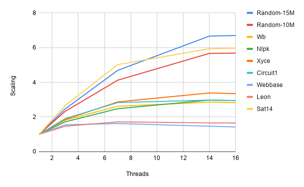
Figure 3. Strong scaling of BiPart

4.2. Scalability

Figure 3 shows the strong scaling performance of BiPart. For the largest graphs Random-10M and Random-15M, BiPart scales up to 6X with 14 threads.

Scaling is limited for the smaller hypergraphs like Webbase, Sat14 and Leon since they contain a small number of hyperedges.

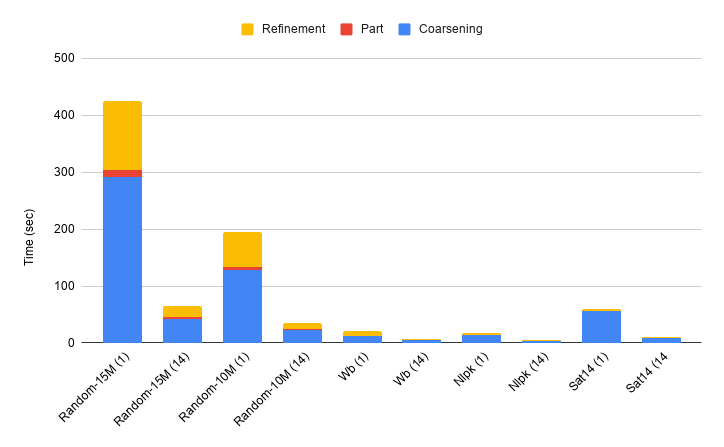
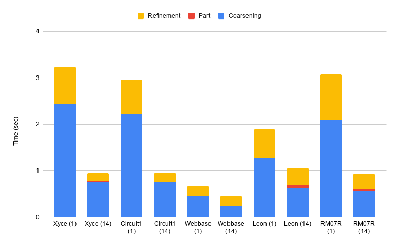
Figure 4. Runtime breakdown for BiPart on 1 thread and 14 threads.

Figure 4 shows the breakdown of the time taken by the three phases in BiPart on 1 and 14 threads, respectively. For both single thread and 14 threads, the coarsening phase takes the majority of the time for all hypergraphs.

The coarsening and refinement phases of BiPart scale similarly.

The end-to-end parallel performance of BiPart can be improved by limiting the number of levels for the coarsening phase and by a better implementation of the refinement phase. We also see a significant change in the slopes of all the scaling lines when the number of cores is increased from 7 to 8 as well as from 14 to 15. On this machine, each socket has 7 cores so the change in slope arises from NUMA effects. Improving NUMA locality is another avenue for improving the performance of BiPart.

4.3. Design-Space Exploration of Parameter Space

In this section, we discuss the effect of important tuning parameters on BiPart. The important parameters we explore are the following: the number of coarsening levels, the number of refinement iterations, and the matching policy. These parameters are described in detail in Section 3.4.

One benefit of having a deterministic system is that we can perform a relatively simple design space exploration to understand how running time and quality change with parameter settings. In this section, we discuss how the choice of these settings affects the edge cut and running time.

Figure  5 shows a sweep of the parameter space for the two hypergraphs WB and Xyce. Points corresponding to different matching policies are given different shapes; for example, triangles represent points for the LDH policy. While there are many points, we are most interested in those that are on the Pareto frontier. As mentioned in Section 3, the default settings for BiPart is to perform coarsening for at most 25 coarsening levels or as much as possible until there is no change in the size of the coarsened graph and to do two iterations of refinement per level. The BiPart points for this default setting are shown as large circles and triangles (blue in color), and we see that they both lie close to the Pareto frontier. Zoltan points are shown as black X marks; for WB, the point is far from the Pareto frontier while for Xyce, the point is on the Pareto frontier but takes much more time for a small improvement in quality.

As for the matching policy for finding a multi-node matching in the coarsening phase, there is no single policy that works best for all inputs. LDH and HDH usually dominate other policies. LWD, which has been used in HMetis, does not perform well and does not generate a point on the Pareto frontier, so it should be deprecated.

Table 4 shows the running time and quality for the default settings, for the settings that give the best quality, and for the settings that give the best running time. The default setting for BiPart is to do two iterations of refinement per level and at most 25 levels of coarsening. For the matching policy, we do not have a fixed matching policy for all graphs but it is a combination of RAND, LD, and HDH. For all hypergraphs, the point corresponding to the default setting for BiPart either lies somewhere in between the two extreme points on the Pareto frontier or lies near the Pareto frontier. We also observed that there is no unique parameter setting that guarantees for all hypergraphs that the corresponding point lies on the Pareto frontier.

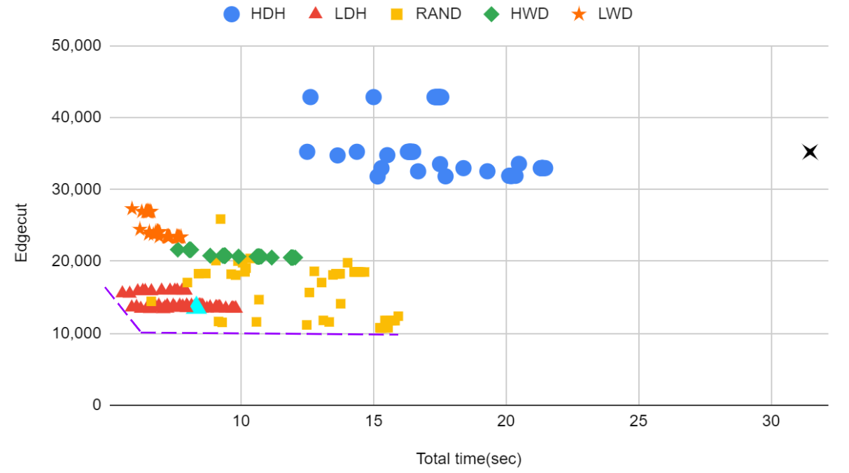
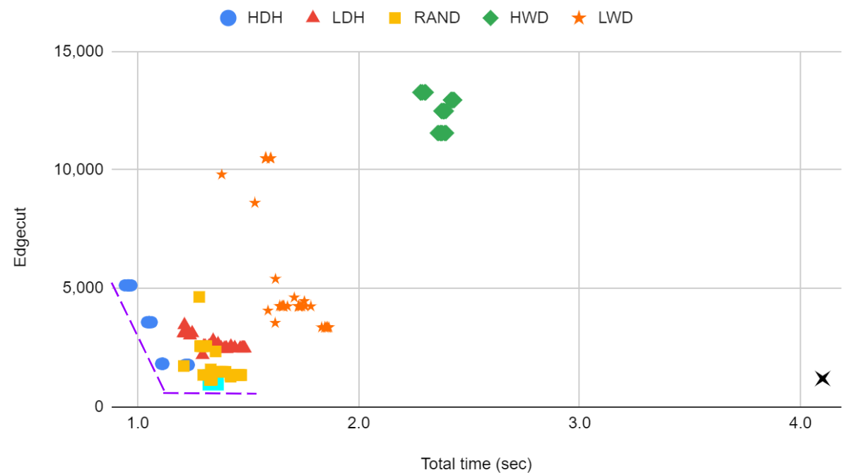
Figure 5. Design space for various tuning parameters for the two largest hypergraphs, WB (top) and Xyce (bottom); the Pareto frontier is shown for both hypergraphs

Table 4. Parameter sweep results for BiPart

	Recommended		Best Edge Cut		Best Runtime
Graph	Time (sec)	EdgeCut	Time (sec)	EdgeCut	Time (sec)	EdgeCut
Random-15M	85.4	13,968,401	71.4	13,960,994	60.7	14,000,612
Random-10M	35.2	7,588,493	35.3	7,581,745	31.4	7,618,589
WB	7.9	13,853	15.2	10,773	6.2	15,904
NLPK	5.8	98,010	5.8	88,239	4.5	121,249
Xyce	1.3	1,134	1.3	1,134	0.9	5,124
Circuit1	0.7	3,439	1.1	3,408	0.5	5,717
Webbase	0.3	624	0.4	587	0.3	622
Leon	0.9	112	2.1	60	1.5	184
Sat14	7.6	15,394	9.7	13,833	2.4	155,325
RM07R	0.8	22,350	0.9	21,601	0.6	30,207

Table 5. Performance of BiPart and KaHyPar for k-way partitioning of the IBM18 hypergraph (time in seconds)

	BiPart (14)		KaHyPar (1)
$\mathbf{k}$	Time	Edge cut	Time	Edge cut
$\mathbf{2}$	0.2	2,385	453.9	1,915
$\mathbf{4}$	0.5	5,836	425.0	2,926
$\mathbf{8}$	1.0	11,522	288.0	4,822
$\mathbf{16}$	1.6	19,116	299.5	8,560

Table 6. Performance of BiPart and KaHyPar for k-way partitioning of the WB hypergraph (time in seconds)

	BiPart (14)		KaHyPar (1)
$\mathbf{k}$	Time	Edge cut	Time	Edge cut
$\mathbf{2}$	7.9	13,853	581.5	11,457
$\mathbf{4}$	14.7	100,380	$>$ 1,800	$-$
$\mathbf{8}$	17.5	185,079	$>$ 1,800	$-$
$\mathbf{16}$	20.0	269,144	$>$ 1,800	$-$

4.4. Multiway Partitioning Performance

Figure 6 shows the scaled execution time of BiPart for multiway partitioning of the two hypergraphs Xyce and WB. For both hypergraphs, the execution times are scaled by the time taken to create 2 partitions. If $k$ is the number of partitions to be created, the critical path through the computation increases as $O(log_{2}(k))$. The experimental results shown in Figure 6 follow this trend roughly.

Tables 5 and 6 show the performance of BiPart and the current state-of-the-art hypergraph partitioner, KaHyPar, for multiway partitioning of a small graph IBM18 (Table 5) and a large graph WB (Table 6). We do not compare our results with Zoltan for $k$-way since their result is not deterministic. BiPart is much faster than KaHyPar; for example, KaHyPar times out after 30 minutes when creating 4 partitions of WB (9.8M nodes, 6.9M hyperedges), whereas BiPart can create 16 partitions of this hypergraph in just 20 seconds. However, when KaHyPar terminates in a reasonable time, it produces partitions with a better edge cut (for IBM18, the edge cut is on average 2.5X better).

We conclude that there is a tradeoff between BiPart and KaHyPar in terms of the total running time and the edge cut quality. As shown in Tables 5 and 6, BiPart may be better suited than KaHyPar for creating a large number of partitions of large graphs while maintaining determinism.

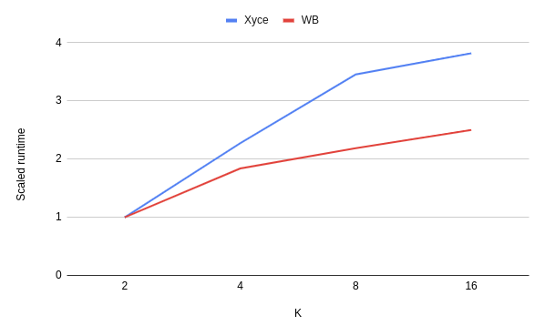
Figure 6. BiPart execution time for k-way partitioning

5. Conclusion and Future Work

We describe BiPart, a fully deterministic parallel hypergraph partitioner, and show that it significantly outperforms KaHyPar, the state-of-the-art hypergraph partitioner, in running time, albeit with lower edge-cut quality, for all inputs in our test suite. On some large graphs, which BiPart can process in less than a minute, KaHyPar takes over an hour to perform multiway partitioning.

In future work, we want to explore whether we can classify hypergraphs based on features such as the average node degree and the number of connected components to come up with optimal parameter settings and scheduling policies for a given hypergraph. We are also looking into ways to improve NUMA locality for better performance. Extending this work to distributed-memory machines might be useful for very large hypergraphs that do not fit in the memory of a single machine (Hoang et al., 2019).

- (1)
- Andreev and Räcke (2004) Konstantin Andreev and Harald Räcke. 2004. Balanced Graph Partitioning. In Proceedings of the Sixteenth Annual ACM Symposium on Parallelism in Algorithms and Architectures (Barcelona, Spain) (SPAA ’04). ACM, New York, NY, USA, 120–124. https://doi.org/10.1145/1007912.1007931
- Barnard and Simon (1993) Stephen Barnard and Horst Simon. 1993. A Fast Multilevel Implementation of Recursive Spectral Bisection for Partitioning Unstructured Problems. 711–718.
- Berge (1973) C. Berge. 1973. Graphs and Hypergraphs. Amsterdam. https://books.google.com/books?id=X32GlVfqXjsC
- Blelloch et al. (2012) Guy E Blelloch, Jeremy T Fineman, Phillip B Gibbons, and Julian Shun. 2012. Internally Deterministic Parallel Algorithms Can be Fast. In Proceedings of the 17th ACM SIGPLAN symposium on Principles and Practice of Parallel Programming. 181–192.
- Bui and Jones (1993) T N Bui and C Jones. 1993. A Heuristic for Reducing Fill-in in Sparse Matrix Factorization. (12 1993).
- Caldwell et al. (1999) Andrew E. Caldwell, Andrew B. Kahng, Andrew A. Kennings, and Igor L. Markov. 1999. Hypergraph Partitioning for VLSI CAD: Methodology for Heuristic Development, Experimentation and Reporting. In Proc. ACM/IEEE Design Automation Conf. (DAC 99), ACM. Press, 349–354.
- Çatalyürek and Aykanat (2011) Ümit Çatalyürek and Cevdet Aykanat. 2011. PaToH (Partitioning Tool for Hypergraphs). Springer US, Boston, MA, 1479–1487.
- Davis and Hu (2011) Timothy A Davis and Yifan Hu. 2011. The University of Florida sparse matrix collection. ACM Transactions on Mathematical Software (TOMS) 38, 1 (2011), 1.
- Devietti et al. (2011) Joseph Devietti, Jacob Nelson, Tom Bergan, Luis Ceze, and Dan Grossman. 2011. RCDC: A Relaxed Consistency Deterministic Computer. ACM SIGARCH Computer Architecture News 39, 1 (2011), 67–78.
- Devine et al. (2006a) Karen D. Devine, Erik G. Boman, Robert T. Heaphy, Rob H. Bisseling, and Umit V. Catalyurek. 2006a. Parallel Hypergraph Partitioning for Scientific Computing. In Proceedings of the 20th International Conference on Parallel and Distributed Processing (Rhodes Island, Greece) (IPDPS’06). IEEE Computer Society, Washington, DC, USA, 124–124. http://dl.acm.org/citation.cfm?id=1898953.1899056
- Devine et al. (2006b) Karen D. Devine, Erik G. Boman, Robert T. Heaphy, Rob H. Bisseling, and Umit V. Catalyurek. 2006b. Parallel Hypergraph Partitioning for Scientific Computing. IEEE.
- Fiduccia and Mattheyses (1982) C. M. Fiduccia and R. M. Mattheyses. 1982. A Linear-Time Heuristic for Improving Network Partitions. In 19th Design Automation Conference. 175–181.
- Fiedler (1973) M. Fiedler. 1973. Algebraic Connectivity of Graphs. Czech. Math. J. 23 (1973), 298–305.
- Grover and Leskovec (2016) Aditya Grover and Jure Leskovec. 2016. node2vec: Scalable Feature Learning for Networks. In Proceedings of the 22nd ACM SIGKDD international conference on Knowledge discovery and data mining. 855–864.
- Hendrickson et al. (1995) Bruce Hendrickson, Bruce Hendrickson, and Robert Leland. 1995. A Multilevel Algorithm for Partitioning Graphs. In Proceedings of the 1995 ACM/IEEE Conference on Supercomputing (San Diego, California, USA) (Supercomputing ’95). ACM, New York, NY, USA, Article 28. https://doi.org/10.1145/224170.224228
- Heuer et al. (2019) Tobias Heuer, Peter Sanders, and Sebastian Schlag. 2019. Network Flow-Based Refinement for Multilevel Hypergraph Partitioning. ACM J. Exp. Algorithmics 24, 1, Article 2.3 (Sept. 2019), 36 pages. https://doi.org/10.1145/3329872
- Hoang et al. (2019) L. Hoang, R. Dathathri, G. Gill, and K. Pingali. 2019. CuSP: A Customizable Streaming Edge Partitioner for Distributed Graph Analytics. In 2019 IEEE International Parallel and Distributed Processing Symposium (IPDPS). 439–450. https://doi.org/10.1109/IPDPS.2019.00054
- Hower et al. (2011) Derek R Hower, Polina Dudnik, Mark D Hill, and David A Wood. 2011. Calvin: Deterministic or Not? Free Will to Choose. In 2011 IEEE 17th International Symposium on High Performance Computer Architecture. IEEE, 333–334.
- Kabiljo et al. (2017) Igor Kabiljo, Brian Karrer, Mayank Pundir, Sergey Pupyrev, and Alon Shalita. 2017. Social Hash Partitioner: A Scalable Distributed Hypergraph Partitioner. Proc. VLDB Endow. 10, 11 (Aug. 2017), 1418–1429. https://doi.org/10.14778/3137628.3137650
- Kaler et al. (2016) Tim Kaler, William Hasenplaugh, Tao B Schardl, and Charles E Leiserson. 2016. Executing Dynamic Data-graph Computations Deterministically Using Chromatic Scheduling. ACM Transactions on Parallel Computing (TOPC) 3, 1 (2016), 1–31.
- Karypis et al. (1999) George Karypis, Rajat Aggarwal, Vipin Kumar, and Shashi Shekhar. 1999. Multilevel Hypergraph Partitioning: Applications in VLSI Domain. IEEE Trans. Very Large Scale Integr. Syst. 7, 1 (March 1999), 69–79.
- Karypis and Kumar (1998) George Karypis and Vipin Kumar. 1998. A Fast and High Quality Multilevel Scheme for Partitioning Irregular Graphs. SIAM J. Sci. Comput. 20, 1 (Dec. 1998), 359–392.
- Kernighan and Lin (1970) B. W. Kernighan and S. Lin. 1970. An efficient heuristic procedure for partitioning graphs. The Bell System Technical Journal 49, 2 (Feb 1970), 291–307.
- library ([n.d.]) Boost library. [n.d.]. Boost C++ Libraries. https://www.boost.org/users/history/version_1_67_0.html
- Maleki and Burtscher (2018) Sepideh Maleki and Martin Burtscher. 2018. Automatic Hierarchical Parallelization of Linear Recurrences. SIGPLAN Not. 53, 2 (March 2018), 128–138. https://doi.org/10.1145/3296957.3173168
- Mayer et al. (2018) Christian Mayer, Ruben Mayer, Sukanya Bhowmik, Lukas Epple, and Kurt Rothermel. 2018. HYPE: Massive Hypergraph Partitioning with Neighborhood Expansion. CoRR abs/1810.11319 (2018). arXiv:1810.11319
- Miller et al. (1991) Gary L. Miller, Shang-Hua Teng, and Stephen A. Vavasis. 1991. A Unified Geometric Approach to Graph Separators. In Proceedings of the 32nd Annual Symposium on Foundations of Computer Science (SFCS ’91). IEEE Computer Society, USA, 538–547. https://doi.org/10.1109/SFCS.1991.185417
- Mitchell (1997) T.M. Mitchell. 1997. Machine Learning. McGraw-Hill. https://books.google.com/books?id=EoYBngEACAAJ
- Neto et al. (2019) W. Lau Neto, M. Austin, S. Temple, L. Amaru, X. Tang, and P.-E. Gaillardon. 2019. LSOracle: A Logic Synthesis Framework Driven by Artificial Intelligence. In IEEE/ACM International Conference on Computer-Aided Design (ICCAD).
- Nguyen et al. (2013) Donald Nguyen, Andrew Lenharth, and Keshav Pingali. 2013. A Lightweight Infrastructure for Graph Analytics. In Proceedings of the Twenty-Fourth ACM Symposium on Operating Systems Principles (Farminton, Pennsylvania) (SOSP ’13). ACM, New York, NY, USA, 456–471.
- Nguyen et al. (2014) Donald Nguyen, Andrew Lenharth, and Keshav Pingali. 2014. Deterministic Galois: On-demand, Portable and Parameterless. In Proceedings of the 19th International Conference on Architectural Support for Programming Languages and Operating Systems (ASPLOS ’14).
- Perozzi et al. (2014) Bryan Perozzi, Rami Al-Rfou, and Steven Skiena. 2014. Deepwalk: Online Learning of Social Representations. In Proceedings of the 20th ACM SIGKDD international conference on Knowledge discovery and data mining. 701–710.
- Pingali et al. (2011a) Keshav Pingali, Donald Nguyen, Milind Kulkarni, Martin Burtscher, Muhammad Amber Hassaan, Rashid Kaleem, Tsung-Hsien Lee, Andrew Lenharth, Roman Manevich, Mario Méndez-Lojo, Dimitrios Prountzos, and Xin Sui. 2011a. The Tao of Parallelism in Algorithms. In PLDI 2011. 12–25.
- Pingali et al. (2011b) Keshav Pingali, Donald Nguyen, Milind Kulkarni, Martin Burtscher, M. Amber Hassaan, Rashid Kaleem, Tsung-Hsien Lee, Andrew Lenharth, Roman Manevich, Mario Méndez-Lojo, Dimitrios Prountzos, and Xin Sui. 2011b. The TAO of parallelism in algorithms. In Proc. ACM SIGPLAN Conf. Programming Language Design and Implementation (San Jose, California, USA) (PLDI ’11). 12–25. https://doi.org/10.1145/1993498.1993501
- Pothen et al. (1990) A. Pothen, H. Simon, and K.-P. Liou. 1990. Partitioning Sparse Matrices with Eigenvectors of Graphs. SIAM J. Matrix Anal. Appl. 11 (1990), 430–452.
- Qu et al. (2015) G. Qu, Z. Fang, J. Zhang, and S. Zheng. 2015. Switch-Centric Data Center Network Structures Based on Hypergraphs and Combinatorial Block Designs. IEEE Transactions on Parallel and Distributed Systems 26, 4 (April 2015), 1154–1164. https://doi.org/10.1109/TPDS.2014.2318697
- Trifunović and Knottenbelt (2008) Aleksandar Trifunović and William J. Knottenbelt. 2008. Parallel Multilevel Algorithms for Hypergraph Partitioning. J. Parallel Distrib. Comput. 68, 5 (May 2008), 563–581.
- Xia et al. (2015) F. Xia, A. M. Ahmed, L. T. Yang, and Z. Luo. 2015. Community-Based Event Dissemination with Optimal Load Balancing. IEEE Trans. Comput. 64, 7 (July 2015), 1857–1869. https://doi.org/10.1109/TC.2014.2345409
- Yang et al. (2016) Wenyin Yang, Guojun Wang, Li Ma, and Shiyang Wu. 2016. A Distributed Algorithm for Balanced Hypergraph Partitioning. In Advances in Services Computing, Guojun Wang, Yanbo Han, and Gregorio Martínez Pérez (Eds.). Springer International Publishing, Cham, 477–490.