Dynamical Properties and Effects of Quantum Diffraction on The Propagation of E-A-Solitary Waves in Three-Component Fermi Plasma

Abstract

Electron Acoustic Solitary structures in Fermi Plasma with two temperature electrons have various applications in space and laboratory-made plasma. Formulation of an adequate theory is important to understand various physical systems with various physical parameters. The motion of two temperature electrons in a quantum Fermi plasma system highly affects the solitary profile of the system. We study the quantum Fermi plasma system with two temperature electrons where the streaming velocities of the two-electron population are opposite. We consider the quantum hydrodynamic model (QHD) and derive a linear dispersion relation for the system. For the non-linear study of the system, we use the standard perturbation technique to derive KdV-B equation and show the evolution of a solitary profile with different plasma parameters. We analyze the stable Rouge wave structure using NLSE and show simulation results. We study the dynamical properties and phase plot for a two-stream quantum Fermi plasma system with two temperature electrons.

I Introduction

Plasma systems containing two distinct groups of electrons shows Electron acoustic waves (EAWs). The distinction between two electron groups comes from their energy. Two types of electrons are 1) Hot electrons and 2) Cold electrons. The frequency of electron acoustic mode is higher than ion acoustic frequencies of plasmas. Hot electrons can freely move with less viscous drag and supply restoring force, whereas cold electron feels viscous drag and produce inertia to the system. The thermal speed of hot electron is very large in comparison to cold electron. The phase speed of electron acoustic wave is smaller than the thermal speed of hot electrons but much larger than thermal speed of cold electrons. In this system ions may be considered as uniform neutralizing background. EAWs with two groups of electrons plays an important role in space plasma (Ang and Zhang (2007)Ang. L.K. (2007); Barnes et al. (2003)Barnes et al. (2003); Feldman et al. (1975)Feldman et al. (1975), (1983a)Feldman et al. (1983) as well as laboratory made plasmas (Ditmire et al. (1998)Ditmire et al. (1998); Sheridan et al. (1991)Gudmundsson et al. (2002); Armstrong et al. (1979)Armstrong R.J. (1979); Kadomtsev and Pogutse (1971)Kadomtsev and Pogutse (1971); Henry and Trguier (1972)Henry and Trguier (1972); Defler and Simonen (1969)Saberian and Esfandyari-Kalejahi (2014)). The source of broadband electrostatic noises can be addressed with EAWs and it has been used to explain those. The wave emission in different regions of earth’s atmosphere can be explained with EAWs. For these studies EAWs has become one of the important research areas in plasma physics. In recent years there is a boost in the study of the nonlinear evolution of EAWs (Bains et al. (2011)Bains et al. (2011); Soultana and Kourakis (2011)Sultana and Kourakis (2011); Kourakis and Shukla (2004)Kourakis and Shukla (2004); Singh and Lakhina (2001)Singh and Lakhina (2001)). Various space-craft missions, e,g, the FAST at the auroral region (Ergun et al. (1998aErgun et al. (1998a), 1998bErgun et al. (1998b)); Delory et al. (1998)Delory et al. (1998); Pottelette et al. (1999)Pottelette et al. (1999)) and the POLAR and GEOTAIL missions in the magnetosphere (Matsumoto et al. (1994)Matsumoto et al. (1994); Franz et al. (1998)Franz et al. (1998); Cattell et al. (2003)Cattell et al. (2003)) explained by EAW related structures. Most of these application sites need theory and better understanding of non-relativistic classical plasmas. However, there are numbers of works on the theory of nonlinear propagation of electrostatic modes in quantum plasmas with consideration of quantum hydrodynamic model of plasma (Shukla and Eliasson (2006)Shukla and Eliasson (2006); Sahu and Roychoudhury (2006)Sahu and Roychoudhury (2006); Ali and Shukla (2006)Shukla and Ali (2005); Manfredi (2005)Manfredi (2005); Haas et al. (2003)Haas et al. (2003); Gardner and Ringhofer (1996)Mamun and Shukla (2010)). The non-linear wave structure of cold and hot electrons are investigated Chandra et al. (2013)-Chandra and Ghosh (2012)

In this paper we study linear and nonlinear properties of EAWs in Fermi plasma with two temperature electrons. We first assume basic hydrodynamic equations for the system then we normalize them using suitable scaling for the system. With the normalized equations on hand we linearize them to get linear dispersion relation and linear dispersion characteristics are investigated. The Korteweg-de Vries Burgers (KdV-B) equation is derived using standard perturbation technique. We investigate dependence of soliton properties on different plasma parameters. We study Rouge wave formation for the system. We investigate the dynamical nature of the system. Then we conclude the paper with some remarks and future work plans.

II Basic Formulation

The plasma system that we considered is unmagnetized consisting of two groups of electrons. Two groups are 1) Hot electrons and 2) Cold electrons. The thermal energy of hot electron is higher than cold electrons so the mobility of hot electron is large compared to that of cold electrons. So, in the momentum equation for hot electron we consider inertia term as zero, whereas in the momentum equation of cold electrons we consider a viscous term as its mobility is less and more responsive to the viscous forces.

$$\frac{\partial n_{h}}{\partial t}+\frac{\partial\left(n_{h}u_{h}\right)}{\partial x}=0$$ (1)

$$\frac{\partial n_{c}}{\partial t}+\frac{\partial\left(n_{c}u_{c}\right)}{\partial x}=0$$ (2)

$$0=\frac{e}{m_{e}}\frac{\partial\phi}{\partial x}-\frac{1}{m_{e}n_{h}}\frac{\partial P_{h}}{\partial x}+\frac{\hbar^{2}}{2m_{e}\gamma^{2}_{h}}\frac{\partial}{\partial x}\left[\frac{1}{\sqrt{n_{h}}}\frac{\partial^{2}\sqrt{n_{h}}}{\partial x^{2}}\right]$$ (3)

This is momentum equation for hot electrons. The inertia term (left hand side of the equation) is zero, as hot electrons are very mobile so its inertia can be assumed to be zero. Here, $\gamma_{h}=\left(1-\frac{u_{h}^{2}}{c^{2}}\right)^{-\frac{1}{2}}$

$$\left(\frac{\partial}{\partial t}+u_{c}\frac{\partial}{\partial x}\right)(u_{c}\gamma_{c})=\frac{e}{m_{e}}\frac{\partial\phi}{\partial x}\\ -\frac{1}{m_{e}n_{c}}\frac{\partial P_{c}}{\partial x}+\frac{\hbar^{2}}{2m_{e}^{2}\gamma_{c}^{2}}\frac{\partial}{\partial x}\left[\frac{1}{\sqrt{n_{c}}}\frac{\partial^{2}\sqrt{n_{c}}}{\partial x^{2}}\right]\\ +\eta_{c}\frac{\delta^{2}u_{c}}{\delta x^{2}}$$ (4)

This is momentum equation for cold electrons. The inertia term is non zero as the mobility of cold electrons is very less. For our two-electron plasma system cold electron produces the restoring force for electron-acoustic oscillations. Cold electrons also got a viscous term. Here, $\gamma_{c}=\left(1-\frac{u_{c}^{2}}{c^{2}}\right)^{-\frac{1}{2}}$

$$\frac{\partial^{2}\phi}{\partial x^{2}}=4\pi e\left(n_{c}+n_{h}-Z_{i}n_{i}\right)$$ (5)

The subscript $i$ in the Poisson’s equation is for representing ions. The above-mentioned equations are the governing equations for the plasma system, where $n_{h}$ and $n_{c}$ are the density of hot and cold electrons respectively. $\phi$ is the electrostatic potential. $P_{h}$ is the pressure law for hot electrons. $\hbar$ is the plank constant divided by $2\pi$. $m_{e}$ is the mass of electron and $e$ is the charge of electron and $\eta_{c}$ is the viscous constant for cold electrons.

We considered Fermi pressure as the main pressure component for electrons. Fermi pressure is

$$P_{j}=\frac{m_{j}V_{Fj}^{2}}{3n_{j0}^{2}}n_{j}^{3}$$ (6)

where subscript $j=h$ is for hot electrons and $j=c$ for cold electrons. $n_{h0}$ is the initial hot electron density. The parameters need to be normalized to get a good control of the equations and normalized equations are easy to work with. Normalization means we need to define some suitable scaling associated with our problem. With these scaling constants we can make our parameters dimensionless.

For our problem, normalization has been done in following ways $x\rightarrow x\omega_{j}/V_{Fj},t\rightarrow t\omega_{j},\phi\rightarrow e\phi/2k_{B}T_{Fj},n_{h}\rightarrow n_{h}/n_{h0},n_{c}\rightarrow n_{c}/n_{c0},,u_{h}\rightarrow u_{h}/V_{Fh},u_{c}\rightarrow u_{c}/V_{Fc}$ where $\omega_{j}=\sqrt{4\pi en_{c0}e^{2}/m_{e}}$, $V_{Fh}=\sqrt{\frac{2K_{B}T_{Fh}}{m_{e}}}$ and $H=\hbar\omega_{j}/2k_{B}T_{Fj}$ Changing the variables and parameters accordingly we have Normalized Governing Equations.

$$\frac{\partial n_{h}}{\partial t}+\frac{\partial\left(n_{h}u_{h}\right)}{\partial x}=0$$ (7)

$$\frac{\partial n_{c}}{\partial t}+\frac{\partial\left(n_{c}u_{c}\right)}{\partial x}=0$$ (8)

$$0=\frac{\partial\phi}{\partial x}-n_{h}\frac{\partial n_{h}}{\partial t}+\frac{H^{2}}{2\gamma_{h}^{2}}\frac{\partial}{\partial x}\left[\frac{1}{\sqrt{n_{h}}}\frac{\partial^{2}\sqrt{n_{h}}}{\partial x^{2}}\right]$$ (9)

$$\left(\frac{\partial}{\partial t}+u_{c}\frac{\partial}{\partial x}\right)(u_{c}\gamma_{c}) =\frac{\partial\phi}{\partial x}$$ (10)

$$+\frac{H^{2}}{2\gamma_{c}^{2}}\frac{\partial}{\partial x}\left[\frac{1}{\sqrt{n_{c}}}\frac{\partial^{2}\sqrt{n_{c}}}{\partial x^{2}}\right]$$

$$+\eta_{c}\frac{\delta^{2}u_{c}}{\delta x^{2}}$$

$$\frac{\partial^{2}\phi}{\partial x^{2}}=n_{c}+\frac{n_{h}}{\delta}-\frac{\delta_{i}}{\delta}n_{i}$$ (11)

where $\delta=\frac{n_{c0}}{n_{h0}}$, $\delta_{1}=Z_{i}\frac{n_{i0}}{n_{h0}}$.

III Linear Dispersion Relation

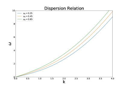
Figure 1: Dispersion relation plot for different $u_{0}$ keeping $\delta=0.3$ and $H=1$

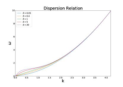
Figure 2: Dispersion relation plot for different $\delta$ keeping $u_{0}=0.25$ and $H=1$

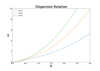
Figure 3: Dispersion relation plot for different $H$ keeping $\delta=0.3$ and $u_{0}=0.25$

The system parameters can be expanded into following perturbation expansion for $n_{h}$, $n_{c}$, $u_{h}$, $u_{c}$, and $\phi$

$$\left(\begin{array}[]{l}n_{j}\\ u_{j}\\ \phi\end{array}\right)=\left(\begin{array}[]{c}1\\ \pm u_{0j}\\ \phi_{0}\end{array}\right) +\epsilon^{1}\left(\begin{array}[]{l}n_{j}^{(1)}\\ u_{j}^{(1)}\\ \phi^{(1)}\end{array}\right)+\epsilon^{2}\left(\begin{array}[]{l}n_{j}^{(2)}\\ u_{j}^{(2)}\\ \phi^{(2)}\end{array}\right)$$ (24)

$$+\epsilon^{3}\left(\begin{array}[]{l}n_{j}^{(3)}\\ u_{j}^{(3)}\\ \phi^{(3)}\end{array}\right)+\cdots$$ (28)

Here we assume existence of streaming velocities for hot and cold electrons (+ve for hot electron and -ve for cold electrons) and equilibrium field in constant field $\phi_{0}$. Substituting these expansions in the governing relations and then taking only linear terms (linearizing) with the assumption that all field variable varies periodically as $e^{i(kx-\omega t)}$, we have following complex dispersion relation

$$-k^{2}=\frac{1}{\left[\frac{H^{2}k^{2}}{4}\gamma_{c}^{2}-\left(\frac{\omega-u_{0}k}{k}\right)^{2}\right]+i\eta_{c}\left(\omega-u_{0}k\right)}\\ +\frac{\frac{1}{\delta}}{1+\frac{H^{2}k^{2}}{4}\gamma_{c}^{2}}$$ (29)

Here we assume $u_{0h}=u_{0c}=u_{0}.$ Now we have to keep in mind that $k$ itself is a complex number, $k=$ $k_{1}+ik_{2}$. Putting this into the expression of Complex dispersion relation we have two equations, one for real part of the equation and other for imaginary part of the equation. The real dispersion equation is:

$$-1=\frac{\left(\frac{1}{\delta}+k_{1}^{2}+\frac{H^{2}k_{1}^{4}}{4}\gamma_{c}^{2}\right)\cdot\left[\frac{H^{2}k_{1}^{4}}{4}\gamma_{c}^{2}-\omega^{2}-u_{0}^{2}k_{1}^{2}+2\omega u_{0}k_{1}\right]}{\left[k_{1}^{2}+\frac{H^{2}k_{1}^{2}}{4}\gamma_{c}^{2}\right]}$$ (30)

With $k_{2}=0,$ if we plot $\omega$ vs $k_{1}$ then the plot will give us dispersion plot. $H,u_{0},\delta$ are the parameters of the equation.

Fig. 1 shows dispersion plot for different values of equilibrium streaming velocity $u_{0}.$ Plot shows with increasing $u_{0}$ the slope of $\omega$ vs $k$ plot increases, i.e. an increase in EAW velocity.

Fig. 2. shows dispersion plot for different values of $\delta.$ Increase in $\delta$ shows decrease in slope (for small $\omega$ this behavior is clear). For $\delta=1$ i.e. the density of hot and cold electrons are same, we are getting a linear behaviour in small $k$ regime.

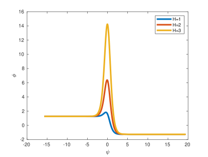
Figure 4: 2D Solitary profile for different $H$ keeping $\delta$ and $u_{0}$ constant

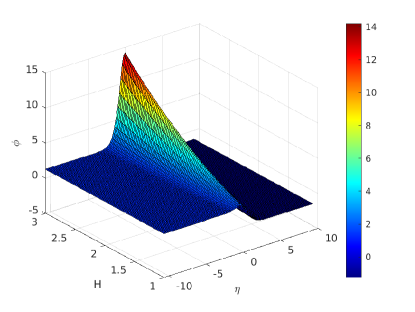
Figure 5: 3D Solitary profile for different $H$ keeping $\delta$ and $u_{0}$ constant

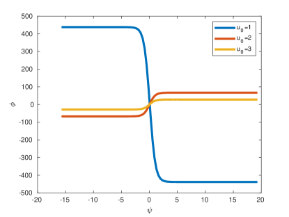
Figure 6: 2D Solitary profile for different $u_{0}$ keeping $\delta$ and $H$ constant

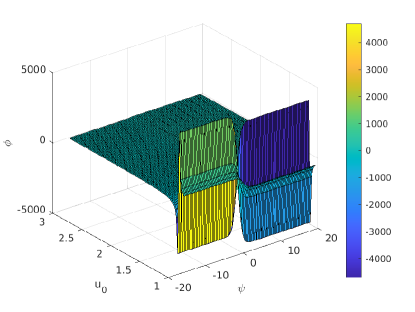
Figure 7: 3D Solitary profile for different $u_{0}$ keeping $\delta$ and $H$ constant

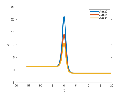
Figure 8: 2D Solitary profile for different $\delta$ keeping $H$ and $u_{0}$ constant

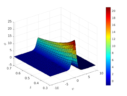
Figure 9: 3D Solitary profile for different $\delta$ keeping $H$ and $u_{0}$ constant

Increasing delta means more initial cold electrons compare to hot electrons. So, according to our plots a greater number of initial cold electrons implies a decrease in $k$ vs $\omega$ slop, that is increase in EAW velocity. Velocity of sound waves, rather acoustic waves increases with increasing the rigidity of the medium. Now a greater number of cold electrons means more viscous drag and eventually more rigid medium, which can be the cause for increase in EAW velocity.

Fig. 3. shows $\omega$ vs $k$ plot for different $H$ values. We change $H$ from 1 to 3 keeping $u_{0},\delta$ and constant. As $H$ increases the slope of $\omega$ vs $k$ plot increases, that is also visible from the dispersion relation. However, $H$ depends on plasma frequency $\omega_{c}$ linearly. So, higher $H$ means higher plasma frequency. This leads to a conclusion that for high plasma frequency the EAW has less wavenumber with same frequency.

IV Korteweg-de Vries Burgers Equation for Nonlinear Study

We used standard reductive perturbation technique with usual stretching of space and time variables. We used two perturbation expansions to see the behavior of the solution of KdV-B equation. Using the perturbation expansion eq. (24) and, stretching of variables

$$\xi=\epsilon^{\frac{1}{2}}\left(x-v_{0}t\right);\quad\eta=\eta_{0}\epsilon^{\frac{1}{2}};\quad\text{and}\quad\tau=\epsilon^{\frac{3}{2}}t$$ (31)

Putting them into governing equations and taking the lower order terms with power of epsilon we have the following KdV-Burger equation

$$\frac{\partial\phi}{\partial\tau}+A\phi\frac{\partial\phi}{\partial\xi}+B\frac{\partial^{3}\phi}{\partial\xi^{3}}-C\frac{\partial^{2}\phi}{\partial\xi^{2}}=0$$ (32)

The solution to (32) is

$$\phi=\frac{12D}{N}\operatorname{sech}^{2}\xi-\frac{36R}{15N}\tanh\xi$$ (33)

with,

$$A=\frac{2DS_{1}R_{1}+Fn_{0c}R_{1}^{2}-D\left(M-u_{0c}\right)\frac{Q_{1}^{2}}{n_{0h}\delta}}{DS_{1}+n_{0c}R_{1}\left(1+\frac{3u_{0c}^{2}}{2c^{2}}\right)}$$ (34)

$$B=\frac{\left(D\left(M-u_{0c}\right)\left(\frac{T_{h}Q_{1}}{n_{0}h^{\delta}}\right)-T_{c}S_{1}n_{0c}-D\left(M-u_{0c}\right)\right)}{DS_{1}+n_{0c}R_{1}\left(1+\frac{3u_{0c}^{2}}{2c^{2}}\right)}$$ (35)

$$C=\eta_{c}R_{1}$$ (36)

With,

$$D=M+\frac{3Mu_{0c}^{2}}{2c^{2}}-\frac{3u_{0c}^{3}}{2c^{2}}-u_{0c}$$ (37)

$$F=1+\frac{9u_{0c}^{2}}{2c^{2}}-\frac{3Mu_{0c}}{c^{2}}$$ (38)

$$T_{c}=\frac{H^{2}}{4n_{oc}^{2}}\left(1-\frac{u_{0c}^{2}}{c^{2}}\right)$$ (39)

$$T_{h}=\frac{H^{2}}{4n_{0h}^{2}}\left(1-\frac{u_{0h}^{2}}{c^{2}}\right)$$ (40)

$$S_{1}=\frac{n_{0c}}{\left.\left(M-u_{0c}\right)\left(u_{0c}+\frac{3u_{0c}^{3}}{2c^{2}}\right)-M\left(1+\frac{3u_{0c}^{2}}{2c^{2}}\right)\right]}$$ (41)

$$R_{1}=\frac{1}{\left(u_{0c}+\frac{3u_{0}^{3}c}{2c^{2}}\right)-M\left(1+\frac{3u_{0}^{2}c}{2c^{2}}\right)}$$ (42)

$$Q_{1}=\frac{1}{n_{0k}}$$ (43)

$\text{ For, }n_{0j}=1;u_{0j}=0;j=hc$

$S_{1}=-\frac{1}{M^{2}};R_{1}=-\frac{1}{M};Q_{1}=1;D=M;F=1;T=\frac{H^{2}}{4}$

The the value of

$$A=\left(\frac{M^{3}}{2\delta}-\frac{3}{2M}\right)$$ (44)

$$B=\left(\frac{H^{2}}{8M}+\frac{M^{3}}{3}-\frac{M^{3}H^{2}}{4\delta}\right)$$ (45)

$$C=-\frac{\eta_{0}}{M}$$ (46)

FIG.4 and FIG.5 shows an increase in the peak of the solitary profile with increasing $H$ For this plot $u_{0}$=0.5 and $\delta$=0.45. FIG.7 and FIG.8 show decrease in the peak of the solitary profile with increasing $\delta$. For this plot $u_{0}$=0.5 and $H$=2

V Rogue wave

KdV-B equation gives the solitary wave structures which are created due to the balance between the dispersive force and non-linear force in plasma. In case the balance breaks the KdV-B starts to modify itself to a sudden wave having amplitude almost twice or greater than the amplitude of normal waves at that time. Like the sudden high amplitude, the suddenness of its timing makes it more dangerous. The study of the Rogue wave is important as the interference of the waves from different directions and the non-linear property make it unpredictable. We study the stability of Rogue wave and its evolution from our KdV-B equation

$$F=\epsilon^{2}F_{0}+\sum_{s=1}^{\infty}\epsilon_{s}\left(F_{s}e^{is\psi}+F_{s}^{*}e^{-is\psi}\right)$$ (47)

Where, $F$ is the field variable, is the smallness parameter, and $\psi$ is the phase factor. Now, using this equation we can expand the field variable i.e. the potential in KdV-B equation

$$\phi=\epsilon^{2}\phi_{0}+\epsilon\phi_{1}e^{i\psi}+\epsilon\phi_{1}^{*}e^{-i\psi}+\epsilon^{2}\phi_{2}e^{2i\psi}+\epsilon^{2}\phi_{2}^{*}e^{-2i\psi}+\cdots$$ (48)

The first harmonics ($\phi_{1}$) and second harmonics ($\phi_{2}$) can be further expanded respectively

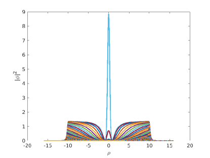
Figure 10: Rogue wave structure

$$\phi_{1}=\phi_{1}^{(1)}+\epsilon\phi_{1}^{(2)}+\epsilon^{2}\phi_{1}^{(3)}+\ldots$$ (49)

$$\phi_{2}=\phi_{2}^{(1)}+\epsilon\phi_{2}^{(2)}+\epsilon^{2}\phi_{2}^{(3)}+\ldots$$ (50)

$F_{0}$ and $F_{s}$ are assumed to vary very slowly with space and time. Now, we use the change in variables $\frac{\partial}{\partial\tau}=-is\omega-\epsilon c\frac{\partial}{\partial\rho}+\epsilon^{2}\frac{\partial}{\partial\theta}\text{ and }\frac{\partial}{\partial\xi}=isk+\epsilon\frac{\partial}{\partial\rho}$ and put it in the Eq. (32) and equate the coefficients of the first order of $\epsilon$, we get

$$\omega=-Bk^{3}$$ (51)

$$\frac{d\omega}{dk}=-3Bk^{2}$$ (52)

Equating the coefficients of $e^{2i\psi}$ with $\epsilon^{2}$

$$\varphi_{2}^{(1)}=\frac{A}{6Bk^{2}}\varphi_{1}^{(1)^{2}}$$ (53)

Equating the terms independent of $\psi$ with $\epsilon^{3}$

$$\varphi_{0}^{(1)}=\frac{A}{C}\varphi_{1}^{(1)}\varphi_{1}^{(1)^{*}}$$ (54)

By equating the other higher terms we get

$$\frac{\partial\varphi_{1}^{(1)}}{\partial\tau}+3ikB\frac{\partial^{2}\varphi_{1}^{(1)}}{\partial\rho^{2}}=-iAk\left(\varphi_{0}^{(1)}\varphi_{1}^{(1)}+\varphi_{2}^{(1)}\varphi_{1}^{(1)^{*}}\right)$$ (55)

$$i\frac{\partial\varphi_{1}^{(1)}}{\partial\tau}-3kB\frac{\partial^{2}\varphi_{1}^{(1)}}{\partial\rho^{2}}+\frac{A^{2}}{6Bk}\left(\varphi_{1}^{(1)^{2}}\varphi_{1}^{(1)^{*}}\right)=0$$ (56)

Let’s assume $P=ic-3Bk$ and $Q=A^{2}k\left[\frac{1}{6Bk^{2}+4ikc}-\frac{1}{3Bk^{2}}\right].$ The term $\mathrm{PQ}$ is very important in defining the existence of a rogue wave. In the region $PQ<0$ the rogue wave is stable and for $PQ>0$ the rogue wave doesn’t exist. The solution of Eq. (56) we get as

$$\phi(\rho,\theta)=\sqrt{\frac{2P}{Q}}\left[\frac{4(1+4iPQ)}{1+16P^{2}Q^{2}+4\rho^{2}}-1\right]\exp(2iP\theta)$$ (57)

Here we plot the potential amplitude with the changed variable $\rho$ for different values of $\theta$. And we take almost 500 values of $\theta$ and as one can see that for only one value the potential suddenly gets abnormally high with respect to the other. All of the solutions we get from the same NLSE, where only one wave behaves dangerously. It perfectly depicts the feature of a Rogue Wave, the amplitude is way higher than that of solitary profiles in Fig. (4) to Fig. (9).

Here we take the viscosity coefficient $\eta_{c}=5$ and observed that the amplitude of the rogue wave in the plot is lower than that of the rogue wave with no viscous term.

VI Simulation of KdV-B and Rouge wave evolution

The static plots of two simulations of the solitary profiles and rogue wave profile of the relativistic plasma are shown below.

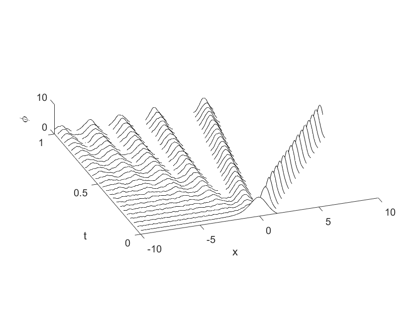
Figure 11: Simulation result of evolution of solitary profile

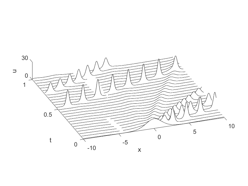
Figure 12: Simulation result of evolution of Rogue wave profiles

A movie of KdV-B evolution can be found in this link: https://doi.org/10.5281/zenodo.4366748 and a movie of Rouge wave evolution can be found in this link: https://doi.org/10.5281/zenodo.4384499 .

In both FIG.11 and FIG.12, using the solutions of KdV-B and rouge wave, we simulate the KDV solitary wave and rogue wave respectively. Here, $‘x’$ represents the space coordinate and $‘t’$ represents the time coordinate, and $‘u’$ is the amplitude. In both cases, we see the changes in the waves in the interval between $t=0s$ and $t=1s$. As you can see from the simulations that rogue waves have much higher amplitudes than those of normal solitary waves and also less frequent than normal waves.

VII Dynamical Study

To get the phase diagram of EAWs, we study a travelling wave solution followed by the KdV-B equation. To do that we use the transformation $\eta=$ $\xi-M\tau$ with the proper boundary conditions at $\eta\rightarrow$ $\pm\infty,\psi,\delta\psi/\delta\eta$ and $\left(\delta^{\wedge}2\psi\right)/\left(\delta\eta^{\wedge}2\right)\rightarrow 0$ where $M$ is the velocity of the wave. Applying a transformation like Abdikian et al. (2020) we can write the Non-linear Schrodinger equation as

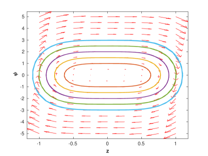
Figure 13: $\psi$ vs $z$ plot (Phase plot) for dynamical behaviour.

$$\frac{d^{2}\psi}{d\eta^{2}}=\left(\beta^{2}-\frac{1}{M_{1}l^{2}}\beta V\right)\psi-\frac{M_{2}}{M_{1}l^{2}}$$ (58)

Eq. (41) can be written in the following dynamical form

$$\frac{d\psi}{d\eta}=z$$ (59)

$$\frac{dz}{d\eta}=M_{1}\psi-M_{2}\psi^{3}$$ (60)

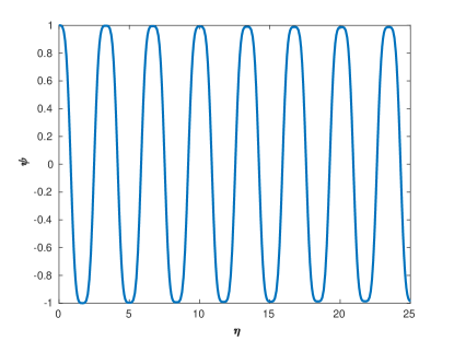
Figure 14: $\psi$ vs $\eta$ plot for dynamical behaviour.

The phase plot gives the dynamical nature of the system (Fig.13) The progressive nature of EAW can be seen from Fig.14. Plot shows a stable solution. Different coloured plots in phase diagram correspond to different energy solutions. Green one is the highest energy and blue one is the lowest.

VIII summary

Both the linear and nonlinear properties of electron-acoustic wave (EAW) have been investigated in three component Fermi plasma consisting of two of Fermi pressure for hot electrons. The stable models for EAWs are shown. The dependence of electron-acoustic wave velocity on different plasma parameters is shown and explained. The slope of the dispersion relation plots depends on the velocity of EAW inversely. The dependence of this EAW velocity and EAW frequency on different plasma parameters has been shown. Electron-acoustic wave velocity increases with increasing $H$, $u_{0}$ and $\delta$ and decreases with increasing viscous coefficient $\eta_{c}$ The formation of rouge wave in the system has been studied. The evolution of solitary profile and rouge wave has been studied. Dynamical properties of the system has also been studied and found a stable dynamical structure.

References

Ang. L.K. (2007)Z. P. Ang. L.K., Phys. Rev. Lett. 98, 187 (2007).
Barnes et al. (2003)W. L. Barnes, A. Dereux, and T. W. Ebbesen, nature 424, 824 (2003).
Feldman et al. (1975)W. Feldman, J. Asbridge,
S. Bame, M. Montgomery, and S. Gary, Journal of Geophysical Research 80, 4181 (1975).
Feldman et al. (1983)W. Feldman, R. Anderson,
S. Bame, S. Gary, J. Gosling, D. McComas, M. Thomsen, G. Paschmann, and M. Hoppe, Journal of Geophysical Research: Space Physics 88, 96 (1983).
Ditmire et al. (1998)T. Ditmire, E. Springate,
J. Tisch, Y. Shao, M. Mason, N. Hay, J. Marangos, and M. Hutchinson, Physical Review A 57, 369 (1998).
Gudmundsson et al. (2002)J. T. Gudmundsson, J. Alami,
and U. Helmersson, Surface and
Coatings Technology 161, 249 (2002).
Armstrong R.J. (1979)T. J. Armstrong R.J., Weber W.J., Phys. Lett. 74A, 319 (1979).
Kadomtsev and Pogutse (1971)B. Kadomtsev and O. Pogutse, Nuclear Fusion 11, 67
(1971).
Henry and Trguier (1972)D. Henry and J. Trguier, Journal of Plasma Physics 8, 311 (1972).
Saberian and Esfandyari-Kalejahi (2014)E. Saberian and A. Esfandyari-Kalejahi, Astrophysics and Space Science 349, 799 (2014).
Bains et al. (2011)A. S. Bains, M. Tribeche, and T. S. Gill, Physics Letters
A 375, 2059 (2011).
Sultana and Kourakis (2011)S. Sultana and I. Kourakis, Plasma Physics and Controlled Fusion 53, 045003 (2011).
Kourakis and Shukla (2004)I. Kourakis and P. K. Shukla, Physical Review E 69, 036411 (2004).
Singh and Lakhina (2001)S. Singh and G. Lakhina, Planetary and Space Science 49, 107 (2001).
Ergun et al. (1998a)R. Ergun, C. Carlson,
J. McFadden, F. Mozer, L. Muschietti, I. Roth, and R. Strangeway, Physical Review Letters 81, 826 (1998a).
Ergun et al. (1998b)R. Ergun, C. Carlson,
J. McFadden, F. Mozer, G. Delory, W. Peria, C. Chaston, M. Temerin, I. Roth, L. Muschietti, et al., Geophysical Research Letters 25, 2041 (1998b).
Delory et al. (1998)G. Delory, R. Ergun,
C. Carlson, L. Muschietti, C. Chaston, W. Peria, J. McFadden, and R. Strangeway, Geophysical research letters 25, 2069 (1998).
Pottelette et al. (1999)R. Pottelette, R. Ergun,
R. Treumann, M. Berthomier, C. Carlson, J. McFadden, and I. Roth, Geophysical Research Letters 26, 2629 (1999).
Matsumoto et al. (1994)H. Matsumoto, H. Kojima,
T. Miyatake, Y. Omura, M. Okada, I. Nagano, and M. Tsutsui, Geophysical Research Letters 21, 2915 (1994).
Franz et al. (1998)J. R. Franz, P. M. Kintner,
and J. S. Pickett, Geophysical
research letters 25, 1277 (1998).
Cattell et al. (2003)C. Cattell, C. Neiman,
J. Dombeck, J. Crumley, J. Wygant, C. Kletzing, W. Peterson, F. Mozer, and M. André, . (2003).
Shukla and Eliasson (2006)P. Shukla and B. Eliasson, Physical review letters 96, 245001 (2006).
Sahu and Roychoudhury (2006)B. Sahu and R. Roychoudhury, Physics of plasmas 13, 072302 (2006).
Shukla and Ali (2005)P. Shukla and S. Ali, Physics of
plasmas 12, 114502
(2005).