On the Area of the Fundamental Region of a Binary Form Associated with Algebraic Trigonometric Quantities

Abstract

Let $F(x,y)$ be a binary form of degree at least three and non-zero discriminant. We estimate the area $A_{F}$ bounded by the curve $|F(x,y)|=1$ for four families of binary forms. The first two families that we are interested in are homogenizations of minimal polynomials of $2\cos\left(\frac{2\pi}{n}\right)$ and $2\sin\left(\frac{2\pi}{n}\right)$, which we denote by $\Psi_{n}(x,y)$ and $\Pi_{n}(x,y)$, respectively. The remaining two families of binary forms that we consider are homogenizations of Chebyshev polynomials of the first and second kinds, denoted $T_{n}(x,y)$ and $U_{n}(x,y)$, respectively.

1 Introduction

Let $F(x,y)$ be a binary form with real coefficients of degree $n\geq 3$ and non-zero discriminant $D_{F}$. The set

$$\{(x,y)\in\mathbb{R}^{2}\colon|F(x,y)|\leq 1\},$$

which represents the collection of all points bounded by the curve $|F(x,y)|=1$, is called the fundamental region of $F$. It was proved by Mahler [7] that the area $A_{F}$ of the fundamental region of $F$ is finite.

In what follows, we restrict our attention to binary forms $F$ having integer coefficients. The quantity $A_{F}$, which can be evaluated via the formula [1, Section 3]

$$A_{F}=\int\limits_{-\infty}^{+\infty}\frac{dx}{|F(x,1)|^{2/n}},$$ (1)

plays a significant role in the analysis of certain Diophantine equations and inequalities associated with $F$. Mahler [7] proved that, for a positive integer $h$, the number of integer solutions $Z_{F}(h)$ to the Thue inequality $|F(x,y)|\leq h$ satisfies

$$\left|Z_{F}(h)-A_{F}h^{2/n}\right|\ll_{F}h^{1/(n-1)}.$$

In 2019, Stewart and Xiao [13] proved that the number of integers of absolute value at most $h$ which are represented by the form $F$ is asymptotic to $C_{F}h^{2/n}$, where $C_{F}$ is a positive number which depends on $F$ and is a rational multiple of $A_{F}$.

The values $A_{F}$ for certain binary forms $F$ are intimately connected to the values of the beta function

$$B(x,y)=\int\limits_{0}^{1}t^{x-1}(1-t)^{y-1}dt,$$ (2)

where $x$ and $y$ are complex numbers with positive real parts. An overview of important properties of $B(x,y)$ is given in Section 2. For a matrix $M=\left(\begin{smallmatrix}a&b\\ c&d\end{smallmatrix}\right)$, with real coefficients, define

$$F_{M}(x,y)=F(ax+by,cx+dy).$$

Two forms $F$ and $G$ are said to be equivalent under $\operatorname{GL}_{2}(\mathbb{R})$ if $G=F_{M}$ for some $M\in\operatorname{GL}_{2}(\mathbb{R})$. Analogously, we define the equivalence of forms under $\operatorname{GL}_{2}(\mathbb{Z})$. In 1994, Bean [1, Corollary 1] proved that $A_{F}=3B\left(\frac{1}{3},\frac{1}{3}\right)=15.8997\ldots$ when $F$ is a binary form that is equivalent under $\operatorname{GL}_{2}(\mathbb{Z})$ to $xy(x-y)$. Furthermore, he proved that this value is the largest among all binary forms with integer coefficients, degree at least three and non-zero discriminant.

It was proved by Stewart and Xiao [13, Corollary 1.3] that if $a,b$ are fixed non-zero integers and $F_{n}(x,y)=ax^{n}+by^{n}$ is a binomial form of degree $n\geq 3$, then

$$A_{F_{n}}=\begin{cases}\frac{1}{n|ab|^{1/n}}\left(2B\left(\frac{1}{n},1-\frac{2}{n}\right)+B\left(\frac{1}{n},\frac{1}{n}\right)\right)&\text{if $n$ is odd,}\\ \frac{2}{n|ab|^{1/n}}B\left(\frac{1}{n},\frac{1}{n}\right)&\text{if $ab$ is positive and $n$ is even,}\\ \frac{4}{n|ab|^{1/n}}B\left(\frac{1}{n},1-\frac{2}{n}\right)&\text{if $ab$ is negative and $n$ is even.}\end{cases}$$ (3)

In Section 3 we prove that $\lim\limits_{n\rightarrow\infty}A_{F_{n}}=4$.

In 2019, Fouvry and Waldschmidt [4, Théorème 1.5] estimated $A_{\Phi_{n}}$ for cyclotomic binary forms $\Phi_{n}$ (note that a positive integer $n$ no longer refers to the degree of the form). It is a consequence of their result that for any $\varepsilon>0$ there exists $n_{0}=n_{0}(\varepsilon)$ such that for all $n\geq n_{0}$ the inequalities

$$\left(2-n^{-1+\varepsilon}\right)^{2}<A_{\Phi_{n}}<\left(2+n^{-1+\varepsilon}\right)^{2}$$

are satisfied. Consequently, $\lim\limits_{n\rightarrow\infty}A_{\Phi_{n}}=4$.

In this article we estimate $A_{F}$ for four families of binary forms. Let $\Psi_{n}(x)$ and $\Pi_{n}(x)$ denote the minimal polynomials of $2\cos\left(\frac{2\pi}{n}\right)$ and $2\sin\left(\frac{2\pi}{n}\right)$, respectively. The first two families that we are interested in are $\Psi_{n}(x,y)$ and $\Pi_{n}(x,y)$, which are homogenizations of $\Psi_{n}(x)$ and $\Pi_{n}(x)$, respectively. By [15, Lemma],

$$\Psi_{n}(x,y)=\prod\limits_{\begin{subarray}{c}1\leq k<\frac{n}{2}\\ \gcd(k,n)=1\end{subarray}}\left(x-2\cos\left(\frac{2\pi k}{n}\right)y\right).$$ (4)

Further, since $\sin\left(\frac{2\pi}{n}\right)=\cos\left(\frac{2\pi(n-4)}{4n}\right)$, it follows from (4) that $\sin\left(\frac{2\pi}{n}\right)$ is an algebraic conjugate of $\cos\left(\frac{2\pi}{c(n)}\right)$, where $c(n)$ is the denominator of $\frac{n-4}{4n}$ (in lowest terms). Consequently,

$$\Pi_{n}(x,y)=\Psi_{c(n)}(x,y).$$

See Figure 1 for the graphs of $|\Psi_{13}(x,y)|=1$ and $|\Pi_{9}(x,y)|=1$. Note that in both cases the fundamental regions are not compact.

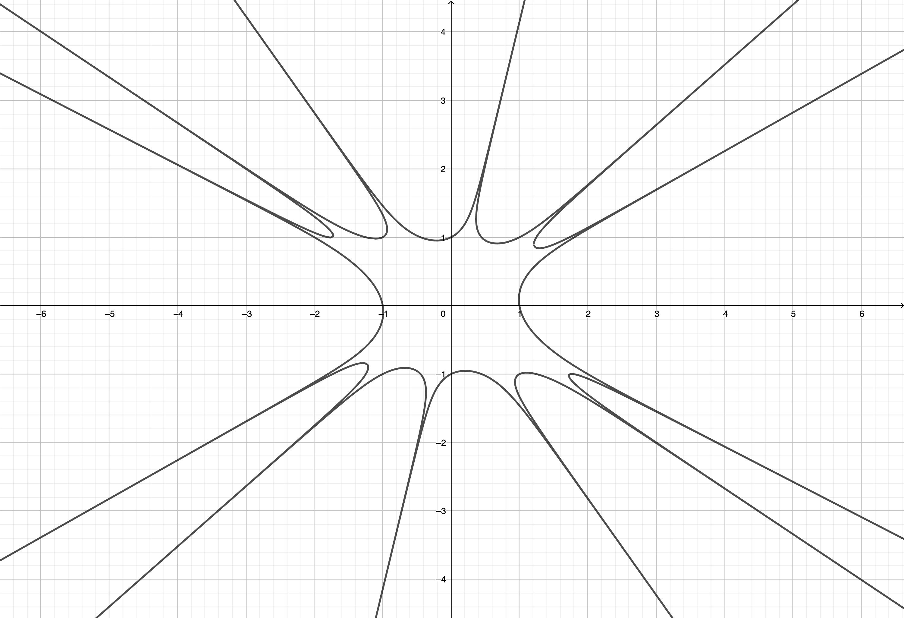
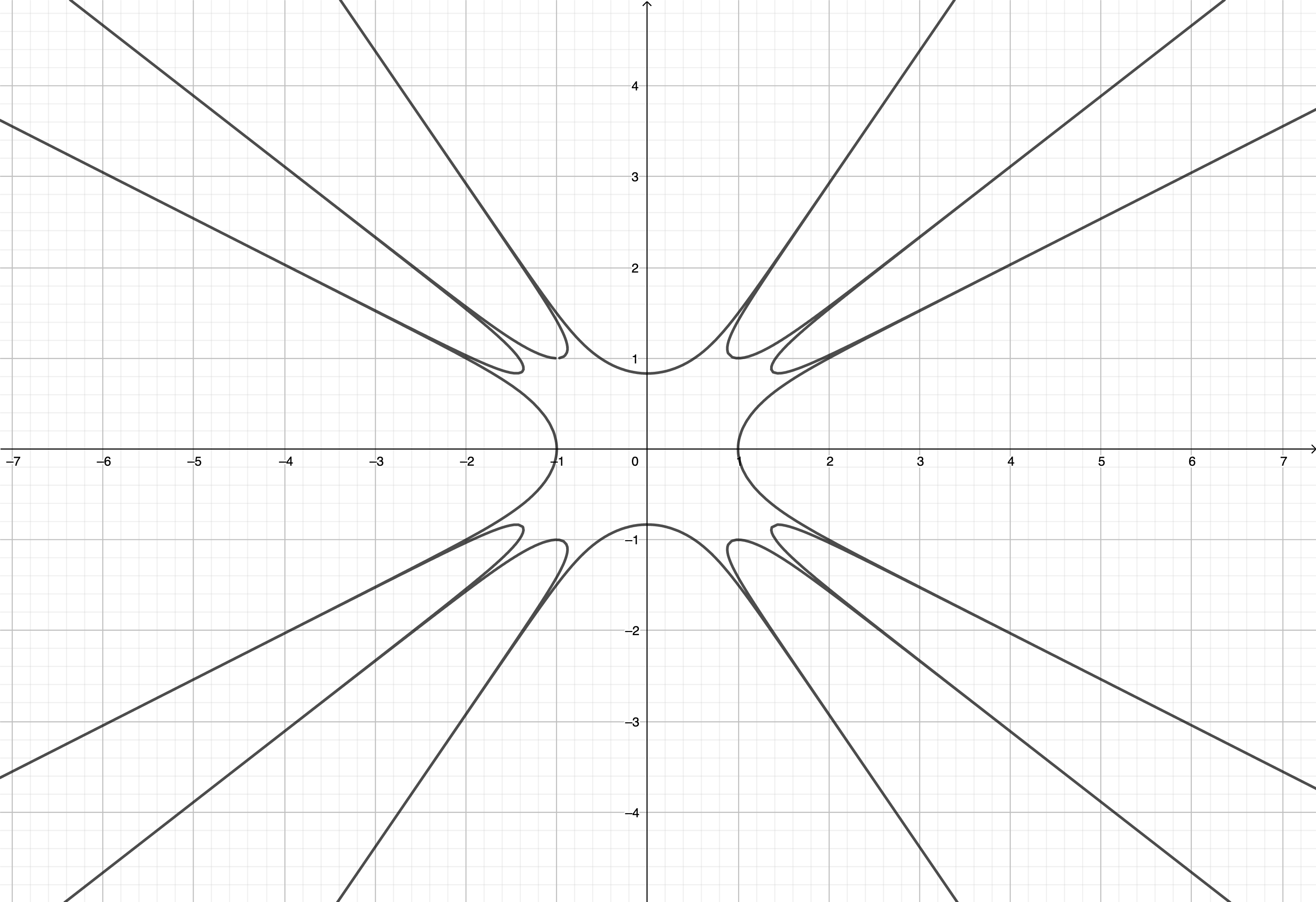
Figure 1: Graphs of $|\Psi_{13}(x,y)|=1$ (left) and $|\Pi_{9}(x,y)|=1$ (right)

Next, let $T_{n}(x)$ and $U_{n}(x)$ denote Chebyshev polynomials of the first and second kinds, respectively. The other two families that we are interested in are $T_{n}(x,y)$ and $U_{n}(x,y)$, which are homogenizations of $T_{n}(x)$ and $U_{n}(x)$, respectively. It is known [8] that

$$T_{n}(x,y)=2^{n-1}\prod\limits_{k=0}^{n-1}\left(x-\cos\left(\frac{(2k+1)\pi}{2n}\right)y\right)$$

and

$$U_{n}(x,y)=2^{n}\prod\limits_{k=1}^{n}\left(x-\cos\left(\frac{k\pi}{n+1}\right)y\right).$$

See Figure 2 for the graphs of $|T_{6}(x,y)|=1$ and $|U_{6}(x,y)|=1$. Note that in both cases the fundamental regions are not compact. It is also known that the binary forms $T_{n}(x,y)$ and $U_{n}(x,y)$ both have integer coefficients [8].

For a positive integer $n$, let $d(n)$ denote the number of its positive divisors. Let $\varphi(n)$ denote the Euler’s totient function. Our results are summarized in Theorem 1.1, Corollary 1.2, Theorem 1.3 and Theorem 1.4.

Theorem 1.1.

Let $n$ be a positive integer such that $\varphi(n)\geq 6$. Let $\Psi_{n}(x,y)$ denote the homogenization of the minimal polynomial of $2\cos\left(\frac{2\pi}{n}\right)$. Then

$$A_{\Psi_{n}} >\frac{16}{3}\exp\left(-\frac{2d(n)\log n}{\varphi(n)}\right)$$ (5)

$$A_{\Psi_{n}} <2^{\frac{4}{\varphi(n)}}\exp\left(\frac{2d(n)^{2}\log n}{\varphi(n)}\right)\times$$

$$\times\left[\frac{16}{3}+2^{1-\frac{4}{\varphi(n)}}B\left(\frac{1}{2},\frac{1}{2}-\frac{2}{\varphi(n)}\right)-2\pi+\left(\frac{2}{n}B\left(\frac{1}{n},1-\frac{4}{\varphi(n)}\right)-2\right)-\left(\frac{2}{n}B\left(\frac{3}{n},1-\frac{4}{\varphi(n)}\right)-\frac{2}{3}\right)\right].$$

Furthermore, $\lim\limits_{n\rightarrow\infty}A_{\Psi_{n}}=\frac{16}{3}$.

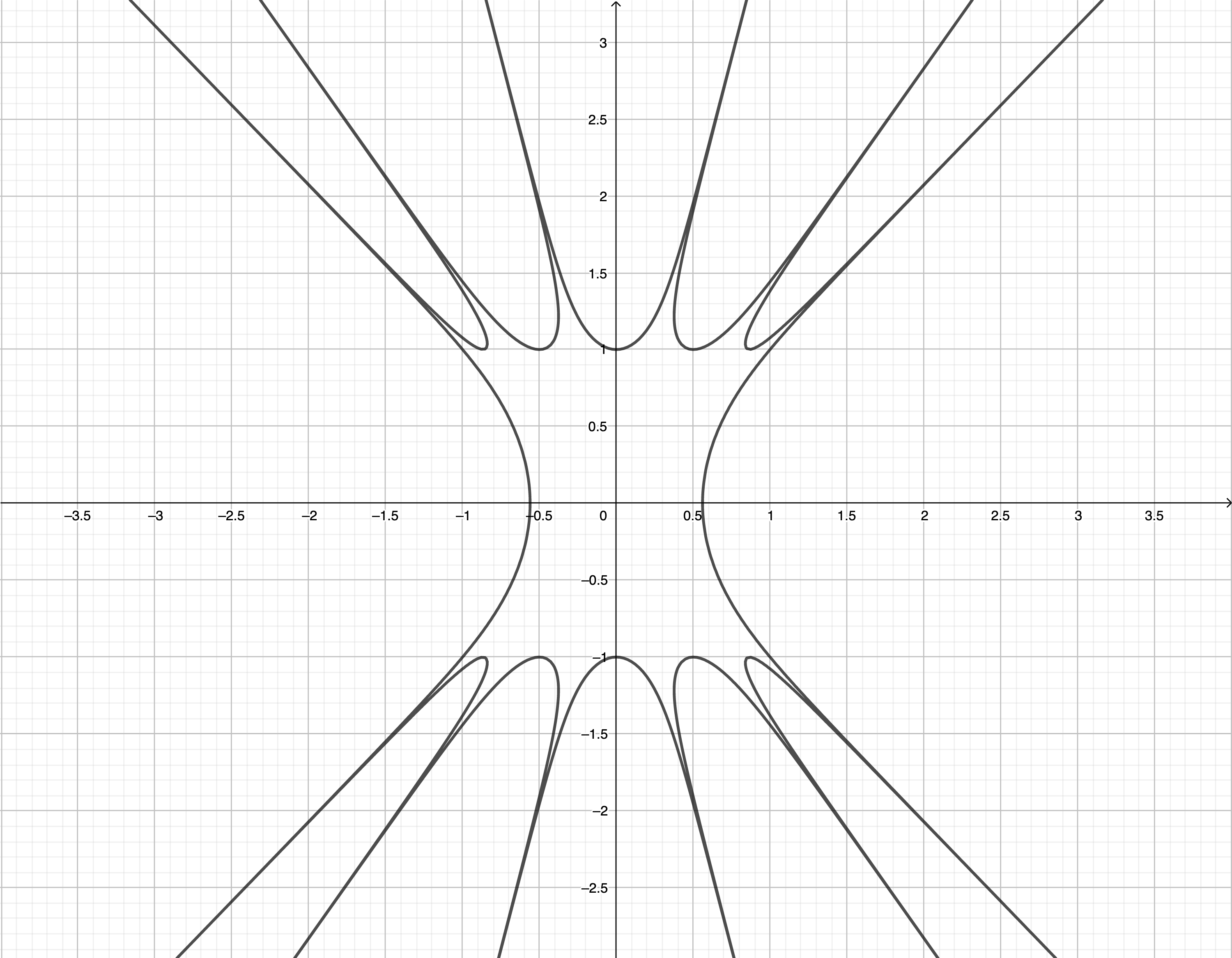
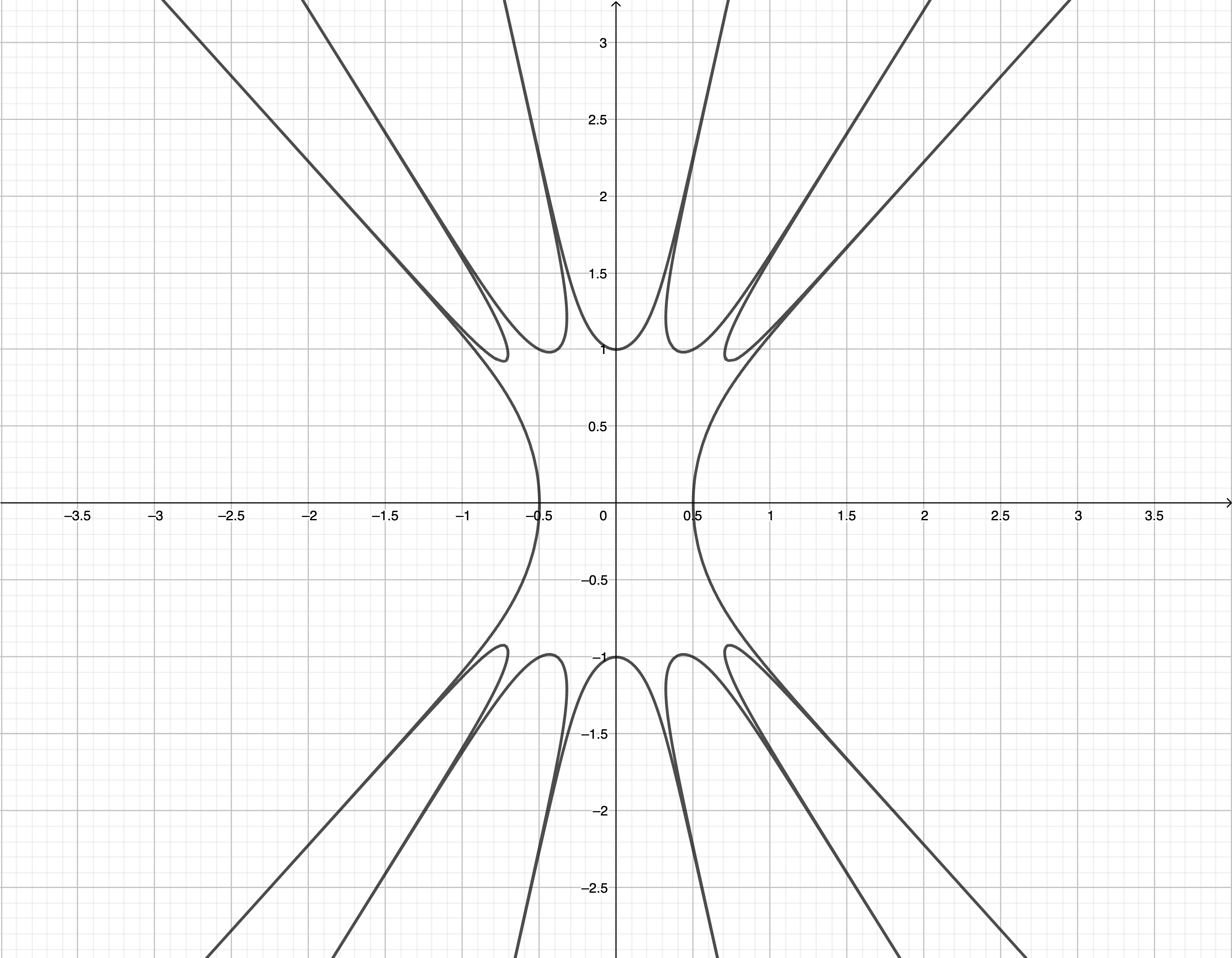
Figure 2: Graphs of $|T_{6}(x,y)|=1$ (left) and $|U_{6}(x,y)|=1$ (right)

Corollary 1.2.

Let $n$ be a positive integer. Let $\Pi_{n}(x,y)$ denote the homogenization of the minimal polynomial of $2\sin\left(\frac{2\pi}{n}\right)$. Then $\Pi_{n}(x,y)=\Psi_{c(n)}(x,y)$, where

$$c(n)=\begin{cases}4n&\text{if $n$ is odd,}\\ 2n&\text{if $n\equiv 2\pmod{4}$,}\\ n&\text{if $n\equiv 0\pmod{8}$,}\\ n/2&\text{if $n\equiv 12\pmod{16}$,}\\ n/4&\text{if $n\equiv 4\pmod{16}$.}\end{cases}$$

Furthermore, $\lim\limits_{n\rightarrow\infty}A_{\Pi_{n}}=\frac{16}{3}$.

Theorem 1.3.

Let $n$ be a positive integer such that $n\geq 3$. Let $T_{n}(x,y)$ denote the homogenization of the Chebyshev polynomial of the first kind $T_{n}(x)$. Then

$$\frac{8}{3}<A_{T_{n}}<\frac{8}{3}+\frac{2}{3}\left(\sqrt[n]{4}-1\right)+B\left(\frac{1}{2}-\frac{1}{n},\frac{1}{2}\right)-\pi$$ (6)

Furthermore, $\lim\limits_{n\rightarrow\infty}A_{T_{n}}=\frac{8}{3}$.

Theorem 1.4.

Let $n$ be a positive integer such that $n\geq 3$. Let $U_{n}(x,y)$ denote the homogenization of the Chebyshev polynomial of the second kind $U_{n}(x)$. Then

$$A_{U_{n}} >\frac{8}{3}+\left(B\left(1+\frac{1}{n},\frac{1}{2}\right)-2\right)+\frac{2}{3}\left((n+1)^{-2/n}-1\right)$$ (7)

$$A_{U_{n}} <\frac{8}{3}+\left(B\left(1+\frac{1}{n},\frac{1}{2}\right)-2\right)+B\left(\frac{1}{2}-\frac{1}{n},\frac{1}{2}\right)-\pi$$

Furthermore, $\lim\limits_{n\rightarrow\infty}A_{U_{n}}=\frac{8}{3}$.

Theorem 1.1 follows from Lemma 4.1, which we establish in Section 4. The proof of Corollary 1.2 is outlined in Section 5. Theorem 1.3 follows from Lemma 6.1, which we establish in Section 6. Theorem 1.4 follows from Lemma 7.1, which we establish in Section 7.

Our last result, which we present in Section 8, concerns the quantity

$$Q(F)=|D_{F}|^{1/n(n-1)}A_{F}$$

associated to a binary form $F$ of degree $n\geq 3$ and non-zero discriminant $D_{F}$. It was demonstrated by Bean [1] that the quantities $A_{F}$ and $Q(F)$ remain invariant for all binary forms that are equivalent under $\operatorname{GL}_{2}(\mathbb{Z})$ to $F$. Unlike $A_{F}$, the quantity $Q(F)$ also remains invariant for all binary forms that, up to multiplication by a complex number, are equivalent under $\operatorname{GL}_{2}(\mathbb{R})$ to $F$. An important conjecture about $Q(F)$ was formulated by Bean [2, Conjecture 1]. Let

$$F_{n}^{*}(x,y)=\prod\limits_{k=1}^{n}\left(\sin\left(\frac{k\pi}{n}\right)x-\cos\left(\frac{k\pi}{n}\right)y\right).$$

Conjecture 1.5.

The maximum value $M_{n}$ of $Q(F)$ over the forms $F$ with complex coefficients of degree $n$ with discriminant $D_{F}\neq 0$ is attained precisely when $F$ is a form which, up to multiplication by a complex number, is equivalent under $\operatorname{GL}_{2}(\mathbb{R})$ to the form $F_{n}^{*}$. That is, $M_{n}=Q(F_{n}^{*})$. Moreover, the limit of the sequence $\{M_{n}\}$ is $2\pi$.

It was proved by Bean and Laugesen [3, Theorem 1] that

$$Q(F_{n}^{*})=2^{1-2/n}n^{1/(n-1)}B\left(\frac{1}{2}-\frac{1}{n},\frac{1}{2}\right)$$ (8)

and that $\lim\limits_{n\rightarrow\infty}Q(F_{n}^{*})=2\pi$. Let $\nu_{2}(n)$ denote the $2$-adic order of $n$. In [9] it was proved by the author that the binary form

$$S_{n}(x,y)=2^{n-1-\nu_{2}(n)}F_{n}^{*}(x,y)$$

has integer coefficients and that the greatest common divisor of its coefficients is equal to one. See Figure 3 for the graph of $|S_{6}(x,y)|=1$. Just like the graph of $|F_{n}^{*}(x,y)|=1$, the graph of $|S_{n}(x,y)|=1$ is invariant under rotation by any integer multiple of $\frac{\pi}{n}$. In [9] it was also demonstrated that

$$A_{S_{n}}=4^{\nu_{2}(n)/n}B\left(\frac{1}{2}-\frac{1}{n},\frac{1}{2}\right),$$

and as a consequence that $\lim\limits_{n\rightarrow\infty}A_{S_{n}}=\pi$. Since $Q(F_{n}^{*})$ remains invariant under multiplication by a non-zero complex number, we see that $Q(S_{n})=Q(2^{n-1-\nu_{2}(n)}F_{n}^{*})=Q(F_{n}^{*})$. In Section 8 we will prove that $Q(T_{n})\leq Q(S_{n})$ and $Q(U_{n})\leq Q(S_{n})$ for every integer $n\geq 3$. We will also prove that

$$\lim\limits_{n\rightarrow\infty}Q(\Psi_{n})=\lim\limits_{n\rightarrow\infty}Q(\Pi_{n})=\lim\limits_{n\rightarrow\infty}Q(T_{n})=\lim\limits_{n\rightarrow\infty}Q(U_{n})=\frac{16}{3}.$$

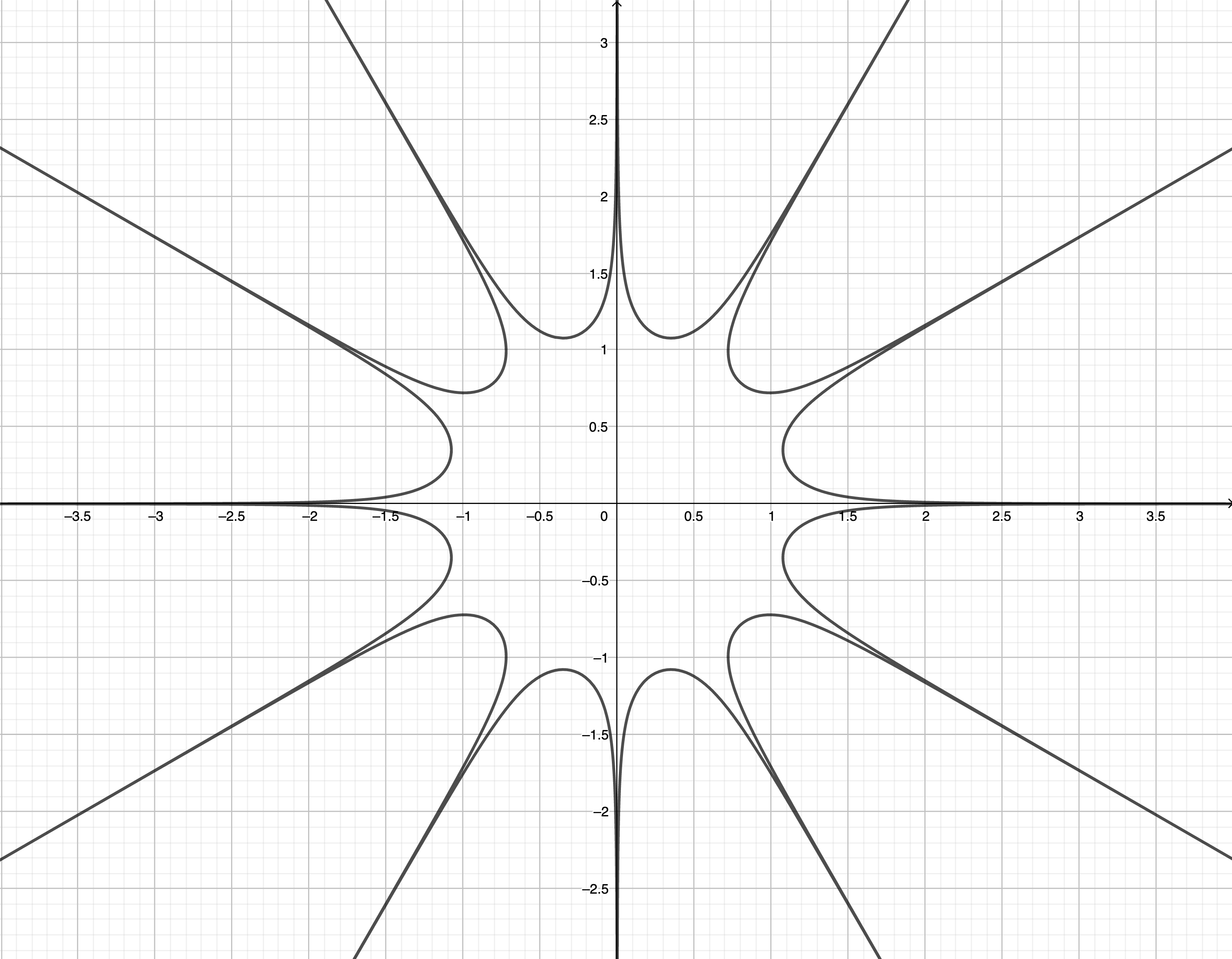
Figure 3: Graph of $|S_{6}(x,y)|=1$

$n$	$Q(\Psi_{n})$	$Q(\Pi_{n})$	$Q(S_{n})$	$Q(T_{n})$	$Q(U_{n})$
$3$	$\infty$	$\infty$	$15.8997$	$15.8997$	$15.8997$
$4$	$\infty$	$\infty$	$11.7726$	$11.4798$	$11.5438$
$5$	$\infty$	$10.8953$	$10.3228$	$9.85622$	$9.94897$
$6$	$\infty$	$\infty$	$9.55526$	$8.97702$	$9.08227$
$7$	$15.8997$	$8.5577$	$9.06881$	$8.41412$	$8.52393$
$8$	$\infty$	$\infty$	$8.72772$	$8.01814$	$8.12848$
$9$	$15.8997$	$9.00056$	$8.47265$	$7.72218$	$7.83097$

Table 1: Values of $Q(\Psi_{n})$, $Q(\Pi_{n})$, $Q(S_{n})$, $Q(T_{n})$ and $Q(U_{n})$ for $n=3,4,\ldots,9$.

2 Beta Function and Its Properties

For a complex number $z$ with positive real part, let

$$\Gamma(z)=\int\limits_{0}^{\infty}t^{z-1}e^{-t}dt$$ (9)

denote the gamma function. This function satisfies the functional equation

$$\Gamma(z+1)=z\Gamma(z).$$ (10)

The gamma function is analytic, with simple pole at $x=0$. Its residue at $x=0$ is equal to $1$, i.e.,

$$\operatorname{Res}(\Gamma(x),0)=\lim\limits_{x\rightarrow 0}x\Gamma(x)=1.$$ (11)

The beta function (2) can be expressed in terms of the gamma function by means of the relation

$$B(x,y)=\frac{\Gamma(x)\Gamma(y)}{\Gamma(x+y)}.$$ (12)

If in (2) we make the change of variables $t=\sin^{2}\theta$, then we obtain a trigonometric form of the beta function:

$$B(x,y)=2\int\limits_{0}^{\pi/2}(\sin\theta)^{2x-1}(\cos\theta)^{2y-1}d\theta.$$ (13)

This representation of $B(x,y)$ is used in the derivation of the formula for $A_{F_{n}^{*}}$ [9]. In Lemmas 4.1, 6.1 and 7.1 we will use it to obtain upper and lower bounds on $A_{\Psi_{n}}$, $A_{T_{n}}$ and $A_{U_{n}}$.

Finally, we would like to remark that the values of beta function can be easily computed numerically, as this function is present in various mathematical software, such as Maple (Beta(x, y)), Mathematica (Beta(x, y)) and MATLAB (beta(Z, W)).

3 The Limit of $A_{F_{n}}$ for $F_{n}(x,y)=ax^{n}+by^{n}$

In this section we prove the following result.

Proposition 3.1.

Let $a$, $b$ and $n$ be non-zero integers with $n\geq 3$ and let $F_{n}(x,y)=ax^{n}+by^{n}$. Then $\lim\limits_{n\rightarrow\infty}A_{F_{n}}=4$.

Proof.

In view of (3) and $\lim\limits_{n\rightarrow\infty}|ab|^{1/n}=1$, the result will follow once we show that

$$\lim\limits_{n\rightarrow\infty}\frac{1}{n}B\left(\frac{1}{n},1-\frac{2}{n}\right)=1\quad\text{and}\quad\lim\limits_{n\rightarrow\infty}\frac{1}{n}B\left(\frac{1}{n},\frac{1}{n}\right)=2.$$

To see that this is the case, first note that the identities

$$B\left(\frac{1}{n},1-\frac{2}{n}\right)=\frac{\Gamma(1/n)\Gamma(1-2/n)}{\Gamma(1-1/n)}\quad\text{and}\quad B\left(\frac{1}{n},\frac{1}{n}\right)=\frac{\Gamma(1/n)^{2}}{\Gamma(2/n)}$$

follow directly from (12). It follows from (11) that

$$\lim\limits_{n\rightarrow\infty}\frac{\Gamma(1/n)}{n}=1\quad\text{and}\quad\lim\limits_{n\rightarrow\infty}\frac{\Gamma(2/n)}{n}=\frac{1}{2}.$$

Since $\Gamma(1)=1$, we see that

$$\lim\limits_{n\rightarrow\infty}\frac{1}{n}B\left(\frac{1}{n},1-\frac{2}{n}\right)=\lim\limits_{n\rightarrow\infty}\frac{\Gamma(1/n)\Gamma(1-2/n)}{n\Gamma(1-1/n)}=\lim\limits_{n\rightarrow\infty}\frac{\Gamma(1/n)}{n}=1$$

and

$$\lim\limits_{n\rightarrow\infty}\frac{1}{n}B\left(\frac{1}{n},\frac{1}{n}\right)=\lim\limits_{n\rightarrow\infty}\frac{\Gamma(1/n)^{2}}{n\Gamma(2/n)}=\frac{\lim\limits_{n\rightarrow\infty}\left(\frac{\Gamma(1/n)}{n}\right)^{2}}{\lim\limits_{n\rightarrow\infty}\frac{\Gamma(2/n)}{n}}=2.$$

∎

4 Upper and Lower Bounds on $A_{\Psi_{n}}$

In this section we prove the following result.

Lemma 4.1.

For any $n\in\mathbb{N}$ and $\alpha\in\mathbb{R}$ such that $\varphi(n)\geq 4$ and $2/\varphi(n)<\alpha<1$,

$$\int\limits_{-\infty}^{+\infty}\frac{dx}{|\Psi_{n}(x)|^{\alpha}} >\left(4+\frac{16}{\varphi(n)^{2}\alpha^{2}-4}\right)\exp\left(-\frac{d(n)\log n}{2}\alpha\right)$$

$$\int\limits_{-\infty}^{+\infty}\frac{dx}{|\Psi_{n}(x)|^{\alpha}} <2^{\alpha}\exp\left(\frac{d(n)^{2}\log n}{2}\alpha\right),\times$$

$$\times\left[4+2^{1-\alpha}B\left(\frac{1-\alpha}{2},\frac{1}{2}\right)-2\pi+\frac{2}{n}B\left(\frac{\varphi(n)\alpha-2}{2n},1-\alpha\right)-\frac{2}{n}B\left(\frac{\varphi(n)\alpha+2}{2n},1-\alpha\right)\right].$$

Let us see why Theorem 1.1 directly follows from Lemma 4.1.

Proof of Theorem 1.1.

It follows from (4) that the degree of $\Psi_{n}$ is equal to $\varphi(n)/2$. Since the area $A_{\Psi_{n}}$ bounded by the curve $|\Psi_{n}(x,y)|=1$ can be computed via (1), the inequalities (5) follow from Lemma 4.1 once we take $\alpha=4/\varphi(n)$.

The fact that $\lim\limits_{n\rightarrow\infty}A_{\Psi_{n}}=\frac{16}{3}$ is a consequence of the following:

$$\lim\limits_{n\rightarrow\infty}B\left(\frac{1}{2},\frac{1}{2}-\frac{2}{\varphi(n)}\right)=B\left(\frac{1}{2},\frac{1}{2}\right)=\frac{\Gamma(1/2)^{2}}{\Gamma(1)}=\pi,$$

$$\lim\limits_{n\rightarrow\infty}\frac{2}{n}B\left(\frac{1}{n},1-\frac{4}{\varphi(n)}\right)=\lim\limits_{n\rightarrow\infty}\frac{2}{n}\Gamma\left(\frac{1}{n}\right)=2,$$

$$\lim\limits_{n\rightarrow\infty}\frac{2}{n}B\left(\frac{3}{n},1-\frac{4}{\varphi(n)}\right)=\lim\limits_{n\rightarrow\infty}\frac{2}{n}\Gamma\left(\frac{3}{n}\right)=\frac{2}{3}.$$

Further, we have

$$\lim\limits_{n\rightarrow\infty}\frac{2d(n)\log n}{\varphi(n)}=0\quad\text{and}\quad\lim\limits_{n\rightarrow\infty}\frac{2d(n)^{2}\log n}{\varphi(n)}=0.$$

These two limits follow from the fact that, for every integer $n>2$,

$$d(n)\leq n^{\frac{1.067}{\log\log n}}$$ (14)

and

$$\varphi(n)>\frac{n}{e^{\gamma}\log\log n+\frac{3}{\log\log n}}.$$ (15)

Here $\gamma\approx 0.5772$ denotes the Euler-Mascheroni constant. The upper bound on $d(n)$ was derived by Nicolas and Robin [10], while the lower bound on $\varphi(n)$ can be found in the paper of Rosser and Schoenfeld [12, Theorem 15]. ∎

Before proving Lemma 4.1, we need to establish three lemmas.

Lemma 4.2.

Let $n$ be an integer such that $n\geq 3$. Then, for every real number $\theta$,

$$\Psi_{n}(\pm 2\cos\theta)=(\pm 1)^{\frac{\varphi(n)}{2}}e^{-\frac{\varphi(n)}{2}\theta i}\Phi_{n}\left(\pm e^{\theta i}\right),$$ (16)

$$\Psi_{n}(\pm 2\cosh\theta)=(\pm 1)^{\frac{\varphi(n)}{2}}e^{\frac{\varphi(n)}{2}\theta}\Phi_{n}\left(\pm e^{-\theta}\right).$$ (17)

Proof.

According to Lehmer [5],

$$\Psi_{n}(x+x^{-1})=x^{-\varphi(n)/2}\Phi_{n}(x).$$

Putting $x=e^{\theta i}$, we obtain the identity (16), where the plus signs are chosen everywhere. Replacing $\theta$ with $\pi+\theta$, $\theta i$ and $\pi+\theta i$ we obtain the identity (16) where the minus signs are chosen everywhere, as well as the two identities in (17). ∎

For a polynomial $f(x)$, let $L(f)$ denote the sum of the absolute values of coefficients of $f(x)$. The following lemma can be found in [4, Lemme 4.1].

Lemma 4.3.

For every integer $n>1$, $L(\Phi_{n})\leq n^{\frac{d(n)}{2}}$.

Lemma 4.4.

For every positive integer $n$,

$$\prod\limits_{\begin{subarray}{c}m\mid n\\ m\neq 1\end{subarray}}L(\Phi_{m})\leq\exp\left(\frac{d(n)^{2}\log n}{2}\right).$$

Proof.

By Lemma 4.3,

$$\prod\limits_{\begin{subarray}{c}m\mid n\\ m\neq 1\end{subarray}}L(\Phi_{m}) \leq\prod\limits_{m\mid n}m^{\frac{d(m)}{2}}$$

$$=\exp\left(\frac{1}{2}\sum\limits_{m\mid n}d(m)\log m\right)$$

$$\leq\exp\left(\frac{d(n)\log n}{2}\sum\limits_{m\mid n}1\right)$$

$$=\exp\left(\frac{d(n)^{2}\log n}{2}\right).$$

∎

Proof of Lemma 4.1.

Note that

$$\int\limits_{-\infty}^{+\infty}\frac{dx}{|\Psi_{n}(x)|^{\alpha}} =\int\limits_{-2}^{2}\frac{dx}{|\Psi_{n}(x)|^{\alpha}}+\int\limits_{2}^{+\infty}\frac{dx}{|\Psi_{n}(x)|^{\alpha}}+\int\limits_{-\infty}^{-2}\frac{dx}{|\Psi_{n}(x)|^{\alpha}}$$

$$=-\int\limits_{0}^{\pi}\frac{d(2\cos\theta)}{|\Psi_{n}(2\cos\theta)|^{\alpha}}+\int\limits_{0}^{+\infty}\frac{d(2\cosh\theta)}{|\Psi_{n}(2\cosh\theta)|^{\alpha}}+\int\limits_{-\infty}^{0}\frac{d(-2\cosh\theta)}{|\Psi_{n}(-2\cosh\theta)|^{\alpha}}$$

$$=2\int\limits_{0}^{\pi}\frac{\sin\theta d\theta}{|\Psi_{n}(2\cos\theta)|^{\alpha}}+2\int\limits_{0}^{+\infty}\frac{\sinh\theta d\theta}{|\Psi_{n}(2\cosh\theta)|^{\alpha}}+2\int\limits_{0}^{+\infty}\frac{\sinh\theta d\theta}{|\Psi_{n}(-2\cosh\theta)|^{\alpha}}$$

$$=2\int\limits_{0}^{\pi}\frac{\sin\theta d\theta}{|\Phi_{n}(e^{\theta i})|^{\alpha}}+2\int\limits_{0}^{+\infty}\frac{\sinh\theta d\theta}{e^{(\varphi(n)/2)\alpha\theta}\Phi_{n}(e^{-\theta})^{\alpha}}+2\int\limits_{0}^{+\infty}\frac{\sinh\theta d\theta}{e^{(\varphi(n)/2)\alpha\theta}\Phi_{n}(-e^{-\theta})^{\alpha}},$$

where the last equality follows from Lemma 4.2. Let

$$C_{1}=2\int\limits_{0}^{\pi}\frac{\sin\theta d\theta}{|\Phi_{n}(e^{\theta i})|^{\alpha}},\quad C_{2}=2\int\limits_{0}^{+\infty}\frac{\sinh\theta d\theta}{e^{(\varphi(n)/2)\alpha\theta}\Phi_{n}(e^{-\theta})^{\alpha}},\quad C_{3}=2\int\limits_{0}^{+\infty}\frac{\sinh\theta d\theta}{e^{(\varphi(n)/2)\alpha\theta}\Phi_{n}(-e^{-\theta})^{\alpha}}.$$

We will now derive upper and lower bounds on $C_{1}$, $C_{2}$ and $C_{3}$.

We begin with the derivation of a lower bound. By Lemma 4.3,

$$|\Phi_{n}(z)|\leq L(\Phi_{n})\max\{1,|z|\}^{\varphi(n)}\leq n^{\frac{d(n)}{2}}$$

for all $z\in\mathbb{C}$ such that $|z|\leq 1$. In view of this,

$$C_{1} =2\int\limits_{0}^{\pi}\frac{\sin\theta d\theta}{|\Phi_{n}(e^{\theta i})|^{\alpha}}$$

$$\geq 2n^{-\frac{d(n)}{2}\alpha}\int\limits_{0}^{\pi}\sin\theta d\theta$$

$$=4\exp\left(-\frac{d(n)\log n}{2}\alpha\right)$$

and

$$C_{2} =2\int\limits_{0}^{+\infty}\frac{\sinh\theta d\theta}{e^{(\varphi(n)/2)\alpha\theta}\Phi_{n}\left(e^{-\theta}\right)^{\alpha}}$$

$$\geq 2n^{-\frac{d(n)}{2}\alpha}\int\limits_{0}^{+\infty}e^{-\frac{\varphi(n)}{2}\alpha\theta}\sinh\theta d\theta$$

$$=2n^{-\frac{d(n)}{2}\alpha}\frac{1}{\left(\frac{\varphi(n)}{2}\alpha\right)^{2}-1}$$

$$=\frac{8}{\varphi(n)^{2}\alpha^{2}-4}\exp\left(-\frac{d(n)\log n}{2}\alpha\right).$$

Similarly,

$$C_{3}\geq\frac{8}{\varphi(n)^{2}\alpha^{2}-4}\exp\left(-\frac{d(n)\log n}{2}\alpha\right).$$

We conclude that

$$\int\limits_{-\infty}^{+\infty}\frac{dx}{|\Psi_{n}(x)|^{\alpha}}=C_{1}+C_{2}+C_{3}\geq\left(4+\frac{16}{\varphi(n)^{2}\alpha^{2}-4}\right)\exp\left(-\frac{d(n)\log n}{2}\alpha\right).$$

To derive an upper bound, we will make use of the identity

$$z^{n}-1=\prod\limits_{m\mid n}\Phi_{m}(z).$$

Notice that

$$\Phi_{n}(z)=(z^{n}-1)\prod\limits_{\begin{subarray}{c}m\mid n\\ m\neq n\end{subarray}}\Phi_{m}(z)^{-1}.$$

Thus for every $z\in\mathbb{C}$ such that $|z|<1$ we have

$$|\Phi_{n}(z)|^{-1} =\frac{1}{|z^{n}-1|}\prod\limits_{\begin{subarray}{c}m\mid n\\ m\neq n\end{subarray}}|\Phi_{m}(z)|$$

$$=\frac{|z-1|}{|z^{n}-1|}\prod\limits_{\begin{subarray}{c}m\mid n\\ 1<m<n\end{subarray}}|\Phi_{m}(z)|$$

$$\leq\frac{|z-1|}{|z^{n}-1|}\prod\limits_{\begin{subarray}{c}m\mid n\\ m\neq 1\end{subarray}}L(\Phi_{m})$$

$$<\frac{2}{|z^{n}-1|}\exp\left(\frac{d(n)^{2}\log n}{2}\right),$$

where the last inequality follows from Lemma 4.4. In view of this,

$$C_{1} =2\int\limits_{0}^{\pi}\frac{\sin\theta d\theta}{|\Phi_{n}(e^{\theta i})|^{\alpha}}$$

$$\leq 2^{1+\alpha}\exp\left(\frac{d(n)^{2}\log n}{2}\alpha\right)\int\limits_{0}^{\pi}\frac{\sin\theta d\theta}{|e^{n\theta i}-1|^{\alpha}}$$

$$=2^{1+\alpha}\exp\left(\frac{d(n)^{2}\log n}{2}\alpha\right)\left(\int\limits_{0}^{\pi}\sin\theta d\theta+\int\limits_{0}^{\pi}\sin\theta\left(|e^{n\theta i}-1|^{-\alpha}-1\right)d\theta\right)$$

$$\leq 2^{1+\alpha}\exp\left(\frac{d(n)^{2}\log n}{2}\alpha\right)\left(2+\int\limits_{0}^{\pi}\left(\frac{1}{|e^{n\theta i}-1|^{\alpha}}-1\right)d\theta\right)$$

$$=2^{1+\alpha}\exp\left(\frac{d(n)^{2}\log n}{2}\alpha\right)\left(2+\int\limits_{0}^{\pi}\frac{d\theta}{|e^{n\theta i}-1|^{\alpha}}-\pi\right).$$

It remains to estimate the integral $\int_{0}^{\pi}\frac{d\theta}{|e^{n\theta i}-1|^{\alpha}}$. Note that

$$|e^{n\theta i}-1|^{2}=\left(\cos(n\theta)-1\right)^{2}+\sin^{2}(n\theta)=2-2\cos(n\theta)=4\sin^{2}\left(\frac{n\theta}{2}\right).$$

Therefore,

$$\int_{0}^{\pi}\frac{d\theta}{|e^{n\theta i}-1|^{\alpha}} =2^{-\alpha}\int\limits_{0}^{\pi}\left|\sin\left(\frac{n\theta}{2}\right)\right|^{-\alpha}d\theta$$

$$=\frac{2^{1-\alpha}}{n}\int\limits_{0}^{n\pi/2}\left|\sin\theta\right|^{-\alpha}d\theta$$

$$=2^{-\alpha}\cdot 2\int\limits_{0}^{\pi/2}\left(\sin\theta\right)^{-\alpha}d\theta$$

$$=2^{-\alpha}B\left(\frac{1-\alpha}{2},\frac{1}{2}\right).$$

We conclude that

$$C_{1} =2\int\limits_{0}^{\pi}\frac{\sin\theta d\theta}{|\Phi_{n}(e^{\theta i})|^{\alpha}}$$

$$\leq 2^{\alpha}\exp\left(\frac{d(n)^{2}\log n}{2}\alpha\right)\left(4+2^{1-\alpha}B\left(\frac{1-\alpha}{2},\frac{1}{2}\right)-2\pi\right).$$

Next, we derive an upper bound on $C_{2}$:

$$C_{2} =2\int\limits_{0}^{+\infty}\frac{\sinh\theta d\theta}{e^{(\varphi(n)/2)\alpha\theta}\Phi_{n}(e^{-\theta})^{\alpha}}$$

$$\leq 2^{1+\alpha}\exp\left(\frac{d(n)^{2}\log n}{2}\alpha\right)\int\limits_{0}^{+\infty}\frac{\sinh\theta d\theta}{e^{(\varphi(n)/2)\alpha\theta}(1-e^{-n\theta})^{\alpha}}$$

$$=2^{1+\alpha}\exp\left(\frac{d(n)^{2}\log n}{2}\alpha\right)\frac{1}{2n}\int\limits_{0}^{1}\left(t^{\frac{\varphi(n)\alpha-2}{2n}-1}-t^{\frac{\varphi(n)\alpha+2}{2n}-1}\right)(1-t)^{-\alpha}dt$$

$$=2^{\alpha}\exp\left(\frac{d(n)^{2}\log n}{2}\alpha\right)\left(\frac{1}{n}B\left(\frac{\varphi(n)\alpha-2}{2n},1-\alpha\right)-\frac{1}{n}B\left(\frac{\varphi(n)\alpha+2}{2n},1-\alpha\right)\right),$$

where the second-to-last equality follows from the change of variables $t=e^{-n\theta}$.

Finally, we derive an upper bound on $C_{3}$. We consider two cases.

Case 1. Suppose that $n$ is even. Then

$$C_{3} =2\int\limits_{0}^{+\infty}\frac{\sinh\theta d\theta}{e^{(\varphi(n)/2)\alpha\theta}\Phi_{n}(-e^{-\theta})^{\alpha}}$$

$$\leq 2^{1+\alpha}\exp\left(\frac{d(n)^{2}\log n}{2}\alpha\right)\int\limits_{0}^{+\infty}\frac{\sinh\theta d\theta}{e^{(\varphi(n)/2)\alpha\theta}\left(1-(-e^{-\theta})^{n}\right)^{\alpha}}$$

$$=2^{1+\alpha}\exp\left(\frac{d(n)^{2}\log n}{2}\alpha\right)\int\limits_{0}^{+\infty}\frac{\sinh\theta d\theta}{e^{(\varphi(n)/2)\alpha\theta}\left(1-e^{-n\theta}\right)^{\alpha}}$$

$$=2^{\alpha}\exp\left(\frac{d(n)^{2}\log n}{2}\alpha\right)\left(\frac{1}{n}B\left(\frac{\varphi(n)\alpha-2}{2n},1-\alpha\right)-\frac{1}{n}B\left(\frac{\varphi(n)\alpha+2}{2n},1-\alpha\right)\right),$$

where the last equality was derived from the estimate for $C_{2}$.

Case 2. Suppose that $n$ is odd. Then for any real number $x$ we have $\Phi_{n}(-x)=\Phi_{2n}(x)$, so

$$C_{3} =2\int\limits_{0}^{+\infty}\frac{\sinh\theta d\theta}{e^{(\varphi(n)/2)\alpha\theta}\Phi_{n}(-e^{-\theta})^{\alpha}}$$

$$=2\int\limits_{0}^{+\infty}\frac{\sinh\theta d\theta}{e^{(\varphi(n)/2)\alpha\theta}\Phi_{2n}(e^{-\theta})^{\alpha}}$$

$$\leq 2^{1+\alpha}\exp\left(\frac{d(n)^{2}\log n}{2}\alpha\right)\int\limits_{0}^{+\infty}\frac{\sinh\theta d\theta}{e^{(\varphi(n)/2)\alpha\theta}\left(1-e^{-2n\theta}\right)^{\alpha}}$$

$$\leq 2^{1+\alpha}\exp\left(\frac{d(n)^{2}\log n}{2}\alpha\right)\int\limits_{0}^{+\infty}\frac{\sinh\theta d\theta}{e^{(\varphi(n)/2)\alpha\theta}\left(1-e^{-n\theta}\right)^{\alpha}}$$

$$=2^{\alpha}\exp\left(\frac{d(n)^{2}\log n}{2}\alpha\right)\left(\frac{1}{n}B\left(\frac{\varphi(n)\alpha-2}{2n},1-\alpha\right)-\frac{1}{n}B\left(\frac{\varphi(n)\alpha+2}{2n},1-\alpha\right)\right),$$

where the last equality was derived from the estimate for $C_{2}$.

We conclude that

$$\int\limits_{-\infty}^{+\infty}\frac{dx}{|\Psi_{n}(x)|^{\alpha}} =C_{1}+C_{2}+C_{3}$$

$$\leq 2^{\alpha}\exp\left(\frac{d(n)^{2}\log n}{2}\alpha\right)\times$$

$$\times\left(4+2^{1-\alpha}B\left(\frac{1-\alpha}{2},\frac{1}{2}\right)-2\pi+\frac{2}{n}B\left(\frac{\varphi(n)\alpha-2}{2n},1-\alpha\right)-\frac{2}{n}B\left(\frac{\varphi(n)\alpha+2}{2n},1-\alpha\right)\right).$$

∎

5 Proof of Corollary 1.2

In view of the identity $\sin\left(\frac{2\pi}{n}\right)=\cos\left(\frac{2\pi(n-4)}{4n}\right)$, we can follow the argument of Niven [11, III.4] and consider the following five cases.

1. If $n$ is odd, then the fraction $\frac{n-4}{4n}$ is in lowest terms. Thus $2\cos\left(\frac{2\pi(n-4)}{4n}\right)$ is conjugate to $2\cos\left(\frac{2\pi}{4n}\right)$ and $c(n)=4n$.

2. If $n\equiv 2\pmod{4}$, then $\frac{n-4}{4n}$ reduces to a fraction with denominator $2n$. Thus $2\cos\left(\frac{2\pi(n-4)}{4n}\right)$ is conjugate to $2\cos\left(\frac{2\pi}{2n}\right)$ and $c(n)=2n$.

3. If $n\equiv 0\pmod{8}$, then $\frac{n-4}{4n}$ reduces to a fraction with denominator $n$. Thus $2\cos\left(\frac{2\pi(n-4)}{4n}\right)$ is conjugate to $2\cos\left(\frac{2\pi}{n}\right)$ and $c(n)=n$.

4. If $n\equiv 12\pmod{16}$, then $\frac{n-4}{4n}$ reduces to a fraction with denominator $n/2$. Thus $2\cos\left(\frac{2\pi(n-4)}{4n}\right)$ is conjugate to $2\cos\left(\frac{2\pi}{n/2}\right)$ and $c(n)=n/2$.

5. If $n\equiv 4\pmod{16}$, then $\frac{n-4}{4n}$ reduces to a fraction with denominator $n/4$. Thus $2\cos\left(\frac{2\pi(n-4)}{4n}\right)$ is conjugate to $2\cos\left(\frac{2\pi}{n/4}\right)$ and $c(n)=n/4$.

A combination of this result with Theorem 1.1 yields $\lim\limits_{n\rightarrow\infty}A_{\Pi_{n}}=\lim\limits_{n\rightarrow\infty}A_{\Psi_{n}}=\frac{16}{3}$.

6 Upper and Lower Bounds on $A_{T_{n}}$

In this section we prove the following result.

Lemma 6.1.

For any $n\in\mathbb{N}$ and $\alpha\in\mathbb{R}$ such that $n\geq 3$ and $2/n\leq\alpha<1$,

$$2+\frac{2}{n^{2}\alpha^{2}-1}<\int_{-\infty}^{+\infty}\frac{dx}{|T_{n}(x)|^{\alpha}}<2+\frac{2^{1+\alpha}}{n^{2}\alpha^{2}-1}+B\left(\frac{1-\alpha}{2},\frac{1}{2}\right)-\pi.$$

Let us see why Theorem 1.3 directly follows from Lemma 6.1.

Proof of Theorem 1.3.

Since for an arbitrary binary form $F$ of positive degree $n$ the area bounded by the curve $|F(x,y)|=1$ can be computed via (1), the inequalities (6) follow from Lemma 6.1 if we take $\alpha=2/n$.

To see that $\lim\limits_{n\rightarrow\infty}A_{T_{n}}=\frac{8}{3}$, it is sufficient to demonstrate that the limit of $B\left(\frac{1}{2}-\frac{1}{n},\frac{1}{2}\right)$ as $n$ approaches infinity is equal to $\pi$. Recall that the gamma function (9) satisfies $\Gamma(1)=1$ and $\Gamma(1/2)=\sqrt{\pi}$. In view of (12), we see that

$$\lim\limits_{n\rightarrow\infty}B\left(\frac{1}{2}-\frac{1}{n},\frac{1}{2}\right)=B\left(\frac{1}{2},\frac{1}{2}\right)=\frac{\Gamma(1/2)^{2}}{\Gamma(1)}=\pi.$$

∎

We will now turn our attention to the proof of Lemma 6.1.

Proof of Lemma 6.1.

Since the function $|T_{n}(x)|$ is even, we find that

$$\int_{-\infty}^{+\infty}\frac{dx}{|T_{n}(x)|^{\alpha}}=C_{1}+C_{2},$$

where

$$C_{1}=2\int\limits_{1}^{+\infty}\frac{dx}{T_{n}(x)^{\alpha}},\,\,\,C_{2}=2\int\limits_{0}^{1}\frac{dx}{|T_{n}(x)|^{\alpha}},$$

We will now derive upper and lower bounds on $C_{1}$ and $C_{2}$.

First, we determine upper and lower bounds on $C_{1}$. Recall that

$$T_{n}(x)=\frac{(x+\sqrt{x^{2}-1})^{n}+(x-\sqrt{x^{2}-1})^{n}}{2}$$

for all $x$ such that $|x|\geq 1$. Hence

$$\frac{(x+\sqrt{x^{2}-1})^{n}}{2}<T_{n}(x)<(x+\sqrt{x^{2}-1})^{n}$$ (18)

for all $x>1$. Using the lower bound in (18), as well as the change of variables $x=\csc\theta$, we find that

$$C_{1} =2\int\limits_{1}^{+\infty}\frac{dx}{T_{n}(x)^{\alpha}}$$

$$<2^{\alpha+1}\int\limits_{1}^{+\infty}\frac{dx}{(x+\sqrt{x^{2}-1})^{n\alpha}}$$

$$=2^{\alpha+1}\int\limits_{0}^{\pi/2}\frac{(\cos\theta)(\sin\theta)^{n\alpha-2}d\theta}{(1+\cos\theta)^{n\alpha}}$$

$$=2^{\alpha+1}\left.\frac{(\sin\theta)^{n\alpha-1}(n\alpha\cos\theta+1)}{(n^{2}\alpha^{2}-1)(1+\cos\theta)^{n\alpha}}\right|_{0}^{\pi/2}$$

$$=\frac{2^{\alpha+1}}{n^{2}\alpha^{2}-1}$$

A lower bound on $C_{1}$ can be obtained analogously. As a result, we get

$$\frac{2}{n^{2}\alpha^{2}-1}<C_{1}<\frac{2^{1+\alpha}}{n^{2}\alpha^{2}-1}.$$

Next, we determine upper and lower bounds on $C_{2}$. We apply the substitution $x=\cos(\theta/n)$ and make use of the identity $\cos\theta=T_{n}(\cos(\theta/n))$ as follows:

$$C_{2} =2\int\limits_{0}^{1}\frac{dx}{|T_{n}(x)|^{\alpha}}$$

$$=\frac{2}{n}\int\limits_{0}^{\pi n/2}\frac{\sin(\theta/n)d\theta}{|\cos\theta|^{\alpha}}$$

$$=\frac{2}{n}\int\limits_{0}^{\pi n/2}\sin(\theta/n)d\theta+\varepsilon_{n},$$

where

$$\varepsilon_{n}=\frac{2}{n}\int\limits_{0}^{\pi n/2}\sin(\theta/n)\left(|\cos\theta|^{-\alpha}-1\right)d\theta.$$

Note that $\varepsilon_{n}>0$. Since

$$\frac{2}{n}\int\limits_{0}^{\pi n/2}\sin(\theta/n)d\theta=2\int\limits_{0}^{\pi/2}\sin\theta d\theta=2,$$

we have

$$C_{2}=\frac{2}{n}\int\limits_{0}^{\pi n/2}\sin(\theta/n)d\theta+\varepsilon_{n}>2.$$

It remains to find an upper bound on $C_{2}$. Note that

$$\varepsilon_{n} =\frac{2}{n}\int\limits_{0}^{\pi n/2}\sin(\theta/n)\left(|\cos\theta|^{-\alpha}-1\right)d\theta$$

$$\leq\frac{2}{n}\int\limits_{0}^{\pi n/2}|\cos\theta|^{-\alpha}d\theta-\pi$$

$$=2\int\limits_{0}^{\pi/2}(\cos\theta)^{-\alpha}d\theta-\pi$$

$$=B\left(\frac{1-\alpha}{2},\frac{1}{2}\right)-\pi,$$

where the last equality follows from (13). We conclude that

$$2<C_{2}\leq 2+B\left(\frac{1-\alpha}{2},\frac{1}{2}\right)-\pi.$$

∎

7 Upper and Lower Bounds on $A_{U_{n}}$

In this section we prove the following result.

Lemma 7.1.

For any $n\in\mathbb{N}$ and $\alpha\in\mathbb{R}$ such that $n\geq 3$ and $2/n\leq\alpha<1$,

$$\int\limits_{-\infty}^{+\infty}\frac{dx}{|U_{n}(x)|^{\alpha}} >B\left(\frac{2+\alpha}{2},\frac{1}{2}\right)+\frac{2}{n^{2}\alpha^{2}-1}(n+1)^{-\alpha}$$

$$\int\limits_{-\infty}^{+\infty}\frac{dx}{|U_{n}(x)|^{\alpha}} <B\left(\frac{2+\alpha}{2},\frac{1}{2}\right)+\frac{2}{n^{2}\alpha^{2}-1}+B\left(\frac{1-\alpha}{2},\frac{1}{2}\right)-\pi$$

Let us see why Theorem 1.4 directly follows from Lemma 7.1.

Proof of Theorem 1.4.

Since for an arbitrary binary form $F$ of positive degree $n$ the area bounded by the curve $|F(x,y)|=1$ can be computed via (1), the inequalities (7) follow from Lemma 7.1 if we take $\alpha=2/n$.

To see that $\lim\limits_{n\rightarrow\infty}A_{U_{n}}=\frac{8}{3}$, it is sufficient to demonstrate that the limits of $B\left(\frac{1}{2}-\frac{1}{n},\frac{1}{2}\right)$ and $B\left(1+\frac{1}{n},\frac{1}{2}\right)$ as $n$ approaches infinity are equal to $\pi$ and $2$, respectively. Recall that the gamma function (9) satisfies $\Gamma(1)=1$ and $\Gamma(1/2)=\sqrt{\pi}$. In view of (12), we see that

$$\lim\limits_{n\rightarrow\infty}B\left(\frac{1}{2}-\frac{1}{n},\frac{1}{2}\right)=B\left(\frac{1}{2},\frac{1}{2}\right)=\frac{\Gamma(1/2)^{2}}{\Gamma(1)}=\pi$$

and

$$\lim\limits_{n\rightarrow\infty}B\left(1+\frac{1}{n},\frac{1}{2}\right)=B\left(1,\frac{1}{2}\right)=\frac{\Gamma(1)\Gamma(1/2)}{\Gamma(3/2)}=\frac{\Gamma(1)\Gamma(1/2)}{(1/2)\Gamma(1/2)}=2,$$

where the second-to-last equality follows from the functional equation (10). ∎

We will now turn our attention to the proof of Lemma 7.1.

Proof of Lemma 7.1.

Since the function $|U_{n}(x)|$ is even, we find that

$$\int_{-\infty}^{+\infty}\frac{dx}{|U_{n}(x)|^{\alpha}}=C_{1}+C_{2},$$

where

$$C_{1}=2\int\limits_{1}^{+\infty}\frac{dx}{U_{n}(x)^{\alpha}},\,\,\,C_{2}=2\int\limits_{0}^{1}\frac{dx}{|U_{n}(x)|^{\alpha}}.$$

We will now derive upper and lower bounds on $C_{1}$ and $C_{2}$.

Put $C_{1}=2\int\limits_{1}^{+\infty}\frac{dx}{U_{n}(x)^{\alpha}},\,\,\,C_{2}=2\int\limits_{0}^{1}\frac{dx}{|U_{n}(x)|^{\alpha}}$, so that $\int\limits_{-\infty}^{+\infty}\frac{dx}{|U_{n}(x)|^{\alpha}}=C_{1}+C_{2}$.

First, we determine upper and lower bounds on $C_{1}$. Recall that

$$U_{n}(x)=\frac{\left(x+\sqrt{x^{2}-1}\right)^{n+1}-\left(x-\sqrt{x^{2}-1}\right)^{n+1}}{2\sqrt{x^{2}-1}}$$

for all $x$ such that $|x|\geq 1$. Thus for every $\theta\in[0,\pi/2]$ we have

$$(\sin\theta)^{n}U_{n}(\csc\theta) =\frac{(1+\cos\theta)^{n+1}-(1-\cos\theta)^{n+1}}{2\cos\theta}$$

$$=\frac{\left(2\cos^{2}\frac{\theta}{2}\right)^{n+1}-\left(2\sin^{2}\frac{\theta}{2}\right)^{n+1}}{2\cos\theta}$$

$$=2^{n}\sum\limits_{k=0}^{n}\left(\sin^{2}\frac{\theta}{2}\right)^{k}\left(\cos^{2}\frac{\theta}{2}\right)^{n-k}.$$

Since

$$\left(\cos^{2}\frac{\theta}{2}\right)^{n}<\sum\limits_{k=0}^{n}\left(\sin^{2}\frac{\theta}{2}\right)^{k}\left(\cos^{2}\frac{\theta}{2}\right)^{n-k}<(n+1)\left(\cos^{2}\frac{\theta}{2}\right)^{n}$$

for every $\theta\in(0,\pi/2]$, we find that

$$\left(1+\cos\theta\right)^{n}<(\sin\theta)^{n}U_{n}(\csc\theta)<(n+1)\left(1+\cos\theta\right)^{n}$$ (19)

for every $\theta\in(0,\pi/2]$.

Using the change of variables $x=\csc\theta$, as well as the lower bound in (19), we find that

$$C_{1} =2\int\limits_{1}^{+\infty}\frac{dx}{U_{n}(x)^{\alpha}}$$

$$=2\int\limits_{0}^{\pi/2}\frac{\cos\theta d\theta}{(\sin\theta)^{2}U_{n}(\csc\theta)^{\alpha}}$$

$$<2\int\limits_{0}^{\pi/2}\frac{\cos\theta(\sin\theta)^{n\alpha-2}d\theta}{(1+\cos\theta)^{n\alpha}}$$

$$=2\left.\frac{(\sin\theta)^{n\alpha-1}(n\alpha\cos\theta+1)}{(n^{2}\alpha^{2}-1)(1+\cos\theta)^{n\alpha}}\right|_{0}^{\pi/2}$$

$$=\frac{2}{n^{2}\alpha^{2}-1}.$$

A lower bound on $C_{1}$ can be obtained analogously. As a result, we get

$$\frac{2}{n^{2}\alpha^{2}-1}(n+1)^{-\alpha}<C_{1}<\frac{2}{n^{2}\alpha^{2}-1}.$$

It remains to determine upper and lower bounds on $C_{2}$. We apply the substitution $x=\cos\left(\theta/(n+1)\right)$ and make use of the identity

$$U_{n}\left(\cos\left(\frac{\theta}{n+1}\right)\right)=\frac{\sin\theta}{\sin\left(\frac{\theta}{n+1}\right)}$$

as follows:

$$C_{2} =2\int\limits_{0}^{1}\frac{dx}{|U_{n}(x)|^{\alpha}}$$

$$=\frac{2}{n+1}\int\limits_{0}^{\pi(n+1)/2}\sin\left(\frac{\theta}{n+1}\right)^{1+\alpha}|\sin\theta|^{-\alpha}d\theta$$

$$=\frac{2}{n+1}\int\limits_{0}^{\pi(n+1)/2}\sin\left(\frac{\theta}{n+1}\right)^{1+\alpha}d\theta+\varepsilon_{n}$$

$$=2\int\limits_{0}^{\pi/2}(\sin\theta)^{1+\alpha}d\theta+\varepsilon_{n}$$

$$=B\left(\frac{2+\alpha}{2},\frac{1}{2}\right)+\varepsilon_{n},$$

where the last equality follows from (13) and

$$\varepsilon_{n}=\frac{2}{n+1}\int\limits_{0}^{\pi(n+1)/2}\sin\left(\frac{\theta}{n+1}\right)^{1+\alpha}\left(|\sin\theta|^{-\alpha}-1\right)d\theta.$$

Since $\varepsilon_{n}>0$, we obtain the lower bound $C_{2}>B\left(\frac{2+\alpha}{2},\frac{1}{2}\right)$.

To find an upper bound on $C_{2}$, note that

$$\varepsilon_{n} \leq\frac{2}{n+1}\int\limits_{0}^{\pi(n+1)/2}\left(|\sin\theta|^{-\alpha}-1\right)d\theta$$

$$=2\int\limits_{0}^{\pi/2}(\sin\theta)^{-\alpha}-\pi$$

$$=B\left(\frac{1-\alpha}{2},\frac{1}{2}\right)-\pi,$$

where the last equality follows from (13). We conclude that

$$B\left(\frac{2+\alpha}{2},\frac{1}{2}\right)<C_{2}\leq B\left(\frac{2+\alpha}{2},\frac{1}{2}\right)+B\left(\frac{1-\alpha}{2},\frac{1}{2}\right)-\pi.$$

∎

8 Bean’s Conjecture

We conclude this article with the proof of Proposition 8.1, which provides further theoretical evidence in support of Conjecture 1.5.

Proposition 8.1.

For any integer $n\geq 3$, $Q(T_{n})\leq Q(S_{n})$ and $Q(U_{n})\leq Q(S_{n})$. Furthermore,

$$\lim\limits_{n\rightarrow\infty}Q(\Psi_{n})=\lim\limits_{n\rightarrow\infty}Q(\Pi_{n})=\lim\limits_{n\rightarrow\infty}Q(T_{n})=\lim\limits_{n\rightarrow\infty}Q(U_{n})=\frac{16}{3}.$$

$n$	$D_{\Psi_{n}}$	$A_{\Psi_{n}}$	$D_{\Pi_{n}}$	$A_{\Pi_{n}}$	$D_{S_{n}}$	$A_{S_{n}}$	$D_{T_{n}}$	$A_{T_{n}}$	$D_{U_{n}}$	$A_{U_{n}}$
$3$	1	$\infty$	$2^{2}3$	$\infty$	$2^{2}3^{3}$	$7.28585$	$2^{4}3^{3}$	$5.78286$	$2^{11}$	$4.46217$
$4$	$1$	$\infty$	$1$	$\infty$	$2^{2}$	$10.4882$	$2^{17}$	$4.30008$	$2^{16}5^{2}$	$3.50332$
$5$	$5$	$\infty$	$2^{4}5^{3}$	$5.78302$	$2^{12}5^{5}$	$4.55444$	$2^{16}5^{5}$	$3.78568$	$2^{28}3^{3}$	$3.19719$
$6$	$1$	$\infty$	$2^{2}3$	$\infty$	$2^{16}3^{6}$	$5.29992$	$2^{31}3^{6}$	$3.52082$	$2^{36}7^{4}$	$3.04985$
$7$	$7^{2}$	$8.31171$	$2^{6}7^{5}$	$5.38644$	$2^{30}7^{7}$	$3.99650$	$2^{36}7^{7}$	$3.35841$	$2^{64}$	$2.96434$
$8$	$2^{3}$	$\infty$	$2^{3}$	$\infty$	$2^{24}$	$6.48467$	$2^{73}$	$3.24832$	$2^{64}3^{12}$	$2.90894$
$9$	$3^{4}$	$7.64379$	$2^{6}3^{9}$	$5.63543$	$2^{56}3^{18}$	$3.75495$	$2^{64}3^{18}$	$3.16867$	$2^{88}5^{7}$	$2.87035$

Table 2: Invariants associated with $\Psi_{n}$, $\Pi_{n}$, $S_{n}$, $T_{n}$ and $U_{n}$ for $n=3,4,\ldots,9$.

Proof.

Since $Q(F_{n}^{*})=Q(S_{n})$, we prove our statement with $F_{n}^{*}$ in place of $S_{n}$.

Let $n$ be an integer such that $n\geq 3$. According to Tran [14], the discriminants of $T_{n}$ and $U_{n}$ are given by

$$D_{T_{n}}=2^{(n-1)^{2}}n^{n}\quad\text{and}\quad D_{U_{n}}=2^{n^{2}}(n+1)^{n-2}.$$ (20)

Along with Theorems 1.3 and 1.4, these equalities yield the upper bounds

$$2^{-\frac{n-1}{n}}n^{-\frac{1}{n-1}}Q(T_{n})<\frac{8}{3}+\frac{2}{3}\left(\sqrt[n]{4}-1\right)+B\left(\frac{1}{2}-\frac{1}{n},\frac{1}{2}\right)-\pi$$ (21)

and

$$2^{-\frac{n}{n-1}}(n+1)^{-\frac{n-2}{n(n-1)}}Q(U_{n})<\frac{8}{3}+\left(B\left(1+\frac{1}{n},\frac{1}{2}\right)-2\right)+B\left(\frac{1}{2}-\frac{1}{n},\frac{1}{2}\right)-\pi$$ (22)

Now, the values of $Q(F_{n}^{*})=Q(S_{n})$, $Q(T_{n})$ and $Q(U_{n})$ for $n=3,4,\ldots,9$ are given in Table 1. The integrals associated with $A_{S_{n}}$, $A_{T_{n}}$ and $A_{U_{n}}$ were approximated with Mathematica. Notice that $Q(T_{3})=Q(U_{3})=Q(S_{3})=3B\left(\frac{1}{3},\frac{1}{3}\right)$, because $S_{3}$, $T_{3}$ and $U_{3}$ are all equivalent under $\operatorname{GL}_{2}(\mathbb{R})$ to $xy(x-y)$. From Table 2 it is clear that the statement of Corollary 8.1 holds for the aforementioned values of $n$.

For $n\geq 10$, the inequalities $Q(T_{n})\leq Q(S_{n})$ and $Q(U_{n})\leq Q(S_{n})$ can be easily verified by combining the formula (8) with the upper bounds (21) and (22).

The formulas for $D_{T_{n}}$ and $D_{U_{n}}$ given in (20) imply

$$\lim\limits_{n\rightarrow\infty}D_{T_{n}}^{1/n(n-1)}=\lim\limits_{n\rightarrow\infty}D_{U_{n}}^{1/n(n-1)}=2.$$

Combining this with the fact that $\lim\limits_{n\rightarrow\infty}A_{T_{n}}=\lim\limits_{n\rightarrow\infty}A_{U_{n}}=\frac{8}{3}$, we find that

$$\lim\limits_{n\rightarrow\infty}Q(T_{n})=\lim\limits_{n\rightarrow\infty}D_{T_{n}}^{\frac{1}{n(n-1)}}A_{T_{n}}=\left(\lim\limits_{n\rightarrow\infty}D_{T_{n}}^{\frac{1}{n(n-1)}}\right)\cdot\left(\lim\limits_{n\rightarrow\infty}A_{T_{n}}\right)=\frac{16}{3}.$$

The same calculation applies with $Q(U_{n})$ in place of $Q(T_{n})$.

Next, we prove that $\lim\limits_{n\rightarrow\infty}Q(\Psi_{n})=\frac{16}{3}$. For a positive integer $n$, let $\omega(n)$ denote the number of distinct prime divisors of $n$, and let $n=p_{1}^{e_{1}}\cdots p_{\omega(n)}^{e_{\omega(n)}}$ be the prime factorization of $n$. According to Liang [6], the discriminant $D_{K_{n}}$ of the number field $K_{n}=\mathbb{Q}\left(2\cos\left(\frac{2\pi}{n}\right)\right)$ can be computed according to the formula

$$D_{K_{n}}=\begin{cases}2^{(m-1)2^{m-2}-1}&\textrm{if $n=2^{m}$, $m>2$,}\\ p^{(mp^{m}-(m+1)p^{m-1}-1)/2}&\textrm{if $n=p^{m}$ or $2p^{m}$, $p>2$ prime,}\\ \left(\prod_{i=1}^{\omega(n)}p_{i}^{e_{i}-1/(p_{i}-1)}\right)^{\frac{\varphi(n)}{2}}&\textrm{if $\omega(n)>1,n\neq 2p^{m}$.}\end{cases}$$ (23)

It was also established by Liang that the ring of integers $\mathcal{O}_{K_{n}}$ of $K_{n}$ has a power integral basis, i.e., $\mathcal{O}_{K_{n}}=\mathbb{Z}\left[2\cos\left(\frac{2\pi}{n}\right)\right]$. Consequently, the discriminant $D_{\Psi_{n}}$ of $\Psi_{n}$ is equal to $D_{K_{n}}$. Since $1\leq D_{\Psi_{n}}\leq n^{\varphi(n)/2}$, it follows from (15) and Theorem 1.1 that

$$\lim\limits_{n\rightarrow\infty}Q(\Psi_{n})=\frac{16}{3}.$$

In view of Corollary 1.2, this result also implies $\lim\limits_{n\rightarrow\infty}Q(\Pi_{n})=\lim\limits_{n\rightarrow\infty}Q(\Psi_{n})=\frac{16}{3}$. ∎

References

- [1] M. A. Bean, An isoperimetric inequality for the area of plane regions defined by binary forms, Compositio Math. 92, pp. 115–131, 1994.
- [2] M. A. Bean, Binary forms, hypergeometric functions and the Schwarz-Christoffel mapping formula, Trans. Amer. Math. Soc. 347, pp. 4959–4983, 1995.
- [3] M. A. Bean and R.S. Laugesen, Binary forms, equiangular polygons and harmonic measure, Rocky Mt. J. Math. 30, pp. 15–62, 2000.
- [4] E. Fouvry and M. Waldschmidt, Sur la représentation des entiers par les formes cyclotomiques de grand degré, Bulletin de la SMF 148, pp. 253–282, 2020.
- [5] D. H. Lehmer, A note on trigonometric algebraic numbers, Amer. Math. Monthly 40 (3), pp. 165–166, 1933.
- [6] J. J. Liang, On the integral basis of the maximal real subfield of a cyclotomic field, Journal für die reine und angewandte Mathematik 1976 (286-287), pp. 223–226, 1976.
- [7] K. Mahler, Zur Approximation algebraischer Zahlen III, Acta Math. 62, pp. 91–166, 1933.
- [8] J. C. Mason, D. C. Handscomb, Chebyshev Polynomials. Chapman & Hall/CRC, 2003.
- [9] A. Mosunov, On the area bounded by the curve , Rocky Mt. J. Math. 50 (5), pp. 1773–1777, 2020.
- [10] J. L. Nicolas and G. Robin, Majoritations explicites pour le nombre de diviseurs de , Bull. Can. Math. Soc. 26, pp. 485–492, 1983.
- [11] I. Niven, Irrational Numbers. The Mathematical Association of America, New Jersey, 1956.
- [12] J. B. Rosser and L. Schoenfeld, Approximate formulas for some functions of prime numbers, Illinois J. Math 6 (1), pp. 64–94, 1962.
- [13] C. L. Stewart and S. Y. Xiao, On the representation of integers by binary forms, Math. Ann. 375, pp. 133–163, 2019.
- [14] K. Tran, Discriminants of polynomials related to Chebyshev polynomials: the “Mutt and Jeff” syndrome, J. Math. Anal. Appl. 383, pp. 120–129, 2011.
- [15] W. Watkins and J. Zeitlin, The minimal polynomial of , Amer. Math. Monthly 100 (5), pp. 471–474, 1993.