Lattice gauge equivariant convolutional neural networks

Abstract

We propose Lattice gauge equivariant Convolutional Neural Networks (L-CNNs) for generic machine learning applications on lattice gauge theoretical problems. At the heart of this network structure is a novel convolutional layer that preserves gauge equivariance while forming arbitrarily shaped Wilson loops in successive bilinear layers. Together with topological information, for example from Polyakov loops, such a network can in principle approximate any gauge covariant function on the lattice. We demonstrate that L-CNNs can learn and generalize gauge invariant quantities that traditional convolutional neural networks are incapable of finding.

Gauge field theories are an important cornerstone of modern physics and encompass the fundamental forces of nature, including electromagnetism and nuclear forces. The physical information is captured in Wilson loops Wilson (1974), or holonomies, which describe how a quantity is parallel transported along a given closed path. Local gauge transformations can modify the fundamental fields independently at each space-time point but leave any traced Wilson loop invariant. On the lattice, gauge invariant observables are typically formulated in terms of traced Wilson loops of different shapes. The most basic example is the Wilson action which is formulated entirely in terms of $1\times 1$ loops, so-called plaquettes. The Wilson action can be systematically improved by including terms involving larger loops Niedermayer (1997); Iwasaki (1985); Moore (1996); Lagaë and Sinclair (1998); Ipp and Müller (2018). Planar rectangular loops are used for characterizing confinement. Most famously, the potential of a static quark pair can be computed from the expectation value of a Wilson loop with large extent in the temporal direction Bali (2001). Improved approximations to the energy momentum tensor or the topological charge density can involve also non-planar loops of growing size Caracciolo et al. (1990); Alexandrou et al. (2020); Bilson-Thompson et al. (2003). As the number of possible loops on a lattice grows exponentially with its path length, a systematic treatment of higher order contributions can become increasingly challenging.

Artificial neural networks provide a way to automatically extract relevant information from large amounts of data. They have become increasingly popular in many Abelian lattice applications, such as for $\phi^{4}$ scalar field, Ising, XY, Potts or Yukawa models, where they can recognize classical Zhou et al. (2019) and topological Wang et al. (2020) phase transitions from field configurations, determine local and non-local features Grimmer et al. (2019); Bachtis et al. (2020) or infer action parameters Blücher et al. (2020). Neural networks can improve the efficiency of sampling techniques Pawlowski and Urban (2020), extract optimal renormalization group transformations Hu et al. (2020), or reconstruct spectral functions from Green’s functions Kades et al. (2020). By the universal approximation theorem, these networks can, in principle, learn any function Cybenko (1989); Lu et al. (2017); Zhou (2018). In order to avoid merely memorizing training samples, imposing additional restrictions on these networks can improve their generalization capabilities Kawaguchi et al. (2020). Global translational equivariance induces convolutions Jähne (2002) which form the basis of convolutional neural networks (CNNs). Additional global symmetry groups, such as global rotations, can be incorporated using Group equivariant CNNs (G-CNNs) Cohen and Welling (2016); Kondor and Trivedi (2018); Cheng et al. (2019); Esteves (2020); Rath and Condurache (2020); Gerken et al. (2021). This approach can be extended to local gauge symmetries. Even though gauge-invariant observables can be learned to some extent by non-equivariant networks Boyda et al. (2021a), recently there has been a lot of interest in incorporating gauge symmetries directly into the network structure. For discrete ones, equivariant network structures have been implemented for the icosahedral group Cohen et al. (2019) or for the $\mathbb{Z}_{2}$ gauge group Luo et al. (2020); for continuous ones, a much larger symmetry space is available Finzi et al. (2020). A recent seminal work demonstrated that incorporating $\mathrm{U}(1)$ or $\mathrm{SU}(N_{c})$ gauge symmetries into a neural network can render flow-based sampling orders of magnitude faster than traditional approaches Kanwar et al. (2020); Boyda et al. (2021b). This impressive result was obtained using parametrized invertible coupling layers that essentially depend on parallel-transported plaquettes. Up to now, machine learning applications that require larger Wilson loops have relied on manually picking a set of relevant Wilson loops Shanahan et al. (2018) or on simplifications due to the choice of a discrete Abelian gauge group Zhang et al. (2020). A comprehensive treatment for continuous non-Abelian gauge groups has been missing so far, and there is an obvious desire to systematically generate all Wilson loops from simple local operations.

In this Letter, we introduce Lattice Gauge Equivariant (LGE) CNNs (abbreviated L-CNNs), which we intend as a gauge equivariant replacement for traditional CNNs in machine learning problems for lattice gauge theory. We specify a basic set of network layers that preserve gauge symmetry exactly while allowing for universal expressivity for physically distinct field configurations. Gauge equivariant layers can be stacked arbitrarily to form gauge equivariant networks. In particular, we provide a new convolutional operation which, in combination with a gauge equivariant bilinear layer, can grow arbitrarily shaped Wilson loops from local operations. We show that the full set of all contractible Wilson loops can be constructed in this way. Together with topological information from non-contractible loops, in principle, the full gauge connection can be reconstructed Giles (1981); Loll (1993). Trace layers produce gauge invariant output that can be linked to physical observables. Using simple regression tasks for Wilson loops of different sizes and shapes in pure SU($2$) gauge theory, we demonstrate that L-CNNs outperform conventional CNNs by far, especially with growing loop size.

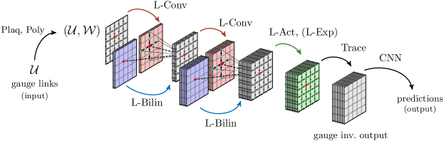
Figure 1: A possible realization of an L-CNN. Lattice data in the form of $\mathcal{U}$ links are first preprocessed by Plaq and Poly in order to generate elementary locally transforming $\mathcal{W}$ objects. An L-Conv is used to parallel transport nearby $\mathcal{W}$ objects (green dots) along the coordinate axes to a particular lattice site (red dot). An L-Bilin combines two layers by forming products of locally transforming objects which are stored in an increasing number of channels (indicated by stacked lattices). The second input layer (blue) for this operation can be a duplicate of the original layer (red). An additional L-Act (L-Exp) can modify $\mathcal{W}$ ($\mathcal{U}$) in a gauge equivariant way (green layer). A Trace layer generates gauge invariant output that can be further processed by a traditional CNN. The example depicts a 1+1D lattice but applies to higher dimensions as well. The basic layers presented can be combined to form other deeper network architectures.

Lattice gauge theory is a discretization of Yang-Mills theory Wilson (1974); Gattringer and Lang (2010); Smit (2002). We consider a system at finite temperature with gauge group $\mathrm{SU}(N_{c})$ in $D+1$ dimensions on a lattice $\Lambda$ of size $N_{t}\cdot N_{s}^{D}$ with $N_{t}$ ($N_{s}$) cells along the imaginary time (spatial) direction(s) with periodic boundary conditions. The link variables $U_{x,\mu}$ specify the parallel transport from a lattice site $x$ to its neighbor $x+\mu\equiv x+a\hat{e}^{\mu}$ with lattice spacing $a$. Gauge links transform according to

$$T_{\Omega}U_{x,\mu}=\Omega_{x}U_{x,\mu}\Omega^{\dagger}_{x+\mu},$$ (1)

where the group elements $\Omega_{x}$ are unitary and have unit determinant. The Yang-Mills action can be approximated by the Wilson action Wilson (1974)

$$S_{W}[U]=\frac{2}{g^{2}}\sum_{x\in\Lambda}\sum_{\mu<\nu}\mathrm{Re}\,\mathrm{Tr}\left[\mathbb{1}-U_{x,\mu\nu}\right]$$ (2)

with the plaquette variables

$$U_{x,\mu\nu}=U_{x,\mu}U_{x+\mu,\nu}U^{\dagger}_{x+\nu,\mu}U^{\dagger}_{x,\nu}=\vbox{\hbox{\includegraphics[scale={0.7}]{wilson_1.pdf}}}$$ (3)

which are $1\times 1$ (untraced) Wilson loops on the lattice. Unless specified otherwise, we assume Wilson loops to be untraced, i.e. matrix valued. The plaquette variables transform locally at $x$ as $T_{\Omega}U_{x,\mu\nu}=\Omega_{x}U_{x,\mu\nu}\Omega^{\dagger}_{x}.$

L-CNNs can express a large class of possible gauge equivariant functions in the lattice gauge theory framework. As customary in feed-forward CNNs, we split L-CNNs into more elementary “layers”, see Fig. 1. As input data for a layer we use a tuple $(\mathcal{U},\mathcal{W})$ consisting of non-locally transforming gauge link variables $\mathcal{U}$ and locally transforming variables $\mathcal{W}$. The first part of the tuple is the set of variables $\mathcal{U}=\{U_{x,\mu}\}$, which transform according to Eq. (1). For concreteness, we choose the defining (or fundamental) representation of $\mathrm{SU}(N_{c})$ such that we can treat link variables as complex special unitary $N_{c}\times N_{c}$ matrices. Its second part is a set of variables $\mathcal{W}=\{W_{x,i}\}$ with $W_{x,i}\in\mathbb{C}^{N_{c}\times N_{c}}$ and index $1\leq i\leq N_{\mathrm{ch}}$, which we interpret as “channels”. We require these additional input variables to transform locally at $x$:

$$T_{\Omega}W_{x,i}=\Omega_{x}W_{x,i}\Omega^{\dagger}_{x}.$$ (4)

A function $f$ that performs some mathematical operation on $(\mathcal{U},\mathcal{W})$ is called gauge equivariant (or gauge covariant) if $f(T_{\Omega}\mathcal{U},T_{\Omega}\mathcal{W})=T^{\prime}_{\Omega}f(\mathcal{U},\mathcal{W})$, where $T^{\prime}_{\Omega}f$ denotes the gauge transformed expression of the function $f$. Additionally, a function $f$ is gauge invariant if $f(T_{\Omega}\mathcal{U},T_{\Omega}\mathcal{W})=f(\mathcal{U},\mathcal{W})$. All possible functions that can be expressed as L-CNNs should either be equivariant or invariant.

LGE convolutions (L-Conv) perform a parallel transport of $\mathcal{W}$ objects at neighboring sites to the current location. They can be written as

$$W_{x,i}\rightarrow\sum_{j,\mu,k}\omega_{i,j,\mu,k}U_{x,k\cdot\mu}W_{x+k\cdot\mu,j}U^{\dagger}_{x,k\cdot\mu},$$ (5)

where $\omega_{i,j,\mu,k}\in\mathbb{C}$ are the weights of the convolution with $1\leq i\leq N_{\mathrm{ch,out}}$, $1\leq j\leq N_{\mathrm{ch,in}}$, $0\leq\mu\leq D$ and $-K$$\leq k\leq K$, where $K$ is the kernel size. Unlike traditional convolutional layers, the gauge equivariant kernels connect to other lattice sites only along the coordinate axes. The reason is path dependence. In the continuum case a natural choice would be the shortest path (or geodesic) connecting $x$ and $y$, which is also used for gauge equivariant neural networks that are formulated on manifolds Cohen et al. (2019). However, in our lattice approach the shortest path is not unique, unless one restricts oneself to the coordinate axes. Possible variations of this layer are to include an additional bias term, or to restrict to even sparser dilated convolutions Yu and Koltun (2016).

LGE bilinear layers (L-Bilin) combine two tuples $(\mathcal{U},\mathcal{W})$ and $(\mathcal{U},\mathcal{W}^{\prime})$ to form products of locally transforming quantities as

$$W_{x,i}\rightarrow\sum_{j,k}\alpha_{i,j,k}W_{x,j}W^{\prime}_{x,k},$$ (6)

where $\alpha_{i,j,k}\in\mathbb{C}$ are parameters with $1\leq i\leq N_{\mathrm{out}}$, $1\leq j\leq N_{\mathrm{in,1}}$ and $1\leq k\leq N_{\mathrm{in,2}}$. Since only locally transforming terms are multiplied in Eq. (6), gauge equivariance holds. For more flexibility, the bilinear operation can be further generalized by enlarging $\mathcal{W}$ and $\mathcal{W}^{\prime}$ to also include the unit element $\mathbb{1}$ and all Hermitian conjugates of $\mathcal{W}$ and $\mathcal{W}^{\prime}$. An L-Bilin can then also act as residual module He et al. (2016) and includes a bias term.

LGE activation functions (L-Act) can be applied at each lattice site via

$$W_{x,i}\rightarrow g_{x,i}(\mathcal{U},\mathcal{W})W_{x,i}$$ (7)

using any scalar-valued, gauge invariant function $g$. A gauge equivariant generalization of the commonly used rectified linear unit (ReLU) could be realized by choosing $g_{x,i}(\mathcal{U},\mathcal{W})=\mathrm{ReLU}(\mathrm{Re}\,\mathrm{Tr}\left[W_{x,i}\right])$ where $g$ only depends on local variables. In general, $g$ can depend on values of variables at any lattice site and, in principle, could also depend on trainable parameters.

LGE exponentiation layers (L-Exp) can be used to update the link variables through

$$U_{x,\mu}\rightarrow U^{\prime}_{x,\mu}=\mathcal{E}_{x,\mu}U_{x,\mu},$$ (8)

where $\mathcal{E}_{x,\mu}\in\mathrm{SU}(N_{c})$ is a group element which transforms locally $T_{\Omega}\mathcal{E}_{x,\mu}=\Omega_{x}\mathcal{E}_{x,\mu}\Omega^{\dagger}_{x}$. By this update, the unitarity (${U^{\prime}}^{\dagger}_{x,\mu}U^{\prime}_{x,\mu}=\mathbb{1}$) and determinant ($\det U^{\prime}_{x,\mu}=1$) constraints remain satisfied. A particular realization of $\mathcal{E}_{x,\mu}$ in terms of $\mathcal{W}$-variables is given by the exponential map

$$\mathcal{E}_{x,\mu}(\mathcal{W})=\exp{\left(i\sum_{i}\beta_{\mu,i}\left[W_{x,i}\right]_{\mathrm{ah}}\right)},$$ (9)

where $\left[W_{x,i}\right]_{\mathrm{ah}}$ denotes the anti-Hermitian traceless part of $W_{x,i}$, and $\beta_{\mu,i}\in\mathbb{R}$ are real-valued weight parameters with $0\leq\mu\leq D$ and $1\leq i\leq N_{\mathrm{ch}}$. The above method projects $W_{x,i}$ onto the Lie algebra, and therefore $\mathcal{E}_{x,\mu}$ is guaranteed to be an element of the Lie group.

Trace layers generate gauge invariant output

$$\mathcal{T}_{x,i}(\mathcal{U},\mathcal{W}) =\mathrm{Tr}\left[W_{x,i}\right].$$ (10)

Plaquette layers (Plaq) generate all possible plaquettes $U_{x,\mu\nu}$ from Eq. (3) at location $x$ and add them to $\mathcal{W}$ as a preprocessing step. To reduce redundancy, we can choose to only compute plaquettes with positive orientation, i.e. $U_{x,\mu\nu}$ with $\mu<\nu$.

Polyakov layers (Poly) compute all possible Polyakov loops Polyakov (1978) at every lattice site according to

$$\mathcal{L}_{x,\mu}(\mathcal{U})=\prod_{k}U_{x+k\cdot\mu,\mu}=U_{x,\mu}U_{x+\mu,\mu}\dots U_{x-\mu,\mu}$$ (11)

and add them to the set of locally transforming objects in $\mathcal{W}$ as a preprocessing step. These loops wrap around the periodic boundary of the (torus-like) space-time lattice and cannot be contracted to a single point.

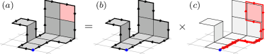
Figure 2: Sketch of the proof that L-CNNs can generate arbitrary Wilson loops. (a) An arbitrary contractible Wilson loop (depicted here in 3 dimensions) surrounds a surface that can be tessellated into $n$ tiles of $1\times 1$ unit lattice area. The blue dot indicates the starting point of the untraced Wilson loop. (b) A Wilson loop with $n$ tiles can be composed of an untraced Wilson loop with $n-1$ tiles and a path along the boundary to the missing tile using an L-Bilin. (c) An arbitrary return path to and from a $1\times 1$ plaquette is obtained by successive applications of L-Convs after an initial Plaq.

Figure 2 contains a sketch of the proof by induction that L-CNNs can generate arbitrary Wilson loops (Fig. 2a). This is achieved by concatenating loops as shown using an L-Bilin such that intermediate path segments to the origin (indicated by a blue dot in Fig. 2) cancel. Arbitrary paths to a plaquette and back along the same path as shown in Fig. 2c can be generated by an initial Plaq with repeated application of L-Convs. On topologies that are not simply connected, loops that cannot be contracted to a point can be added by Poly. The possibility of forming a complete Wilson loop basis Giles (1981); Loll (1993) together with the universality of deep convolutional neural networks Zhou (2018) makes L-CNNs capable of universal approximation within an equivalence class of gauge connections.

These layers can be assembled and applied to specific problems in lattice gauge theory. A possible architecture is depicted in Fig. 1. The alternated application of L-Conv and L-Bilin can double the area of loops. Repeating this block can grow Wilson loops to arbitrary size. L-Bilins are already non-linear, but even more general relations can be expressed through L-Acts. Building blocks in the form of L-Conv+L-Bilin+L-Act cover a wide range of possible gauge equivariant non-linear functions. The Trace layer renders the output gauge invariant so that it can be further processed by a conventional CNN or a multilayer perceptron (MLP) without spoiling gauge symmetry. Some applications, such as classical time evolution Ambjørn et al. (1991) or gradient flow Lüscher (2010), require operations that can change the set of gauge links  $\mathcal{U}$. This can be achieved using an L-Exp. After an L-Exp, one can use Plaq and Poly to update $\mathcal{W}$ accordingly.

We demonstrate the performance of L-CNNs by applying them to a number of seemingly simple regression problems. Specifically, we train L-CNN models using supervised learning to predict local, gauge invariant observables and make comparisons to traditional CNN models as a baseline test. We perform our experiments on data from 1+1D and 3+1D lattices with various sizes and coupling constants $g$, which we have generated using our own $\mathrm{SU}(2)$ Monte Carlo code based on the Metropolis algorithm Creutz (1980). One type of observable that we focus on is the real value of traced Wilson loops, i.e.

$$W^{(m\times n)}_{x,\mu\nu}=\frac{1}{N_{c}}\mathrm{Re}\,\mathrm{Tr}\left[U^{(m\times n)}_{x,\mu\nu}\right],$$ (12)

where $U^{(m\times n)}_{x,\mu\nu}$ is an $m\times n$ Wilson loop in the $\mu\nu$ plane. A second observable that we study, which is of more immediate physical relevance, is the topological charge density $q_{x}$, which is only available in 3+1D. In particular, we focus on the plaquette discretization given by

$$q^{\mathrm{plaq}}_{x}=\frac{\epsilon_{\mu\nu\rho\sigma}}{32\pi^{2}}\mathrm{Tr}\left[\frac{U_{x,\mu\nu}\!-\!U^{\dagger}_{x,\mu\nu}}{2i}\,\frac{U_{x,\rho\sigma}\!-\!U^{\dagger}_{x,\rho\sigma}}{2i}\right].$$ (13)

Our frameworks of choice are PyTorch and PyTorch Lightning. We have implemented the necessary layers discussed previously as modules in PyTorch, which can be used to assemble complete L-CNN models. Our code is open source and hosted on GitLab . In addition to gauge equivariance, we formulate our models to be translationally equivariant, which makes them applicable to arbitrary lattices. The task of the training procedure is to minimize a mean-squared error (MSE) loss function, which compares the prediction of the model to the ground truth from the dataset. For technical details, see our Supplementary Material.

Our L-CNN architectures consist of stacks of L-Conv+L-Bilin blocks, followed by a trace operation, as shown in Fig. 1. The gauge invariant output at each lattice site is mapped by linear layers to the final output nodes. We have experimented with architectures of various sizes, with the smallest models only consisting of a single L-Conv+L-Bilin layer and $\approx 100$ parameters to very large architectures with a stack of up to four layers of L-Conv+L-Bilin and $\approx 40,000$ trainable parameters.

For comparison, we implement gauge symmetry breaking baseline models using a typical CNN architecture. We use stacks of two-dimensional convolutions followed by non-linear activation functions (such as ReLU, LeakyReLU, $\tanh{}$ and sigmoid) and global average pooling Lin et al. (2013) before mapping to the output nodes using linear layers. Baseline architectures vary from just one or two convolutions with $\approx 300$ parameters to large models with up to six convolutions and $\approx 100,000$ trainable weight parameters. These models are trained and validated on small lattices ($8\cdot 8$ for 1+1D and $4\cdot 8^{3}$ for 3+1D, $10^{4}$ training and $10^{3}$ validation examples) but tested on data from larger lattices (up to $64\cdot 64$ and $8\cdot 16^{3}$, $10^{3}$ test examples). In total, we have trained $2680$ individual baseline models.

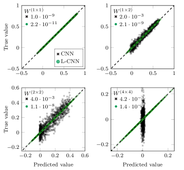
Figure 3: Scatter plots comparing best L-CNN models to baseline CNN models for Wilson loops of various sizes for 1+1D. For each example in the $N_{s}\cdot N_{t}=8\cdot 8$ test dataset, we plot the true value vs. the model prediction. Perfect agreement is indicated by the dashed $45^{\circ}$ line. As the size of the traced Wilson loops grows, the performance of the baseline CNN models worsens quickly. On the other hand, L-CNN models achieve high agreement in all cases. The values in the upper left corner denote the MSEs of each plot.

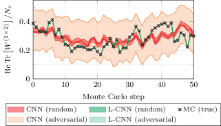
Figure 4: Prediction uncertainty in $W^{(1\times 2)}$ due to breaking of gauge symmetry for our best baseline CNN and L-CNN models on $8\cdot 8$ test data. Black crosses (MC) denote the calculated true value of the Wilson loop. The red bands show the effects of random gauge transformations and transformations obtained from adversarial attacks. Predictions by the L-CNN models are invariant by construction.

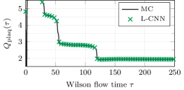
Figure 5: Predictions of our best L-CNN for the topological charge on a Wilson flowed $8\cdot 24^{3}$ lattice configuration at $2/g^{2}=0.2$.

A selection of results are presented in Figs. 3 and 4 for 1+1D and Fig. 5 for 3+1D lattices. Figure 3 shows scatter plots of our best performing models (L-CNN and baseline) evaluated on test data. We demonstrate that the performance of the baseline models quickly deteriorates with the growing size of the Wilson loop. In the case of $4\times 4$ loops, the baseline model collapses and only predicts the average value of the training data. This signals that the baseline models are unable to learn any meaningful relationship between input and output data. Except for the case of $1\times 1$ loops, the baseline CNN models are not able to adequately learn even moderately sized Wilson loops in 1+1D and have particular difficulty to predict negative values, which are associated with large gauge rotations.

We have experimented with different baseline CNN architectures of various widths and depths and a variety of activation functions. In all of our experiments we have obtained similar behaviour as shown in Fig. 3. In contrast, L-CNN architectures are able to converge to solutions that can predict the observables to a high degree of accuracy in all tasks, and they are gauge covariant by construction. Furthermore, our models perform well across all considered lattice sizes because of translational equivariance. In Fig. 4, we show how predictions of baseline CNNs and L-CNNs change under gauge transformations. We have tried two strategies: random gauge transformations and adversarial attacks (see our Supplementary Material Sec. VI.A). We observe that trained CNN models learn to approximate gauge invariance (see Boyda et al. (2021a) for a similar result) but are vulnerable to certain gauge transformations that can drastically change their predictions.

L-CNNs can also be applied to 3+1D lattices: Figure 5 demonstrates the predictions of our best L-CNN model for topological charge (trained on $4\cdot 8^{3}$) during Wilson (gradient) flow Lüscher (2010) on an $8\cdot 24^{3}$ lattice. The values from our simulation (MC) agree with the model predictions to high accuracy and assume integer values, as expected.

To summarize, we introduced a neural network structure for processing lattice gauge theory data that is capable of universal approximation within physically relevant degrees of freedom. The network achieves this by growing Wilson loops of arbitrary shapes in successive trainable gauge-covariant network layers. We demonstrated that our method surpasses ordinary convolutional networks in simple regression tasks on the lattice and that it manages to predict and generalize results for larger Wilson loops where a baseline network completely fails. Furthermore, our models can also be applied to lattices of any size without requiring retraining or transfer learning. From a broader perspective, we introduced a generalization of traditional CNNs that could replace them in a large range of machine learning applications where CNNs are applied to lattice gauge data.

Our approach opens up exciting possibilities for future research. So far, we implemented the network layers for the $\mathrm{SU}(2)$ gauge group only, but our method works for any $\mathrm{SU}(N_{c})$. Also, we have introduced the general concepts of Polyakov-loop generating layers and of exponentiation layers, but we have not exploited them in numerical experiments. It would be interesting to study these layers and their possible applications. Finally, the compositional nature of successive gauge-covariant network layers is reminiscent of the renormalization group picture Bény (2013); Mehta and Schwab (2014); Li and Wang (2018). Trainable networks could provide a viable implementation of the renormalization group approaches by Wilson Wilson (1980) and Symanzik Symanzik (1983). Improved lattice actions and operators could be obtained by training on coarse lattices, while providing ground-truth data from finer grained simulations. Automatically learning improved lattice actions could make accessible previously unreachable system sizes for zero and finite temperature applications Niedermayer (1997); Iwasaki (1985); Lagaë and Sinclair (1998) as well as for real-time lattice simulations Moore (1996); Ipp and Müller (2018, 2017, 2020).