Learning by Self-Explanation, with Application to Neural Architecture Search

Abstract

Learning by self-explanation is an effective learning technique in human learning, where students explain a learned topic to themselves for deepening their understanding of this topic. It is interesting to investigate whether this explanation-driven learning methodology broadly used by humans is helpful for improving machine learning as well. Based on this inspiration, we propose a novel machine learning method called learning by self-explanation (LeaSE). In our approach, an explainer model improves its learning ability by trying to clearly explain to an audience model regarding how a prediction outcome is made. LeaSE is formulated as a four-level optimization problem involving a sequence of four learning stages which are conducted end-to-end in a unified framework: 1) explainer learns; 2) explainer explains; 3) audience learns; 4) explainer re-learns based on the performance of the audience. We develop an efficient algorithm to solve the LeaSE problem. We apply LeaSE for neural architecture search on CIFAR-100, CIFAR-10, and ImageNet. Experimental results strongly demonstrate the effectiveness of our method.

1 Introduction

In humans’ learning practice, a broadly adopted learning skill is self-explanation where students explain to themselves a learned topic to achieve better understanding of this topic. Self-explanation encourages a student to actively digest and integrate prior knowledge and new information, which helps to fill in the gaps in understanding a topic. It has shown considerable effectiveness in improving learning outcomes.

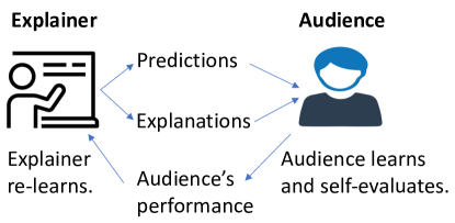
Figure 1: Illustration of learning by self-explanation. An explainer explains to the audience regarding how predictions are made. The audience leverages the explanations to learn and evaluates itself. Performance of the audience acts as feedback to guide the explainer to re-learn for giving better explanations. This process repeats until the audience’s performance is good enough.

We are interested in asking: can the explanation-driven learning method be borrowed from humans to help machines to learn better? Motivated by this inspiration, we propose a novel machine learning framework called learning by self-explanation (LeaSE) (as illustrated in Figure 1). In this framework, there is an explainer model and an audience model. They both learn to undertake the same ML task, such as image classification. The explainer has a learnable architecture and a set of learnable network weights. The audience has a predefined architecture by human experts and a set of learnable network weights. The goal is to help the explainer to learn well on the target task. The way to achieve this goal is to encourage the explainer to give clear explanations to the audience regarding how predictions are made. Intuitively, if a model can explain prediction outcomes well, it must have a deep understanding of the prediction task and can learn better based on this understanding. The learning is organized into four stages. In the first stage, the explainer trains its network weights by minimizing the prediction loss on its training dataset, with its architecture fixed. In the second stage, the explainer uses its model trained in the first stage to make predictions on the training data examples of the audience and leverages an adversarial attack (Goodfellow et al., 2014; Etmann et al., 2019) approach to explain the prediction outcomes. In the third stage, the audience model combines its training examples and the explainer-made explanations of prediction outcomes on these examples to train its network weights. In the fourth stage, the explainer updates its neural architecture by minimizing its validation loss and the audience’s validation loss. The fours stages are synthesized into a unified four-level optimization framework where they are performed jointly in an end-to-end manner. Each learning stage has an influence on other stages. We apply our method for neural architecture search in image classification tasks. Our method achieves significant improvement on CIFAR-100, CIFAR-10, and ImageNet (Deng et al., 2009).

The major contributions of this paper are as follows:

• Drawing inspiration from the explanation-driven learning technique of humans, we propose a novel machine learning approach called learning by self-explanation (LeaSE). In our approach, an explainer model improves its learning ability by trying to clearly explain to an audience model regarding how the prediction outcomes are made.

• We develop a multi-level optimization framework to formulate LeaSE which involves four stages of learning: explainer learns; explainer explains; audience learns; explainer re-learns based on the audience’s performance.

• We develop an efficient algorithm to solve the LeaSE problem.

• We apply LeaSE for neural architecture search on CIFAR-100, CIFAR-10, and ImageNet, where the results demonstrate the effectiveness of our method.

2 Related Works

2.1 Neural Architecture Search (NAS)

In the past few years, a wide variety of NAS methods have been proposed and achieved considerable success in automatically identifying highly-performing architectures of neural networks for the sake of reducing the reliance on human experts. Early NAS approaches (Zoph and Le, 2017; Pham et al., 2018; Zoph et al., 2018) are mostly based on reinforcement learning (RL) which use a policy network to generate architectures and evaluate these architectures on validation set. The validation loss is used as a reward to optimize the policy network and train it to produce high-quality architectures. While RL-based approaches achieve the first wave of success in NAS research, they are computationally very expensive since evaluating the architectures requires a heavy-duty training process. This limitation renders RL-based approaches not applicable for most users who do not have enough computational resources. To address this issue, differentiable search methods (Cai et al., 2019; Liu et al., 2019; Xie et al., 2019) have been proposed, which parameterize architectures as differentiable functions and perform search using efficient gradient-based methods. In these methods, the search space of architectures is composed of a large set of building blocks where the output of each block is multiplied with a smooth variable indicating how important this block is. Under such a formulation, search becomes solving a mathematical optimization problem defined on the importance variables where the objective is to find out an optimal set of variables that yield the lowest validation loss. This optimization problem can be solved efficiently using gradient-based methods. Differentiable NAS research is initiated by DARTS (Liu et al., 2019) and further improved by subsequent works such as P-DARTS (Chen et al., 2019), PC-DARTS (Xu et al., 2020), etc. P-DARTS (Chen et al., 2019) grows the depth of architectures progressively in the search process. PC-DARTS (Xu et al., 2020) samples sub-architectures from a super network to reduce redundancy during search. Our proposed LeaSE framework is orthogonal to existing NAS methods and can be used in combination with any differentiable NAS method to further improve these methods. Such et al. (2019) proposed to learn a generative model to generate synthetic examples which are used to search the architecture of an auxiliary model. Our work differs from this one in that: 1) we focus on searching the architecture of a primary model (the explainer) by letting it explain to an auxiliary model (the audience) while (Such et al., 2019) focuses on searching the architecture of the auxiliary model; 2) our primary model produces explanations via adversarial attack while the generative model in (Such et al., 2019) generates synthetic examples. Besides RL-based approaches and differentiable NAS, another paradigm of NAS methods (Liu et al., 2018b; Real et al., 2019) are based on the evolutionary algorithm. In these methods, architectures are formulated as individuals in a population. High-quality architectures produce offspring to replace low-quality architectures, where the quality is measured using fitness scores. Similar to RL-based approaches, these methods also require considerable computing resources.

2.2 Interpretable Machine Learning

The explainability and transparency of machine learning models is crucial for mission-critical applications. Many approaches have been proposed for understanding the predictions made by black-box models. Many prior approaches for interpretable ML focus on finding out key evidence from the input data (such as phrases in texts and regions in images) that is most relevant to a prediction, then using these evidence to justify the meaningfulness of the prediction. In (Zeiler and Fergus, 2014) and (Zintgraf et al., 2017), the authors perform perturbation on the input data elements (e.g., pixels) and check which perturbed elements cause more changes of the output. Such elements are considered to be more relevant to the output and are used as explanations. In (Baehrens et al., 2010; Simonyan et al., 2013) and (Smilkov et al., 2017), the authors identify the contribution of each input feature to the output prediction by propagating the contribution through layers of a deep neural network. Another body of works (Yang et al., 2016; Mullenbach et al., 2018; Lei et al., 2016) are based on the idea of attention. While training the prediction model, an attention network is trained to calculate an attention score for each input data element. Elements with large attention scores are used as explanations. In (Yang et al., 2016), attention mechanisms are used to select important words and sentences for interpreting hierarchical recurrent networks. Mullenbach et al. (2018) leverage attention networks for explaining convolution networks. In addition, another widely adopted idea is to use simple but more interpretable models to interpret expressive black-box models. For example, in LIME (Ribeiro et al., 2016), an interpretable linear model is used to approximate the decision boundary of a black-box model at an interested instance and interpretation is performed by checking dominant features in the linear model. Our work differs from these existing works in that: existing works focus on interpreting a trained model while our method focuses on improving the training of a model by letting it explain. In other words, the goal of existing works is explaining while that of our work is learning. The interpretation module (in the second stage) in our framework can be any model-interpretation method.

The concept of self-explanation was investigated in (Elton, 2020), which calculates confidence levels for decisions and explanations based on mutual information. Different from our work, this work does not leverage self-explanation to improve model training. Alvarez-Melis and Jaakkola (2018) proposed a self-explaining network (SEN) which simultaneously outputs predictions and explanations. Our work differs from this one in that: our work uses the explanations generated by model A to train model B where B’s validation performance reflects how good A’s explanations are; the training of A is continuously improved so that it can generate good explanations. Leveraging another model to evaluate the quality of explanations made by one model is more robust and overfitting-resilient. In contrast, SEN learns to make predictions and explains prediction results in a single model, where the explanations may not be able to generalize in other models. Explanation-based learning (DeJong and Mooney, 1986; Minton, 1990) has been investigated in logic-based AI systems. These approaches require manual design of logic rules, which are not scalable.

Table 1: Notations in Learning by Self-Explanation

Notation	Meaning
$A$	Architecture of the explainer
$E$	Network weights of the explainer
$W$	Network weights of the audience
$\delta$	Explanations
$D_{e}^{(\textrm{tr})}$	Training data of the explainer
$D_{a}^{(\textrm{tr})}$	Training data of the audience
$D_{e}^{(\textrm{val})}$	Validation data of the explainer
$D_{a}^{(\textrm{val})}$	Validation data of the audience

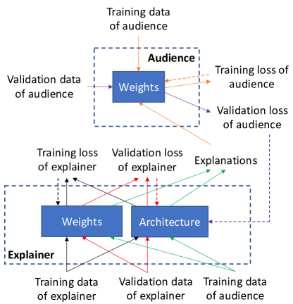
Figure 2: Learning by self-explanation. Following the solid arrows, predictions are made and training/validation losses are calculated. Following the dotted arrows, gradient updates of network weights and architecture variables are calculated and weights/architecture are updated.

3 Methods

In this section, we propose a four-level optimization framework to formulate learning by self-explanation (LeaSE) (as shown in Figure 2) and develop an optimization algorithm to solve the four-level optimization problem.

3.1 Learning by Self-Explanation

In the LeaSE framework, there is an explainer model and an audience model, both of which learn to perform the same target task. The primary goal of our framework is to help the explainer to learn the target task very well. The way to achieve this goal is to let the explainer make meaningful explanations of the prediction outcomes in the target task. The intuition behind LeaSE is: to correctly explain prediction results, a model needs to learn to understand the target task very well. The explainer has a learnable architecture $A$ and a set of learnable network weights $E$. The audience has a pre-defined neural architecture (by human experts) and a set of learnable network weights $W$. The learning is organized into four stages. In the first stage, the explainer trains its network weights $E$ on its training dataset $D_{e}^{(\textrm{tr})}$, with the architecture fixed:

$$E^{*}(A)=\textrm{min}_{E}\;L(E,A,D_{e}^{(\textrm{tr})}).$$ (1)

To define the training loss, we need to use the architecture $A$ together with network weights $W$ to make predictions on training examples. However, $A$ cannot be updated by minimizing the training loss. Otherwise, a trivial solution of $A$ will be yielded: $A$ is very large and complex that it can perfectly overfit the training data but will make largely incorrect predictions on novel data examples. Note that $E^{*}(A)$ is a function of $A$ for that $L(E,A,D_{e}^{(\textrm{tr})})$ is a function of $A$ and $E^{*}(A)$ depends on $L(E,A,D_{e}^{(\textrm{tr})})$. In the second stage, the explainer uses the trained model $E^{*}(A)$ to make predictions on the input training examples $D_{a}^{(\textrm{tr})}$ of the audience and explains the prediction outcomes. Specifically, given an input data example $x$ (without loss of generality, we assume it is an image) and the predicted label $y$, the explainer aims to find out a subset of image patches $P$ in $x$ that are mostly correlated with $y$ and uses $P$ as explanations for $y$. We leverage an adversarial attack approach (Goodfellow et al., 2014; Etmann et al., 2019) to achieve this goal. Adversarial attack adds small random perturbations $\delta$ to pixels in $x$ so that the prediction outcome on the perturbed image $x+\delta$ is no longer $y$. Pixels that are perturbed more have higher correlations with the prediction outcome $y$ and can be used as explanations. This process amounts to solving the following optimization problem:

$$\Delta^{*}(E^{*}(A))=\textrm{max}_{\Delta}\;\;\sum_{i=1}^{N}\ell(f(x_{i}+\delta_{i};{E^{*}(A)}),f(x_{i};{E^{*}(A)}))$$ (2)

where $\Delta=\{\delta_{i}\}_{i=1}^{N}$ and $\delta_{i}$ is the perturbation added to image $x_{i}$. $f(x_{i}+\delta_{i};{E^{*}(A)})$ and $f(x_{i};{E^{*}(A)})$ are the prediction outcomes of the explainer’s network $f(\cdot;{E^{*}(A)})$ on $x_{i}+\delta_{i}$ and $x_{i}$. Without loss of generality, we assume the task is image classification (with $K$ classes). Then $f(x_{i}+\delta_{i};{E^{*}(A)})$ and $f(x_{i};{E^{*}(A)})$ are both $K$-dimensional vectors containing prediction probabilities on the $K$ classes. $\ell(\cdot,\cdot)$ is the cross-entropy loss with $\ell(\mathbf{a},\mathbf{b})=-\sum_{k=1}^{K}b_{i}\log a_{i}$. In this optimization problem, the explainer aims to find out perturbations for each image so that the predicted outcome on the perturbed image is largely different from that on the original image. The learned optimal perturbations are used as explanations and those with larger values indicate that the corresponding pixels are more important in decision-making. $\Delta^{*}(E^{*}(A))$ is a function of $E^{*}(A)$ since $\Delta^{*}(E^{*}(A))$ is a function of the objective in Eq.(2) and the objective is a function of $E^{*}(A)$. In the third stage, given the explanations $\Delta^{*}(E^{*}(A))$ made by the explainer, the audience leverages them to learn the target task. Since the perturbations indicate how important the input pixels are, the audience uses them to reweigh the pixels: $x\odot\delta$, where $\odot$ denotes element-wise multiplication. Pixels that are more important are given more weights. Then the audience trains its network weights on these weighted images:

$$W^{*}(\Delta^{*}(E^{*}(A)))=\textrm{min}_{W}\;\;\sum_{i=1}^{N}\ell(f(\delta_{i}^{*}(E^{*}(A))\odot x_{i};W),t_{i}),$$ (3)

where $f(\delta_{i}^{*}(E^{*}(A))\odot x_{i};W)$ is the prediction outcome of the audience’s network $f(\cdot;W)$ on the weighted image $\delta_{i}^{*}(E^{*}(A))\odot x_{i}$ and $t_{i}$ is the class label. $W^{*}(\Delta^{*}(E^{*}(A)))$ is a function of $\Delta^{*}(E^{*}(A))$ since $W^{*}(\Delta^{*}(E^{*}(A)))$ is a function of the objective in Eq.(3) and the objective is a function of $\Delta^{*}(E^{*}(A))$. In the fourth stage, the explainer validates its network weights $E^{*}(A)$ on its validation set $D^{(\textrm{val})}_{e}$ and the audience validates its network weights $W^{*}(\Delta^{*}(E^{*}(A)))$ on its validation set $D^{(\textrm{val})}_{a}$. The explainer optimizes its architecture by minimizing its validation loss and the audience’s validation loss:

$$\textrm{min}_{A}\;L(E^{*}(A),A,D_{e}^{(\textrm{val})})+\gamma L(W^{*}(\Delta^{*}(E^{*}(A))),D_{a}^{(\textrm{val})}),$$ (4)

where $\gamma$ is a tradeoff parameter.

We integrate the four stages in a unified four-level optimization framework and obtain the following formulation of LeaSE:

$$\begin{array}[]{l}\underset{A}{\textrm{min}}\;\;\;L(E^{*}(A),A,D_{e}^{(\textrm{val})})+\gamma L(W^{*}(\Delta^{*}(E^{*}(A))),D_{a}^{(\textrm{val})})\\ s.t.\;\;\;W^{*}(\Delta^{*}(E^{*}(A)))=\underset{W}{\textrm{min}}\;\;\sum\limits_{i=1}^{N}\ell(f(\delta_{i}^{*}(E^{*}(A))\odot x_{i};W),t_{i})\\ \quad\quad\Delta^{*}(E^{*}(A))=\underset{\Delta}{\textrm{max}}\;\;\sum\limits_{i=1}^{N}\ell(f(x_{i}+\delta_{i};{E^{*}(A)}),f(x_{i};{E^{*}(A)}))\\ \quad\quad E^{*}(A)=\underset{E}{\textrm{min}}\;L(E,A,D_{e}^{(\textrm{tr})}).\end{array}$$ (5)

In this framework, there are four optimization problems, each corresponding to a learning stage. From bottom to up, the optimization problems correspond to learning stage 1, 2, 3, and 4 respectively. The first three optimization problems are nested on the constraint of the fourth optimization problem. These four stages are conducted end-to-end in this unified framework. The solution $E^{*}(A)$ obtained in the first stage is used to perform explanation in the second stage. The explanations $\Delta^{*}(E^{*}(A))$ obtained in the second stage are used to train the model in the third stage. The solutions obtained in the first and third stage are used to make predictions on the fourth stage. The architecture $A$ updated in the fourth stage changes the training loss in the first stage and consequently changes the solution $E^{*}(A)$, which subsequently changes $\Delta^{*}(E^{*}(A))$ and $W^{*}(\Delta^{*}(E^{*}(A)))$. Following (Liu et al., 2019), we perform differentiable search on $A$ in a search space composed of candidate building blocks. Searching amounts to selecting a subset of candidate blocks by learning a selection variable for each block. The selection variables indicate the importance of individual blocks and are differentiable.

4 Optimization Algorithm

We develop an efficient algorithm to solve the LeaSE problem. Getting insights from (Liu et al., 2019), we calculate the gradient of $L(E,A,D_{e}^{(\textrm{tr})})$ w.r.t $E$ and approximate $E^{*}(A)$ using one-step gradient descent update of $E$. We plug the approximation $E^{\prime}$ of $E^{*}(A)$ into $\sum_{i=1}^{N}\ell(f(x_{i}+\delta_{i};{E^{*}(A)}),f(x_{i};{E^{*}(A)}))$ and obtain an approximated objective denoted by $O_{\Delta}$. Then we approximate $\Delta^{*}(E^{*}(A))$ using one-step gradient descent update of $\Delta$ based on the gradient of $O_{\Delta}$. Next, we plug the approximation $\Delta^{\prime}$ of $\Delta^{*}(E^{*}(A))$ into $\sum_{i=1}^{N}\ell(f(\delta_{i}^{*}(E^{*}(A))\odot x_{i};W),t_{i})$ and get another approximated objective denoted by $O_{W}$. Then we approximate $W^{*}(\Delta^{*}(E^{*}(A)))$ using one-step gradient descent update of $W$ based on the gradient of $O_{W}$. Finally, we plug the approximation $E^{\prime}$ of $E^{*}(A)$ and the approximation $W^{\prime}$ of $W^{*}(\Delta^{*}(E^{*}(A)))$ into $L(E^{*}(A),A,D_{e}^{(\textrm{val})})+\gamma L(W^{*}(\Delta^{*}(E^{*}(A))),D_{a}^{(\textrm{val})})$ and get the third approximated objective denoted by $O_{A}$. $A$ is updated by descending the gradient of $O_{A}$. In the sequel, we use $\nabla^{2}_{Y,X}f(X,Y)$ to denote $\frac{\partial f(X,Y)}{\partial X\partial Y}$.

First of all, we approximate $E^{*}(A)$ using

$$E^{\prime}=E-\xi_{e}\nabla_{E}L(E,A,D_{e}^{(\mathrm{tr})})$$ (6)

where $\xi_{e}$ is a learning rate. Plugging $E^{\prime}$ into $\sum_{i=1}^{N}\ell(f(x_{i}+\delta_{i};{E^{*}(A)}),f(x_{i};{E^{*}(A)}))$, we obtain an approximated objective $O_{\Delta}=\sum_{i=1}^{N}\ell(f(x_{i}+\delta_{i};E^{\prime}),f(x_{i};E^{\prime}))$. Then we approximate $\Delta^{*}(E^{*}(A))$ using one-step gradient descent update of $\Delta$ with respect to $O_{\Delta}$:

$$\Delta^{\prime}=\Delta-\xi_{\Delta}\nabla_{\Delta}(\sum\limits_{i=1}^{N}\ell(f(x_{i}+\delta_{i};E^{\prime}),f(x_{i};E^{\prime}))).$$ (7)

Plugging $\Delta^{\prime}$ into $\sum_{i=1}^{N}\ell(f(\delta_{i}^{*}(E^{*}(A))\odot x_{i};W),t_{i})$, we obtain an approximated objective $O_{W}=\sum_{i=1}^{N}\ell(f(\delta^{\prime}_{i}\odot x_{i};W),t_{i})$. Then we approximate $W^{*}(\Delta^{*}(E^{*}(A)))$ using one-step gradient descent update of $W$ with respect to $O_{W}$:

$$W^{\prime}=W-\xi_{W}\nabla_{w}(\sum\limits_{i=1}^{N}\ell(f(\delta^{\prime}_{i}\odot x_{i};W),t_{i})).$$ (8)

Finally, we plug $E^{\prime}$ and $W^{\prime}$ into $L(E^{*}(A),D_{e}^{(\textrm{val})})+\gamma L(W^{*}(\Delta^{*}(E^{*}(A))),D_{a}^{(\textrm{val})})$ and get $O_{A}=L(E^{\prime},D_{e}^{(\textrm{val})})+\gamma L(W^{\prime},D_{a}^{(\textrm{val})})$. We can update the explainer’s architecture $A$ by descending the gradient of $O_{A}$ w.r.t $A$:

$$\begin{array}[]{l}A\leftarrow A-\eta(\nabla_{A}L(E^{\prime},D_{e}^{(\textrm{val})})+\gamma\nabla_{A}L(W^{\prime},D_{a}^{(\textrm{val})}))\end{array}$$ (9)

where

$$\begin{array}[]{l}\nabla_{A}L(E^{\prime},A,D_{e}^{(\textrm{val})})=\\ \nabla_{A}L(E-\xi_{e}\nabla_{E}L(E,A,D_{e}^{(\mathrm{tr})}),A,D_{e}^{(\textrm{val})})=\\ -\xi_{e}\nabla^{2}_{A,E}L(E,A,D_{e}^{(\mathrm{tr})})\nabla_{E^{\prime}}L(E^{\prime},A,D_{e}^{(\textrm{val})})+\nabla_{A}L(E^{\prime},A,D_{e}^{(\textrm{val})})\end{array}$$ (10)

The first term in the third line involves expensive matrix-vector product, whose computational complexity can be reduced by a finite difference approximation:

$$\begin{array}[]{ll}\nabla_{A,E}^{2}L(E,A,D_{e}^{(\mathrm{tr})})\nabla_{E^{\prime}}L(E^{\prime},A,D_{e}^{(\textrm{val})})\approx\frac{1}{2\alpha}(\nabla_{A}L(E^{+},A,D_{e}^{(\mathrm{tr})})-\nabla_{A}L(E^{-},A,D_{e}^{(\mathrm{tr})})),\end{array}$$ (11)

where $E^{\pm}=E\pm\alpha\nabla_{E^{\prime}}L(E^{\prime},A,D_{e}^{(\textrm{val})})$ and $\alpha$ is a small scalar that equals $0.01/\|\nabla_{E^{\prime}}L(E^{\prime},A,$
$D_{e}^{(\textrm{val})})\|_{2}$.

For $\nabla_{A}L(W^{\prime},D_{a}^{(\textrm{val})})$ in Eq.(9), it can be calculated as $\frac{\partial E^{\prime}}{\partial A}\frac{\partial\Delta^{\prime}}{\partial E^{\prime}}\frac{\partial W^{\prime}}{\partial\Delta^{\prime}}\nabla_{W^{\prime}}L(W^{\prime},D_{a}^{(\textrm{val})})$ according to the chain rule, where

$$\frac{\partial W^{\prime}}{\partial\Delta^{\prime}} =\frac{\partial(W-\xi_{w}\nabla_{W}(\sum_{i=1}^{N}\ell(f(\delta^{\prime}_{i}\odot x_{i};W),t_{i})))}{\partial\Delta^{\prime}}$$ (12)

$$=-\xi_{W}\nabla^{2}_{\Delta^{\prime},W}(\sum_{i=1}^{N}\ell(f(\delta^{\prime}_{i}\odot x_{i};W),t_{i})),$$ (13)

$$\frac{\partial\Delta^{\prime}}{\partial E^{\prime}} =\frac{\partial(\Delta-\xi_{\Delta}\nabla_{\Delta}(\sum\limits_{i=1}^{N}\ell(f(x_{i}+\delta_{i};E^{\prime}),f(x_{i};E^{\prime}))))}{\partial E^{\prime}}$$ (14)

$$=-\xi_{\Delta}\nabla^{2}_{E^{\prime},\Delta}(\sum\limits_{i=1}^{N}\ell(f(x_{i}+\delta_{i};E^{\prime}),f(x_{i};E^{\prime}))),$$ (15)

and

$$\frac{\partial E^{\prime}}{\partial A} =\frac{\partial(E-\xi_{e}\nabla_{E}L(E,A,D_{e}^{(\mathrm{tr})}))}{\partial A}$$ (16)

$$=-\xi_{e}\nabla^{2}_{A,E}L(E,A,D_{e}^{(\mathrm{tr})}).$$ (17)

This algorithm is summarized in Algorithm 1.

while not converged do

       1. Update the explainer’s weights $E$ using Eq.(6)
2. Update the explanations $\Delta$ using Eq.(7)
2. Update the audience’s weights $W$ using Eq.(8)
3. Update the explainer’s architecture $A$ using Eq.(9)

end while

Algorithm 1 Optimization algorithm for learning by self-explanation

5 Experiments

In the experiments, we apply our proposed LeaSE framework to perform neural architecture search for image classification. Each experiment consists of two phrases: architecture search and evaluation. In the search phrase, an optimal cell is identified. In the evaluation phrase, multiple copies of the optimal cell are stacked into a larger network, which is retrained from scratch.

5.1 Datasets

The experiments are performed on three datasets, including CIFAR-10, CIFAR-100, and ImageNet (Deng et al., 2009). Both CIFAR-10 and CIFAR-100 contain 60K images from 10 classes (each class has the same number of images). For each of them, we split it into a training set with 25K images, a validation set with 25K images, and a test set with 10K images. During architecture search in LeaSE, the training set is used as $D_{e}^{(\textrm{tr})}$ and $D_{a}^{(\textrm{tr})}$ and the validation set is used as $D_{e}^{(\textrm{val})}$ and $D_{a}^{(\textrm{val})}$. During architecture evaluation, the composed large network is trained on the combination of $D_{e}^{(\textrm{tr})}$ and $D_{a}^{(\textrm{tr})}$. ImageNet contains 1.2M training images and 50K test images, coming from 1000 objective classes. Performing architecture search on the 1.2M images is computationally too costly. To address this issue, following (Xu et al., 2020), we randomly sample 10% images from the 1.2M images to form a new training set and another 2.5% images to form a validation set, then perform search on them. During architecture evaluation, the composed large network is trained on the entire set of 1.2M images.

5.2 Experimental Settings

Our framework is orthogonal to existing NAS approaches and can be applied to any differentiable NAS method. In the experiments, LeaSE was applied to DARTS (Liu et al., 2019), P-DARTS (Chen et al., 2019), and PC-DARTS (Xu et al., 2020). The search spaces of these methods are composed of (dilated) separable convolutions with sizes of $3\times 3$ and $5\times 5$, max pooling with size of $3\times 3$, average pooling with size of $3\times 3$, identity, and zero. Each LeaSE experiment was repeated for ten times with different random seeds. The mean and standard deviation of classification errors obtained from the 10 runs are reported.

During architecture search, for CIFAR-10 and CIFAR-100, the architecture of the explainer is a stack of 8 cells. Each cell consists of 7 nodes. We set the initial channel number to 16. For the architecture of the audience model, we experimented with ResNet-18 and ResNet-50 (He et al., 2016b). We set the tradeoff parameter $\gamma$ to 1. The search algorithm was based on SGD, with a batch size of 64, an initial learning rate of 0.025 (reduced in later epochs using a cosine decay scheduler), an epoch number of 50, a weight decay of 3e-4, and a momentum of 0.9. The rest of hyperparameters mostly follow those in DARTS, P-DARTS, and PC-DARTS.

During architecture evaluation, for CIFAR-10 and CIFAR-100, a larger network of the explainer is formed by stacking 20 copies of the searched cell. The initial channel number was set to 36. We trained the network with a batch size of 96, an epoch number of 600, on a single Tesla v100 GPU. On ImageNet, we evaluate two types of architectures: 1) those searched on a subset of ImageNet; 2) those searched on CIFAR-10 or CIFAR-100. In either type, 14 copies of optimally searched cells are stacked into a large network, which was trained using eight Tesla v100 GPUs on the 1.2M training images, with a batch size of 1024 and an epoch number of 250. Initial channel number was set to 48.

5.3 Results

Table 2: Test error on CIFAR-100, number of model weights (millions), and search cost (GPU days on a Tesla v100). DARTS-1st and DARTS-2nd represents that first-order and second-order approximation is used in DARTS’ optimization algorithm. LeaSE-R18-DARTS1st represents that the manually-designed architecture in the audience model is ResNet-18 and the search space is the same as that in DARTS-1st. Similar meanings hold for other notations in such a format. R50 denotes ResNet-50. Results marked with * are obtained from DARTS^- (Chu et al., 2020a). Methods marked with ${\dagger}$ were re-run for 10 times. For DARTS⁺ marked with $\Delta$, we ran it for 600 epochs instead of 2000 epochs (used in (Liang et al., 2019)) in the architecture evaluation stage, to ensure the comparison with other methods (running 600 epochs) is fair.

Method	Error(%)	Param(M)	Cost
*ResNet (He et al., 2016a)	22.10	1.7	-
DenseNet (Huang et al., 2017)	17.18	25.6	-
*PNAS (Liu et al., 2018a)	19.53	3.2	150
ENAS (Pham et al., 2018)	19.43	4.6	0.5
AmoebaNet (Real et al., 2019)	18.93	3.1	3150
*GDAS (Dong and Yang, 2019)	18.38	3.4	0.2
R-DARTS (Zela et al., 2020)	18.01$\pm$0.26	-	1.6
DARTS- (Chu et al., 2020a)	17.51$\pm$0.25	3.3	0.4
†DARTS- (Chu et al., 2020a)	18.97$\pm$0.16	3.1	0.4
ΔDARTS+ (Liang et al., 2019)	17.11$\pm$0.43	3.8	0.2
DropNAS (Hong et al., 2020)	16.39	4.4	0.7
†DARTS-1st (Liu et al., 2019)	20.52$\pm$0.31	3.5	1.0
LeaSE-RN18-DARTS1st (ours)	17.04$\pm$0.10	3.6	1.1
LeaSE-RN50-DARTS1st (ours)	16.87$\pm$0.08	3.6	1.2
*DARTS-2nd (Liu et al., 2019)	20.58$\pm$0.44	3.5	1.5
LeaSE-RN18-DARTS2nd (ours)	16.80$\pm$0.17	3.7	1.7
LeaSE-RN50-DARTS2nd (ours)	16.39$\pm$0.07	3.6	1.9
${\dagger}$PC-DARTS (Xu et al., 2020)	17.96$\pm$0.15	3.9	0.1
LeaSE-RN18-PCDARTS (ours)	16.39$\pm$0.21	4.0	0.5
LeaSE-RN50-PCDARTS (ours)	16.17$\pm$0.05	3.9	0.7
*P-DARTS (Chen et al., 2019)	17.49	3.6	0.3
LeaSE-RN18-PDARTS (ours)	15.23$\pm$0.11	3.7	0.8
LeaSE-RN50-PDARTS (ours)	15.13$\pm$0.07	3.6	1.0

Table 3: Test error on CIFAR-10, number of model weights (millions), and search cost (GPU days on a Tesla v100). Results marked with * are obtained from DARTS^- (Chu et al., 2020a), NoisyDARTS (Chu et al., 2020b), and DrNAS (Chen et al., 2020). The rest notations are the same as those in Table 2.

Method Error(%) Param(M) Cost *DenseNet (Huang et al., 2017) 3.46 25.6 - *HierEvol (Liu et al., 2018b) 3.75$\pm$0.12 15.7 300 NAONet-WS (Luo et al., 2018) 3.53 3.1 0.4 PNAS (Liu et al., 2018a) 3.41$\pm$0.09 3.2 225 ENAS (Pham et al., 2018) 2.89 4.6 0.5 NASNet-A (Zoph et al., 2018) 2.65 3.3 1800 AmoebaNet-B (Real et al., 2019) 2.55$\pm$0.05 2.8 3150 *R-DARTS (Zela et al., 2020) 2.95$\pm$0.21 - 1.6 GDAS (Dong and Yang, 2019) 2.93 3.4 0.2 GTN (Such et al., 2019) 2.92$\pm$0.06 8.2 0.67 SNAS (Xie et al., 2019) 2.85 2.8 1.5 ^ΔDARTS⁺ (Liang et al., 2019) 2.83$\pm$0.05 3.7 0.4 BayesNAS (Zhou et al., 2019) 2.81$\pm$0.04 3.4 0.2 MergeNAS (Wang et al., 2020) 2.73$\pm$0.02 2.9 0.2 NoisyDARTS (Chu et al., 2020b) 2.70$\pm$0.23 3.3 0.4 ASAP (Noy et al., 2020) 2.68$\pm$0.11 2.5 0.2 SDARTS (Chen and Hsieh, 2020) 2.61$\pm$0.02 3.3 1.3 DARTS^- (Chu et al., 2020a) 2.59$\pm$0.08 3.5 0.4 ^†DARTS^- (Chu et al., 2020a) 2.97$\pm$0.04 3.3 0.4 DropNAS (Hong et al., 2020) 2.58$\pm$0.14 4.1 0.6 PC-DARTS (Xu et al., 2020) 2.57$\pm$0.07 3.6 0.1 FairDARTS (Chu et al., 2019) 2.54 3.3 0.4 DrNAS (Chen et al., 2020) 2.54$\pm$0.03 4.0 0.4 *DARTS-1st (Liu et al., 2019) 3.00$\pm$0.14 3.3 0.4   LeaSE-R18-DARTS1st (ours) 2.85$\pm$0.09 3.4 0.6   LeaSE-R50-DARTS1st (ours) 2.76$\pm$0.03 3.3 0.7 *DARTS-2nd (Liu et al., 2019) 2.76$\pm$0.09 3.3 1.5   LeaSE-R18-DARTS2nd (ours) 2.59$\pm$0.06 3.3 1.5   LeaSE-R50-DARTS2nd (ours) 2.52$\pm$0.04 3.4 1.7 *PC-DARTS (Xu et al., 2020) 2.57$\pm$0.07 3.6 0.1   LeaSE-R18-PC-DARTS (ours) 2.50$\pm$0.04 3.7 0.4   LeaSE-R50-PC-DARTS (ours) 2.48$\pm$0.02 3.7 0.5 *P-DARTS (Chen et al., 2019) 2.50 3.4 0.3   LeaSE-R18-PDARTS (ours) 2.45$\pm$0.03 3.4 0.8   LeaSE-R50-PDARTS (ours) 2.44$\pm$0.03 3.4 1.0

Table 4: Top-1 and top-5 classification errors on the test set of ImageNet, number of model parameters (millions) and search cost (GPU days). Results marked with * are obtained from DARTS^- (Chu et al., 2020a) and DrNAS (Chen et al., 2020). The rest notations are the same as those in Table 2. From top to bottom, on the first three blocks are 1) networks manually designed by humans; 2) non-gradient based NAS methods; and 3) gradient-based NAS methods.

Method Top-1 Top-5 Param Cost Error (%) Error (%) (M) (GPU days) *Inception-v1 (Szegedy et al., 2015) 30.2 10.1 6.6 - MobileNet (Howard et al., 2017) 29.4 10.5 4.2 - ShuffleNet 2$\times$ (v1) (Zhang et al., 2018) 26.4 10.2 5.4 - ShuffleNet 2$\times$ (v2) (Ma et al., 2018) 25.1 7.6 7.4 - *NASNet-A (Zoph et al., 2018) 26.0 8.4 5.3 1800 PNAS (Liu et al., 2018a) 25.8 8.1 5.1 225 MnasNet-92 (Tan et al., 2019) 25.2 8.0 4.4 1667 AmoebaNet-C (Real et al., 2019) 24.3 7.6 6.4 3150 *SNAS-CIFAR10 (Xie et al., 2019) 27.3 9.2 4.3 1.5 BayesNAS-CIFAR10 (Zhou et al., 2019) 26.5 8.9 3.9 0.2 PARSEC-CIFAR10 (Casale et al., 2019) 26.0 8.4 5.6 1.0 GDAS-CIFAR10 (Dong and Yang, 2019) 26.0 8.5 5.3 0.2 DSNAS-ImageNet (Hu et al., 2020) 25.7 8.1 - - SDARTS-ADV-CIFAR10 (Chen and Hsieh, 2020) 25.2 7.8 5.4 1.3 PC-DARTS-CIFAR10 (Xu et al., 2020) 25.1 7.8 5.3 0.1 ProxylessNAS-ImageNet (Cai et al., 2019) 24.9 7.5 7.1 8.3 FairDARTS-CIFAR10 (Chu et al., 2019) 24.9 7.5 4.8 0.4 FairDARTS-ImageNet (Chu et al., 2019) 24.4 7.4 4.3 3.0 DrNAS-ImageNet (Chen et al., 2020) 24.2 7.3 5.2 3.9 DARTS⁺-ImageNet (Liang et al., 2019) 23.9 7.4 5.1 6.8 DARTS^--ImageNet (Chu et al., 2020a) 23.8 7.0 4.9 4.5 DARTS⁺-CIFAR100 (Liang et al., 2019) 23.7 7.2 5.1 0.2 *DARTS2nd-CIFAR10 (Liu et al., 2019) 26.7 8.7 4.7 1.5   LeaSE-R18-DARTS2nd-CIFAR10 (ours) 24.7 8.3 4.8 1.5 *PDARTS (CIFAR10) (Chen et al., 2019) 24.4 7.4 4.9 0.3   LeaSE-R18-PDARTS-CIFAR10 (ours) 23.8 6.7 5.0 0.8 *PDARTS (CIFAR100) (Chen et al., 2019) 24.7 7.5 5.1 0.3   LeaSE-R18-PDARTS-CIFAR100 (ours) 23.9 6.7 5.1 0.8 *PCDARTS-ImageNet (Xu et al., 2020) 24.2 7.3 5.3 3.8   LeaSE-R18-PCDARTS-ImageNet (ours) 22.1 6.0 5.5 4.0

Table 2 shows the results on CIFAR-100, including classification errors on the test set, number of model parameters, and search cost. By comparing different methods, we make the following observations. First, applying LeaSE to different NAS methods, including DARTS, P-DARTS, and PC-DARTS, the classification errors of these methods are greatly reduced. For example, the original error of DARTS-2nd is 20.58%; when LeaSE is applied, this error is significantly reduced to 16.39%. As another example, after applying LeaSE to PC-DARTS, the error is reduced from 17.96% to 16.17%. Similarly, with the help of LeaSE, the error of P-DARTS is decreased from 17.49% to 15.13%. These results strongly demonstrate the broad effectiveness of our framework in searching better neural architectures. The reason behind this is: in our framework, the explanations made by the explainer are used to train the audience model; the validation performance of the audience reflects how good the explanations are; to make good explanations, the explainer’s model has to be trained well; driven by the goal of helping the audience to learn well, the explainer continuously improves the training of itself. Such an explanation-driven learning mechanism is lacking in baseline methods, which are hence inferior to our method. Second, an audience model with a more expressive architecture can help the explainer to learn better. We experimented with two architectures for the audience model: ResNet with 18 layers (RN18) and ResNet with 50 layers (RN50), where RN50 is more expressive than RN18 since it has more layers. As can be seen, in LeaSE applied to DARTS, PC-DARTS, and P-DARTS, using RN50 as the audience achieves better performance than using RN18. For example, LeaSE-R50-DARTS2nd achieves an error of 16.39%, which is lower than the 16.80% error of LeaSE-R18-DARTS2nd. When replacing the audience’s architecture from RN18 to RN50, the error of LeaSE-DARTS1st is reduced from 17.04% to 16.87%, the error of LeaSE-PCDARTS is reduced from 16.39% to 16.17%, and the error of LeaSE-PDARTS is reduced from 15.23% to 15.13%. The reason is that to help a stronger audience to learn better, the explainer has to be even stronger. For a stronger audience model, it already has great capability in achieving excellent classification performance. To further improve this audience, the explanations used to train this audience need to be very sensible and informative. To generate such explanations, the explainer has to force itself to learn very well. Third, our LeaSE-RN50-PDARTS method achieves the lowest error among all methods listed in this table, which indicates that our method is very competitive in driving the field of NAS research to a new state-of-the-art. Fourth, the performance gain of our method does not come at a cost of substantially increasing model size and search cost: the number of model parameters in architectures searched by our methods are at a similar level compared with those by other methods; so are the search costs.

In Table 3, we show the results on CIFAR-10, including classification errors on the test set, number of model parameters, and search cost. The observations made from this table are similar to those from Table 2. First, with the help of our LeaSE framework, the classification errors of DARTS, PC-DARTS, and P-DARTS are all reduced. For example, applying LeaSE to DARTS-2nd manages to reduce the error of DARTS-2nd from 2.76% to 2.52%. As another example, applying LeaSE to P-DARTS decreases the error from 2.50% to 2.44%. This further demonstrates the effectiveness of explanation-driven learning. Second, an audience with a stronger architecture helps the explainer to learn better. For example, in LeaSE-DARTS, LeaSE-PDARTS, and LeaSE-PCDARTS, when the audience is set to RN50, the performance is better, compared with setting the audience to RN18. Third, our method LeaSE-R50-PDARTS achieves the lowest error among all methods in this table, which further demonstrates its great potential in continuously pushing the limit of NAS research. Fourth, while the architectures searched by our framework yield better performance, their model size and search cost are not substantially increased compared with baselines.

In Table 4, we compare different methods on ImageNet, in terms of top-1 and top-5 classification errors on the test set, number of model parameters, and search cost. In experiments based on PC-DARTS, the architectures are searched on a subset of ImageNet. In other experiments, the architectures are searched on CIFAR-10 and CIFAR-100. LeaSE-R18-DARTS2nd-CIFAR10 denotes that LeaSE is applied to DARTS-2nd and performs search on CIFAR10, with the audience model set to ResNet-18. Similar meanings hold for other notations in such a format. The observations made from these results are consistent with those made from Table 2 and Table 3. The architectures searched using our methods are consistently better than those searched by corresponding baselines. For example, LeaSE-R18-DARTS2nd-CIFAR10 achieves lower top-1 and top-5 errors than DARTS2nd-CIFAR10. LeaSE-R18-PDARTS-CIFAR10 outperforms PDARTS-CIFAR10. These results again show that by explaining well, a model can gain better predictive performance. The model size and search cost of architectures searched by our methods are on par with those in other methods, which demonstrates that the performance gain of our framework is obtained without sacrificing compactness of architectures or computational efficiency substantially. Among all the methods in this table, our method LeaSE-R18-PCDARTS-ImageNet achieves the lowest top-1 and top-5 errors, which further demonstrates the great effectiveness of our method.

5.4 Ablation Studies

In this section, we perform ablation studies to investigate the importance of individual components in our framework. In each ablation study, we compare the ablation setting with the full framework. Specifically, we study the following ablation settings.

• Ablation setting 1. In this setting, the explainer updates its architecture by minimizing the validation loss of the audience only, without considering the validation loss of itself. The corresponding formulation is:

  $$\begin{array}[]{l}\underset{A}{\textrm{min}}\;\;\;L(W^{*}(\Delta^{*}(E^{*}(A))),D_{a}^{(\textrm{val})})\\ s.t.\;W^{*}(\Delta^{*}(E^{*}(A)))=\underset{W}{\textrm{min}}\;\;\sum\limits_{i=1}^{N}\ell(f(\delta_{i}^{*}(E^{*}(A))\odot x_{i};W),t_{i})\\ \quad\Delta^{*}(E^{*}(A))=\underset{\Delta}{\textrm{max}}\;\;\sum\limits_{i=1}^{N}\ell(f(x_{i}+\delta_{i};{E^{*}(A)}),f(x_{i};{E^{*}(A)}))\\ \quad E^{*}(A)=\underset{E}{\textrm{min}}\;L(E,A,D_{e}^{(\textrm{tr})}).\end{array}$$

  During this study, we set the architecture of the audience to ResNet-18. On CIFAR-100, LeaSE is applied to P-DARTS. On CIFAR-10, LeaSE is applied to DARTS-2nd.

• Ablation study on $\gamma$. We investigate how the tradeoff parameter $\gamma$ in Eq.(5) affects the classification errors of the explainer. For both CIFAR-100 and CIFAR-10, 5K images are uniformly sampled from the 50K training and validation examples. The 5K images are used as a test set for reporting the architecture evaluation performance, where the architecture is searched on the rest 45K images. We applied LeaSE to P-DARTS and chose ResNe-18 as the architecture of the audience’s model.

Table 5: Results for ablation setting 1. “Audience only” means that only the audience’s validation loss is minimized to update the architecture of the explainer. “Audience + explainer” means that both the validation loss of the audience and the validation loss of the explainer itself are minimized to learn the explainer’s architecture.

Method	Error (%)
Audience only (CIFAR-100)	16.08$\pm$0.15
Audience + explainer (CIFAR-100)	15.23$\pm$0.11
Audience only (CIFAR-10)	2.72$\pm$0.07
Audience + explainer (CIFAR-10)	2.59$\pm$0.06

In Table 5, we show the results on CIFAR-10 and CIFAR-100 under the ablation setting 1. On both datasets, “audience + explainer” where the validation losses of both the audience model and explainer itself are minimized to update the explainer’s architecture works better than “audience only” where only the audience’s validation loss is used to learn the architecture. Audience’s validation loss reflects how good the explanations made by the explainer are. Explainer’s validation loss reflects how strong the explainer’s prediction ability is. Combining these two losses provides more useful feedback to the explainer than using one loss only, which hence can help the explainer to learn better.

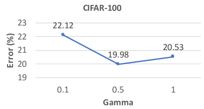
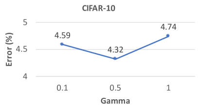
Figure 3: How errors change as $\gamma$ increases.

In Figure 3, we show how LeaSE’s classification errors on the test sets of CIFAR-10 and CIFAR-100 vary as we increase the tradeoff parameter $\gamma$. The curve on CIFAR-100 shows that the error decreases when we increase $\gamma$ from 0.1 to 0.5. The reason is that a larger $\gamma$ enables the audience to provide stronger feedback to the explainer regarding how good the explanations are. Such feedback can guide the explainer to refine its architecture for generating better explanations. However, if $\gamma$ is further increased, the error becomes worse. Under such circumstances, too much emphasis is put on evaluating how good the explanations are and less attention is paid to the predictive ability of the explainer. The architecture is biased to generating good explanations with predictive performance compromised, which leads to inferior performance. A similar trend is shown in the curve on CIFAR-10.

6 Conclusions

Motivated by humans’ explanation-driven learning skill, we develop a novel machine learning framework referred to as learning by self-explanation (LeaSE). In LeaSE, the primary goal is to help an explainer model learn how to well perform a target task. The way to achieve this goal is to let the explainer make sensible explanations. The intuition behind LeaSE is that a model has to learn to understand a topic very well before it can explain this topic clearly. A four-level optimization framework is developed to formalize LeaSE, where the learning is organized into four stages: the explainer learns a topic; the explainer explains this topic; the audience learns this topic based on the explanations given by the explainer; the explainer re-learns this topic based on the learning outcome of the audience. We apply LeaSE for neural architecture search on image classification datasets including CIFAR-100, CIFAR-10, and ImageNet. Experimental results strongly demonstrate the effectiveness of our proposed method.

References

- Alvarez-Melis and Jaakkola (2018) David Alvarez-Melis and Tommi S Jaakkola. Towards robust interpretability with self-explaining neural networks. arXiv preprint arXiv:1806.07538, 2018.
- Baehrens et al. (2010) David Baehrens, Timon Schroeter, Stefan Harmeling, Motoaki Kawanabe, Katja Hansen, and Klaus-Robert Müller. How to explain individual classification decisions. Journal of Machine Learning Research, 11(Jun):1803–1831, 2010.
- Cai et al. (2019) Han Cai, Ligeng Zhu, and Song Han. Proxylessnas: Direct neural architecture search on target task and hardware. In ICLR, 2019.
- Casale et al. (2019) Francesco Paolo Casale, Jonathan Gordon, and Nicoló Fusi. Probabilistic neural architecture search. CoRR, abs/1902.05116, 2019.
- Chen and Hsieh (2020) Xiangning Chen and Cho-Jui Hsieh. Stabilizing differentiable architecture search via perturbation-based regularization. CoRR, abs/2002.05283, 2020.
- Chen et al. (2020) Xiangning Chen, Ruochen Wang, Minhao Cheng, Xiaocheng Tang, and Cho-Jui Hsieh. Drnas: Dirichlet neural architecture search. CoRR, abs/2006.10355, 2020.
- Chen et al. (2019) Xin Chen, Lingxi Xie, Jun Wu, and Qi Tian. Progressive differentiable architecture search: Bridging the depth gap between search and evaluation. In ICCV, 2019.
- Chu et al. (2019) Xiangxiang Chu, Tianbao Zhou, Bo Zhang, and Jixiang Li. Fair DARTS: eliminating unfair advantages in differentiable architecture search. CoRR, abs/1911.12126, 2019.
- Chu et al. (2020a) Xiangxiang Chu, Xiaoxing Wang, Bo Zhang, Shun Lu, Xiaolin Wei, and Junchi Yan. DARTS-: robustly stepping out of performance collapse without indicators. CoRR, abs/2009.01027, 2020a.
- Chu et al. (2020b) Xiangxiang Chu, Bo Zhang, and Xudong Li. Noisy differentiable architecture search. CoRR, abs/2005.03566, 2020b.
- DeJong and Mooney (1986) Gerald DeJong and Raymond Mooney. Explanation-based learning: An alternative view. Machine learning, 1(2):145–176, 1986.
- Deng et al. (2009) Jia Deng, Wei Dong, Richard Socher, Li-Jia Li, Kai Li, and Li Fei-Fei. Imagenet: A large-scale hierarchical image database. In 2009 IEEE conference on computer vision and pattern recognition, pages 248–255. Ieee, 2009.
- Dong and Yang (2019) Xuanyi Dong and Yi Yang. Searching for a robust neural architecture in four GPU hours. In CVPR, 2019.
- Elton (2020) Daniel C Elton. Self-explaining ai as an alternative to interpretable ai. In International Conference on Artificial General Intelligence, pages 95–106. Springer, 2020.
- Etmann et al. (2019) Christian Etmann, Sebastian Lunz, Peter Maass, and Carola-Bibiane Schönlieb. On the connection between adversarial robustness and saliency map interpretability. arXiv preprint arXiv:1905.04172, 2019.
- Goodfellow et al. (2014) Ian J Goodfellow, Jonathon Shlens, and Christian Szegedy. Explaining and harnessing adversarial examples. arXiv preprint arXiv:1412.6572, 2014.
- He et al. (2016a) Kaiming He, Xiangyu Zhang, Shaoqing Ren, and Jian Sun. Deep residual learning for image recognition. In CVPR, 2016a.
- He et al. (2016b) Kaiming He, Xiangyu Zhang, Shaoqing Ren, and Jian Sun. Deep residual learning for image recognition. In CVPR, 2016b.
- Hong et al. (2020) Weijun Hong, Guilin Li, Weinan Zhang, Ruiming Tang, Yunhe Wang, Zhenguo Li, and Yong Yu. Dropnas: Grouped operation dropout for differentiable architecture search. In IJCAI, 2020.
- Howard et al. (2017) Andrew G. Howard, Menglong Zhu, Bo Chen, Dmitry Kalenichenko, Weijun Wang, Tobias Weyand, Marco Andreetto, and Hartwig Adam. Mobilenets: Efficient convolutional neural networks for mobile vision applications. CoRR, abs/1704.04861, 2017.
- Hu et al. (2020) Shoukang Hu, Sirui Xie, Hehui Zheng, Chunxiao Liu, Jianping Shi, Xunying Liu, and Dahua Lin. DSNAS: direct neural architecture search without parameter retraining. In CVPR, 2020.
- Huang et al. (2017) Gao Huang, Zhuang Liu, Laurens van der Maaten, and Kilian Q. Weinberger. Densely connected convolutional networks. In CVPR, 2017.
- Lei et al. (2016) Tao Lei, Regina Barzilay, and Tommi Jaakkola. Rationalizing neural predictions. Proceedings of the 2016 Conference on Empirical Methods in Natural Language Processing, 2016.
- Liang et al. (2019) Hanwen Liang, Shifeng Zhang, Jiacheng Sun, Xingqiu He, Weiran Huang, Kechen Zhuang, and Zhenguo Li. DARTS+: improved differentiable architecture search with early stopping. CoRR, abs/1909.06035, 2019.
- Liu et al. (2018a) Chenxi Liu, Barret Zoph, Maxim Neumann, Jonathon Shlens, Wei Hua, Li-Jia Li, Li Fei-Fei, Alan L. Yuille, Jonathan Huang, and Kevin Murphy. Progressive neural architecture search. In ECCV, 2018a.
- Liu et al. (2018b) Hanxiao Liu, Karen Simonyan, Oriol Vinyals, Chrisantha Fernando, and Koray Kavukcuoglu. Hierarchical representations for efficient architecture search. In ICLR, 2018b.
- Liu et al. (2019) Hanxiao Liu, Karen Simonyan, and Yiming Yang. DARTS: differentiable architecture search. In ICLR, 2019.
- Luo et al. (2018) Renqian Luo, Fei Tian, Tao Qin, Enhong Chen, and Tie-Yan Liu. Neural architecture optimization. In NeurIPS, 2018.
- Ma et al. (2018) Ningning Ma, Xiangyu Zhang, Hai-Tao Zheng, and Jian Sun. Shufflenet V2: practical guidelines for efficient CNN architecture design. In ECCV, 2018.
- Minton (1990) Steven Minton. Quantitative results concerning the utility of explanation-based learning. Artificial Intelligence, 42(2-3):363–391, 1990.
- Mullenbach et al. (2018) James Mullenbach, Sarah Wiegreffe, Jon Duke, Jimeng Sun, and Jacob Eisenstein. Explainable prediction of medical codes from clinical text. In Proceedings of the 2018 Conference of the North American Chapter of the Association for Computational Linguistics: Human Language Technologies, Volume 1 (Long Papers), pages 1101–1111, 2018.
- Noy et al. (2020) Asaf Noy, Niv Nayman, Tal Ridnik, Nadav Zamir, Sivan Doveh, Itamar Friedman, Raja Giryes, and Lihi Zelnik. ASAP: architecture search, anneal and prune. In AISTATS, 2020.
- Pham et al. (2018) Hieu Pham, Melody Y. Guan, Barret Zoph, Quoc V. Le, and Jeff Dean. Efficient neural architecture search via parameter sharing. In ICML, 2018.
- Real et al. (2019) Esteban Real, Alok Aggarwal, Yanping Huang, and Quoc V Le. Regularized evolution for image classifier architecture search. In Proceedings of the aaai conference on artificial intelligence, volume 33, pages 4780–4789, 2019.
- Ribeiro et al. (2016) Marco Tulio Ribeiro, Sameer Singh, and Carlos Guestrin. Why should i trust you?: Explaining the predictions of any classifier. In Proceedings of the 22nd ACM SIGKDD International Conference on Knowledge Discovery and Data Mining, pages 1135–1144. ACM, 2016.
- Simonyan et al. (2013) Karen Simonyan, Andrea Vedaldi, and Andrew Zisserman. Deep inside convolutional networks: Visualising image classification models and saliency maps. arXiv preprint arXiv:1312.6034, 2013.
- Smilkov et al. (2017) Daniel Smilkov, Nikhil Thorat, Been Kim, Fernanda Viégas, and Martin Wattenberg. Smoothgrad: removing noise by adding noise. arXiv preprint arXiv:1706.03825, 2017.
- Such et al. (2019) Felipe Petroski Such, Aditya Rawal, Joel Lehman, Kenneth O. Stanley, and Jeff Clune. Generative teaching networks: Accelerating neural architecture search by learning to generate synthetic training data. CoRR, abs/1912.07768, 2019.
- Szegedy et al. (2015) Christian Szegedy, Wei Liu, Yangqing Jia, Pierre Sermanet, Scott Reed, Dragomir Anguelov, Dumitru Erhan, Vincent Vanhoucke, and Andrew Rabinovich. Going deeper with convolutions. In CVPR, 2015.
- Tan et al. (2019) Mingxing Tan, Bo Chen, Ruoming Pang, Vijay Vasudevan, Mark Sandler, Andrew Howard, and Quoc V. Le. Mnasnet: Platform-aware neural architecture search for mobile. In CVPR, 2019.
- Wang et al. (2020) Xiaoxing Wang, Chao Xue, Junchi Yan, Xiaokang Yang, Yonggang Hu, and Kewei Sun. Mergenas: Merge operations into one for differentiable architecture search. In IJCAI, 2020.
- Xie et al. (2019) Sirui Xie, Hehui Zheng, Chunxiao Liu, and Liang Lin. SNAS: stochastic neural architecture search. In ICLR, 2019.
- Xu et al. (2020) Yuhui Xu, Lingxi Xie, Xiaopeng Zhang, Xin Chen, Guo-Jun Qi, Qi Tian, and Hongkai Xiong. PC-DARTS: partial channel connections for memory-efficient architecture search. In ICLR, 2020.
- Yang et al. (2016) Zichao Yang, Diyi Yang, Chris Dyer, Xiaodong He, Alex Smola, and Eduard Hovy. Hierarchical attention networks for document classification. In Proceedings of the 2016 Conference of the North American Chapter of the Association for Computational Linguistics: Human Language Technologies, pages 1480–1489, 2016.
- Zeiler and Fergus (2014) Matthew D Zeiler and Rob Fergus. Visualizing and understanding convolutional networks. In European Conference on Computer Vision, pages 818–833. Springer, 2014.
- Zela et al. (2020) Arber Zela, Thomas Elsken, Tonmoy Saikia, Yassine Marrakchi, Thomas Brox, and Frank Hutter. Understanding and robustifying differentiable architecture search. In ICLR, 2020.
- Zhang et al. (2018) Xiangyu Zhang, Xinyu Zhou, Mengxiao Lin, and Jian Sun. Shufflenet: An extremely efficient convolutional neural network for mobile devices. In CVPR, 2018.
- Zhou et al. (2019) Hongpeng Zhou, Minghao Yang, Jun Wang, and Wei Pan. Bayesnas: A bayesian approach for neural architecture search. In ICML, 2019.
- Zintgraf et al. (2017) Luisa M Zintgraf, Taco S Cohen, Tameem Adel, and Max Welling. Visualizing deep neural network decisions: Prediction difference analysis. International Conference on Learning Representations, 2017.
- Zoph and Le (2017) Barret Zoph and Quoc V. Le. Neural architecture search with reinforcement learning. In ICLR, 2017.
- Zoph et al. (2018) Barret Zoph, Vijay Vasudevan, Jonathon Shlens, and Quoc V Le. Learning transferable architectures for scalable image recognition. In CVPR, 2018.