aainstitutetext:
Departments of Physics, Keio University, 4-1-1 Hiyoshi, Kanagawa 223-8521, Japan
bbinstitutetext: KEK Theory Center, Tsukuba 305-0801, Japan††institutetext: Graduate University for Advanced Studies (Sokendai),
Tsukuba 305-0801, Japan††institutetext: RIKEN iTHEMS, RIKEN, Wako 351-0198, Japanccinstitutetext:
Theoretical Research Division, Nishina Center, RIKEN, Wako, Saitama 351-0198, Japan
Second order chiral kinetic theory under gravity and antiparallel charge-energy flow
We derive the chiral kinetic theory under the presence of a gravitational Riemann curvature.
It is well-known that in the chiral kinetic theory there inevitably appears a redundant ambiguous vector corresponding to the choice of the Lorentz frame.
We reveal that on top of this conventional frame choosing vector, higher-order quantum correction to the chiral kinetic theory brings an additional degrees of freedom to specify the distribution function.
Based on this framework, we derive new types of fermionic transport, that is, the charge current and energy-momentum tensor induced by the gravitational Riemann curvature.
Such novel phenomena arise not only under genuine gravity but also in a (pseudo-)relativistic fluid, for which inhomogeneous vorticity or temperature are effectively represented by spacetime metric tensor.
It is especially found that the charge and energy currents are antiparallelly induced by an inhomogeneous fluid vorticity (more generally, by the Ricci tensor ), as a consequence of the spin-curvature coupling.
We also briefly discuss possible applications to Weyl/Dirac semimetals and heavy-ion collision experiments.
Transport phenomena are a pivotal subject in modern quantum field theories.
Similar to external electromagnetic fields, (effective) background gravitational fields are intriguing sources to generate various currents.
First, the most widely well-known example is fluid vorticity;
the fluid velocity can be described by a metric tensor of the comoving frame with fluid.
The corresponding transport phenomenon, i.e., the chiral vortical effect (CVE) Vilenkin:1979ui can be regarded as the gravitational counterpart of the chiral magnetic effect (CME) Vilenkin:1980fu ; Nielsen:1983rb ; Fukushima:2008xe , as is clear from the gravitoelectromagnetism Landsteiner:2011cp .
The CVE is not only a theoretically interesting phenomenon in the sense that it is originated from quantum anomaly Son:2009tf ; Landsteiner:2011cp , but also an important experimental probe to study the rotation of quark-gluon plasmas created in relativistic heavy-ion collision experiments STAR:2017ckg .
Second, the mechanical strain plays a role of an effective or axial magnetic field, and accordingly yields a charge current PhysRevLett.115.177202 ; Cortijo:2016wnf ; PhysRevX.6.041046 .
Third, spacetime torsion is recently under active investigation, as it can bring novel currents, which are referred to as the chiral torsional effect Sumiyoshi:2015eda ; Khaidukov:2018oat ; Ferreiros:2018udw ; Imaki:2019ite ; Imaki:2020csc ; Gao:2020gcf .
In contrast to the aforementioned effects from the spacetime geometry, we do not fully understand the effect of the gravitational Riemann curvature in the quantum transport theory.
Even at the classical level, however, its importance has been known;
the trajectory of a spinning particle is modified by the Riemann curvature Mathisson:1937zz ; Dixon:1970zza ; Papapetrou:1951pa .
In the context of quantum transport theory, this knowledge suggests that the Riemann curvature can be the trigger of a characteristic transport of the fermion chirality (or spin, more generally).
In cosmological systems, such spacetime distortions may become dominant contributions to determine the fermionic transport rather than background electromagnetic fields.
In laboratory environments, a fluid motion and temperature gradient can be described by effective gravities leading to non-vanishing Riemann curvatures.
Therefore, the curvature-induced transport phenomena could be relevant in a wide range of physics from table-top experiments to the Universe.
For the nonequilibrium dynamics in the weak interaction regime, one of the promising theoretical implements would be the kinetic theory.
In particular, the so-called chiral kinetic theory (CKT) Stephanov:2012ki ; Son:2012wh ,
which nicely reproduces the chiral anomaly, plays a pivotal role in the development of various studies of the chiral transport phenomena Son:2012zy ; Chen:2012ca ; Manuel:2013zaa ; Chen:2014cla ; Chen:2015gta ; Hidaka:2016yjf ; Hidaka:2017auj ; Mueller:2017lzw ; Mueller:2017arw ; Huang:2018wdl ; Carignano:2018gqt ; Dayi:2018xdy ; Liu:2018xip ; Lin:2019ytz ; Carignano:2019zsh in the context of heavy-ion collision, condensed matter and neutrino physics;
although the kinetic theory is inapplicable to strongly-coupled quark-gluon plasmas, the early stage of heavy-ion collisions is described well by the Boltzmann transport theory Baym:1984np ; Mueller:1999pi ; Baier:2000sb .
The CKT conventionally involves only the leading order quantum correction so that the anomalous aspects can be taken into account as the Berry curvature.
However, the leading order CKT is insufficient to capture the gravitational curvature contributions to the transport coefficients, although the kinetic equation involves the spin-curvature coupling Liu:2018xip .
As is readily expected, higher-order corrections make the theory much more complicated, and an intuitive deduction would not avail.
This fact can be found from the equilibrium distribution function.
The contribution to enter the distribution is anticipated to be the spin-vorticity coupling, if we recall the conservation of the total angular momentum Chen:2015gta .
On the other hand, this intuition is inapplicable to the contribution, particularly, under a background gravitational field, as it is nontrivial to identify how the total angular momentum is modified at this order.
Unlike the effective formalisms that relied on the Berry curvature, the derivation from quantum field theory works well against such a complication.
In this case, the semiclassical (or weak coupling) dynamics is described by the Wigner transformation of the fermion propagator, which is a quantum-extended quantity of the classical distribution function.
The Wigner function approach systematically involves quantum corrections appearing in the CKT, and definitely keeps the covariance of the fundamental theory Hidaka:2016yjf even in the general coordinate system Liu:2018xip .
In this paper, thus we study the semiclassical transport theory with gravitational Riemann curvatures, based on the CKT derived with the Wigner function.
In the following, we present a summary of the findings in this paper.
First, we solve the collisionless CKT in general coordinate and derive the Wigner function of Weyl fermions up to .
This is a contrast to the conventional works, where only the quantum correction is taken into account.
It is intriguing that the CKT in curved spacetime is systematically solvable even with the contributions, while the electromagnetic effect is not so tamable; the theory suffers from severe infrared divergence, for which so far no correct prescription is found.
The analysis of the higher-order quantum corrections reveals new aspects of the ambiguity underlying the CKT.
It is well-known that due to degrees of freedom in terms of the Lorentz frame, the distribution function of chiral fermions cannot be uniquely determined Chen:2014cla .
As a result, a frame vector representing such an ambiguity is inevitably introduced Chen:2015gta .
From the Wigner function up to , we find that on top of the conventional frame vector, there emerges a different frame vector to define the distribution function.
These extra degrees of freedom should be irrelevant to the Wigner function and thus physical quantities, as so is the conventional one.
This is one of the guiding principles to identify an equilibrium distribution function.
Indeed we find that there is no equilibrium solution for the kinetic equation in general curved spacetime.
In other words, in general, the CKT under gravity does not reach a global equilibrium without collisions.
However, we elucidate that an equilibrium solution is admitted for several gravitational fields, such as the stationary weak one.
The remaining parts are devoted to the evaluation of physical quantities from the Wigner function that we derived before.
For instance, the charge current and energy-momentum tensor are given by the momentum integrals, as follows:
(1)
with and .
Here is the Wigner function of the right-handed Weyl fermions.
Under a static weak gravity, the part of Eq. (1) correctly reproduces the CVE.
We find that under a time-dependent gravity, the CVE totally vanishes in the dynamical limit of the background gravitational field.
Although this fact is originally derived with the diagrammatic computation Landsteiner:2013aba , our calculation is its first verification based on the CKT.
Table 1: Transport phenomena induced by general weak gravity.
The static and dynamical parts are derived in Eqs. (78) and (119), respectively.
Table 2: Transport phenomena induced by weak fluid vorticity and temperature gradient.
The static and dynamical parts are derived in Eqs. (7) and (7), respectively.
The contribution of Eq. (1) corresponds to the novel transport phenomena induced by Riemann curvatures, which is also our main finding.
They are represented as the following charge current and energy-momentum tensor:
(2)
Here and are the metric-independent coefficients determined by temperature and chemical potential for right-handed fermions .
Also and are functions of Riemann curvature , Ricci tensor and Ricci scalar .
In Table 2, we summarize the analytic forms of and .
The ‘static’ (‘dynamical’) implies that a time-independent (time-dependent) metric tensor is used.
We denote and being the Minkowski metric tensor.
It is demonstrated in Appendix D that the same charge current under a static gravity is also derived from different field-theoretical approaches.
This consistency apparently guarantees the validity of our formalism in this paper.
The fermionic system under a background fluid is a pedagogical and informative environment to demonstrate the aforementioned novel phenomena.
In general the fluid effect is translated into an effective curved spacetime described by the following metric tensor:
(3)
where is the fluctuation around the flat spacetime.
With this metric, temperature gradient and vorticity are given by
(4)
Applying Eq. (3) to and in Table 2, we get the transport phenomena induced by temperature gradient or the inhomogeneity of vorticity. The results are summarized in Table 2.
Here we define the shear tensor as with .
There are two crucial features of the novel transport phenomena induced by gravity (or equivalently inhomogeneous fluid profiles).
One is that even if the collisionless kinetic equation holds, these transport phenomena are induced, as so are the CME and CVE.
Therefore these do not generate any entropy, and thus be nondissipative.
This fact motivates us to analyze the relation of Tables 2 and 2 to the quantum anomaly, from different approaches, such as hydrodynamics.
This is an interesting open question that will be revisited in the future.
The other is the antiparallel flows of the charge current and energy current .
Tables 2 and 2 for show the coefficients of these currents have opposite signs whether the metric is static or dynamical and whatever the metric tensor is.
This is never explained by the classical particle motions; both charge and energy are carried along the classical particle momenta.
The essential ingredient of the antiparallel flow is the spin-Riemann-curvature coupling.
To find a more intuitive explanation of such curious flows is also a fascinating task.
In these respects, the novel gravity-induced transport phenomena should involve a lot of implications, e.g., in heavy-ion collisions or Dirac/Weyl semimetals (some of them are discussed in this paper).
The latter systems may provide a good playground to study our novel phenomena and can be complementary environments to the former.
For them, we need more detailed analysis based on the hydrodynamic model calculation, and quantitative comparison between theory and experiments.
Besides, the CKT in curved spacetime and the resulting curvature-induced transport phenomena could play a more crucial role under genuine gravity, although we do not discuss it in this paper.
For example, we can discuss the geodesics deviation of chiral fermions due to the spin-curvature coupling.
Such a deviation may lead to some correction to the gravitational lensing of neutrinos liebes1964gravitational .
Also, the present work could be applicable to the physics of core-collapse supernova explosions and neutron star formations Yamamoto:2015gzz .
In this direction, we need to take the collisional effects into account Hidaka:2016yjf ; Hidaka:2017auj ; Yamamoto:2020zrs , based on the Kadanoff-Baym equation in curved spacetime, which respects the diffeomorphism covariance Hohenegger:2008zk .
This paper is organized as follows.
In Sec. 2, solving the constraint equations, we obtain the general solution of the Wigner function up to under general curved spacetime.
In Sec. 3, we determine an equilibrium distribution function involving corrections, based on the frame-independence of the Wigner function.
In Sec. 4, we obtain curvature-induced charge current and energy-momentum tensor in equilibrium, which is consistent with different field-theoretical approaches in Appendix D.
In Secs. 5 and 6, we analyze the dynamical response from background gravitational fields.
As a practical application, in Sec. 7 we argue the transport phenomena in a fluid with inhomogeneous vorticity and temperature, which yields effective gravitational curvatures.
In particular, we observe the antiparallel flows of charge and energy due to an inhomogeneous vorticity (or the Ricci tensor ).
Through this paper, the convention follows from Ref. Liu:2018xip .
2 Chiral kinetic theory at
We first show the brief outline of the derivation of the CKT in the Wigner function approach.
The kinetic theory is a perturbative effective theory in the infrared momentum regime.
In quantum field theory, this perturbation is equivalent to the semiclassical truncation Elze:1986qd .
The CKT is obtained from the semiclassical expansions of the equation of motions for the Wigner functions, that is, the Wigner transformed Dyson-Schwinger equation.
The Wigner function of chiral fermions obeys three equations, which correspond to Eqs. (8)-(10) in this paper.
Two of them are the constraints to the Wigner function, and the other becomes the kinetic equation eventually.
In the classical limit, the equation for the Wigner function reduces to the Boltzmann equation (27).
The Wigner function formalism gives the quantum generalization of the classical kinetic theory.
Let us start from the Wigner function for the right-handed Weyl fermions, which is defined as Fonarev:1993ht
(5)
(6)
with , , , , and .
The above is the general relativistic extension of the one in gauge theory Elze:1986qd .
Here is called the horizontal lift;
for a function on and , the horizontal lift is represented as
(7)
where is the covariant derivative in terms of diffeomorphism and the local Lorentz transformation.
The most beneficial property of is that it commutes with both and , while does not.
Hereafter we consider the Dirac theory under an external torsionless gravitational field.
In this paper, we focus on the collisionless kinetic theory.
The Dirac equation is thus given by , which brings the dynamical equation that the Wigner function obeys.
After a long computation, the set of equations for is up to given by Liu:2018xip
(8)
(9)
(10)
where we introduce the following notations:
(11)
(12)
(13)
(14)
In the above equations, we denote , the Riemann tensor is defined as with , and the Ricci tensor is .
For left-handed Weyl fermions, similar equations are derived, but only the sign in front of is flipped, as is parity-odd.
The first equation (8) corresponds to the kinetic equation while the others (9) and (10) are constraints that
determine the functional form of .
It is worthwhile to mention that Eqs. (8)-(10) are the Ward identities in terms of the symmetries that Weyl fermions respect in a given coordinate;
the gauge symmetry, the conformal symmetry, and the Lorentz symmetry, respectively Liu:2020flb .
Let us parametrize the solution for Eqs. (9) and (10) as
In the following, we look for , and that satisfy Eqs. (17)-(25).
First, let us solve the zeroth and first-order parts.
Equations (17) and (20) imply
(26)
where is a scalar function that satisfies .
From Eq. (23), we can check that there does not appear any other term in .
Equation (8) in the zeroth order, , gives the collisionless Boltzmann equation,
(27)
Higher-order terms give quantum corrections to the Boltzmann equation.
This does not necessarily mean that itself vanishes for arbitrary .
Indeed if involves , it fulfils Eq. (28).
Therefore, the first-order correction is generally written as
(29)
Here the undetermined part satisfies so that Eq. (28) holds.
Plugging this and into Eq. (24), we obtain
(30)
We contract this with , where is a vector field independent of .
Then we get
(31)
Thus the first-order correction is given by
(32)
where we define
(33)
In the above , an arbitrary vector emerges through .
This ambiguity is related to the (local) Lorentz transformation Chen:2014cla , and thus is regarded as the spin tensor defined in the frame Chen:2015gta .
In particular, at , we have , i.e., the charge density divided by the particle energy.
In this sense, can be regarded as the quantum correction to the distribution function.
Note that the solution fulfils Eqs. (18) and (21) as long as holds.
Now we solve the second-order correction.
By plugging the above and into Eq. (19), we obtain
(34)
where the derivative operator is defined as
(35)
The general form of the second-order correction then reads
(36)
Here we again introduced the undetermined part , which satisfies .
Plugging , , and into Eq. (25), we obtain
(37)
Similarly to Eq. (30), we solve the above equation by introducing a vector (this is in general different from ), as follows:
We mention that Eq. (19) is still fulfilled for the above as long as
(43)
holds.
Indeed we can check
(44)
In the second line, we utilized
(45)
which follows from the Schouten identity:
.
Also the last line follows from , and the classical kinetic equation (8), i.e., .
We stress that Eq. (43) is a crucial constraint to , especially when we determine the equilibrium distribution function (see Sec. 3).
Eventually, the Wigner function up to is derived as
(46)
As the above is a fermion propagator, performing the momentum integration involving it we evaluate a corresponding quantity of Weyl fermions under a gravitational field.
In particular, the charge current and the symmetric energy-momentum tensor are given by
(47)
where we define , and .
Here we used the expansion of the derivative; (see Appendix C in Ref. Liu:2018xip ).
In Sec. 4, we derive the equilibrium Wigner function and show that it yields the gravity-induced parts of and .
We also demonstrate that the different approaches in Appendix D lead to the same [see Eq. (78) and Eqs. (169) and (186)].
3 Frame dependence and equilibrium
In the evaluation of physical quantities such as Eq. (47), it is necessary to identify the explicit form of .
For this purpose, the frame (i.e., and ) dependences of are a crucial concept; as shown below, we derive a constraint on the distribution function from the proper transformation law under the shift of the frames.
Combined this with the kinetic equation, we determine at equilibrium, which are utilized to evaluate equilibrium transport phenomena induced by external gravity in Sec. 4.
This section is devoted to the analysis of the frame dependence and the equilibrium solution found from it.
In the above derivation of , the frame vectors and are algebraically introduced.
It is valid to expect that the frame-dependence disappears in , which generates physical quantities.
Indeed, as is well-known in the CKT, the choice of the frame vector corresponds to the Lorentz transformation, and the frame-dependence is totally compensated in physical quantities, due to the shift of .
Hence we may plausibly require that the same is true in the CKT.
That is, we determine the transformation law of under and so that the frame dependence vanishes in .
Let us first take the Lorentz transformation in terms of , namely, and , where is the matrix representation of the local Lorentz transformation.
This transformation is equivalent to the one of the frame vector as
(48)
We also parametrize the transformation of as
(49)
Due to the Lorentz covariance of , we have
(50)
Contracting Eq. (50) with and picking up only the terms, we find
We can check that the above fulfills and Eq. (54).
In the Wigner function (46), the frame vectors and are in general chosen independently.
As long as and obey the transformation laws (51), (52), (55) and (56), however, we can always set by redefining .
Then, Eq. (46) is simplified as
(57)
where we define
(58)
The transformation laws under the change of the frames and are helpful to identify the equilibrium distribution function.
Let us first start from the classical distribution , which is defined as a function of the collisional conserved quantities:
where we use Eq. (45) and define .
Although the above relation identifies the frame-dependent part involved in at equilibrium, the frame-independent part is still undetermined.
If we set such an ambiguous part in to be zero, however, we identify
(62)
This is a plausible form in the sense that the spin-vorticity coupling term is correctly reproduced:
.
In this case, the first order Wigner function (32) is written as
(63)
This fulfills the kinetic equation at Liu:2018xip .
Subsequently, with the above and , the transformation laws (52) and (56) lead to
Here, unlike the first-order correction , we explicitly keep the frame-independent ambiguity .
Importantly, this ambiguous part should be taken into account for the realization of equilibrium, as we elaborate later.
As shown in Appendix A, inserting the above distribution functions into Eq. (42), we reduce the second-order correction part to
(66)
The frame-dependence here vanishes totally, as it should.
Plugging this into the chiral kinetic equation (8), and after a straightforward calculation in Appendix B, we finally arrive at
(67)
which is the equation to determine .
However, there is in general no solution, as is obvious from the constraint (43); cannot have terms.
In other words, the collisionless CKT has no global equilibrium solution in general background curved geometry.
We note that an equilibrium distribution function with is realized in the flat spacetime limit ; the Killing equation leads to
(68)
4 Stationary weak gravity
Although the general curved spacetime does not realize an equilibrium, there may exist a special geometry having a solution for Eq. (67).
One of the simplest cases is the stationary and weak background gravitational field, where the metric tensor is given by
(69)
In this case, the time-like Killing vector is admitted.
Then, the kinetic equation (67) is drastically reduced as
(70)
Therefore, for the metric tensor (69), we identify
(71)
Hereafter, we call with Eqs. (59), (62), (65) and (71) an equilibrium distribution function.
In this section, we focus on the geometry described by Eq. (69).
Let us evaluate the charge current and the symmetric energy-momentum tensor for the equilibrium distribution function.
We employ the classical equilibrium state described by
(72)
where is a time-like Killing vector with .
Also and are the global inverse temperature and chemical potential.
In the flat spacetime limit, the classical charge density becomes
(73)
with .
From Eq. (47), the equilibrium Wigner function yields the CVE Chen:2015gta :
(74)
where the vorticity vector is introduced as .
Here the coefficients are defined as
(75)
and thus we find and (see Appendix C).
The above charge current is conserved, namely, .
This reflects the absence of the gravitational contribution to the anomaly in the CKT up to .
Besides, the energy-momentum conservation holds, as we check .
From Eq. (66) and (71), the second order equilibrium Wigner function reads
(76)
where is the Ricci scalar.
Here we dropped the terms including because they are of order .
In the momentum integral, the terms can be rewritten as
(77)
which follows from .
The integral with is also computed in a similar manner with .
With the help of several formulas in Appendix C, we eventually derive
(78)
with .
Therefore, based on the CKT, we reveal that the nonvanishing fermion transport is induced by the background gravitational field even in equilibrium.
This implies that these phenomena are nondissipative, as so are the CME, and CVE.
This is one of the main findings of this paper.
We can also derive the same current from the diagrammatic computation (see Appendix D.1) and with the Riemann normal coordinate expansion (see Appendix D.2).
It is worthwhile to mention that enters in Eqs. (74) and (78) only through the field strength .
This is a consequence of the Kaluza-Klein gauge symmetry Banerjee:2012iz .
For the left-handed Weyl fermion, and are written as the same form, while the sign of and flipped;
the former does not involve while the latter does.
As a result, the vector and axial parts are written as
(79)
where , and , with and being the vector and chiral chemical potential, respectively.
In Sec. 7, we argue the novelty and some implications of Eq. (78) and (79).
5 Dynamical weak gravity
While so far we have focused on the equilibrium state, this section is dedicated to discuss the dynamical response from the time-dependent gravity.
Specifically, we consider a plane-wave weak background gravitational field:
(80)
where is the momentum of the gravitational field.
Let us look for the perturbative distribution function represented as the following form:
(81)
Here and are constant, and thus is the static and homogeneous solution of the collisionless Boltzmann equation (27) for .
We define as the fluctuation around .
For , we may employ the anzatz .
For simplicity, we further assume .
We first compute the classical and leading order parts.
Plugging the general form of in Eqs. (26) and (32) into Eq. (8), we write down the kinetic equation as
(82)
Expanding the above equation in terms of and utilizing , we obtain
(83)
where we denote .
Note that after the weak gravitational field expansion, all indices are raised and lowered by and the inner products are defined as and .
Especially, to get the above equation, we have taken the following replacement:
(84)
(85)
which follow from and .
For , the fluctuations are found to be
(86)
(87)
with the linearized Christoffel symbol and Riemann tensor being
(88)
Plugging the above distribution functions into Eqs. (26) and (32), we get the Wigner function.
It is here informative to decompose the Wigner function into the terms that involve the -dependent pole in the denominator, and the others.
As we show in Sec. 6, the momentum integrals of the former vanishes in the static limit , while those of the latter survives.
In this sense, we denote such a (non)static part as .
We note that the static part reproduces the equilibrium Wigner function in the previous section, as we show later.
where we use and .
Similarly, Eqs. (86) and (87) yield to the part as
(91)
where we used Eq. (45) to remove .
We again stress that while is the frame-dependent, the Wigner function is irrelevant to the frame.
Then, the Wigner function is represented as with
(92)
(93)
We observe that the above is consistent with the equilibrium Wigner function in Eq. (63).
Applying the totally same manner to the parts, we obtain and eventually the Wigner function as with
(94)
(95)
for which the precise derivation is shown in Appendix F.
Again is the same as in Eq. (66) up to .
6 Dynamical response
In the following discussion, we evaluate the charge current and the energy-momentum tensor in Eq. (47) with Eqs. (94), and (95).
As the Wigner function is decomposed into the static (-independent) and nonstatic (-dependent) part, so are and , that is, and .
The static part is calculated in the same manner as before.
For instance, using the integral formulas in Appendix C, the momentum integrals of the classical contribution (89) yield
(96)
with .
Here we use , and perform the integration by part.
For the nonstatic part, it is helpful to additionally prepare the following tensor (scalar for ) function:
(97)
where we define and the integral is over the solid angle of .
The evaluations of ’s are summarized in Appendix G.
Here in the denominators is understood to involve the positive infinitesimal imaginary part .
The nonstatic part of the classical charge current is from Eq. (90) evaluated as
(98)
To obtain the above second line, we utilized and
(99)
with and .
Besides, the nonstatic part of the classical energy-momentum tensor is computed as
(100)
It is worthwhile to notice several properties of the above .
First we find the following relations:
(101)
(102)
(103)
(104)
From these, we can show the charge current and energy-momentum conservation for arbitrary :
(105)
Second, we check that fulfills another type of relations:
(106)
(107)
(108)
These bring the dilatation current conservation for arbitrary :
(109)
As a particular case, we consider the dynamical limit .
We expand and in terms of , with the asymptotic forms of ’s, which are derived in Eqs. (215)-(219).
For later convenience, we here define the total charge current and energy-momentum tensor in the dynamical limit, as follows:
(110)
Their classical contributions hence become
(111)
Let us also calculate quantum corrections.
At , the Wigner function (93) leads to
(112)
where the vorticity is linearized as
(113)
In particular, taking the dynamical limit, we find
(114)
These results, combined with the static parts (74), yield the contributions of Eq. (110), as follows:
(115)
Therefore we conclude that the CVE vanishes in the dynamical limit.
This is consistent with the diagrammatic calculation in Ref. Landsteiner:2013aba .
At , from the Wigner function (95), the nonstatic parts are evaluated as
(116)
In the dynamical limit , we obtain
(117)
Here we used
(118)
which follow from the second Bianchi identity.
Combining these with the static contribution (78), we write the contributions of Eq. (110) as
(119)
We note that Eqs. (101)-(104) and Eqs. (106)-(108) again result in the conservation laws , and for arbitrary .
In the next section, we discuss some implications of (119) in the fluid frame [see Eq. (7)].
7 Fluid frame
The fermionic system under a background fluid is pedagogical and informative to show the novelty of the gravity-induced transport phenomena given by Eqs. (78) and (119).
In general, the effect of the fluid can be translated to that of an effective curved geometry with the following metric Banerjee:2012iz :
(120)
Adopting this metric, we represent the temperature gradient Luttinger:1964zz and the fluid vorticity as
(121)
with being the global temperature.
Alternatively, the present coordinate describes the system under the gravitoelectromagnetic fields
and .
The nonvanishing components of the curvature tensors read
(122)
with .
Inserting Eq. (122) into Eqs. (78) and (119), we readily obtain the transport phenomena under the temperature gradient and inhomogeneous vorticity.
In the static limit (or equivalently, for the stationary metric ), Eq. (78) is written explicitly as
(123)
with and .
Similarly, from the expression in the dynamical limit (119), we find
where we introduce the shear tensor:
(125)
The corresponding vector and axial-vector currents are obtained by replacing with , and with and respectively, as we have done to get Eq. (79).
Several comments are in order.
We again emphasize that Eq. (7) represents equilibrium transport phenomena, like the CME and CVE.
It is also intriguing to notice the difference between these and Fourier’s law.
For the former, the currents in Eq. (7) come from the vorticity, namely, the magnetic part of the gravity.
This background source supplies no energy to particles, and thus the currents become finite even in equilibrium.
On the other hand, the latter is the current generation by the temperature gradient.
This electric part of the gravitational field gives an energy to particles.
Therefore the Fourier’s law is dissipative and prohibited in equilibrium.
For an static and spatially inhomogeneous vorticity , there emerges the nonvanishing charge current and the energy current , on top of the contributions from the CVE (74).
Unlike the vector part of the CVE, the curvature-induced currents (79) or (7) does not require .
In the system without the chiral imbalance, hence, and are the leading vortical contributions.
In the dynamical limit, such second-order contributions become more important, since the CVE is washed out as shown in Eq. (115) while the currents in Eq. (7) are not.
Under the correspondence between magnetic field and vorticity, one would think that the charge current is the gravitational analogue of Ampère’s law: .
The situation is however not so trivial since is opposite-signed against the energy current (for ).
Namely, Eqs. (7) and (7) cannot be explained based on the naive picture that a particle’s momentum carries both charge and energy.
This curious flow dynamics essentially comes from the quantum effects through the spin-curvature coupling.
We should emphasize that such an antiparallel charge-energy flow is not restricted in the present coordinate, but more generally admitted in a lot of curved spacetime;
this phenomenon always takes place as long as , as shown in Eqs. (78) and (119).
It is worthwhile to mention the feedback to the gravitational field from Eq. (78).
In our sign convention, the Einstein field equation is given by with the gravitational constant birrell1984quantum .
Following this, the induced Ricci tensor reads with a positive coefficient .
Hence, the initial gravitational field is enhanced, which evokes the possibility of instability.
We will revisit and analyze more precisely the above brief argument in the future, including the existence of a novel collective dynamics Akamatsu:2013pjd in a gravitational plasma Nachbagauer:1995wn ; deAlmeida:1993wy .
One might think that Eq. (7) is unrelated to an anomaly.
Indeed, Eq. (7) would be irrelevant to the chiral anomaly, according to the analysis of discrete symmetry Kharzeev:2011ds .
Nevertheless, this fact is not sufficient to conclude the irrelevance to anomaly at all, as for the temperature dependent part of the CVE Golkar:2012kb ; Golkar:2015oxw ; Chowdhury:2016cmh ; Glorioso:2017lcn .
We also mention that the transport coefficients and are time-reversal even quantities, which could be associated with their nondissipative nature similarly to those of the CME and CVE Kharzeev:2011ds .
It should be required to clarify the anomalous aspect of Eq. (7) from different approaches, such as hydrodynamics.
In the sense that they are of the higher-order of the derivative counting, usual hydrodynamics can neglect Eqs. (7) and (7).
This would not be the case, however, if these phenomena originate from quantum anomaly like the CME and CVE.
These novel contributions (7) lead to several implications in relativistic many-body systems where an inhomogeneous fluid vorticity is experimentally generated.
In rotating quark-gluon plasma, there emerges the quadrupole configuration of the vorticity along the beam direction Adam:2019srw ; Becattini:2017gcx ; Wei:2018zfb ; Fu:2020oxj .
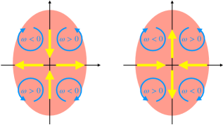
Thus, on the transverse plane to the beam direction, the inhomogeneous vorticities generate the charge current and the energy current , as depicted in Fig. 1.
As a brief argument, we may estimate the scale of the vorticity gradient to be the inverse of the hot matter size.
Indeed, at the collision energy , the gradient of the vorticity is estimated to be Wei:2018zfb .
Although the whole magnitudes of and are dependent on the scale of , hence, these are nonnegligible compared with the CVE.
Figure 1: Flow directions of (left) and (right).
The horizontal axis corresponds to the reaction plane of heavy-ion collisions.
The quadrupole vorticity structure is based on the measurement by STAR collaboration Adam:2019srw
On top of the charge and energy currents, the stress tensor is also induced.
Let us consider a cylindrical system along the direction with a spatially inhomogeneous temperature .
From the vector part of the energy-momentum tensor in Eq. (7), the temperature gradient yields the correction to the transverse pressure .
When the temperature takes a Gaussian form , we get , which has the minima and maxima .
Such a pressure correction is detectable in Weyl/Dirac semimetal experiments, similarly to the usual thermoelectric transport phenomena Lundgren:2014hra ; liang2017anomalous .
In table-top experiments, an inhomogeneous and dynamical vorticity can be generated by an acoustic surface wave.
We consider a transverse wave propagating on the surface 9780750626330 ; PhysRevLett.119.077202 ; PhysRevB.87.180402 of Weyl/Dirac semimetals.
Also we prepare the wave propagating along the direction, and its amplitude is normal to the surface, i.e., its displacement vector is given by with .
Here reflects unpenetrating into the material.
Now the response to this surface wave can be evaluated in the coordinate space described by with , , and other components of vanishing.
From Eq. (7) together with the Wick rotation ,
we get the charge and energy currents: , and , .
The flows normal to the fluid velocity are induced by the gravitational curvature via quantum effects.
We note that the flows parallel to the fluid velocity are induced from classical contributions.
Acknowledgements.
This work was supported by JSPS KAKENHI Grant Numbers 17H06462 and 18H01211.
K. M. was supported by Special Postdoctoral Researcher (SPDR) Program of RIKEN.
In this appendix, we show the concrete expression of at equilibrium defined by Eqs. (59), (62), (65) and (71).
We decompose in Eq. (42) into the frame-(in)dependent and the part:
(126)
The first term reads
(127)
The frame-dependent part is further decomposed as
(128)
where we define
(129)
For the equilibrium distribution in Eq. (59), we reduce and to
(130)
and
(131)
where the term is dropped, and we utilize and Eq. (45).
The frame-dependent part hence becomes
(132)
In the above equation, the frame dependence totally vanishes, as it should.
Eventually, is written as Eq. (66).
Here, we present several Integration formulas.
We first define
(143)
In particular, the first four ’s are
(144)
(145)
(146)
(147)
Also in the integral of angular degrees of freedom, we can replace the product of ’s in the integral, as follows:
(148)
where and .
Appendix D Alternative derivation of
In this appendix, we derive the curvature-induced charge current in Eq. (78), from the thermodynamics of Weyl fermions in a curved spacetime.
At the same time, such alternative derivations leading to the same ensures the correctness of the Wigner function in Eq. (46) and the equilibrium distribution function given by Eqs. (65) and (71).
D.1 Diagrammatic computation
First, we derive the current of a chiral fluid under a gravitational field, based on the linear response theory.
We consider a Weyl fermion, and the corresponding action is given by
(149)
where we introduce with the Pauli matrices
.
Here denotes (inverse) vierbein satisfying
with the spacetime curved metric and Minkowski metric
, and .
The left and right covariant derivatives are defined as
(150)
with , which satisfies
.
Furthermore, employing the torsionless condition,
we can express the spin connection
as
(151)
The energy-momentum tensor and covariant charge current are
defined as
(152)
Note that is not symmetric, so we introduce the symmetric energy-momentum tensor defined as .
In the following, we consider fluctuation around the flat metric .
In the linear response theory, the current in momentum space can be expressed as
(153)
with
(154)
where we define and denotes the imaginary time ordering.
The two point correlator is computed with the Feynman rule in flat spacetime:
(155)
(156)
(157)
In momentum space, at one-loop order, we get
(158)
where we denote , and , and the antisymmetric tensor is normalized as .
Also we introduced
(159)
In order to compute the liner response to the gravitational field, we expand in terms of and define to be the contribution of .
In particular, we find
(160)
There are two steps to compute the momentum integrals.
First, the radial integral is systematically evaluated with the following formulas:
(161)
(162)
with
(163)
(164)
The above formulas are proved in Appendix E.
Second, for the angle integrals in Eq. (160), we replace the momentum products , as shown in Eq. (148).
Then we obtain
(165)
where we denote .
As a result, the contribution in Eq. (158) is written as
(166)
which reproduces the CVE:
(167)
with .
Similarly, the parts are computed as
(168)
For the stationary gravitational field (), we eventually derive
We reproduce the fermionic current in Eq. (78), by employing the Riemann normal coordinate (RNC) expansion parker2009quantum .
We first look for the propagator that satisfies
(171)
where we denote and .
Here is the diffeomorphic and local Lorentz covariant derivative with respect to , and the spin connection is defined as
(172)
Further we introduce the following bispinor (not scalar) propagator:
Let us now introduce the RNC.
We define the normal coordinate and the origin is at , that is, we replace and .
In order to evaluate above Green’s function, we perform the RNC expansion, as follows:
(175)
(176)
(177)
(178)
(179)
where denotes the or contribution.
Note that all of the above curvature tensors are evaluated at .
We thus reduce Eq. (174), as follows:
(180)
Now we perform the Fourier transformation:
(181)
with .
Then obeys
(182)
where we denote and is the derivative operators of .
The above equation is solved sequentially, as follows:
(183)
Thus we obtain
(184)
Performing the Wick rotation, we obtain the vector current as
(185)
with .
The above current is evaluated with Eq. (148).
The first term in the above integrand gives the ordinary charge density.
The other terms are linear in the curvature tensor, and thus the curvature-induced current is calculated as
(186)
This is again the same as Eq. (78) up to the factor , which comes from the right- and left-handed contributions.
Appendix E Evaluation of and
In this appendix, we derive the formulas of the momentum integrals in Euclidean spacetime, which are applied in Appendix D.
We first compute the following integral:
(187)
This obeys the recursion relation , and the solutions are given by
(188)
We calculate as
(189)
Therefore, we obtain
(190)
One can check that this solution satisfies the recursion relation:
which obeys the same recursion relation .
In the same manner for , we get
(194)
(195)
(196)
The overall factor is calculated as
(197)
Here, (const) denotes the divergent term that is independent of and .
Appendix F Wigner function under the dynamical gravity (94) and (95)
In this appendix, we derive the Wigner function under a time-dependent gravitational field, Eqs. (94) and (95).
Plugging and given by Eqs. (46) and (11), we write down the kinetic equation (8) as
(198)
Here and involved in have already been obtained in Eqs. (86) and (87).
After some computation keeping together with and , we reduce the kinetic equation (198) to
(199)
which yields the second order fluctuation as
(200)
Collecting Eqs. (86) and (87), the above and the general form of the Wigner function (42), we find
(201)
In the above equation, there are the four frame-dependent terms.
However, the dependence is totally cancelled out, as shown in the following.
These are rewritten as
(202)
(203)
(204)
(205)
where we use Eq. (45), and the second Bianchi identity (133) for .
Hence, the four frame-dependent terms in Eq. (LABEL:eq:Rmu2_dyn_app) are recast into
(206)
Inserting this into Eq. (LABEL:eq:Rmu2_dyn_app), we finally derive Eqs. (94) and (95).
Appendix G Angle integrals
In this appendix, we derive the integral formulas in terms of the momentum angle valuables.
We introduce the following function for the angular integral:
(207)
where involves the positive infinitesimal imaginary part and we define .
By definition, we can readily show Eqs. (101)-(104) and Eqs. (106)-(108).
Let us now evaluate the angle integrals.
We define and as the polar and azimuthal angles when the polar axis is along .
First, we compute
(208)
with .
In order to evaluate the other integrals, we prepare the following formulas:
(209)
where we introduce (we note ).
We prepare the following integrals:
(210)
These yield
(211)
(212)
(213)
(214)
In particular, the asymptotic forms of in the dynamical limit are
(215)
(216)
(217)
(218)
(219)
On the other hand, in the static limit , we find .
References
(1)
A. Vilenkin, MACROSCOPIC PARITY VIOLATING EFFECTS: NEUTRINO FLUXES FROM
ROTATING BLACK HOLES AND IN ROTATING THERMAL RADIATION,
Phys. Rev.D20 (1979) 1807.
(2)
A. Vilenkin, EQUILIBRIUM PARITY VIOLATING CURRENT IN A MAGNETIC FIELD,
Phys. Rev.D22 (1980) 3080.
(3)
H.B. Nielsen and M. Ninomiya, ADLER-BELL-JACKIW ANOMALY AND WEYL
FERMIONS IN CRYSTAL,
Phys. Lett.130B (1983) 389.
(7)STAR collaboration, Global hyperon polarization in
nuclear collisions: evidence for the most vortical fluid,
Nature548
(2017) 62 [1701.06657].
(8)
A. Cortijo, Y. Ferreirós, K. Landsteiner and M.A.H. Vozmediano, Elastic
gauge fields in weyl semimetals,
Phys. Rev. Lett.115 (2015) 177202.
(9)
A. Cortijo, D. Kharzeev, K. Landsteiner and M.A.H. Vozmediano, Strain
induced Chiral Magnetic Effect in Weyl semimetals,
Phys. Rev.B94 (2016) 241405
[1607.03491].
(10)
A.G. Grushin, J.W.F. Venderbos, A. Vishwanath and R. Ilan, Inhomogeneous
weyl and dirac semimetals: Transport in axial magnetic fields and fermi arc
surface states from pseudo-landau levels,
Phys. Rev. X6 (2016) 041046.
(23)
J.-W. Chen, S. Pu, Q. Wang and X.-N. Wang, Berry Curvature and
Four-Dimensional Monopoles in the Relativistic Chiral Kinetic Equation,
Phys. Rev. Lett.110 (2013) 262301
[1210.8312].
(24)
C. Manuel and J.M. Torres-Rincon, Kinetic theory of chiral relativistic
plasmas and energy density of their gauge collective excitations,
Phys. Rev. D89 (2014) 096002
[1312.1158].
(29)
N. Mueller and R. Venugopalan, The chiral anomaly, Berry’s phase and
chiral kinetic theory, from world-lines in quantum field theory,
Phys. Rev. D97 (2018) 051901
[1701.03331].
(31)
A. Huang, S. Shi, Y. Jiang, J. Liao and P. Zhuang, Complete and
Consistent Chiral Transport from Wigner Function Formalism,
Phys. Rev.D98 (2018) 036010
[1801.03640].
(32)
S. Carignano, C. Manuel and J.M. Torres-Rincon, Consistent relativistic
chiral kinetic theory: A derivation from on-shell effective field theory,
Phys. Rev.D98 (2018) 076005
[1806.01684].
(33)
O.F. Dayi and E. Kilin@ c@ carslan, Quantum Kinetic Equation in the
Rotating Frame and Chiral Kinetic Theory,
Phys. Rev. D98 (2018) 081701
[1807.05912].
(35)
S. Lin and A. Shukla, Chiral Kinetic Theory from Effective Field Theory
Revisited, JHEP06 (2019) 060
[1901.01528].
(36)
S. Carignano, C. Manuel and J.M. Torres-Rincon, Chiral kinetic theory
from the on-shell effective field theory: Derivation of collision terms,
Phys. Rev. D102 (2020) 016003
[1908.00561].
(37)
G. Baym, THERMAL EQUILIBRATION IN ULTRARELATIVISTIC HEAVY ION
COLLISIONS, Phys.
Lett. B138 (1984) 18.
(41)
S. Liebes Jr, Gravitational lenses, Physical Review133 (1964) B835.
(42)
N. Yamamoto, Chiral transport of neutrinos in supernovae:
Neutrino-induced fluid helicity and helical plasma instability,
Phys. Rev.D93 (2016) 065017
[1511.00933].
(44)
A. Hohenegger, A. Kartavtsev and M. Lindner, Deriving Boltzmann
Equations from Kadanoff-Baym Equations in Curved Space-Time,
Phys. Rev. D78 (2008) 085027
[0807.4551].
(45)
H.T. Elze, M. Gyulassy and D. Vasak, Transport Equations for the QCD
Quark Wigner Operator,
Nucl. Phys.B276 (1986) 706.
(48)
N. Banerjee, J. Bhattacharya, S. Bhattacharyya, S. Jain, S. Minwalla and
T. Sharma, Constraints on Fluid Dynamics from Equilibrium Partition
Functions, JHEP09 (2012) 046 [1203.3544].
(54)
D.E. Kharzeev and H.-U. Yee, Anomalies and time reversal invariance in
relativistic hydrodynamics: the second order and higher dimensional
formulations, Phys.
Rev. D84 (2011) 045025
[1105.6360].
(55)
S. Golkar and D.T. Son, (Non)-renormalization of the chiral vortical
effect coefficient,
JHEP02
(2015) 169 [1207.5806].
(60)
F. Becattini and I. Karpenko, Collective Longitudinal Polarization in
Relativistic Heavy-Ion Collisions at Very High Energy,
Phys. Rev. Lett.120 (2018) 012302
[1707.07984].
(64)
T. Liang, J. Lin, Q. Gibson, T. Gao, M. Hirschberger, M. Liu et al.,
Anomalous nernst effect in the dirac semimetal cd 3 as 2,
Physical review letters118 (2017) 136601.
(65)
L.D. Landau and E.M. Lifshitz, Theory of Elasticity,
Butterworth-Heinemann, Oxford, 3 ed. (1986).
(66)
D. Kobayashi, T. Yoshikawa, M. Matsuo, R. Iguchi, S. Maekawa, E. Saitoh et al.,
Spin current generation using a surface acoustic wave generated via
spin-rotation coupling,
Phys. Rev. Lett.119 (2017) 077202.
(67)
M. Matsuo, J. Ieda, K. Harii, E. Saitoh and S. Maekawa, Mechanical
generation of spin current by spin-rotation coupling,
Phys. Rev. B87 (2013) 180402(R)
[1301.3596].
(68)
L. Parker and D. Toms, Quantum field theory in curved spacetime:
quantized fields and gravity, Cambridge University Press (2009).