Shaping the Transient Response of Nonlinear Systems
to Satisfy a Class of Integral Constraints

Abstract

We consider the problem of shaping the transient step response of nonlinear systems to satisfy a class of integral constraints. Such constraints are inherent in hybrid energy systems consisting of energy sources and storage elements. While typical transient specifications aim to minimize overshoot, this problem is unique in that it requires the presence of an appreciable overshoot to satisfy the foregoing constraints. The problem was previously studied in the context of stable linear systems. A combined integral and feedforward control, that requires minimal knowledge of the plant model, was shown to make the system amenable to meeting such constraints. This paper extends that work to nonlinear systems and proves the effectiveness of the same compensation structure under added conditions. Broadly, it is shown that the integral constraint is satisfied when this compensation structure is applied to nonlinear systems with stable open-loop step response and a positive DC gain. However, stability of the resulting closed-loop system mandates bounds on the controller gain.

1 Introduction

In many control systems, having a desired transient response is one of the main objectives. In particular, time domain specifications, control signal magnitude, controller complexity, overshoots/ undershoots and satisfying predefined constraints, are important considerations in transient characteristics, [1]. The studies [2, 3] are among the first works on the transient response of rational transfer functions.

Different approaches to shape transient response through compensator design appear in [4, 5, 6]. Feedforward techniques have also been proposed to shape the transient response of linear systems for the cases of tracking an input reference. These techniques include inversion-based feedforward, [7, 5]. In the presence of parametric uncertainties, these methods violate the imposed constraints and can result in deterioration of performance, [8]. Another issue with the inversion-based feedforward compensation is that not all of the zeros are cancellable, for instance for non-minimum phase systems, a remedy for which is discussed in [9]. Inserting additional zeros in the feedforward path for reducing the tracking errors is investigated in [10].

To improve the transient response of a servosystem obtained in a mode switching control, [11] proposes a method of giving an additional input in the form of an impulse response. Specific transient characteristics, such as the number of extrema in step responses are studied in [12]. In [13], the open-loop nature of input shaping is considered for vibration control of flexible systems, in the presence of known and finite duration disturbances. Input shaping has been extensively used for vibration control (see [14] and references therein). Transient response of nonlinear systems is addressed in fewer works in the literature, with some examples being [15, 16]. Constraints imposed on transient response are soft or hard. Soft constraints are similar to imposing a desirable second order performance on the controlled system, and hard constraints can be maintaining the output limited in a specific narrow range, [1]. Model predictive control is one of the approaches to handle hard constraints, [17]. This paper, like most works referenced above, deals with soft constraints.

In this paper, we study the problem of satisfying a class of integral constraints imposed on the step response of nonlinear systems. The problem is relevant in hybrid power systems where power resources and Energy Storage Systems (ESSs) are combined. For instance, in hybrid fuel cell and ultra-capacitor systems, load-following ability is directly correlated to satisfying these constraints. The load following mode for hybrid energy systems is discussed in [18, 19]. In this mode, the ESS provides or absorbs power immediately following an abrupt fluctuation in power demand, while the power source follows the load more gradually. Concurrently, a combined feedback and feedforward compensation guarantees that the ESS’s State-Of-Charge (SOC) is maintained within safe limits. Fundamentally, this SOC control translates to satisfying the integral constraints mentioned above. In [20, 21], the compensation was studied in the context of linear systems and the concept of Integral Controllability, [22, 21], was revisited. In this paper, we extend the work in [21] to nonlinear systems. We consider nonlinear systems that provide a stable step response at a fixed DC gain and derive conditions under which the compensated nonlinear system satisfies a desired integral constraint.

The rest of the paper is organized as follows; In Section 2, the constraints are explained, the viability of the aforementioned compensation structure is established for nonlinear systems and an example is given. Next, stability analysis of the compensated system is conducted in Section 3, for first order plants. In Section 4, the analysis is extended to higher order nonlinear plants and an example is provided. Subsequently concluding remarks are made and references are listed.

2 Problem Definition and Extension to Nonlinear Systems

As discussed in the Introduction, transient responses are of importance in engineering applications such as hybrid energy systems. The problem of shaping the transient step response of a linear system to satisfy an additional integral constraint was addressed in [21]. In this paper, we extend the problem to nonlinear systems. An illustration of the transient response is shown in Fig. 1. In this figure, $r$ is a step input and $y$ is the response of a dynamical system having a unity DC gain.

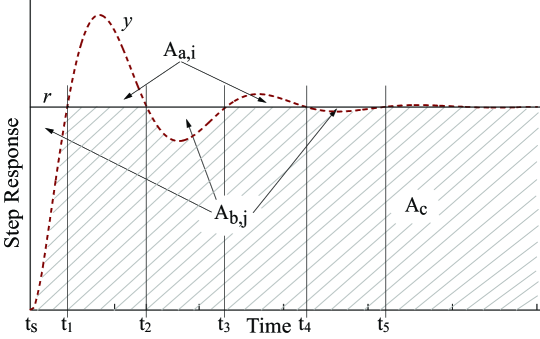
Figure 1: Transient step response with areas defining the integral constraint

There exist three different types of areas shown in Fig. 1, namely $A_{a,i}$, $A_{b,j}$, and $A_{c}$. The areas $A_{a,i}$ are located above the step input $r$ and below the response $y$. The areas $A_{b,j}$ are confined below $r$ and above $y$. $A_{c}$ refers to the common and shaded area below both $r$ and $y$. Considering these three categories, we can define

$$A_{a}=-\frac{1}{2}\int_{t_{s}}^{\infty}\Bigl{\{}1-\operatorname{sign}(r-y)\Bigr{\}}(r-y)dt\quad\Rightarrow\quad A_{a}=\sum_{i=1}^{\infty}A_{a,i},$$

$$A_{b}=\frac{1}{2}\int_{t_{s}}^{\infty}\Bigl{\{}1+\operatorname{sign}(r-y)\Bigr{\}}(r-y)dt\quad\Rightarrow\quad A_{b}=\sum_{j=1}^{\infty}A_{b,j}$$

and,

$$A_{c}=\frac{1}{2}\int_{t_{s}}^{\infty}\Bigl{\{}1-\operatorname{sign}(r-y)\Bigr{\}}r\,dt+\frac{1}{2}\int_{t_{s}}^{\infty}\Bigl{\{}1+\operatorname{sign}(r-y)\Bigr{\}}y\,dt$$

We can verify that

$$\int_{t_{s}}^{\infty}y\,dt=A_{a}+A_{c},\quad\int_{t_{s}}^{\infty}r\,dt=A_{b}+A_{c}.$$

The goal of this paper is to shape the transient step response $y$ to satisfy the integral constraint $A_{b}=A_{a}$. Such a constraint finds application in hybrid energy systems. To exemplify a practical scenario, let us assume a hybrid power system consisting of a power source and a storage unit. At an instant, if load demand increases, then the storage unit provides the extra power until the source adapts to the new power level following a transient response. In the context of Fig. 1, consider the step input $r$ to represent a sudden change in power demand and $y$ to represent the response of the power source. The contribution of the storage unit can be visualized as the difference $(r-y)$. Thus, following a sudden change in demand, the storage unit provides a surge in power while the source ramps its power supply gradually. To compensate for an excess charge/discharge accrued by the storage unit during the transient, and to satisfy the load demand simultaneously, the output $y$ needs to attain $r$ at steady state while satisfying the integral constraint $A_{b}=A_{a}$ over its transient. In this case, we have from above,

$$A_{a}=A_{b}\Rightarrow\int_{t_{s}}^{\infty}y\,dt=\int_{t_{s}}^{\infty}r\,dt\Rightarrow\int_{t_{s}}^{\infty}e\,dt=0\Rightarrow e_{r}=0$$ (1)

where, we define $e=r-y$, and $e_{r}=\int_{t_{s}}^{\infty}e\,dt$. Additionally, practical considerations such as energy losses require that the transient response can also satisfy the following integral constraints

$$A_{a}>A_{b}\Rightarrow\int_{t_{s}}^{\infty}y\,dt>\int_{t_{s}}^{\infty}r\,dt\Rightarrow\int_{t_{s}}^{\infty}e\,dt<0\Rightarrow e_{r}<0,\;\mbox{and similarly}\;A_{a}<A_{b}\Rightarrow e_{r}>0$$ (2)

In this regard, it was shown in [21] that for linear systems, by utilizing the compensation structure of Fig. 2 and using $\alpha$ as the inverse DC gain of the plant, the compensated system tracks any step input while satisfying the integral constraint of Eq. 1. Further, by varying $\alpha$ the constraints of Eq. 2 can be satisfied. In this study, we consider the plant to have nonlinear dynamics, thereby admitting more realistic models of power systems.

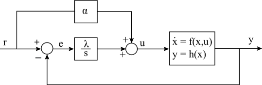
Figure 2: Compensation structure

We next prove that the compensation shown in Fig. 2 also satisfies the integral constraint for nonlinear systems under certain conditions. In this context, we consider the following nonlinear system as the original open-loop nonlinear system to evaluate the compensation strategy depicted in Fig. 2 for,

$$\dot{x}=f(x,u),\quad y=h(x)$$ (3)

where $x\in R^{n}$ is the state, $u\in R$ is the input, $y\in R$ is the output. In the closed-loop system shown in Fig. 2, $r$ is a step input and $\lambda\in R$ is a positive scalar. The system equations are as follows,

$$\dot{x}=f(x,u),\quad u=\alpha r+\lambda\int_{t_{s}}^{t}e(\tau)d\tau,\quad e=r-y,\quad t\geq t_{s}$$ (4)

We now state and prove the following lemma:

Lemma 1.

Assume Eq. 3 has a unique and asymptotically stable equilibrium point $x_{u}$, for a step input $u$. In addition, when $x=x_{u}$, let $y=h(x_{u})=u/k$, where $1/k\in R^{+}$ is the DC gain of Eq. 3. Then, the equilibrium point of the closed-loop system illustrated in Fig. 2, with the dynamic of Eq. 4 and $\lambda>0$, has the following properties,

$$y=\frac{u}{k}=r,\quad\mbox{and}\quad\int_{t_{s}}^{\infty}e(\tau)d\tau=r\left(\frac{k-\alpha}{\lambda}\right)$$ (5)

Proof.

Considering the closed-loop system depicted in Fig. 2 and Eq. 4, the state space equations of the closed-loop system are

$$\dot{x}=f(x,u),\quad\dot{u}=\lambda(r-y)$$ (6)

At equilibrium $\dot{u}=0$, implying $y=r$. Then, per the assumption in Eq. 5, Eq. 4 has a unique equilibrium point at $x=x_{u}$ and $y=u/k$. Therefore, at steady-state, we have $y=u/k=r$ and hence from Eq. 4, $\int_{t_{s}}^{\infty}e(\tau)d\tau=(u-\alpha r)/\lambda=r(k-\alpha)/\lambda$. ∎

It is noted that in open-loop, i.e. when $\lambda=0$, then $\int_{t_{s}}^{\infty}e(\tau)d\tau$ can only be determined through direct integration, as Eq. 5 is not applicable. The constraints of Eqs. 1 and 2 are satisfied by different values of $\alpha$. The assumption of uniqueness of the equilibrium $x=x_{u}$ and $y=h(x_{u})=u/k$ in Eq. 5 is not restrictive. This is because there are many practical systems that are capable of tracking step inputs either naturally or through a built-in controller, such as the energy systems considered in [21]. The goal of this work is to design a compensation for such systems so that their transient response is shaped to satisfy the integral constraints described above. While Eq. 5 describes the steady-state property of the compensated system in Fig. 2, its stability is affected by the added integral action. This stability analysis is carried out in Sections 3 and 4. We next provide an example to demonstrate the result of Eq. 5.

2.1 Example

We consider the following nonlinear system to demonstrate the concept discussed above

$$\dot{x}=-20(x-u)^{3},\quad y=x$$

The above system has a unique asymptotically stable equilibrium at $x=u$ (i.e. $k=1/\mbox{DC gain}=1$) for a step input in $u$. When placed in the compensation structure of Fig. 2 with $\lambda=8$, the responses obtained for different values of $\alpha$ are shown in Fig. 3.

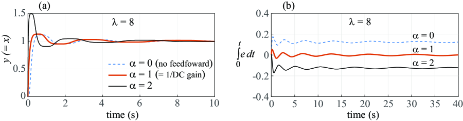
Figure 3: Illustrative example of Section 2.1

Figure 3(a) shows the step response and Fig. 3(b) shows $e_{r}=\int_{0}^{t}e(\tau)d\tau$. While in all cases $y$ tracks the step input in $r$, the choice $\alpha=1(=k)$ ensures $e_{r}=0$, and $\alpha=0$ and $2$ yield $e_{r}>0$ and $<0$ respectively.

3 Stability Analysis: First Order Nonlinear System

In this section, we conduct the stability analysis for the case where the original system has a first order nonlinear dynamics. The analysis will be extended to higher order nonlinear systems in Section 4. Without loss of generality, we assume $\alpha=1$ in Fig. 2 and state the following theorem,

Theorem 1.

Let the nonlinear open-loop system in Eq. 3 with $y=h(x)=x$ be globally exponentially stable at its unique equilibrium point $x_{u}=u$, when $u$ is a step input. Then, the closed-loop system of Eq. 6, which represents Fig. 2, has a globally exponentially stable equilibrium at $[x\,\,\,u]=[r\,\,\,r]$, for sufficiently small $\lambda>0$.

Proof.

For the open-loop first order nonlinear system, we transfer the equilibrium of Eq. 3 to the origin by defining $\bar{e}=u-x$. Considering a step input $u$, we have

$$\dot{\bar{e}}=-f(u-\bar{e},u)+\dot{u}=\bar{f}(\bar{e},u)$$ (7)

Per the assumption in Theorem 1, the origin $\bar{e}=0$ is a globally exponentially stable equilibrium in Eq. 7. Hence, using Converse Lyapunov Theorem in [23], there exists a Lyapunov function $V(\bar{e})$ such that,

$$c_{1}|\bar{e}|^{2}\leq V(\bar{e})\leq c_{2}|\bar{e}|^{2}$$ (8a)

$$\frac{\partial V}{\partial\bar{e}}\bar{f}(\bar{e},u)\leq-c_{3}|\bar{e}|^{2}$$ (8b)

$$\left|\frac{\partial V}{\partial\bar{e}}\right|\leq c_{4}|\bar{e}|$$ (8c)

where, $c_{1},\,c_{2},\,c_{3},\,c_{4}>0$. We note that $V=V(\bar{e})$ (i.e. $V$ has no dependence on $u$) is not restrictive and can be defined for many non-autonomous systems, such as the ones to be discussed in Section 3.1. When the system of Eq. 3 is compensated as shown in Fig. 2, $r$ is the step input and $\dot{u}\neq 0$. Hence, the dynamic of $\bar{e}$ takes the form, $\dot{\bar{e}}=-f(u-\bar{e},u)+\dot{u}=\bar{f}(\bar{e},u)+\dot{u}$. Additionally, per Eq. 4, $e=r-x$, thus $\dot{e}=-\dot{x}$. Hence, from Eq. 6, we have the following closed-loop equation,

$$\dot{\bar{e}}=-f(u-\bar{e},u)+\dot{u}=\bar{f}(\bar{e},u)+\dot{u}$$ (9a)

$$\dot{u}=\lambda e$$ (9b)

To prove the stability of Eq. 9, the following positive definite function $\bar{V}(\bar{e},e)$ is chosen

$$\bar{V}(\bar{e},e)=V(\bar{e})+\frac{1}{2}(u-r)^{2}=V(\bar{e})+\frac{1}{2}(\bar{e}-e)^{2}$$ (10)

In Eq. 10, we note that $u-r=u-x+x-r=\bar{e}-e$. The derivative of $\bar{V}(\bar{e},e)$ along the trajectories of Eq. 9 is

$$\dot{\bar{V}}=\frac{\partial V}{\partial\bar{e}}\dot{\bar{e}}+(u-r)(\dot{u}-\dot{r})=\frac{\partial V}{\partial\bar{e}}\left[\bar{f}(\bar{e},u)+\dot{u}\right]+\lambda e(\bar{e}-e)$$

Then,

$$\dot{\bar{V}}=\frac{\partial V}{\partial\bar{e}}\bar{f}(\bar{e},u)+\frac{\partial V}{\partial\bar{e}}\dot{u}+\lambda e(\bar{e}-e)$$

Therefore, from Eqs. 8b and 8c,

$$\dot{\bar{V}}\leq-c_{3}|\bar{e}|^{2}-\lambda|e|^{2}+\lambda(1+c_{4})|e||\bar{e}|$$ (11)

We can express Eq. 11 as

$$\dot{\bar{V}}=-\left[\begin{array}[]{cccc}\bar{e}&e\end{array}\right]\left[\begin{array}[]{cc}c_{3}&\frac{\lambda(1+c_{4})}{2}\\ \frac{\lambda(1+c_{4})}{2}&\lambda\end{array}\right]\left[\begin{array}[]{cccc}\bar{e}\\ e\end{array}\right]=-E^{T}\,Q\,E,\quad E=\left[\bar{e}\quad e\right]^{T}$$ (12)

By choosing $0<\lambda<4c_{3}/(1+c_{4})^{2}$, $Q$ becomes positive definite. Let $p_{min}$ and $p_{max}$ be the minimum and maximum eigenvalues of $Q$, respectively. Also, it can be shown from Eqs. 8a and 10 that $\bar{V}<(c_{2}+1)\lVert E\rVert^{2}$. Thus,

$$\dot{\bar{V}}=-E^{T}\,Q\,E\leq-p_{min}\lVert E\rVert^{2}\leq-\frac{p_{min}}{c_{2}+1}\bar{V}$$ (13)

where, from Comparison Lemma [23], $\bar{V}(t)\leq\bar{V}(0)e^{-\frac{p_{min}}{c_{2}+1}t}$. Therefore, the origin $E=[0]$, i.e. $x=u=r$, is globally exponentially stable if $0<\lambda<4c_{3}/(1+c_{4})^{2}$. ∎

Next, we study the closed-loop stability of Eq. 6 when the equilibrium $x=x_{u}=u$ of the original nonlinear system, defined in Eq. 3, is asymptotically stable for step inputs in $u$.

Theorem 2.

Let the nonlinear system of Eq. 3 have a unique globally asymptotically stable equilibrium at $x_{u}=u$, when $u$ is a step input. Then the closed-loop system of Eq. 6, which is represented by Fig. 2, has a unique globally asymptotically stable equilibrium at $[x\,\,\,u]=[r\,\,\,r]$ for sufficiently small $\lambda>0$, if the class $\mathcal{K}$ functions $\alpha_{3}$ and $\alpha_{4}$ in Eqs. 15b and 15c, satisfy Eq. 19.

Proof.

With $\bar{e}=u-x$, for a step input in $u$, $\dot{u}=0$, and thus Eq. 3 can be expressed as

$$\dot{\bar{e}}=-f(u-\bar{e},u)+\dot{u}=\bar{f}(\bar{e},u),\quad\mbox{where},\quad\bar{f}(\bar{e},u)=-f(u-\bar{e},u)$$ (14)

Based on the assumption that the original system is asymptotically stable at its unique equilibrium point $x=x_{u}=u$, Eq. 14 is globally asymptotically stable at the origin $\bar{e}=0$. Therefore, from converse Lyapunov stability theorems in [23], there exists a Lyapunov function $V$ such that

$$\alpha_{1}(|\bar{e}|)\leq V(\bar{e})\leq\alpha_{2}(|\bar{e}|)$$ (15a)

$$\frac{\partial V}{\partial\bar{e}}\bar{f}(\bar{e},u)\leq-\alpha_{3}(|\bar{e}|)$$ (15b)

$$\left|\frac{\partial V}{\partial\bar{e}}\right|\leq\alpha_{4}(|\bar{e}|)$$ (15c)

where $\alpha_{1},\alpha_{2},\alpha_{3}$ and $\alpha_{4}$ are class $\mathcal{K}$ functions. We define the following positive definite, radially unbounded Lyapunov function for the closed-loop system, $\bar{V}=V(\bar{e})+\frac{1}{2}(r-u)^{2}$. For the closed-loop system, $\dot{u}\neq 0$. Therefore, taking the derivative of $\bar{V}$ along system trajectories for a step input in $r$ we get,

$$\dot{\bar{V}}=\frac{\partial V}{\partial\bar{e}}\bar{f}(\bar{e},u)+\frac{\partial V}{\partial\bar{e}}\dot{u}+\lambda e(u-r)$$ (16)

Noting that $e=\left(\bar{e}+(r-u)\right)$ and $\dot{u}=\lambda e=\lambda\left(\bar{e}+(r-u)\right)$, Eq. 16 can be rewritten as

$$\dot{\bar{V}} =\frac{\partial V}{\partial\bar{e}}\bar{f}(\bar{e},u)+\frac{\partial V}{\partial\bar{e}}\lambda(r-u)+\frac{\partial V}{\partial\bar{e}}\lambda\bar{e}-\lambda(r-u)^{2}+\lambda\bar{e}(u-r)$$ (17)

$$\leq-\alpha_{3}(|\bar{e}|)+\alpha_{4}(|\bar{e}|)\lambda|r-u|+\alpha_{4}(|\bar{e}|)\lambda|\bar{e}|-\lambda(r-u)^{2}+\lambda|\bar{e}||r-u|$$

Equation (17) can be expressed as

$$\dot{\bar{V}}\leq-\Bigl{[}\alpha_{3}(|\bar{e}|)-\alpha_{4}(|\bar{e}|)\lambda|\bar{e}|\Bigr{]}-\lambda(r-u)^{2}+\Bigl{[}\alpha_{4}(|\bar{e}|)+|\bar{e}|\Bigr{]}\lambda|r-u|$$

The expression above is quadratic in $|r-u|$. Hence, to ensure $\dot{\bar{V}}<0$ we can impose,

$$\lambda^{2}\Bigl{[}\alpha_{4}(|\bar{e}|)+|\bar{e}|\Bigr{]}^{2}-4\lambda\Bigl{[}\alpha_{3}(|\bar{e}|)-\alpha_{4}(|\bar{e}|)\lambda|\bar{e}|\Bigr{]}<0\quad\forall\;\bar{e}\neq 0,$$

which holds if $\lambda$ satisfies

$$0<\lambda<\frac{\alpha_{3}(|\bar{e}|)}{\frac{1}{4}\Bigl{[}\alpha_{4}(|\bar{e}|)+|\bar{e}|\Bigr{]}^{2}+\alpha_{4}(|\bar{e}|)|\bar{e}|}$$ (18)

The right hand side of the above inequality must have a lower limit for all $\bar{e}$, so that a fixed upper limit of $\lambda$ can be defined for all $\bar{e}$. To this end, we impose that there exists a constant $\sigma>0$ such that the following holds for all $|\bar{e}|$,

$$0<\sigma<\frac{\alpha_{3}(|\bar{e}|)}{\frac{1}{4}\Bigl{[}\alpha_{4}(|\bar{e}|)+|\bar{e}|\Bigr{]}^{2}+\alpha_{4}(|\bar{e}|)|\bar{e}|}\quad\Rightarrow\quad\alpha_{3}(|\bar{e}|)>\sigma\Bigl{\{}\frac{1}{4}\Bigl{[}\alpha_{4}(|\bar{e}|)+|\bar{e}|\Bigr{]}^{2}+\alpha_{4}(|\bar{e}|)|\bar{e}|\Bigr{\}}$$ (19)

If the class $\mathcal{K}$ functions $\alpha_{3}$ and $\alpha_{4}$ satisfy Eq. 19, then choosing $0<\lambda<\sigma$ ensures $\dot{\bar{V}}<0$ and hence guarantees asymptotic stability of the equilibrium $x=u=r$. ∎

We end this section by noting that the proposed compensation of Fig. 2 is one of many possible candidate compensators, including ones with more complex controllers as well as ones with pre-filters. However, an advantage of the compensation of Fig. 2 is its simplicity.

3.1 First Order Affine Nonlinear System

We now consider a special case, where the first order nonlinear system is affine in $u$ and has a unique exponentially stable equilibrium at $x=x_{u}=u$ for step inputs. The system dynamics is,

$$\dot{x}=f(x,u)=h(x)+g(x)u$$ (20)

Since $x=u$ is a unique equilibrium, we have

$$h(u)+g(u)u=0\;\Rightarrow\;h(u)=-g(u)u\;\Rightarrow\;h(x)=-g(x)x\quad\forall\;x\in R$$ (21)

Therefore, Eq. 20 can be written as

$$\dot{x}=-g(x)(x-u)$$ (22)

The uniqueness of the equilibrium at $x=u$ implies $g(x)\neq 0\;\forall\;x\in R$. Additionally, if $f(x,u)$ is continuous in $x$, then so is $g(x)$. Since $g(x)$ is non-zero, its continuity implies that it is either positive or negative for all $x\in R$. If $g(x)$ satisfies the bounds $0<b\leq g(x)\leq a$, then by defining the Lyapunov function candidate $V=0.5\bar{e}^{2}$, where $\bar{e}=(u-x)$, we have

$$\dot{V}=-\dot{x}\bar{e}=-g(x)\bar{e}^{2}\leq-b\bar{e}^{2}$$ (23)

Therefore, from the Theorem 4.10 of [23], we conclude global exponential stability of $\bar{e}=0$. Referring to Fig. 2, the closed-loop state space dynamic is

$$\dot{x}=-g(x)(x-u)$$ (24)

$$\dot{u}=\lambda(r-x)$$

From Theorem 1, we conclude that for sufficiently small $\lambda>0$, the closed-loop system of Eq. 24 will be exponentially stable at $[x\,\,\,u]=[r\,\,\,r]$. For the affine system of Eq. 20 and the Lyapunov function $V$ above, we can determine values of parameters $c_{1}$, $c_{2}$, $c_{3}$ and $c_{4}$, appearing in Theorem 1.

4 Extension to Higher Order Systems

In this section, we investigate integral constraint of Eq. 1 applied to higher order nonlinear SISO systems. We consider general higher order SISO nonlinear systems given by

$$\dot{x}=f(x,u),\quad y=h(x)$$ (25)

where $x\in R^{n}$, $f(x,u):R^{n}\times R\rightarrow R^{n}$ and $h(x):R^{n}\rightarrow R$ are sufficiently smooth functions. We assume this nonlinear system has a definite relative degree $\rho$ satisfying $1\leq\rho\leq n$, [24], and that for any step input $u\in R$, the system has a unique equilibrium at $x=x_{u}$ such that $f(x_{u},u)=0$ and $\lim_{t\rightarrow\infty}y=h(x_{u})=u$. Equation (25) is expressed in the normal form [23], using the states $\xi=[\xi_{1},\,\xi_{2},\cdots\,\xi_{\rho}]^{T}$ and $\eta=[\eta_{1},\,\eta_{2},\cdots\,\eta_{n-\rho}]^{T}$ as follows,

$$y =h(x)=\xi_{1}$$ (26)

$$\dot{\xi}_{1} =L_{f}h=\xi_{2}$$

$$\dot{\xi}_{2} =L^{2}_{f}h=\xi_{3}$$

$$\,\,\,\,\,\vdots$$

$$\dot{\xi}_{\rho} =L^{\rho}_{f}h=f_{1}(\xi,\eta,u)$$

$$\dot{\eta} =f_{0}(\xi,\eta,u)\in R^{(n-\rho)}$$

where $L_{f}h(x)$ is the Lie derivative of function $h(x)$ along $f(x,u)$. We assume that the mapping between $x$ and $[\xi^{T},\,\,\eta^{T}]^{T}$ represents a valid diffeomorphism. In Eq. 26, $\xi_{i}$ for all $i=1,2,\cdots,\rho$ represent a chain of integrators, and $\eta\in R^{(n-\rho)}$ represent the internal states. From Eq. 26, at steady state

$$\xi_{1}=u,\,\,\xi_{2}=0,\,\,\cdots\,\,\xi_{\rho}=0$$ (27)

Further, we assume that the internal dynamic $\dot{\eta}=f_{0}(\xi,\eta,u)$ is stable for any step input in $u$, and $\lim_{t\rightarrow\infty}\eta=\eta_{u}$. The nonlinear system of Eq. 26 can be expressed as

$$\dot{\xi}=A_{c}\xi+B_{c}f_{1}(\xi,\eta,u)$$ (28)

$$\dot{\eta}=f_{0}(\xi,\eta,u)$$

$$y=C_{c}\xi$$

where

$$A_{c}=\left[\begin{array}[]{ccccc}0&1&0&\cdots&0\\ 0&0&1&\cdots&0\\ \vdots&&\ddots&&\vdots\\ \vdots&&&0&1\\ 0&\cdots&\cdots&0&0\end{array}\right],\quad B_{c}=\left[\begin{array}[]{c}0\\ 0\\ \vdots\\ 0\\ 1\end{array}\right],\quad C_{c}=\left[\begin{array}[]{ccccc}1&0&\ldots&0&0\end{array}\right]$$ (29)

Defining

$$\left[\begin{array}[]{c}\bar{e}\\ \bar{e}_{\eta}\end{array}\right]=\left[\begin{array}[]{c}u\\ 0\\ \vdots\\ 0\\ ---\\ \eta_{u}\end{array}\right]-\left[\begin{array}[]{c}\xi\\ ---\\ \eta\end{array}\right]$$ (30)

we have,

$$\left[\begin{array}[]{c}\dot{\bar{e}}\\ \dot{\bar{e}}_{\eta}\end{array}\right]=\left[\begin{array}[]{c}C^{T}_{c}\\ ---\\ d\eta_{u}/{du}\end{array}\right]\dot{u}\,-\,\left[\begin{array}[]{c}\dot{\xi}\\ ---\\ \dot{\eta}\end{array}\right]$$ (31)

Here, $\bar{e}=[\bar{e}_{1},\,\bar{e}_{2},\,\cdots,\bar{e}_{\rho}]^{T}$, $\bar{e}_{1}=u-\xi_{1}=u-y$, $\bar{e}_{2}=-\xi_{2}$, $\cdots$, $\bar{e}_{\rho}=-\xi_{\rho}$. Further, the term $d\eta_{u}/{du}$ represents the rate of change of the steady-state $\eta_{u}$ with $u$. Since we consider $u$ is a step input, therefore $\dot{u}=0$ and $\dot{\bar{e}}_{1}=\bar{e}_{2}$, $\dot{\bar{e}}_{2}=\bar{e}_{3}$, $\cdots$, $\dot{\bar{e}}_{\rho}=-\dot{\xi}_{\rho}=-f_{1}(\xi,\eta,u)=-\bar{f}_{1}(\bar{e},\bar{e}_{\eta},u)$, $\dot{\bar{e}}_{\eta}=-\dot{\eta}=-f_{0}(\xi,\eta,u)=\underline{f_{0}}(\bar{e},\bar{e}_{\eta},u)$. The dynamic system of Eq. 25, based on new variables, can be expressed as

$$\dot{\bar{e}}=\underline{f_{1}}(\bar{e},\bar{e}_{\eta},u),\;\dot{\bar{e}}_{\eta}=\underline{f_{0}}(\bar{e},\bar{e}_{\eta},u),\;y=C_{c}(u-\bar{e}_{1})$$ (32)

where in Eq. 32 $\underline{f_{1}}(\bar{e},\bar{e}_{\eta},u)=\left[\bar{e}_{2},\,\,\bar{e}_{3},\,\,\cdots,-\bar{f}_{1}(\bar{e},\bar{e}_{\eta},u)\right]^{T}$. We assume that the equilibrium $[\bar{e}^{T},\bar{e}_{\eta}^{T}]=0$ is exponentially stable and, based on converse Lyapunov theorem [23], there exists a Lyapunov function $V(\bar{e},\bar{e}_{\eta})$ such that

$$\begin{array}[]{c}c_{1}\bigg{\|}\begin{array}[]{c}\bar{e}\\ \bar{e}_{\eta}\end{array}\bigg{\|}^{2}\leq V(\bar{e},\bar{e}_{\eta})\leq c_{2}\bigg{\|}\begin{array}[]{c}\bar{e}\\ \bar{e}_{\eta}\end{array}\bigg{\|}^{2}\\ \\ \left[\begin{array}[]{cc}\frac{\partial V}{\partial\bar{e}}&\frac{\partial V}{\partial\bar{e}_{\eta}}\end{array}\right]\left[\begin{array}[]{c}\underline{f_{1}}(\bar{e},\bar{e}_{\eta},u)\vspace{0.1in}\\ \underline{f_{0}}(\bar{e},\bar{e}_{\eta},u)\end{array}\right]\leq-c_{3}\bigg{\|}\begin{array}[]{c}\bar{e}\\ \bar{e}_{\eta}\end{array}\bigg{\|}^{2}\\ \\ \bigg{\|}\begin{array}[]{c}\frac{\partial V}{\partial\bar{e}}\vspace{0.1in}\\ \frac{\partial V}{\partial\bar{e}_{\eta}}\end{array}\bigg{\|}\leq c_{4}\bigg{\|}\begin{array}[]{c}\bar{e}\\ \bar{e}_{\eta}\end{array}\bigg{\|}\end{array}$$ (33)

where, $c_{1},\,c_{2},\,c_{3},\,c_{4}>0$. Now consider the aforementioned system in a closed-loop structure depicted in Fig. 2. The closed-loop dynamic equation becomes

$$\dot{\bar{e}} =\underline{f_{1}}(\bar{e},\bar{e}_{\eta},u)+C^{T}_{c}\dot{u}$$ (34)

$$\dot{\bar{e}}_{\eta} =\underline{f_{0}}(\bar{e},\bar{e}_{\eta},u)+\frac{d\eta_{u}}{du}\dot{u}$$

$$y =C_{c}\xi=\xi_{1}=(u-\bar{e}_{1})$$

$$\dot{u} =\lambda(r-y)=\lambda e$$

where $C_{c}$ is defined in Eq. 29. For the closed-loop system, we define the Lyapunov function $\bar{V}(\bar{e},\bar{e}_{\eta},e)=V(\bar{e},\bar{e}_{\eta})+\frac{1}{2}(r-u)^{2}=V(\bar{e},\bar{e}_{\eta})+\frac{1}{2}(e-\bar{e}_{1})^{2}$. By considering $r$ as a step input in the closed-loop scenario, the derivative of $\bar{V}$ along the trajectories of $\left[\bar{e}^{T}\,\,\bar{e}_{\eta}^{T}\,\,e\right]$ results in,

$$\dot{\bar{V}} =\dot{V}(\bar{e},\bar{e}_{\eta})+(r-u)(-\dot{u})=\frac{\partial V}{\partial{\bar{e}}}\dot{\bar{e}}+\frac{\partial V}{\partial{\bar{e}_{\eta}}}\dot{\bar{e}}_{\eta}-\lambda e(e-\bar{e}_{1})$$

$$=\left[\begin{array}[]{cc}\frac{\partial V}{\partial{\bar{e}}}&\frac{\partial V}{\partial\bar{e}_{\eta}}\end{array}\right]\left[\begin{array}[]{c}\underline{f_{1}}(\bar{e},\bar{e}_{\eta},u)\vspace{0.03in}\\ \underline{f_{0}}(\bar{e},\bar{e}_{\eta},u)\end{array}\right]+\left[\begin{array}[]{cc}\frac{\partial V}{\partial{\bar{e}}}&\frac{\partial V}{\partial\bar{e}_{\eta}}\end{array}\right]\left[\begin{array}[]{c}C^{T}_{c}\vspace{0.03in}\\ d\eta_{u}/{du}\end{array}\right]\dot{u}-\lambda e^{2}+\lambda e\bar{e}_{1}$$

Hence,

$$\dot{\bar{V}} \leq-c_{3}\bigg{\|}\begin{array}[]{c}\bar{e}\\ \bar{e}_{\eta}\end{array}\bigg{\|}^{2}+\lambda\left(1+c_{4}\bigg{\|}\begin{array}[]{c}C^{T}_{c}\vspace{0.03in}\\ d\eta_{u}/{du}\end{array}\bigg{\|}\right)\,|e|\,\bigg{\|}\begin{array}[]{c}\bar{e}\\ \bar{e}_{\eta}\end{array}\bigg{\|}-\lambda|e|^{2}$$

$$\leq-c_{3}\bigg{\|}\begin{array}[]{c}\bar{e}\\ \bar{e}_{\eta}\end{array}\bigg{\|}^{2}+\lambda\Bigl{[}1+c_{4}\left(1+\big{\|}d\eta_{u}/{du}\big{\|}\right)\Bigr{]}\,|e|\,\bigg{\|}\begin{array}[]{c}\bar{e}\\ \bar{e}_{\eta}\end{array}\bigg{\|}-\lambda|e|^{2}$$

Now similar to the process in Eqs. 11 and 12, we can show that the equilibrium $\left[\bar{e}^{T}\,\,\bar{e}_{\eta}^{T}\,\,e\right]=0$ is exponentially stable for $0<\lambda<{4c_{3}}/{\left[1+c_{4}\left(1+\big{\|}d\eta_{u}/{du}\big{\|}_{max}\right)\right]^{2}}$. The above analysis extends the application of the compensation structure in Fig. 2 to higher order nonlinear systems.

4.1 Simulation

We consider the following nonlinear mass-spring-damper system,

$$\ddot{x}+2\zeta\omega_{n}\dot{x}+[1+f\left(x-u\right)]\omega_{n}^{2}(x-u)=0,\quad y=x,$$ (35)

where $0<\zeta<1$, $\omega_{n}>0$, and the function $f(z)$ is

$$f(z)=\Bigg{\{}\begin{array}[]{cc}z^{2}\quad\textit{for}\quad z<\beta\\ \beta^{2}\quad\textit{for}\quad z\geq\beta\end{array}$$ (36)

Equation (35) represents the motion of a damped mass which is excited via a nonlinear spring, the spring coefficient of which is given by $[1+f\left(z\right)]\omega_{n}^{2}$. To analyze the stability of the equilibrium $x=u$ (DC gain = 1), $\dot{x}=0$ for a step input in $u$, we consider the Lyapunov function

$$V=\frac{1}{2}\left(\dot{e}_{1}+\zeta\omega_{n}e_{1}\right)^{2}+\frac{1}{2}e_{1}^{2}\omega_{d}^{2}+\int_{0}^{e_{1}}\omega_{n}^{2}f(z)zdz$$ (37)

where $e_{1}=x-u$, $\dot{e}_{1}=\dot{x}$ for a step input in $u$ and $\omega_{d}=\omega_{n}\sqrt{1-\zeta^{2}}$. Since

$$0<\int_{0}^{e_{1}}\omega_{n}^{2}f(z)zdz<\int_{0}^{e_{1}}\omega_{n}^{2}\beta^{2}zdz=\omega_{n}^{2}\beta^{2}\frac{e_{1}^{2}}{2}$$

we have,

$$\begin{array}[]{rcl}\frac{1}{2}(\dot{e}_{1}+\zeta\omega_{n}e_{1})^{2}+\frac{1}{2}e_{1}^{2}\omega_{d}^{2}\;\leq&V&\leq\;\frac{1}{2}(\dot{e}_{1}+\zeta\omega_{n}e_{1})^{2}+\frac{1}{2}e_{1}^{2}\left(\omega_{d}^{2}+\omega_{n}^{2}\beta^{2}\right)\\ \Rightarrow c_{1}\bigg{\|}\begin{array}[]{c}e_{1}\\ \dot{e}_{1}\end{array}\bigg{\|}^{2}\leq&V&\leq c_{2}\bigg{\|}\begin{array}[]{c}e_{1}\\ \dot{e}_{1}\end{array}\bigg{\|}^{2}\end{array}$$ (38)

where it can be shown that $c_{1}=0.5\left((1+\omega^{2}_{n})-\sqrt{(1+\omega^{2}_{n})^{2}-4\omega^{2}_{n}(1-\zeta^{2})}\right)>0$ and $c_{2}=0.5\left(1\cdots\right.$ $\left.+\,\omega^{2}_{n}(1+\beta^{2})\right)>0$. From Eq. 35, using $e_{1}=x-u$ and $\dot{e}_{1}=\dot{x}$, we have

$$\ddot{e}_{1}+2\zeta\omega_{n}\dot{e}_{1}+[1+f\left(e_{1}\right)]\omega_{n}^{2}e_{1}=0,$$ (39)

where $f(\cdot)$ is defined in Eq. 36. Taking the derivative of $V$ along the trajectories of Eq. 39,

$$\begin{array}[]{rcl}\dot{V}&=&(\ddot{e}_{1}+\zeta\omega_{n}\dot{e}_{1})(\dot{e}_{1}+\zeta\omega_{n}e_{1})+\omega_{d}^{2}e_{1}\dot{e}_{1}+\omega_{n}^{2}f(e_{1})e_{1}\dot{e}_{1}\\ &=&-\xi\omega_{n}[(\dot{e}_{1}+\zeta\omega_{n}e_{1})^{2}+e_{1}^{2}\omega_{d}^{2}]-\zeta\omega_{n}^{3}f(e_{1})e_{1}^{2}\\ &\leq&-\xi\omega_{n}[(\dot{e}_{1}+\zeta\omega_{n}e_{1})^{2}+e_{1}^{2}\omega_{d}^{2}]<-c_{3}\bigg{\|}\begin{array}[]{c}e_{1}\\ \dot{e}_{1}\end{array}\bigg{\|}^{2}\end{array}$$ (40)

where $c_{3}=\zeta\omega_{n}c_{1}>0$. We also note that

$$\left[\begin{array}[]{cccc}\frac{\partial V}{\partial e_{1}}\vspace{0.05in}\\ \frac{\partial V}{\partial\dot{e}_{1}}\end{array}\right]=M\left[\begin{array}[]{cc}e_{1}\\ \dot{e}_{1}\end{array}\right]\leq c_{4}\bigg{\|}\begin{array}[]{cc}e_{1}\\ \dot{e}_{1}\end{array}\bigg{\|},\quad M=\left[\begin{array}[]{cccc}\omega_{n}^{2}\left(1+f(e_{1})\right)&\zeta\omega_{n}\\ \zeta\omega_{n}&1\end{array}\right]$$ (41)

and an estimate of $c_{4}$ is $c_{4}=\|M\|_{2}=\sigma_{max}\left(M\right)\leq\sqrt{1+\zeta^{2}\omega_{n}^{2}+\omega_{n}^{4}\left(1+\beta^{2}\right)^{2}}$, where $\sigma_{max}\left(M\right)$ is the maximum singular value of $M$. From the above analysis, we conclude that for a step input in $u$, $e_{1}=\dot{e}_{1}=0$ is an exponentially stable equilibrium, see [23]. Equation (35) belongs to the category of systems considered in Section 4 with $\xi_{1}=y=x$ and $\xi_{2}=\dot{x}$ and a relative degree $\rho=2$, implying there are no internal state $\eta$. We concluded in Section 4 that when it is placed in the feedback-feedforward configuration of Fig. 2, it has an exponentially stable equilibrium at $y=r=u$ and $\dot{e}_{1}=0$ for the integral gain $\lambda$ satisfying $0<\lambda<{4c_{3}}/{\left[1+c_{4}\left(1+\big{\|}d\eta_{u}/{du}\big{\|}_{max}\right)\right]^{2}}={4c_{3}}/{\left[1+c_{4}\right]^{2}}$, since there is no internal state $\eta$.

To demonstrate the effect of $\lambda$ on the closed-loop stability, we simulate the system in Eq. 35 with $\omega_{n}=1$rad/s, $\zeta=0.7$ and $\beta^{2}=20$.

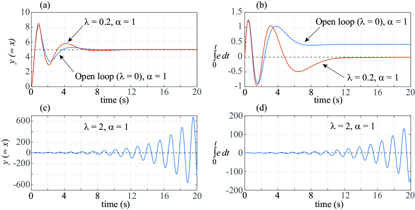
Figure 4: Step response and $e_{r}=\lim_{t\rightarrow\infty}\int_{0}^{t}e(\tau)d\tau$ for Eq. 35 under compensation of Fig. 2

The analysis above gives $c_{1}=0.3$, $c_{3}=0.21$, and $c_{4}\approx 21$, yielding $0<\lambda<0.0017$ as a sufficient condition for closed-loop stability. This is a conservative estimate of $\lambda$. However, from linearization of the closed-loop system around $x=r$, which is,

$$\dddot{x}+2\zeta\omega_{n}\ddot{x}+\omega_{n}^{2}\dot{x}+\omega_{n}^{2}\lambda(x-r)=0$$

the necessary and sufficient condition for local stability, using the Routh-Hurwitz criterion, is $0<\lambda<2\zeta\omega_{n}=1.4$. Simulation results are depicted in Fig. 4 for the open-loop case (i.e. $\lambda=0$) and for $\lambda=0.2,2$, with $\alpha=1(=1/\mbox{DC gain})$.

In Fig. 4(a), the step response of the closed-loop system, when $\lambda=0.2$, exponentially converges to step input $r=5$, as does the open-loop system ($\lambda=0$). In addition, Fig. 4(b) illustrates that $\int_{0}^{\infty}e(\tau)d\tau\neq 0$ for $\lambda=0$, and $\int_{0}^{\infty}e(\tau)d\tau=0$ for $\lambda=0.2$. However, when $\lambda=2$ the output and integral constraint values diverge, as shown in Fig. 4(c),(d), since the system is unstable for $\lambda=2>1.4$.

5 Conclusion

This paper demonstrates a method of shaping the transient step response of nonlinear systems using the compensation structure of Fig. 2, to satisfy a class of integral constraints. The method is applicable to SISO nonlinear systems that provide a stable step response and have a positive DC gain. Such nonlinear systems are plentiful, including hybrid energy systems where the aforementioned integral constraints are key to power management. First, the ability of the compensated system to satisfy the integral constraints while tracking step inputs is proven. Thereafter, analysis of first order nonlinear plants utilizing Converse Lyapunov Theorems establishes bounds on the integrator gain $\lambda$ where the closed-loop system is stable. The analysis assumes that the nonlinear plant has an exponentially or asymptotically stable response to step inputs, but does not require a detailed plant model. For higher order SISO nonlinear systems, the Normal Form is used to convert the original system to a chained-form of integrators and an internal dynamic. Here again, by assuming broad stability characteristics of the unknown plant, Converse Lyapunov Theorems are used to establish conditions for stability of the compensated system. Simulations demonstrate the efficacy of the study.

References

- [1] E. J. Davison, D. E. Davison, and R. Milman, “Transient response shaping, model based cheap control, saturation indices and mpc,” European journal of control, vol. 11, no. 4-5, pp. 288–300, 2005.
- [2] M. L. Liou, “A novel method of evaluating transient response,” Proceedings of the IEEE, vol. 54, no. 1, pp. 20–23, 1966.
- [3] M. R. Aaron and J. F. Kaiser, “On the calculation of transient response,” Proceedings of the IEEE, vol. 53, no. 9, pp. 1269–1269, 1965.
- [4] N. Mohsenizadeh, S. Darbha, and S. P. Bhattacharyya, “Synthesis of pid controllers with guaranteed non-overshooting transient response,” in 2011 50th IEEE Conference on Decision and Control and European Control Conference, pp. 447–452, 2011.
- [5] Y. C. Kim, L. H. Keel, and S. P. Bhattacharyya, “Transient response control via characteristic ratio assignment,” IEEE Transactions on Automatic Control, vol. 48, no. 12, pp. 2238–2244, 2003.
- [6] K. L. Moore and S. P. Bhattacharyya, “A technique for choosing zero locations for minimal overshoot,” IEEE Transactions on Automatic Control, vol. 35, no. 5, pp. 577–580, 1990.
- [7] K. Graichen, V. Hagenmeyer, and M. Zeitz, “A new approach to inversion-based feedforward control design for nonlinear systems,” Automatica, vol. 41, no. 12, pp. 2033 – 2041, 2005.
- [8] Y. Zhao and S. Jayasuriya, “Feedforward controllers and tracking accuracy in the presence of plant uncertainties,” Journal of Dynamic Systems, Measurement, and Control, vol. 117, no. 4, pp. 490–495, 1995.
- [9] G. M. Clayton, S. Tien, K. K. Leang, Q. Zhu, and S. Devasia, “A review of feedforward control approaches in nanopositioning for high-speed spm,” ASME Journal of Dynamic Systems, Measurement and Control, vol. 131, no. 6, p. 061101, 2009.
- [10] B. Haack and M. Tomizuka, “The Effect of Adding Zeroes to Feedforward Controllers,” Journal of Dynamic Systems, Measurement, and Control, vol. 113, pp. 6–10, 03 1991.
- [11] T. Yamaguchi and H. Hirai, “Control of transient response on a servosystem using mode-switching control, and its application to magnetic disk drives,” Control Engineering Practice, vol. 6, no. 9, pp. 1117 – 1123, 1998.
- [12] A. Hauksdóttir, “Analytic expressions of transfer function responses and choice of numerator coefficients (zeros),” IEEE transactions on automatic control, vol. 41, no. 10, pp. 1482–1488, 1996.
- [13] D. Newman, S.-W. Hong, and J. E. Vaughan, “The Design of Input Shapers Which Eliminate Nonzero Initial Conditions,” Journal of Dynamic Systems, Measurement, and Control, vol. 140, 05 2018. 101005.
- [14] C. Conker, H. Yavuz, and H. H. Bilgic, “A review of command shaping techniques for elimination of residual vibrations in flexible-joint manipulators,” Journal of Vibroengineering, vol. 18, no. 5, pp. 2947–2958, 2016.
- [15] C. P. Bechlioulis and G. A. Rovithakis, “Prescribed performance adaptive control for multi-input multi-output affine in the control nonlinear systems,” IEEE Transactions on Automatic Control, vol. 55, no. 5, pp. 1220–1226, 2010.
- [16] B. Fan, Q. Yang, S. Jagannathan, and Y. Sun, “Asymptotic tracking controller design for nonlinear systems with guaranteed performance,” IEEE Transactions on Cybernetics, vol. 48, no. 7, pp. 2001–2011, 2018.
- [17] D. Q. Mayne, “Control of constrained dynamic systems,” European Journal of Control, vol. 7, no. 2-3, pp. 87–99, 2001.
- [18] T. Das and S. Snyder, “Adaptive control of a solid oxide fuel cell ultra-capacitor hybrid system,” IEEE Transactions on Control Systems Technology, vol. 21, no. 2, pp. 372–383, 2012.
- [19] T. Allag and T. Das, “Robust control of solid oxide fuel cell ultracapacitor hybrid system,” IEEE Transactions on Control Systems Technology, vol. 20, no. 1, pp. 1–10, 2011.
- [20] B. Salih and T. Das, “Adaptive feedforward control of linear systems to satisfy integral constraints imposed on transients,” 2019 American Control Conference (ACC), pp. 5792–5797, 2019.
- [21] B. Salih and T. Das, “Transient Response of Linear Systems Under Integral Constraints,” Journal of Dynamic Systems, Measurement, and Control, vol. 142, 09 2020. 121007.
- [22] M. Morari, “Robust stability of systems with integral control,” IEEE Transactions on Automatic Control, vol. 30, no. 6, pp. 574–577, 1985.
- [23] H. K. Khalil, Nonlinear systems. Prentice hall Upper Saddle River, NJ, 3 ed., 2002.
- [24] D. E. Seborg and M. A. Henson, eds., Nonlinear Process Control. Prentice Hall, 1 ed., 1996.