Programmable quantum simulation of 2D antiferromagnets with hundreds of Rydberg atoms

Quantum simulation using synthetic systems is a promising route to solve outstanding quantum many-body problems in regimes where other approaches, including numerical ones, failGeorgescu et al. (2014). Many platforms are being developed towards this goal, in particular based on trapped ionsBlatt and Roos (2012); Monroe et al. (2020); Gärttner et al. (2017), superconducting circuitsSong et al. (2017); King et al. (2018); Kjaergaard et al. (2020), neutral atomsBloch et al. (2008, 2012); Gross and Bloch (2017); Browaeys and Lahaye (2020) or moleculesYan et al. (2013); Zhou et al. (2011). All of which face two key challenges: (i) scaling up the ensemble size, whilst retaining high quality control over the parameters and (ii) certifying the outputs for these large systems. Here, we use programmable arrays of individual atoms trapped in optical tweezers, with interactions controlled by laser-excitation to Rydberg statesBrowaeys and Lahaye (2020) to implement an iconic many-body problem, the antiferromagnetic 2D transverse field Ising model. We push this platform to an unprecedented regime with up to 196 atoms manipulated with high fidelity. We probe the antiferromagnetic order by dynamically tuning the parameters of the Hamiltonian. We illustrate the versatility of our platform by exploring various system sizes on two qualitatively different geometries, square and triangular arrays. We obtain good agreement with numerical calculations up to a computationally feasible size ($\mathbf{\sim 100}$ particles). This work demonstrates that our platform can be readily used to address open questions in many-body physics.

Figure 1: Emergence of antiferromagnetic ordering from the Rydberg blockade in square and triangular arrays. a, Illustration of the Rydberg blockade with two atoms, whereby the strong interactions prevent the simultaneous excitation of two atoms from the ground state (red circles) to the Rydberg state (blue circles) within the Rydberg blockade radius $R_{\rm{b}}$ at which $U=\hbar\Omega$. b,c Single-shot fluorescence images of ground state ($\left|\downarrow\right\rangle$) atoms in a ${14\times 14}$ square array and a 147-atom triangular array with an atomic separation of $a=10~{}\mu$m. b, Initial PM states and c, nearly perfect AF ordering.

Previous works demonstrated the potential of Rydberg-based quantum simulators with up to a few tens of atomsBernien et al. (2017); Keesling et al. (2019); Lienhard et al. (2018), including high-fidelity manipulations Levine et al. (2019); Omran et al. (2019); Madjarov et al. (2020). In particular, the transverse field Ising model (TFI) has been studied in 1D with up to 51 atomsSchauß et al. (2015); Bernien et al. (2017); Keesling et al. (2019), in 2D square arrays, but with a limited degree of coherenceLienhard et al. (2018); Guardado-Sanchez et al. (2018) making it difficult to observe genuine quantum features, and recently in 3D with 22 atomsSong et al. (2020). Here we implement the TFI in 2D, combining much larger atom numbers (up to $\sim 200$) and a high degree of coherence. In our implementation, we explore two geometries which exhibit qualitatively different phase diagrams: the bipartite square lattice and the geometrically frustrated triangular latticeWannier (1950). On the square lattice, we prepare the Néel state characteristic of antiferromagnets with unprecedented probability. On the triangular lattice, we observe for the first time, the creation of two distinct antiferromagnetic orders. The large number of atoms involved makes direct comparison between experimental results and the best numerical simulations extremely challenging. To validate the dynamics of our simulator we have pushed matrix product state simulations to their limit and are able to simulate the dynamics of up to 100 atoms in 2D. We obtain an impressive agreement between the simulation and the experiment up to this number, which is one of the largest for which a direct comparison has been performed. Finally, by comparing the experiment to classical Monte Carlo calculations we demonstrate that our results cannot be reproduced by a classical equilibrium distribution at the same mean energy, and that the experiment features an enhanced probability of finding classical ground states.

For arrays of atoms coupled by the (repulsive) van der Waals interaction, when excited to Rydberg states, the Hamiltonian of the TFI model is:

$$H_{\rm{Ryd}}=\sum_{i<j}U_{ij}n_{i}n_{j}+\frac{\hbar\Omega}{2}\sum_{i}\sigma^{x}_{i}-\hbar\delta\sum_{i}n_{i},$$ (1)

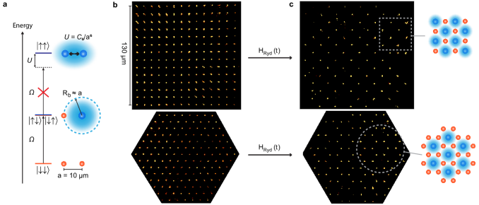
where the Rydberg and ground states are mapped onto the (pseudo-) spin states $\left|\uparrow\right\rangle$ and $\left|\downarrow\right\rangle$, respectively. Here ${U_{ij}=C_{6}/{r_{ij}^{6}}}$ is the van der Waals interaction, $r_{ij}$ is the distance between atoms $i$ and $j$, $n_{i}=\left|\uparrow\right\rangle\left\langle\uparrow\right|_{i}=(1+\sigma_{i}^{z})/2$, and $\sigma_{i}$ are the usual Pauli matrices. The two spin states are coupled via a laser field with a Rabi frequency $\Omega$ and a detuning $\delta$, which act as transverse and longitudinal fields, respectively. Antiferromagnetic (AF) ordering in the system appears as a consequence of the strong interactions characterised by the Rydberg blockade radius $R_{\rm{b}}$, as illustrated in Fig. 1aJaksch et al. (2000). The type of antiferromagnetic ordering depends on the geometry of the array and the Hamiltonian parameters.

Figure 2: The Ising model on a square lattice. a, Sketched bulk phase diagram for the square lattice. The inset shows the sweep shape with $t_{\rm off}$ the switch-off time of the excitation laser. The corresponding trajectory in the phase diagram is shown as a red arrow. b, State histogram for the ${8\times 8}$ array at the end of the sweep. The insets show fluorescence images of the two perfect AF states, which are obtained with 2.5% probability. c, Growth of the staggered magnetisation during the sweep for the $6\times 6$ and $10\times 10$ arrays. The blue circles are experimental results with standard errors on the mean smaller than the markers size. The error bar on the final point is indicative of the long-term stability of the machine (see Sec. .3.4). MPS simulations without (dashed line) and with (grey lines) experimental imperfections for which 50 ($6\times 6$), 77 ($10\times 10$) disorder instances are shown, with their average shown in black. The vertical dotted lines correspond to the turning points in the sweep. d, Final staggered magnetisation histograms for the ${10\times 10}$ and ${14\times 14}$ arrays and e, corresponding correlation maps, with MPS results shown in the lower half for the ${10\times 10}$ array.

We create defect-free square and triangular arrays of respectively up to 196 and 147 ⁸⁷Rb atoms using an optimised atom-by-atom assembly protocolSchymik et al. (2020) (see Fig. 1b). We define $\left|\downarrow\right\rangle=\left|5S_{1/2},F=2,m_{\rm{F}}=2\right\rangle$ and $\left|\uparrow\right\rangle=\left|75S_{1/2},m_{\rm{J}}=1/2\right\rangle$, which are coupled via the intermediate state $\left|6P_{3/2},F=3,m_{\rm{F}}=3\right\rangle$ with two counter-propagating laser beams of wavelength 420 nm and 1013 nmLevine et al. (2018) (see Sec. .1). We achieve a single atom excitation probability of $99\%$ and a coherence time $\sim 20$ times longer than in our previous workLienhard et al. (2018) (see Sec. .3.1). We use arrays with atomic spacing $a=10~{}\mu$m, leading to a nearest-neighbour interaction of $U/h\simeq 1.95{\;\rm MHz}$.

To probe the phase diagram of $H_{\rm{Ryd}}$ we sweep $\Omega(t)$ and $\delta(t)$, and transfer the system from its initial paramagnetic (PM) ground state $\left|\downarrow\downarrow\dots\downarrow\right\rangle$ into the AF phase. A quantum phase transition (QPT) separates these two phases. Ideally, one would adiabatically drive the system such that it remains in the instantaneous ground state. However, the energy gap at the QPT decreases with the atom number $N$, ($\sim 1/\sqrt{N}$ on a square lattice and $\sim\exp(-\alpha N)$ for the triangular latticeJanke and Villanova (1997); Laumann et al. (2012)). This leads to time scales which are experimentally impractical due to decoherence effects. Hence, we choose sweep times ($\sim 6~{}\mu$s) which are short enough to avoid sizeable decoherence but sufficiently long to quasi-adiabatically probe the phase diagram (see Sec. .3.2). We record fluorescence images of the atoms remaining in $\left|\downarrow\right\rangle$. Single-shot images, showing prepared, nearly perfect AF ordering on the square and triangular arrays, are shown in Fig. 1c. For the results presented here, we typically repeat the sequence 1000 times.

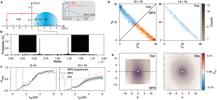
We first focus on the square lattice,using arrays of size ${N=L\times L}$, with even $L$ so that the two Néel states have the same energy. In Fig. 2a we sketch the (bulk) phase diagram. In the case of the van der Waals interaction implemented here, the AF phase region is expected to extend up to $\hbar\Omega_{\rm c}\approx 1.25\ U$ at $\hbar\delta\approx 4.66\ U/2$ (Ref. 29). More complex phasesSamajdar et al. (2020) appear at the lower and upper boundaries of $\hbar\delta/U$ in the AF region. The applied sweeps are shown in Fig. 2a, with the QPT being crossed during the ramp down of $\Omega(t)$. Figure 2b presents an experimental histogram of the states recorded at the end of the sweep for the ${8\times 8}$ array. Remarkably, out of $2^{64}\simeq 2\times 10^{19}$ possible states, we obtain a perfectly ordered state with a probability of $\sim$2.5%, as can be seen by the two prominent peaks. The fluorescence images show the two corresponding Néel states. To characterise the magnetic ordering of the states prepared during the sweep, we measure the order parameter, which is the normalised staggered magnetisation ${m_{\rm{stag}}=\langle|n_{\rm{A}}-n_{\rm{B}}|\rangle/(N/2)}$, giving the difference in the number of excitations on each sublattice $(\rm{A,B})$, averaged over many realisations. The two perfect AF states correspond to one of the two sublattices being fully excited, such that $m_{\rm{stag}}=1$. We access the dynamics of the system during the sweep by rapidly turning off the excitation laser at different times $t_{\rm{off}}$ (see Fig. 2a). Fig. 2c presents the evolution of $m_{\rm{stag}}$ for the ${6\times 6}$ and ${10\times 10}$ arrays, using the same sweep. Over the first $1.5~{}\mu$s of the sweep the system is in the PM phase, where fluctuations lead to small but finite $m_{\rm stag}\sim 1/\sqrt{N}$. We then observe the growth of $m_{\rm stag}$ during the drive of the system from the PM to the AF phase.

To benchmark our platform, we perform a systematic comparison of the dynamics with matrix product state (MPS) numerical simulations (see Sec. .2). We consider both the programmed and the real parameters, the latter of which include independently calibrated experimental imperfections, with the exception of decoherence effects (see Sec. .3.3). For the ${6\times 6}$ array, we observe a good agreement between the experimental results and the MPS simulations, for both situations. For the ${10\times 10}$ array, the experiment and the real MPS simulations also agree well. The difference between the programmed and the real MPS simulations highlights that the imperfections have a more severe impact on larger systems. Additionally, the reduced final value of $m_{\rm stag}$ for the programmed MPS on the $10\times 10$ array indicates that as the system size grows, adiabaticity is indeed harder to achieve.

We now characterise the final state obtained at the end of the sweep ($\Omega=0$). Firstly, we visualise the shot-wise contributions to $m_{\rm{stag}}$ using a 2D histogram of the probability $P(n_{\rm{A}},n_{\rm{B}})$ of the $\left|\uparrow\right\rangle$ populations $n_{\rm{A}}$ and $n_{\rm{B}}$ of the two sublattices A, B. Here, the two Néel states appear as points at ($N/2,0$) and ($0,N/2$). The results are plotted in Fig. 2d for the ${10\times 10}$ and ${14\times 14}$ arrays. For both systems we observe the presence of points along the diagonal highlighting that the average Rydberg density is $\sim 50\%$. For the ${10\times 10}$ we observe a conglomeration of points around the two corners belonging to the Néel states. Because of the imperfections and the scaling of the energy gap, the state preparation becomes more challenging with increasing system size. The elongated histogram for the $14\times 14$ array demonstrates that, remarkably, we prepare strongly AF ordered states ($m_{\rm stag}\sim 0.4$), even for such large systems. This is also evident in the fluorescence image in Fig. 1c, containing 184 atoms (out of 196) obeying AF ordering. For a comparison with simulations, we have devised an algorithm to stochastically sample the MPS wavefunction, thereby obtaining snapshots as in the experiment (see Sec. .2.2). The lower half of Fig. 2d shows the so-obtained histogram for the $10\times 10$ lattice, which matches the experiment very well. For even larger atom numbers, accurate MPS simulations become intractable.

Secondly, we compute the connected spin-spin correlation function defined as

$$C_{k,l}=\frac{1}{N_{k,l}}\sum_{i,j}{\langle n_{i}n_{j}\rangle-\langle n_{i}\rangle\langle n_{j}\rangle},$$ (2)

where the sum runs over all pairs of atoms $i,j$ separated by $k\textbf{e}_{1}+l\textbf{e}_{2}$, with $\textbf{e}_{1(2)}$ denoting the two vectors of the underlying lattice, and $N_{k,l}$ being the number of such pairs. Figure 2e shows the $C_{k,l}$ correlation maps corresponding to the $m_{\rm{stag}}$ histograms shown in Fig. 2d. The plots display the alternation of correlation and anti-correlation, expected for AF ordering, whose values would be $\pm 1/4$ for the Néel state. The spatial decay of the correlations is well described by correlation lengths of $\xi\simeq 7a$ and $5.5a$ for the two system sizes respectively, showing that the sweeps produce highly AF ordered states. Again we observe very good agreement between experimental and real MPS results for the ${10\times 10}$ array, confirming that the simulations capture well the experimental conditions (for a real-time analysis of the correlations during the sweep, see Sec. .3.5).

To further quantify the AF ordering, we analyse the distribution of antiferromagnetic cluster sizes Stoli and Domb (1979). For each run of the experiment, we decompose the snapshot into individual clusters obeying local AF ordering (see examples in Fig. 3a,b). We count the number of atoms inside each individual cluster, and record the largest size, $s_{\rm max}$. From the full set of snapshots we reconstruct the probability distribution $P(s_{\rm max})$. For a perfectly AF-ordered state, this distribution presents as a single peak of unit probability at ${s_{\text{max}}=N}$, while imperfect ordering shows up as a distribution broadened towards smaller $s_{\rm max}$. In Fig. 3c,d we show $P(s_{\rm max})$ at two instants during the sweep for the ${10\times 10}$ array (blue bars). Even at intermediate times, shortly after entering the AF region (Fig. 3c), we observe the presence of significant AF ordering, as the distribution is centred around large values of $s_{\text{max}}$. At the end of the sweep (Fig. 3d), Néel states are observed, as shown in Fig. 3b, and more than 27% of the shots feature AF states with clusters missing at most 10 sites.

Figure 3: Quantum real-time evolution versus classical equilibrium: a, b, Fluorescence images on a ${10\times 10}$ array illustrating how we extract the largest AF domains comprising of $s_{\rm max}$ sites, indicated by the blue boundaries. c, d, Distributions of $s_{\rm max}$ during c and at the end of d the sweep (blue), compared to the classical equilibrium result (yellow) with the corresponding hypothetical temperature $T_{\rm hyp}$.

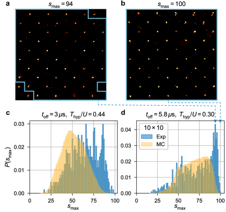
The fact that we obtain a distribution of final states raises the question whether the system has thermalised during the finite duration of the sweep Bernien et al. (2017); Kim et al. (2018). To answer this question, we compare the observed distribution $P(s_{\rm max})$ to the corresponding distribution obtained from a classical equilibrium setup with a hypothetical temperature $T_{\rm hyp}$. We focus on a classical description for two reasons: i) the classical energy is the one accessible in the experiment and ii) at the end of the sweep, $\Omega=0$ and the quantum and classical statistical mechanics descriptions coincide.

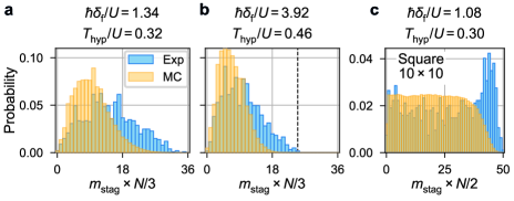
To determine $T_{\rm hyp}$ we match the classical Ising energy $E_{\rm class}(t_{\rm off})$ of the experimental system with $E^{\rm MC}_{\rm class}(T)$ from the corresponding classical statistical mechanics system for a given temperature $T$ estimated from a Monte Carlo (MC) sampling . We refer to Sec. .4.1 for a thorough discussion of $T_{\rm hyp}$ during the sweep. In Fig. 3c,d, we show $P(s_{\rm max})$ for the corresponding classical equilibrium distributions (orange bars), and observe that they are centered at a significantly smaller $s_{\text{max}}$, and do not reproduce the distribution of the experimental results. In particular, the probability of finding perfectly ordered states is much higher in the experiment. An equivalent analysis of the MPS real-time evolution shows similar features (see Sec. .4.3). Our analysis therefore reveals that despite residual imperfections, the experiment does not thermalise during the state preparation protocol and can only be consistently reproduced by a unitary quantum mechanical real-time description. Furthermore, the enhanced probability of finding the targeted classical states is promising for future applications of the Rydberg platform, e.g., as a quantum annealer to solve optimisation problems of various typesPichler et al. (2018); Henriet (2020); Serret et al. (2020).

Figure 4: Antiferromagnetic ordering on a triangular array. a, Sketched bulk phase diagram for the triangular lattice. The red arrows show the sweeps used to prepare the phases at filling $1/3$ and $2/3$. b, Growth of the staggered magnetisation during the sweep for a 75-atom array. The blue circles are experimental results with standard errors on the mean smaller than the markers size. The error bar on the final point is indicative of the long-term stability of the machine (see Sec. .3.4). MPS simulations without (dashed line) and with (grey lines) experimental imperfections for which 50 disorder instances are shown, with their average shown in black. The vertical dotted lines correspond to the turning points in the sweep. c, Final experimental correlation maps and d, corresponding staggered magnetisation histograms plotted in the complex plane for the 75, 108 and 147 site triangular arrays for the sweep preparing the $1/3$ phase. For the 75 and 108 site arrays the lower half of the histograms show the analogous MPS results. e, Final experimental correlation map and g, corresponding staggered magnetisation histogram for the 108 site triangular array for the sweep preparing the $2/3$ phase. The lower half in f shows corresponding MPS results.

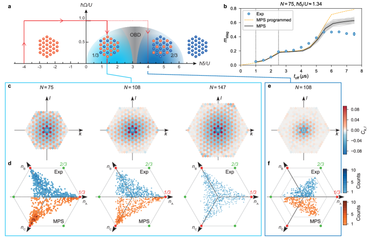
Having explored the square lattice we now consider the more complex triangular array. Here, the TFI model features a richer phase diagram, with prominent ordered phases at $1/3$ and $2/3$ Rydberg filling, as sketched in Fig. 4a. The $1/3$ phase is the analogue of the AF ordering on the square lattice, where the Rydberg blockade prevents neighbouring sites from being excited simultaneously, leading to one of the three sublattices being filled with Rydberg excitations, illustrated in Fig. 1c. The $2/3$ phase is the “particle-hole” inverse of this, with two sublattices being fully excited and one sublattice containing ground state atoms. In between these phase regions, at 1/2 filling, the classical Ising model ($\Omega=0$) is strongly frustrated for nearest-neighbour interactions, with an exponentially large (in $N$) ground state manifold Wannier (1950). Finite $\Omega$ stabilises yet another ordered phase in a process called “order by disorder” (OBD) Villain et al. (1980); Moessner et al. (2000); Moessner and Sondhi (2001); Isakov and Moessner (2003); Fey et al. (2019); Koziol et al. (2019).

To explore the triangular phase diagram, we consider hexagonal clusters of various sizes, built shell by shell around a central three-atom triangle (see Fig. 1b). We apply the sweeps shown in Fig. 4a for two different final detunings $\delta_{\text{f}}$, to create the $1/3$ and the $2/3$ phases. To quantify the state preparation process, we again measure the temporal dynamics of the order parameter, the normalised staggered magnetisation. For the triangular array, this is defined as $m_{\text{stag}}=\langle\left|n_{\rm{A}}+{\rm e}^{i2\pi/3}n_{\rm{B}}+{\rm e}^{-i2\pi/3}n_{\rm{C}}\right|\rangle/(N/3)$, where $n_{\rm A,B,C}$ is the Rydberg population on each of the three sublattices. We plot the results in Fig. 4b for the experiment and two types of MPS simulations (programmed and real) for a 75-atom array, with $\delta_{\text{f}}$ chosen to prepare the $1/3$ phase. We observe the growth of the AF ordering both in the experiment and the simulations, which agree very well during the first 5 $\mu$s of the sweep. After this the experimental results plateau at a lower value of $m_{\mathrm{stag}}$ than expected from the MPS. The inclusion of experimental imperfections decreases the final value of $m_{\rm stag}$, however, there is still a discrepancy with the experimental results. A possible explanation could be the enhanced sensitivity of the QPT from paramagnetic to the $1/3$ AF phase (believed to be first-orderJanke and Villanova (1997)) to the residual experimental imperfections not included in the MPS simulation. Confirming the origin of this effect will be the subject of future work.

To further characterise the prepared final states we consider $C_{k,l}$, defined similarly to Eq. (2). Here, the perfect AF state would have $C_{k,l}=+2/9$ and $-1/9$ for correlated and anti-correlated sites, respectively. In Fig. 4c,e we show the final state correlation maps for the 1/3 (2/3) phases on atom arrays of 75, 108 and 147 sites (108 sites). We observe a pattern characteristic of three-sublattice ordered states, throughout almost the entire bulk of our systems, with a correlation length $\xi\sim 3$—$3.7a$ for the $1/3$ phase and $\xi\sim 2a$ for the $2/3$ phase. In Fig. 4d,f we plot the corresponding distributions of the complex order parameter. For perfectly ordered $1/3$ ($2/3$) systems, one would expect peaks at the three corners of the bounding hexagon, marked by red (green) dots. We observe correspondingly aligned triangular distributions with good agreement between the experimental and MPS results. There is a higher accumulation of points at the corners in the MPS results, which corresponds to a higher value of $m_{\mathrm{stag}}$. While the distributions spread almost fully to the corners in the $1/3$ phase results, for the $2/3$ phase the size of the triangle is visibly reduced. This reduction is due to finite-size cluster effects: the boundary is filled with Rydberg excitations which reduces the maximal possible extent of the distribution to the inner hexagon (dashed lines) (see Sec. .5.1). To our knowledge, the above results are the first observations of the 1/3 and 2/3 phases using a quantum many-body system. Despite the experimental imperfections, and the finite sweep duration, we are able to produce highly-ordered states on even the largest 147-atom array. This is highlighted in Fig. 1c showing a fluorescence image of the 1/3 phase on the 147-atom array with almost perfect AF ordering. Finally, similar to the square array, we observe an enhanced probability of finding highly ordered states compared to a classical equilibrium system at the same energy, as revealed by experimental order parameter distributions which are centred at larger values (see details in Sec. .5.2).

As a conclusion, we have probed the quantum dynamics of Ising magnets in square and triangular geometries, beyond situations which can be exactly simulated classically. We have validated the experimental results with comprehensive numerical simulations up to computationally feasible sizes. We have shown a high degree of coherence and control, over a large number of atoms. Combined, this demonstrates that our platform is now able to study quantum spin models in regimes beyond those accessible via numerical investigations. We have also identified a potential advantage of Rydberg quantum simulators to prepare targeted classical states, compared to classical equilibrium systems. Natural extensions of this work include a thorough investigation of the dynamics of the 2D quantum phase transition, and further explorations of the effects of frustration, in particular the observation of the elusive OBD phase. Finally, our benchmark provides a roadmap for improving the platform even further thus opening exciting prospects beyond quantum simulation, e.g. for optimisationPichler et al. (2018); Serret et al. (2020), quantum sensingMadjarov et al. (2019); Norcia et al. (2019) and quantum computingSaffman et al. (2010); Henriet et al. (2020); Morgado and Whitlock (2020).

Author contributions

^∗PS, MS, HJW, and AAE contributed equally to this work. PS, HJW, DB, KS, and VL carried out the experiments. MS, AAE, L-PH and TCL performed the simulations. All authors contributed to the data analysis, progression of the project, and on both the experimental and theoretical side. All authors contributed to the writing of the manuscript. Correspondence and requests for materials should be addressed to Pascal Scholl.

Ethics Declaration

The authors declare no competing interests.

Supplementary Information

.1 Experimental set-up

Our experimental setup, described in detail in Ref. 48, is based on arrays of single atoms trapped in optical tweezers. In order to create defect-free arrays consisting of $N$ atoms, we begin with a stochastically loaded array containing $>2N$ traps and then, using a single, moving optical tweezer trap, rearrange the atoms into the desired configuration. Optimisation of the rearrangement algorithms and the introduction of multiple cycles Schymik et al. (2020) have enabled us to create arbitrary arrays with up to 200 atoms.

Following the rearrangement, the atoms are optically pumped into the ground state $\left|\downarrow\right\rangle=\left|5S_{1/2},F=2,m_{F}=2\right\rangle$ in the presence of a static magnetic field of 7 G with $99.9\%$ efficiency. The tweezers are then switched off for the duration of the sweeps. We use the Rydberg state $\left|\uparrow\right\rangle=\left|75S_{1/2},m_{J}=1/2\right\rangle$ with a lifetime $\tau=175\;\mu{\rm s}$, and van der Waals coefficient $C_{6}/h=1947\;{\rm GHz}\cdot\mu{\rm m}^{6}$. To excite the atoms from $\left|\downarrow\right\rangle$ to $\left|\uparrow\right\rangle$, we drive a two-photon transition using counter-propagating laser beams with wavelengths 420 nm and 1013 nm, via the intermediate state $\left|6P_{3/2},F=3,m_{\rm{F}}=3\right\rangle$ with a lifetime of 113 ns. We use two Ti:Sapphire lasers (M-Squared), because of their intrinsic low phase noise at high frequencyde Léséleuc et al. (2018). One, operating at 840 nm, is frequency doubled to 420 nm with up to 2 W, and the second, at 1013 nm, seeds an AzurLight Systems fibre amplifier delivering up to 10 W. The 420 nm light is fibre coupled to the experiment, whilst the 1013 nm light is free-space. The $1/e^{2}$ radii and maximum powers of the lasers at the position of the atoms are $w_{420}=250~{}\mu$m, $P_{420}=350$ mW, and $w_{1013}=130~{}\mu$m, $P_{1013}=5$ W, allowing for Rabi frequencies of up to $\Omega_{420}=2\pi\times 200$ MHz and $\Omega_{1013}=2\pi\times 50$ MHz. To limit the spontaneous emission, the lasers are detuned by $2\pi\times 700$ MHz from the intermediate state, resulting in a maximum effective Rabi frequency of $\Omega=2\pi\times 7$ MHz.

To detect the state of the atoms the tweezers are turned back on, recapturing atoms in $\left|\downarrow\right\rangle$, which we then image. The atoms in $\left|\uparrow\right\rangle$ are repelled from the tweezers and hence are not imaged. This detection method features imperfections, described in detail in Ref. 49, which result in two types of errors. Firstly a false positive, with probability $\varepsilon$, where a ground-state atom is lost and misidentified as a Rydberg atom, and secondly a false negative, with probability $\varepsilon^{\prime}$, where a Rydberg atom decays quickly, is recaptured and hence, misidentified as a ground-state atom. The results presented in the main text have $\varepsilon=1\%$ and $\varepsilon^{\prime}=3\%$.

.2 Matrix Product States

In order to verify the experimental results we compare to numerical simulations. For the large atom numbers used in this work Exact Diagonalisation methods are too expensive and so we employ matrix product state (MPS) methods as described in this section.

.2.1 Method

Matrix product state methods are well documented in the literature Schollwöck (2011); Paeckel et al. (2019), so we focus here on the aspects important for the discussion in this paper.

MPS methods approximate the physical state by a linear network of $N$ tensors, one at each site. Initially developed for one-dimensional many body systems, the method is also successful on two-dimensional systems of limited width Stoudenmire and White (2012). In our case the ${L\times L}$ square lattice is mapped row-by-row to a linear tensor network, for the triangular arrays the mapping is similar except that the rows have variable width. The MPS approximation is controlled by the bond dimension $\chi$, which limits the maximum amount of entanglement between consecutive subsystems. An MPS with bond dimension $\chi$ can exhibit at most an entanglement entropy of $S=\ln(\chi)$ for a bipartition into two connected chains.

For ground state wavefunctions of gapped, local Hamiltonians one expects the entanglement entropy of subsystems to follow an area law Eisert et al. (2010). This means that the entanglement entropy between two subsystems is proportional to the length (or area) of the perimeter of the subsystems, and not proportional to their volume. When considering a time-dependent situation as we do here, the entanglement structure can become more complicated, and, for example, change to a volume law if long times after a quench are studied. Since we typically fix the duration of our sweeps while scaling up the system size, we are effectively still dealing with an area-law situation. Applying these considerations to the square and the triangular lattice arrays, we are simulating systems with a maximal entanglement entropy between subsystems proportional to the width of the clusters, i.e. $S\sim L$ for the square arrays. This translates into a scaling of the required bond dimension $\chi\sim\exp[\alpha L]$ for simulations of constant accuracy. Based on this scaling we are able to reach widths of $L=10$ for the square lattice and a similar width for the triangular array ($N=108$) with a bond dimension of up to $\chi=512$, see discussion below.

For the unitary time evolution we use the time-dependent variation principle (TDVP) Haegeman et al. (2011, 2016) which works by projecting the Hamiltonian onto the state’s tangent space and then applying the time evolution operator for a small time-step. At each step we can either use a single-site or a two-site algorithm, the latter of which allows for growth of the MPS’ bond dimension. The simulation starts in the initial product state which evolves in time according to the Hamiltonian Eq. (1), at first using the two-site variant until the bond dimension is saturated to a certain chosen value $\chi$, and then we switch to the single-site variant for a significant performance increase.

For every system size these simulations are repeated for 30 to 70 different realisations of random lattice positions, and include other experimental uncertainties, described in Sec. .3.3. We use the implementation of TDVP provided by the python package TeNPy Hauschild and Pollmann (2018). The computationally most expensive simulations for the $10\times 10$ square with a bond dimension of $\chi=512$ take up to 14 days for a single disorder instance. We use computer clusters to simultaneously simulate around 50 disorder instances.

.2.2 Sampling

The experiment delivers snapshots of the state of the system projected to the Rydberg Fock space. From this data, one can determine local densities, density correlation functions, and sublattice histograms. These quantities can also be obtained from Exact Diagonalization, as well as the classical and quantum Monte Carlo algorithms. With the MPS method local densities and correlations can also be obtained easily by tensor contractions. However, the sampling of the Fock space snapshots is not so simple. While the weight of a given configuration can be efficiently obtained by contracting the MPS network with the snapshot configuration as the input on the physical legs, it is less straightforward to find the most probable configurations out of the $2^{N}$ possible states.

We devised an algorithm to generate statistically independent snapshots of a given MPS wave function:

1. Pick an arbitrary site $i$ among the $n$ unprojected sites of the normalised MPS, and determine the diagonal elements of the single site reduced density matrix $p_{g}^{(i)}$ and $p_{e}^{(i)}$ (for the ground state ($\left|\downarrow\right\rangle$) and excited state ($\left|\uparrow\right\rangle$) respectively) which sum up to one.

2. Draw a random number $r\in[0,1]$ and select $g$ if $r<p_{g}^{(i)}$ or else select $e$. Apply the single site projector for the selected subspace, effectively fixing the physical leg of that site’s tensor.

3. The remaining MPS with $n-1$ unprojected sites is normalised to the value of $p_{g|e}^{(i)}$, depending on the randomly selected subspace in the previous step. Thus we divide the MPS by that value to normalise it to 1.

4. Repeat the process until there are no unprojected sites remaining.

It does not matter whether the sites to be projected are picked randomly or in sequence, however the latter provides the opportunity to optimise the generation of thousands of snapshots by pre-contracting the tensor network. We usually generate 1000 to 10000 snapshots for each data point shown. The algorithm presented here is related to the “collapse” step in “Minimally entangled typical thermal state” MPS algorithms for finite temperature simulationsStoudenmire and White (2010).

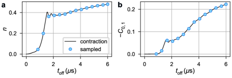
In Fig. 5 we compare the average Rydberg density $n=\sum_{i}\langle n_{i}\rangle/N$ and the correlator $C_{0,1}$ during the time-evolution on a ${10\times 10}$ square lattice computed by standard tensor contractions (black curves) to their value from a sample average of 1000 snapshots, generated with the algorithm discussed above (blue dots). The perfect agreement demonstrates that the devised algorithm successfully samples the MPS wave function.

Figure 5: MPS Sampling. a, Average Rydberg density and b nearest-neighbour correlation function during the MPS state dynamics on the ${10\times 10}$ square lattice. The black lines show the observables computed from standard tensor contraction, the blue dots show the corresponding sample average of 1000 generated snapshots.

.2.3 Bond dimension $\chi$ dependence

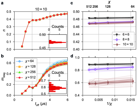
Due to the aforementioned scaling of the computational complexity of the problem with $\chi$, a trade-off between accuracy and available computational resources has to be achieved. In Fig. 6 we analyse the scaling of relevant observables used in this paper with the bond dimension $\chi$, including experimental imperfections. Both the average Rydberg density $n$ (Fig. 6a) and the order parameter $m_{\rm stag}$ (Fig. 6b) show only a very weak dependence on $\chi$ for small times $t_{\rm off}$. As expected, for larger times, the variation with $\chi$ becomes stronger, in particular for $m_{\rm stag}$. Nevertheless, this variation remains small even at the end of the sweep and, notably, the uncertainty from different interaction disorder instances, shown by the shaded regions, is comparable to the variation between the lowest and largest bond dimensions.

In Fig. 6c,d, we plot $n$ and $m_{\rm stag}$ at the end of the sweep versus $1/\chi$ for different system sizes. For $L=6$, simulations with up to $\chi=512$ reveal a nice convergence for these observables, and the larger systems show only a slight dependence on $\chi$. The variation resulting from $\chi$ is again smaller than that of the random $U_{ij}$, illustrated by the lighter lines.

To summarise, our MPS simulations for systems up to $L=10$ are reliable to characterise and benchmark the experimental results, although they might not be fully converged in $\chi$ with regard to other observables, such as the entanglement entropy. Finally, we want to mention that reliable simulations of the dynamics for the largest experimental results achieved in this paper ($L=14$) seem to be out of reach with currently available computational hardware, because of the exponential scaling of $\chi$ with linear system size $L$.

Figure 6: Scaling of observables with MPS bond dimension $\chi$. a, Rydberg density and b, order parameter during the MPS state dynamics, including experimental imperfections, for different $\chi$ on the $10\times 10$ square lattice. The insets show the distribution due to the multiple $U_{ij}$ disorder realisations, at final $t_{\rm off}=6\ \mu{\rm s}$ for $\chi=256$. Scaling of c, $n$ and d, $m_{\rm{stag}}$ with $\chi$ at the end of the state preparation protocol for different system sizes. The lightly coloured lines show the multiple disorder instances.

.3 Benchmarking the platform

In this section we discuss experimental imperfections, and systematically compare the results of the experiment with numerical simulations. We first investigate the coherence of the laser excitation for a single atom, and then introduce the imperfections relevant to the many-atom case.

.3.1 Coherence of single-atom laser excitation

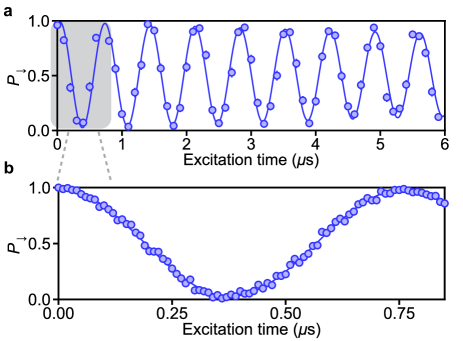
To investigate the efficiency and the coherence of the Rydberg excitation on a single atom, we drive Rabi oscillations between the $\left|\downarrow\right\rangle$ and $\left|\uparrow\right\rangle$ states. The results are shown in Fig. 7a, where the oscillations are fitted by a damped sine $Ae^{-\Gamma t}\cos(\Omega t)+B$. We obtain a decay rate $\Gamma=0.04(1)\mu\text{s}^{-1}$ due to spontaneous emission from the intermediate state and to the shot-to-shot fluctuations of the laser power ($\sim 1\%$). In Fig. 7b, we show a magnification of the first period, from which we measure a 97.3% probability of transferring a single atom to the $\left|\uparrow\right\rangle$ state with a $\pi$-pulse. For this experiment, following the methods outlined in Ref. 49, we measure $\varepsilon=0.4\%$ and infer from simulation using the experimental parameters $\varepsilon^{{}^{\prime}}=1.9\%$. When accounting for these detection errors, we extract a probability of 99.1% to transfer a single atom to the $\left|\uparrow\right\rangle$ state.

Figure 7: Testing the coherence of the Rydberg-excitation on a single atom. a, Rabi oscillations showing the probability of measuring the atom in $\left|\downarrow\right\rangle$ as a function of the excitation time. The line is a fit to the data by the function $Ae^{-\Gamma t}\cos(\Omega t)+B$, yielding $\Gamma=0.04(1)\mu\text{s}^{-1}$, $\Omega=2\pi\times 1.32(1)$ MHz, $A=0.975(6)$, and $B=0.507(3)$. b, High resolution measurement of the first period of the oscillation. Error bars are statistical and often smaller than marker size.

.3.2 Benchmarking the $4\times 4$ array

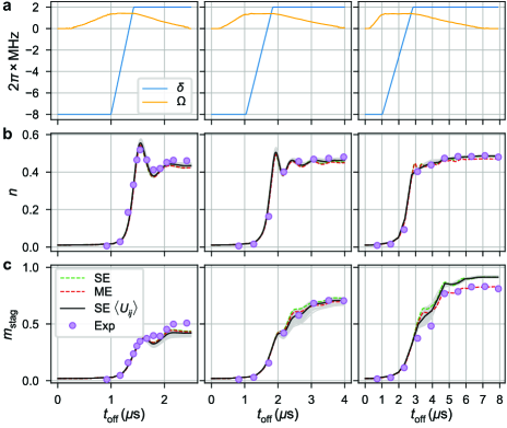
Here we investigate the dynamics of the system for different sweeps on the $4\times 4$ array. This system size can be fully simulated by solving the Schrödinger equation (SE), for which we include the detection errors (here $\varepsilon=1\%$ and $\varepsilon^{\prime}=3\%$). We assess the adiabaticity of the drive by performing three sweeps of durations $2.5~{}\mu\text{s}$, $4~{}\mu\text{s}$ and $8~{}\mu\text{s}$. The parameters of the sweeps, shown in Fig. 8a, are as follows: at a detuning $\delta/2\pi=-8$ MHz, $\Omega$ is linearly increased from 0 to $\sim 2\pi\times 1.4$ MHz, we then linearly sweep the detuning to $\sim 2$ MHz while keeping $\Omega$ constant, and finally decrease $\Omega$ to 0. As we drive a two-photon transition, the atoms experience a changing light shift as $\Omega$ is swept. We counteract this effect by changing $\delta$ accordingly. We use as observables the average Rydberg density $n$ and staggered magnetisation, $m_{\rm{stag}}$. For all sweeps we observe a good agreement between experiment and simulation, especially in the evolution of $n$. As expected, short sweeps lead to oscillations in the evolution of $n$ due to a failure to adiabatically drive the system. This is confirmed by the value of $m_{\rm{stag}}$ at the end of the sweep, $\sim 0.5$, which would be 1 if the sweep were adiabatic. As the sweep time increases, this oscillatory behaviour is reduced and the value of $m_{\rm{stag}}$ increases.

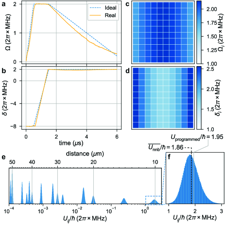
To understand the discrepancies between the SE results and the data we consider the potential experimental imperfections relevant for many-atom systems. The first is the disorder in atomic positions, which comes from two effects, (i) the static disorder in the trap positions (standard deviation $\sim 100$ nm), and (ii) the finite temperature (10 $\mu$K) of the atoms leading to shot-to-shot fluctuations in atom position with a standard deviation of $\sigma_{r}=170$ nm in the plane of the array, and $\sigma_{z}=1~{}\mu$m in the transverse direction. This results in a spatially correlated, non-gaussian distribution of the interaction energy $U_{ij}$ (see also Fig. 10e,f)Marcuzzi et al. (2017). This effect is included in simulations by repetitions with randomly assigned atom positions chosen from a Gaussian distribution with the mentioned standard deviations. We run simulations of the dynamics and average over many runs of the distribution in interaction energies. The runs are shown in Fig.8 in light grey, with the average SE$\langle U_{ij}\rangle$in black. This disorder has very little influence on the results and cannot explain the remaining disagreement. Another potential source of imperfection comes from the finite size of the 1013 nm beam, leading to inhomogeneous $\Omega$ and $\delta$ (due to the light-shift of the two-photon transition) across the array, however on this small system the inhomogeneity is found to have negligible effect on the results. The observation that the discrepancy is largest for the longest sweep duration indicates that decoherence plays an important role.

To study this effect we solve the Master equation (ME) for which the time evolution of the density matrix $\rho(t)$ is described by

$$\frac{d}{dt}\rho=-\frac{i}{\hbar}[H,\rho]+\mathcal{L}[\rho],$$ (3)

with a Liouvillian

$$\mathcal{L}[\rho]=\sum_{i}\frac{\gamma}{2}(2n_{i}\rho n_{i}-n_{i}\rho-\rho n_{i})$$ (4)

and a decoherence rate $\gamma=0.05~{}\mu$s^-1 which describes well the single-atom Rabi oscillation, when accounting for the shot-to-shot fluctuations of the laser power.

These results agree closely with the experimental data indicating that decoherence at the single particle level is sufficient to describe the system. We conclude from these studies that there is an optimised sweep duration which has to be (i) long enough to cross the gaps as adiabatically as possible and (ii) short enough to avoid strong decoherence effects. Throughout this paper, we limit the duration of the sweeps to be about $6-7.5~{}\mu\text{s}$ to fulfil these two conditions.

Figure 8: Benchmarking multiple sweeps on the $4\times 4$ array Time evolution of a, sweep shape, b, Rydberg density, and c, staggered magnetisation for three distinct sweeps (of durations $2.5~{}\mu$s, $4~{}\mu$s and $8~{}\mu$s) on the $4\times 4$ array. In (b, c) experimental data is shown in purple circles, the green (red) dashed line shows solutions to the Schrödinger (Lindblad master) equation. Solid grey lines show solutions of the Schrödinger equation for several random instances of the interaction disorder (see text), the black line is the average over these instances.

.3.3 Effect of imperfections on larger arrays

For larger arrays we use the matrix product state (MPS) method, described in detail in Sec. .2 to calculate the dynamics of the systems during the sweeps.

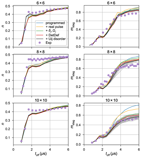
We first perform the programmed simulation, without experimental imperfections, for the $6\times 6$, $8\times 8$, and $10\times 10$ arrays, using the same sweep for each array. Figure 9 shows the evolution of $n$ and $m_{\rm{stag}}$, with the experimental data as purple points, and the blue line showing the MPS results. We find good agreement over the first $1.5$ $\mu$s after which we observe an overshoot in the experimental results in both $n$ and $m_{\rm stag}$ for all system sizes. We also observe that $m_{\rm stag}$ eventually saturates on the experiment at lower values than the MPS, and that this effect worsens for larger systems.

We therefore include in the MPS the imperfections discussed in the previous section, and illustrated in Fig. 10 for the $10\times 10$ array, starting from the experimentally measured sweep shape, adding the inhomogeneous fields $\delta_{i}$, $\Omega_{i}$, the detection deficiency and, finally, the shot-to-shot fluctuations of the interaction energies caused by the fluctuating atom positions. The results are shown in Fig. 9. The imperfections have very little effect on $n$, and are not able to explain the overshoot, in $n$ and $m_{\rm stag}$, at intermediate times. However, at later times we observe better agreement for all system sizes. For the $6\times 6$ and the $8\times 8$ arrays, each imperfection has a small contribution which tends to decrease the final value of $m_{\rm stag}$. On the $10\times 10$ array the largest contribution to the disagreement with the MPS real sweep result is the inhomogeneity of the fields. This is unsurprising as the waist of the 1013 nm laser is comparable to the size of the array.

Figure 9: Effect of experimental imperfections on different system sizes. The left (right) column shows the average density (order parameter $m_{\rm stag}$). Different lines show successive additions of imperfections on the MPS simulations, starting from the programmed case. Experimental data is shown by circles.

Figure 10: Experimental parameters for the experiment on the $10\times 10$ square lattice. a-b, Sweep shape for a, the average Rabi frequency $\Omega$ and b, the average detuning $\delta$ versus time. The dashed line shows the proposed protocol, the solid line the experimentally obtained parameters. c-d, Spatial dependence of $\Omega$ (c) and $\delta$ (d) at the maximal values during the protocol. e-f, Distribution of the Rydberg interactions $U_{ij}$ caused by the fluctuations in the atom positions. e, shows the long-range interactions up to a distance of $\sim 50~{}\mu{\rm m}$, and f, shows the distribution of the nearest neighbour interactions. The dashed vertical line shows the average nearest-neighbour interaction $U_{\rm nnb}$. The vertical grey line shows, as a reference, the programmed value for non-fluctuating atoms $U_{\rm programmed}$.

Figure 11: Effect of vacancies on AF ordering a, Histogram of the number of defects for the $14\times 14$ array. Out of the $\sim 17000$ experimental realisations shown here, we only kept the $\sim 500$ defect-free shots for the results presented in the main text. b, $m_{\rm{stag}}$ for different filling fractions. We observe a substantial increase in $m_{\rm{stag}}$ for defect-free array experiments, compared to $\sim 99\%$ filled array experiments.

A final imperfection we consider is the loss of atoms during the rearrangement process, leading to a probability that the prepared array is not perfect. After the rearrangement, we take an image of the atoms to check the number of vacancies (missing atoms) in the target structure. In Fig. 11a, we show the histogram of the number of vacancies for the $14\times 14$ array, for which $\sim 17000$ experiments have been conducted, with an average filling fraction of $\sim 98\%$. Thanks to our high experimental repetition rate of 1–2 Hz, we can post-select the experiments for which the rearrangement process was successful. We do this for all results presented in the main text. To check the effect of vacancies on the preparation of the antiferromagnetic order, we measure $m_{\rm{stag}}$ as a function of the filling fraction. To decrease the filling fraction, we increase the number of allowed vacancies. The results are shown in Fig. 11b. We observe a substantial difference in $m_{\rm{stag}}$, between $\sim 99\%$ filled arrays and defect-free arrays, of approximately $10\%$. This highlights the importance of only considering perfect arrays.

.3.4 Long-term stability of the machine

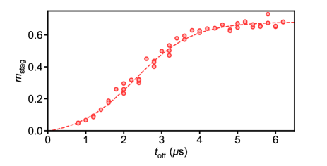
We now discuss the long-term stability of the machine. We do this analysis on the $8\times 8$ array by measuring the growth of antiferromagnetic ordering $m_{\rm{stag}}$ throughout the sweep. The results are presented in Fig. 12. Each point represents a measurement, with $\sim 300$ snapshots recorded over approximately 20 minutes, giving a standard error on the mean which is smaller than the marker size. We repeat the full curve several times over a duration of about 15 hours and observe a spread of $m_{\rm{stag}}$ throughout the sweep. This is due to long-term instabilities of the experimental machine. These are mainly drifts in beam pointing and power of the Rydberg excitation lasers, which slightly change the path of the sweep in the phase diagram, thus affecting the quality of the prepared antiferromagnetic order. The dashed line is a phenomenological fit to the data and is indicative of the mean evolution of $m_{\rm{stag}}$ regarding the long-term drifts of the machine. We use the standard deviation on the fit for the error bars shown on the final points in Fig. 2c,d and Fig. 4b.

Figure 12: Long-term stability of the growth of antiferromagnetic ordering on the $8\times 8$ array. We show several measurements for the same parameters, realised typically over 10 hours. We observe a dispersion of the measurements due to long-term drift of the machine. The dashed line is a phenomenological fit to the data. The standard error on the mean is smaller than symbol size.

.3.5 Growth of antiferromagnetic order

Figure 13: Growth of antiferromagnetic ordering on a $10\times 10$ array during the sweep. Maps of the connected correlations $C_{kl}$ and histograms of the staggered magnetisation for different times $t_{\rm off}$, defined in Fig. 2. The upper (lower) halfs of the plots show experimental (MPS) results.

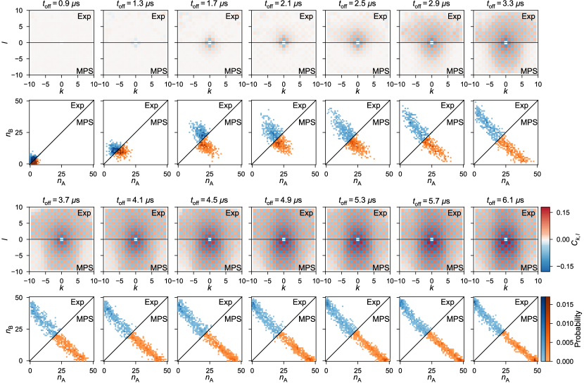
To further compare the MPS calculations to the experimental results we use the snapshot technique, described in Sec. .2.2, to plot the connected correlation maps and the $m_{\rm{stag}}$ histograms for each time step in the sweep on the $10\times 10$ array. These are shown in Fig. 13. The $C_{k,l}$ maps show that the correlations are beginning to develop between 1.3 and 1.7 $\mu$s, and are growing from nearest-neighbour across the array. By 3.8 $\mu$s the expected correlation pattern is filling the entire array, and from then on the strength of the correlations continues to increase. The corresponding $m_{\rm{stag}}$ histograms show the growth in the number of Rydberg excitations as the distribution of points moves from $\sim(0,0)$ to higher values of $n_{\rm{A}}+n_{\rm{B}}$. As the correlations begin to grow across the array we can see the distribution of points stretching along the diagonal and after $3.8~{}\mu$s points start to conglomerate around the corners $(N/2,0)$ and $(0,N/2)$. The MPS results show qualitative agreement throughout the sweep for both observables, with slight differences appearing at times which correspond to disagreements in Fig. 9. This verifies that the dynamical evolution of the atomic system is well approximated by the MPS calculations, including known uncertainties, for all observables. This confirms that we understand and have good control over our platform.

.4 Quantum real-time evolution versus classical equilibrium

In this section we give details on the comparison between the quantum real-time evolution and a classical equilibrium description. We also show that the real-time evolution from MPS simulations does not thermalise and cannot be described by a classical equilibrium distribution, similar to the results for the experiment presented in the main text.

.4.1 Extracting a classical temperature

For a comparison with the classical Hamiltonian (${\Omega=0}$)

$$H_{\text{class}}[\delta]=\sum_{i<j}U_{ij}n_{i}n_{j}-\sum_{i}\hbar\delta_{i}n_{i}\,,$$ (5)

with ${n_{i}\in\{0,1\}}$, we perform Metropolis Monte Carlo simulations with single spin flip updates. Results are averaged over 500 individually equilibrated samples of random atom positions. We take interactions up to a Euclidean distance of $5.2a$, or couplings $U_{ij}\gtrapprox 9.9\times 10^{-5}$ MHz into account. Note that interactions up to a Euclidean distance of $3.3a$, or $U_{ij}\gtrapprox 1.5\times 10^{-3}$ MHz produce nearly identical behaviour on the scales considered here. The $\delta_{i}$ are chosen to reflect the experimental setup, shown in Fig. 10d.

To assign a hypothetical temperature $T_{\rm hyp}$ to the dynamical state of the quantum system, we compute the classical energy for the instantaneous state $\left|\Psi(t_{\text{off}})\right\rangle$,

$$E_{\rm class}(t_{\rm off})=\left\langle\Psi(t_{\rm off})|H_{\rm class}\left[\delta(t_{\rm off})\right]|\Psi(t_{\rm off})\right\rangle$$ (6)

from the corresponding classical Hamiltonian in Eq. (5). Since we do not measure the atom positions for each individual experimental snapshot, we assign the interactions $U_{ij}=U_{\rm nnb}/(r_{ij}/a)^{6}$ to compute $E_{\rm class}$, where $U_{\rm nnb}$ is the atom-position disorder averaged nearest-neighbour interaction (see Fig. 10f). Using classical Monte Carlo we then estimate the classical thermodynamic partition function and compute the energy expectation value for the same classical Hamiltonian for a temperature $T$

$$E_{\rm class}^{\mathrm{MC}}(T)=\sum_{c}H_{\rm class}(c)\,{\rm e}^{-\beta H_{\rm class}(c)}/Z\ ,$$ (7)

where we sum over all classical spin configurations $c$ and have defined $\beta=1/\left(k_{\rm{B}}T\right)$ and $Z=\sum_{c}{\rm e}^{-\beta H_{\rm class}(c)}$. The hypothetical temperature $T_{\rm hyp}(t_{\rm off})$ during the sweep is then computed by matching

$$E_{\text{class}}(t_{\rm off})\equiv E_{\text{class}}^{\mathrm{MC}}(T_{\rm hyp}(t_{\rm off})),$$ (8)

as illustrated in Fig. 14.

Figure 14: Assigning a classical temperature. Classical energy density for the instantaneous state $\left|\Psi(t_{\rm off})\right\rangle$ of the experiment during the last part of the state preparation protocol (left panel), and for the corresponding classical equilibrium system versus temperature $T$ (right panel). Here, $\delta=\delta_{f}$ for all datasets. We assign a hypothetical temperature $T_{\rm hyp}$ at each time $t_{\rm off}$ by matching the classical energy, as illustrated by the red line. In the right panel, $T_{c}$ denotes the critical temperature in the thermodynamic limit $N\rightarrow\infty$.

Figure 15: Evolution of the hypothetical temperature. a, Programmed state preparation protocol and b, corresponding hypothetical temperature $T_{\rm hyp}(t_{\rm off})$ during the sweep for different system sizes. The dashed line shows the classical critical temperature $T_{\rm c}$ for an infinite system with disorder averaged $U/\hbar=2\pi\times 1.86\ \rm{MHz}$ for $\delta_{\rm f}=2\pi\times 2\ \rm{MHz}$.

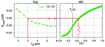
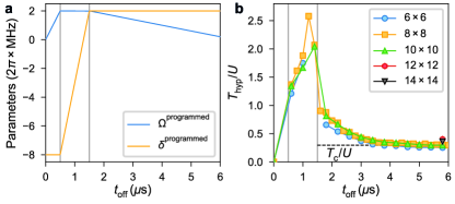
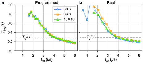
In Fig. 15 we show $T_{\rm hyp}$ during the experimental state preparation process for different system sizes. At $t=0$ the system is in the ground state of $H_{\rm class}$ with $T_{\rm hyp}=0$, since we only consider arrays without any vacancies, and all atoms are in their ground state. During the first parts of the protocol where $\Omega$ is turned on and $\delta$ is increased to its final value, the hypothetical temperature strongly increases. This increase is mainly related to $H_{\rm class}$ not fully describing the quantum driving Hamiltonian $H_{\rm Ryd}$.

During the ramp-down process ($t_{\rm off}>1.5\ \mu\rm{s}$, $\delta=\delta_{\text{f}}$) the boundary to the AF phase is crossed, and we observe a strong “cooling” of the system. At the end of the sweep, we reach very low hypothetical temperatures close to or even below the infinite system size critical temperature $T_{c}$ (see following subsection). The finite temperature at the end of the sweep reflects that the state preparation is not perfectly adiabatic with the durations possible in the experiment.

.4.2 Classical critical temperature

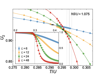
To provide a natural scale for $T_{\rm hyp}$ we compute the critical temperature for the Hamiltonian parameters at the end of the considered sweep ($\Omega=0$), which is defined as the temperature below which the classical system is ordered in the thermodynamic limit. The critical temperature ${T_{c}/U=0.298(1)}$ is extracted from the finite size extrapolation of the Binder cumulant ${U_{2}=\frac{3}{2}\left(1-\langle m_{\text{stag}}^{4}\rangle/3\langle m_{\text{stag}}^{2}\rangle^{2}\right)}$ crossing points as presented in Fig. 16 Binder (1981). Simulations to obtain the Binder cumulant have been performed for systems with homogeneous $\hbar\delta/U=1.075$ (corresponding to $\delta_{f}=2\pi\times 2\ \rm{MHz}$), again using 500 samples of random atom positions with an average nearest neighbour interaction $U/h=U_{\rm nnb}/h=2\pi\times 1.86\ \rm{MHz}$, a Euclidean interaction range of $5.2a$ and periodic boundaries. Note that the scale $T_{c}$, which is only well defined in the infinite-size system, is provided as a reference, but does not preclude the emergence of long range order in finite size systems as observed.

Figure 16: Calculating the critical temperature. The Binder cumulant $U_{2}$ and its ($L$, 2$L$) crossing points (black markers) for different linear system dimensions $L$, which allow to estimate the critical temperature in the thermodynamic limit. The solid (dotted) grey lines indicate the finite size extrapolated $T_{c}$ and its standard error.

.4.3 MPS time evolution versus classical equilibrium

Figure 17: Classical versus quantum state preparation. Distribution of the largest Néel cluster sizes $s_{\rm max}$ during (left panel) and at the end (right panel) of the time evolution from MPS simulations (blue) compared to the classical equilibrium results (yellow) on a $10\times 10$ square lattice. a, Simulation in the setup without including any experimental imperfections. b, Simulation including the known experimental imperfections.

Figure 18: Hypothetical temperature evolution for MPS. $T_{\rm hyp}(t_{\rm off})$ for the MPS simulations during the final part of the state preparation protocol. Different symbols/colours show different system sizes. The panels show MPS simulations a, without, and b with experimental imperfections.

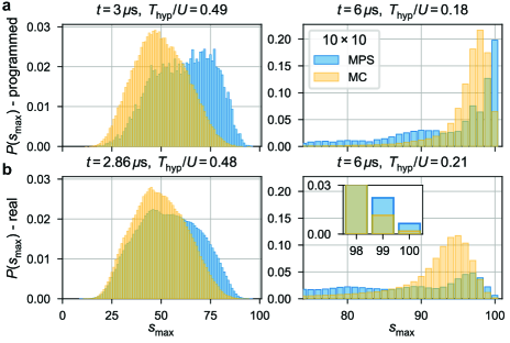
We show in Fig. 3 in the main text, that the distribution of AF domain sizes during the experimental time evolution is strikingly different from a classical equilibrium distribution with an assigned hypothetical temperature $T_{\rm hyp}$. Here, we support this result with an identical analysis for corresponding MPS simulations. We compare the distributions from MPS time evolutions to the corresponding classical equilibrium distributions from MC simulations for both the programmed setup, see Fig. 17a, and the real setup, including experimental imperfections, see Fig. 17b. For intermediate times, shortly after entering the AFM dome (left panels), we observe a similar behaviour as in the experiment for both setups, where the distribution of the MPS simulations is generally shifted towards larger cluster sizes $s_{\rm max}$ compared to the classical distribution. At the end of the sweep (right panels) we still observe that the simulations are not thermalised, since the MPS distributions are not matched by the classical equilibrium ones. Also, the probability of creating Néel states is enhanced compared to the classical distribution, as was observed in the experiment. This effect is very strong in the programmed case, indicating that with experimental improvements we will gain in ground state preparation fidelity.

In Fig. 18, we show the evolution of $T_{\rm hyp}$ for the MPS simulations during the final part of the state preparation protocol for systems with up to $10\times 10$ atoms for both protocols (programmed, real). Similar to the experiment, we observe a strong cooling of the system. At the end of the sweep, we observe that the extracted temperatures from the MPS simulations are somewhat lower than the ones from the experiment, for both the programmed and real cases, pointing to possible further imperfections not yet taken into account.

To conclude one might wonder why the high probability of finding Néel states in the right panel of Fig. 17a does not translate into a substantially lower hypothetical temperature $T_{\rm hyp}$ in the left panel of Fig. 18. The main reason is the temperature dependence of the specific heat of the equilibrium system. In the gapped AF phase the specific heat is exponentially suppressed at low temperature $C(T)\sim\exp(-U/\mathrm{k_{B}}T)$ Onsager (1944). On the other hand the excess energy $\Delta E\equiv E_{\text{class}}-E_{\text{class}}^{\mathrm{GS}}$ is related to the integral of $C(T)$:

$$\Delta E=\int_{0}^{T}C(T^{\prime})dT^{\prime}\ .$$

Combining the two formulas, we infer that $T\sim 1/\log(1/\Delta E)$, i.e. the matching temperature tends to zero only logarithmically slowly with $\Delta E$ going to zero.

.5 Triangular geometries

In this section we consider the peculiarity of the finite-sized triangular array, leading to the observed reduction in the $m_{\rm stag}$ histogram observed for the $2/3$ phase. We also compare classical equilibrium calculations to experimental results on the triangular lattice.

.5.1 Triangular $2/3$ plateau

Figure 19: 2/3 $m_{\rm stag}$ histogram for finite clusters. MC results for a 108-site triangular cluster in the $2/3$ plateau with $\hbar\delta/U=4$ and temperature $T/U=0.1$. a, The real space Rydberg density $n_{i}$ shows that the outermost shell becomes fully populated at low temperature, as also illustrated in the inset which shows the Rydberg density at the edge. b, The corresponding sublattice magnetisation histogram does not reach its full potential width (outer hexagon), since the edge sites cannot participate in the formation of the $2/3$-filling states. The dashed hexagon shows the maximal extend for the histogram when only the sites of the system without the edge are considered.

Figure 20: Quantum real-time evolution versus classical equilibrium on the triangular lattice. a, b, The distribution of the triangular order parameter $m_{\rm stag}$ at the end of the state preparation protocols entering the $1/3$ (a) and $2/3$ (b) regimes. c, Distribution of $m_{\rm stag}$ for a $10\times 10$ square lattice at the end of the sweep entering the AF phase, as a comparison. In all panels, the blue (yellow) bars show experimental (corresponding classical) results. The dashed line in b shows the maximal value of $m_{\rm stag}$ in the $2/3$ regime induced by the cluster boundaries.

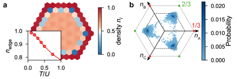
The edge of the finite-sized clusters can have an impact on the achievable ground states, which might differ from the ones expected from the corresponding bulk phase diagram. In particular, the edge sites have fewer direct neighbours than the bulk sites and, hence, they can be excited to Rydberg states at lower $\delta/U$. For the results in this paper, this effect is particularly important for the $2/3$ phase on the triangular clusters, as we will now discuss.

In Fig. 19 we show MC results for a fixed $\hbar\delta/U=4$ in the $2/3$-filling regime at low temperature $T/U=0.1$. It is clearly visible in the Rydberg density $n_{i}$, that the edge sites become completely filled with Rydberg states in the ground state $T\rightarrow 0$. In particular, the Rydberg density on the edge $n_{\rm edge}$ approaches one when the temperature is reduced, see inset in Fig. 19a. Therefore, only the atoms in the bulk can take part in the formation of the $2/3$-filled states, and the maximal order parameter is reduced. This can be directly observed in the sublattice magnetisation histogram, see Fig. 19b, which shows that the position of the three peaks defining the $2/3$ phase do not reach their maximal possible value at the edge of the outer hexagon. Instead, they are bounded by the dashed hexagon, which shows the maximal extend of the histogram for the bulk system. The reduction of the maximal radius is rather large, since it scales with the number of sites on the boundary. In particular, for the here shown 108-site cluster, the boundary consists of 33 sites, leading to $\sim 30\ \%$ reduction of the maximal radius in the histogram. This effect isn’t observed in the $1/3$ regime as $\delta_{f}$ is small enough that the boundary sites also obey the AF ordering.

.5.2 Time evolution vs classical equilibrium on the triangular lattice

Here, we demonstrate that on the triangular lattice the experimental state preparation protocol, again, cannot be reproduced by a classical equilibrium distribution. In Fig. 20a, b we show the experimentally obtained distribution of the order parameter, $m_{\rm stag}$, at the end of the sweep preparing the (a) $1/3$ and (b) $2/3$ phases for the 108 atom array, and compare them to the corresponding classical distribution with hypothetical classical temperature $T_{\rm hyp}$, assigned as described in Sec. .4.1. The experimental distribution is centred at substantially larger values of $m_{\rm stag}$, demonstrating an increased probability of finding highly ordered states compared to a corresponding classical annealing. In Fig. 20c we show, as a comparison, the distribution of $m_{\rm stag}$ for a $10\times 10$ square lattice at the end of the sweep preparing the AF phase, which shows similar, but enhanced, features.

References

- Georgescu et al. (2014) I. M. Georgescu, S. Ashhab, and F. Nori, Quantum simulation, Rev. Mod. Phys. 86, 153 (2014).
- Blatt and Roos (2012) R. Blatt and C. F. Roos, Quantum simulations with trapped ions, Nat. Phys. 8, 277 (2012).
- Monroe et al. (2020) C. Monroe, W. C. Campbell, L.-M. Duan, Z.-X. Gong, A. V. Gorshkov, P. Hess, R. Islam, K. Kim, N. Linke, G. Pagano, P. Richerme, C. Senko, and N. Y. Yao, Programmable Quantum Simulations of Spin Systems with Trapped Ions, arXiv:1912.07845 (2020).
- Gärttner et al. (2017) M. Gärttner, J. G. Bohnet, A. Safavi-Naini, M. L. Wall, J. J. Bollinger, and A. M. Rey, Measuring out-of-time-order correlations and multiple quantum spectra in a trapped-ion quantum magnet, Nat. Phys. 13, 781 (2017).
- Song et al. (2017) C. Song, K. Xu, W. Liu, C.-p. Yang, S.-B. Zheng, H. Deng, Q. Xie, K. Huang, Q. Guo, L. Zhang, P. Zhang, D. Xu, D. Zheng, X. Zhu, H. Wang, Y.-A. Chen, C.-Y. Lu, S. Han, and J.-W. Pan, 10-Qubit Entanglement and Parallel Logic Operations with a Superconducting Circuit, Phys. Rev. Lett. 119, 180511 (2017).
- King et al. (2018) A. D. King, J. Carrasquilla, J. Raymond, I. Ozfidan, E. Andriyash, A. Berkley, M. Reis, T. Lanting, R. Harris, F. Altomare, K. Boothby, P. I. Bunyk, C. Enderud, A. Fréchette, E. Hoskinson, N. Ladizinsky, T. Oh, G. Poulin-Lamarre, C. Rich, Y. Sato, A. Y. Smirnov, L. J. Swenson, M. H. Volkmann, J. Whittaker, J. Yao, E. Ladizinsky, M. W. Johnson, J. Hilton, and M. H. Amin, Observation of topological phenomena in a programmable lattice of 1,800 qubits, Nature 560, 456 (2018).
- Kjaergaard et al. (2020) M. Kjaergaard, M. E. Schwartz, J. Braumüller, P. Krantz, J. I.-J. Wang, S. Gustavsson, and W. D. Oliver, Superconducting Qubits: Current State of Play, Annu. Rev. Condens. Matter Phys 11, 369 (2020).
- Bloch et al. (2008) I. Bloch, J. Dalibard, and W. Zwerger, Many-body physics with ultracold gases, Rev. Mod. Phys. 80, 885 (2008).
- Bloch et al. (2012) I. Bloch, J. Dalibard, and S. Nascimbène, Quantum simulations with ultracold quantum gases, Nat. Phys. 8, 267 (2012).
- Gross and Bloch (2017) C. Gross and I. Bloch, Quantum simulations with ultracold atoms in optical lattices, Science 357, 995 (2017).
- Browaeys and Lahaye (2020) A. Browaeys and T. Lahaye, Many-body physics with individually controlled Rydberg atoms., Nat. Phys. 16, 132 (2020).
- Yan et al. (2013) B. Yan, S. A. Moses, B. Gadway, J. P. Covey, K. R. A. Hazzard, A. M. Rey, D. S. Jin, and J. Ye, Observation of dipolar spin-exchange interactions with lattice-confined polar molecules, Nature 501, 521 (2013).
- Zhou et al. (2011) Y. L. Zhou, M. Ortner, and P. Rabl, Long-range and frustrated spin-spin interactions in crystals of cold polar molecules, Phys. Rev. A 84, 052332 (2011).
- Bernien et al. (2017) H. Bernien, S. Schwartz, A. Keesling, H. Levine, A. Omran, H. Pichler, S. Choi, A. S. Zibrov, M. Endres, M. Greiner, V. Vuletić, and M. D. Lukin, Probing many-body dynamics on a 51-atom quantum simulator, Nature 551, 579 (2017).
- Keesling et al. (2019) A. Keesling, A. Omran, H. Levine, H. Bernien, H. Pichler, S. Choi, R. Samajdar, S. Schwartz, P. Silvi, S. Sachdev, P. Zoller, M. Endres, M. Greiner, V. Vuletić, and M. D. Lukin, Quantum Kibble–Zurek mechanism and critical dynamics on a programmable Rydberg simulator, Nature 568, 207 (2019).
- Lienhard et al. (2018) V. Lienhard, S. de Léséleuc, D. Barredo, T. Lahaye, A. Browaeys, M. Schuler, L.-P. Henry, and A. M. Läuchli, Observing the Space- and Time-Dependent Growth of Correlations in Dynamically Tuned Synthetic Ising Antiferromagnets, Phys. Rev. X 8, 021070 (2018).
- Levine et al. (2019) H. Levine, A. Keesling, G. Semeghini, A. Omran, T. T. Wang, S. Ebadi, H. Bernien, M. Greiner, V. Vuletić, H. Pichler, and M. D. Lukin, Parallel Implementation of High-Fidelity Multiqubit Gates with Neutral Atoms, Phys. Rev. Lett. 123, 170503 (2019).
- Omran et al. (2019) A. Omran, H. Levine, A. Keesling, G. Semeghini, T. T. Wang, S. Ebadi, H. Bernien, A. S. Zibrov, H. Pichler, S. Choi, J. Cui, M. Rossignolo, P. Rembold, S. Montangero, T. Calarco, M. Endres, M. Greiner, V. Vuletić, and M. D. Lukin, Generation and manipulation of Schrödinger cat states in Rydberg atom arrays, Science 365, 570 (2019).
- Madjarov et al. (2020) I. S. Madjarov, J. P. Covey, A. L. Shaw, J. Choi, A. Kale, A. Cooper, H. Pichler, V. Schkolnik, J. R. Williams, and M. Endres, High-fidelity entanglement and detection of alkaline-earth Rydberg atoms, Nat. Phys. 16, 857 (2020).
- Schauß et al. (2015) P. Schauß, J. Zeiher, T. Fukuhara, S. Hild, M. Cheneau, T. Macrì, T. Pohl, I. Bloch, and C. Gross, Crystallization in Ising quantum magnets, Science 347, 1455 (2015).
- Guardado-Sanchez et al. (2018) E. Guardado-Sanchez, P. T. Brown, D. Mitra, T. Devakul, D. A. Huse, P. Schauß, and W. S. Bakr, Probing the Quench Dynamics of Antiferromagnetic Correlations in a 2D Quantum Ising Spin System, Phys. Rev. X 8, 021069 (2018).
- Song et al. (2020) Y. Song, M. Kim, H. Hwang, W. Lee, and J. Ahn, Quantum annealing of Cayley-tree Ising spins at small scales, arXiv:2011.01653 (2020).
- Wannier (1950) G. H. Wannier, Antiferromagnetism. The Triangular Ising Net, Phys. Rev. 79, 357 (1950).
- Jaksch et al. (2000) D. Jaksch, J. I. Cirac, P. Zoller, S. L. Rolston, R. Côté, and M. D. Lukin, Fast Quantum Gates for Neutral Atoms, Phys. Rev. Lett. 85, 2208 (2000).
- Schymik et al. (2020) K.-N. Schymik, V. Lienhard, D. Barredo, P. Scholl, H. Williams, A. Browaeys, and T. Lahaye, Enhanced atom-by-atom assembly of arbitrary tweezer arrays, Phys. Rev. A 102, 063107 (2020).
- Levine et al. (2018) H. Levine, A. Keesling, A. Omran, H. Bernien, S. Schwartz, A. S. Zibrov, M. Endres, M. Greiner, V. Vuletić, and M. D. Lukin, High-Fidelity Control and Entanglement of Rydberg-Atom Qubits, Phys. Rev. Lett. 121, 123603 (2018).
- Janke and Villanova (1997) W. Janke and R. Villanova, Three-dimensional 3-state Potts model revisited with new techniques, Nucl. Phys. B 489, 679 (1997).
- Laumann et al. (2012) C. R. Laumann, R. Moessner, A. Scardicchio, and S. L. Sondhi, Quantum Adiabatic Algorithm and Scaling of Gaps at First-Order Quantum Phase Transitions, Phys. Rev. Lett. 109, 030502 (2012).
- Fey et al. (2019) S. Fey, S. C. Kapfer, and K. P. Schmidt, Quantum Criticality of Two-Dimensional Quantum Magnets with Long-Range Interactions, Phys. Rev. Lett. 122, 017203 (2019).
- Samajdar et al. (2020) R. Samajdar, W. W. Ho, H. Pichler, M. D. Lukin, and S. Sachdev, Complex Density Wave Orders and Quantum Phase Transitions in a Model of Square-Lattice Rydberg Atom Arrays, Phys. Rev. Lett. 124, 103601 (2020).
- Note (1) The residual anisotropy observed is due to the finite size of the excitation beams, which is comparable to the width of the array (m).
- Stoli and Domb (1979) E. Stoli and C. Domb, Shape and size of two-dimensional percolation clusters with and without correlations, J. Phys. A 12, 1843 (1979).
- Kim et al. (2018) H. Kim, Y. Park, K. Kim, H.-S. Sim, and J. Ahn, Detailed Balance of Thermalization Dynamics in Rydberg-Atom Quantum Simulators, Phys. Rev. Lett. 120, 180502 (2018).
- Note (2) One could also use other observables to match a hypothetical temperature, but since temperature is the variable conjugate to the energy in thermodynamics, it is the most natural choice.
- Pichler et al. (2018) H. Pichler, S.-T. Wang, L. Zhou, S. Choi, and M. D. Lukin, Quantum Optimization for Maximum Independent Set Using Rydberg Atom Arrays, arXiv:1808.10816 (2018).
- Henriet (2020) L. Henriet, Robustness to spontaneous emission of a variational quantum algorithm, Phys. Rev. A 101, 012335 (2020).
- Serret et al. (2020) M. F. Serret, B. Marchand, and T. Ayral, Solving optimization problems with Rydberg analog quantum computers: Realistic requirements for quantum advantage using noisy simulation and classical benchmarks, Phys. Rev. A 102, 052617 (2020).
- Villain et al. (1980) J. Villain, R. Bidaux, J.-P. Carton, and R. Conte, Order as an effect of disorder, J. Phys. France 41, 1263 (1980).
- Moessner et al. (2000) R. Moessner, S. L. Sondhi, and P. Chandra, Two-Dimensional Periodic Frustrated Ising Models in a Transverse Field, Phys. Rev. Lett. 84, 4457 (2000).
- Moessner and Sondhi (2001) R. Moessner and S. L. Sondhi, Ising models of quantum frustration, Phys. Rev. B 63, 224401 (2001).
- Isakov and Moessner (2003) S. V. Isakov and R. Moessner, Interplay of quantum and thermal fluctuations in a frustrated magnet, Phys. Rev. B 68, 104409 (2003).
- Koziol et al. (2019) J. Koziol, S. Fey, S. C. Kapfer, and K. P. Schmidt, Quantum criticality of the transverse-field Ising model with long-range interactions on triangular-lattice cylinders, Phys. Rev. B 100, 144411 (2019).
- Madjarov et al. (2019) I. S. Madjarov, A. Cooper, A. L. Shaw, J. P. Covey, V. Schkolnik, T. H. Yoon, J. R. Williams, and M. Endres, An Atomic-Array Optical Clock with Single-Atom Readout, Phys. Rev. X 9, 041052 (2019).
- Norcia et al. (2019) M. A. Norcia, A. W. Young, W. J. Eckner, E. Oelker, J. Ye, and A. M. Kaufman, Seconds-scale coherence on an optical clock transition in a tweezer array, Science 366, 93 (2019).
- Saffman et al. (2010) M. Saffman, T. G. Walker, and K. Mølmer, Quantum information with Rydberg atoms, Rev. Mod. Phys. 82, 2313 (2010).
- Henriet et al. (2020) L. Henriet, L. Béguin, A. Signoles, T. Lahaye, A. Browaeys, G.-O. Reymond, and C. Jurczak, Quantum computing with neutral atoms, Quantum 4, 327 (2020).
- Morgado and Whitlock (2020) M. Morgado and S. Whitlock, Quantum simulation and computing with Rydberg qubits, arXiv:2011.03031 (2020).
- Barredo et al. (2018) D. Barredo, V. Lienhard, S. de Léséleuc, T. Lahaye, and A. Browaeys, Synthetic three-dimensional atomic structures assembled atom by atom, Nature 561, 79 (2018).
- de Léséleuc et al. (2018) S. de Léséleuc, D. Barredo, V. Lienhard, A. Browaeys, and T. Lahaye, Analysis of imperfections in the coherent optical excitation of single atoms to Rydberg states, Phys. Rev. A 97, 053803 (2018).
- Schollwöck (2011) U. Schollwöck, The density-matrix renormalization group in the age of matrix product states, Ann. Phys. (NY) 326, 96 (2011).
- Paeckel et al. (2019) S. Paeckel, T. Köhler, A. Swoboda, S. R. Manmana, U. Schollwöck, and C. Hubig, Time-evolution methods for matrix-product states, Ann. Phys. (NY) 411, 167998 (2019).
- Stoudenmire and White (2012) E. M. Stoudenmire and S. R. White, Studying Two-Dimensional Systems with the Density Matrix Renormalization Group, Annu. Rev. Condens. Matter Phys 3, 111 (2012).
- Eisert et al. (2010) J. Eisert, M. Cramer, and M. B. Plenio, Colloquium: Area laws for the entanglement entropy, Rev. Mod. Phys. 82, 277 (2010).
- Haegeman et al. (2011) J. Haegeman, J. I. Cirac, T. J. Osborne, I. Pižorn, H. Verschelde, and F. Verstraete, Time-Dependent Variational Principle for Quantum Lattices, Phys. Rev. Lett. 107, 070601 (2011).
- Haegeman et al. (2016) J. Haegeman, C. Lubich, I. Oseledets, B. Vandereycken, and F. Verstraete, Unifying time evolution and optimization with matrix product states, Phys. Rev. B 94, 165116 (2016).
- Hauschild and Pollmann (2018) J. Hauschild and F. Pollmann, Efficient numerical simulations with Tensor Networks: Tensor Network Python (TeNPy), SciPost Phys. Lect. Notes , 5 (2018).
- Stoudenmire and White (2010) E. M. Stoudenmire and S. R. White, Minimally entangled typical thermal state algorithms, New J. Phys 12, 055026 (2010).
- Marcuzzi et al. (2017) M. Marcuzzi, J. Minář, D. Barredo, S. de Léséleuc, H. Labuhn, T. Lahaye, A. Browaeys, E. Levi, and I. Lesanovsky, Facilitation Dynamics and Localization Phenomena in Rydberg Lattice Gases with Position Disorder, Phys. Rev. Lett. 118, 063606 (2017).
- Binder (1981) K. Binder, Finite size scaling analysis of ising model block distribution functions, Z. Phys. B: Condens. Matter 43, 119 (1981).
- Onsager (1944) L. Onsager, Crystal Statistics. I. A Two-Dimensional Model with an Order-Disorder Transition, Phys. Rev. 65, 117 (1944).