Deep Deterministic Policy Gradient for Relay Selection and Power Allocation in Cooperative Communication Network

Abstract

Perfect channel state information (CSI) is usually required when considering relay selection and power allocation in cooperative communication. However, it is difficult to get an accurate CSI in practical situations. In this letter, we study the outage probability minimizing problem based on optimizing relay selection and transmission power. We propose a prioritized experience replay aided deep deterministic policy gradient learning framework, which can find an optimal solution by dealing with continuous action space, without any prior knowledge of CSI. Simulation results reveal that our approach outperforms reinforcement learning based methods in existing literatures, and improves the communication success rate by about $4\%$.

I Introduction

In recent years, cooperative communication has been paid much attention, for it can help realizing resource collaboration between different nodes and obtaining diversified benefits in multi-user scenario [1]. In cooperative communication, an outage occurs when the received signal-to-noise ratio (SNR) falls below a certain threshold [2], and outage probability is usually used as a metric to measure the Quality-of-Service (QoS) of communication system. In order to minimize outage probability and improve QoS, it is intuitive to optimize relay selection and power allocation schemes. Traditional methods usually establish a probabilistic model based on the distribution assumption of channel uncertainty [3, 4, 5], and then design relay or power optimizing scheme. It should be noted that assuming an exact channel state information (CSI) is usually impractical because of the inevitable noise. Therefore, artificial assumptions about channel state distribution may bring estimation bias and mislead the final decision.

Reinforcement learning (RL) is one of the three paradigms of machine learning. RL methods use an agent, which can be taken as an intelligent robot, to interact with and learn from the communication environment, and thus do not need any prior knowledge or assumptions about the environment. In addition, different from other machine learning methods, RL methods do not require data sets, because all the training data is obtained through continuous interaction [6]. After online data collecting and offline learning, the well-trained network models can be implanted into corresponding equipments for practical use.

To address the aforementioned issue in cooperative communication, several methods have been proposed with the help of RL, by using which optimizing strategy can be directly learned from original communication environment. Khan et al. used SARSA-$\lambda$ algorithm to make an adaptive power allocation [7]. In [8] and [9], Q-learning algorithm was employed to help power control and relay selection, respectively. In [10, 11, 12], the authors developed deep Q network (DQN), which is a combination of RL and deep neural network (DNN), for relay-aided communication. Further, [13] introduced convolutional neural network (CNN) to study relay features in several previous time slots, then the output of CNN is used for value estimation in DQN. Although such modification obtained improvement in system performance, the computational complexity increased considerably. On the other hand, however, none of above studies have successfully addressed power allocation problems with continuous action space. These methods have to set several optional power levels within the given power range for agent to choose from, and thus the final scheme is usually not optimal.

Motivated by this, in this letter, we propose a prioritized experience replay aided deep deterministic policy gradient (PER-DDPG) learning framework for the outage probability minimization problem. The proposed method performs efficient experience learning, and realizes precise control of continuous action by performing gradient operation directly on the action policy, with which the agent can optimize its action policy for discretized relay selection and continuous power allocation.

II System Model and Problem Formulation

As shown in Fig. 1, there is an $N_{S}$-antenna source $S$, an $N_{D}$-antenna destination $D$, and a group of single-antenna relays $R=\{R_{1},R_{2},\dots,R_{K}\}$ in the two-hop wireless relay network. Suppose the source is far from the destination, and it does not have the direct link to destination. Therefore, the relay which uses amplify-and-forward (AF) protocol to process the received signal, is needed to help communication.

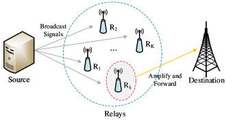
Figure 1: Cooperative relay network.

We consider a half-duplex signaling mode because of equipment limitation. The source selects only one relay and orthogonal channels are used, in order to achieve full set gain and avoid mutual interference. Therefore, the communication from source $S$ to destination $D$ via the selected relay $R_{k}$ will take two time slots.

In the first time slot, the source broadcasts its signal, then all candidate relays listen to this transmission. The received signal at $R_{k}$ can be written as

$$y_{sk}(t)=\sqrt{P_{s}}\boldsymbol{w}_{s}^{\dagger}\boldsymbol{h}_{sk}(t)x(t)+n_{k}(t),$$ (1)

where $P_{s}\in[0,P_{max}]$ represents the transmission power at source, $x(t)$ represents data symbol. $\boldsymbol{h}_{sk}$ represents channel vector between source and relay $R_{k}$, where each element is a complex Gaussian random variable with zero mean and variance $\sigma_{sk}^{2}$, and $n_{k}$ is the complex Gaussian noise with variance $\sigma_{n}^{2}$ at relay. $\boldsymbol{w}_{s}^{\dagger}=\boldsymbol{h}_{sk}/\|\boldsymbol{h}_{sk}\|$ is the normalized beamforming vector using principles of maximal ratio transmission, where $\dagger$ denotes conjugate transpose operation.

In the second time slot, the selected relay amplifies and forwards the detected signal to destination. Then the received signal at destination can be written as

$$\boldsymbol{y}_{kd}(t)=\sqrt{P_{r}}\boldsymbol{h}_{kd}(t)\beta y_{sk}(t)+\boldsymbol{n}_{d}(t),$$ (2)

where $P_{r}\in[0,P_{max}]$ is the transmission power at relay, and similarly, $\boldsymbol{h}_{sk}$ represents channel vector between relay and destination, $\boldsymbol{n}_{d}\sim\mathcal{CN}(\boldsymbol{0},\sigma_{n}^{2}\boldsymbol{I}_{N_{D}})$ is the complex Gaussian noise at destination. By employing maximal ratio combining methods, we multiply signal $\boldsymbol{y}_{kd}$ by a beamforming vector $\boldsymbol{w}_{d}^{\dagger}=\boldsymbol{h}_{kd}/\|\boldsymbol{h}_{kd}\|$, and have

$$x_{kd}(t)=\sqrt{P_{s}P_{r}} \boldsymbol{w}_{d}^{\dagger}\boldsymbol{h}_{kd}(t)\beta\boldsymbol{w}_{s}\boldsymbol{h}_{sk}x(t)+$$ (3)

$$+\sqrt{P_{r}}\boldsymbol{w}_{d}^{\dagger}\boldsymbol{h}_{kd}(t)\beta n_{k}(t)+\boldsymbol{w}_{d}^{\dagger}\boldsymbol{n}_{d}(t),$$

where $\beta^{2}=(P_{s}\|\boldsymbol{h}_{sk}\|^{2}+\sigma^{2}_{n})^{-1}$ is the amplification factor.

Similar to [10, 14], we have the final end-to-end SNR $\varphi_{z}=\varphi_{sk}\varphi_{kd}/(\varphi_{sk}+\varphi_{kd}+1)$ after some manipulations, where $\varphi_{sk}=P_{s}{\|\boldsymbol{h}_{sk}\|}^{2}/\sigma_{n}^{2}$ and $\varphi_{kd}=P_{r}{\|\boldsymbol{h}_{kd}\|}^{2}/\sigma_{n}^{2}$. Then we have the mutual information (MI) between source and destination using unit bandwidth.

$$I=\frac{1}{2}\log_{2}(1+\frac{\varphi_{si}\varphi_{id}}{\varphi_{si}+\varphi_{id}+1}).$$ (4)

We assume that the RL agent has access to CSI in the previous time slot, which can be denoted as $\boldsymbol{h}(t)=\{\boldsymbol{h}_{sk}(t-1),\boldsymbol{h}_{kd}(t-1)\}$. Then we define the following indicator function to represent the outage event.

$$f(t)\triangleq f\big{(}R_{k}(t),P_{s}(t),P_{r}(t);\boldsymbol{h}(t)\big{)}\triangleq\mathbbm{1}_{I<\lambda},$$ (5)

where $\lambda>0$ denotes the outage threshold, and $\mathbbm{1}_{I<\lambda}$ denotes the indicator function which equals to 1 when the inequality $I<\lambda$ is satisfied. Since the expectation of an indicator function can be used to calculate the probability of its original event, we then formulate the optimization problem for minimizing outage probability as follows.

$$\boldsymbol{P}_{1}:\min\limits_{R_{k}(t),P_{s}(t),P_{r}(t)}\mathbb{E}\Bigg{[}\frac{1}{T}\sum\limits_{t=1}^{T}f(t)\Bigg{]}$$ (6)

s.t. $$\textbf{C}_{1}:R_{k}\in\{R_{1},R_{2},\dots,R_{K}\},$$

$$\textbf{C}_{2}:0\leq P_{s},P_{r}\leq P_{max},$$

$$\textbf{C}_{3}:P_{s}+P_{r}\leq P_{max},$$

where $\mathbb{E}[\cdot]$ denotes expectation operation, and our goal is to minimize the average outage probability over $T$ time slots.

III Deep Reinforcement Learning Method

Without acquiring real-time CSI, we turn to RL methods for solutions. In our method, the source node acts as RL agent, and selects a proper relay and sets transmission power according to its observation of historical CSI, then it receives communication result as reward from the environment. In this section, we model this process as a Markov decision process (MDP), and then describe our proposed method.

III-A Markov Decision Process and System Variables

The MDP consists of environment $\mathcal{E}$, state space $\mathcal{S}$, action space $\mathcal{A}$, and reward space $\mathcal{R}$. At each time step $t$, RL agent observes current state $s_{t}\in\mathcal{S}_{t}$, and accordingly selects action $a_{t}\in\mathcal{A}_{t}$. After executing action $a_{t}$, it receives a scalar reward $r_{t}\in\mathcal{R}_{t}$ from the environment $\mathcal{E}$ and observers next state $s_{t+1}$. This process will continue until terminal state is reached. Specifically, components of our system are designed as follows.

• Environment: The environment is a virtual scenario which corresponds to the two-hop cooperative communication system established in section II.

• RL Agent: In our proposed method, the source node is equipped with learning ability, and is considered as RL agent. Note that, any information about the environment is unknown to RL agent at the beginning. Therefore, RL agent needs to act and interact with the environment to obtain experiences for strategy learning.

• System State: Full observation of environment consists of channel states between any two nodes in the previous time slot. Therefore, we consider historical channel state $\boldsymbol{h}(t)$ as system state, which can be denoted as

  $$\mathcal{S}_{t}\triangleq[\boldsymbol{h}_{sk}(t-1),\boldsymbol{h}_{kd}(t-1)],$$ (7)

  where $\boldsymbol{h}_{sk}(t-1)$ represents the set of channel vectors between source and all relays in time slot $t-1$, and similarly $\boldsymbol{h}_{kd}(t-1)$ represents that between all relays and destination. More specifically, in our simulation environment, channel states of adjacent time slots will change according to the following Gaussian Markov block fading autoregressive model [15, 14], which the RL agent has no prior knowledge about.

  $$\boldsymbol{h}_{ij}(t)=\rho\boldsymbol{h}_{ij}(t-1)+\sqrt{1-\rho^{2}}\boldsymbol{e}(t),$$ (8)

  where $\rho$ denotes the normalized channel correlation coefficient, and $\boldsymbol{e}(t)\sim\mathcal{CN}(\boldsymbol{0},\sigma^{2}\boldsymbol{I})$ denotes the error variable and is uncorrelated with $\boldsymbol{h}_{ij}(t)$.

• System Action: In each time slot, RL agent needs to select relay and make power allocation simultaneously. Therefore, our system action can be defined as

  $$\mathcal{A}_{t}\triangleq[a^{R}(t),a^{P_{s}}(t)],$$ (9)

  where $a^{R}(t)\in\{1,2,\dots,K\}$ and $a^{P_{s}}(t)\in[0,P_{max}]$. Note that, the action for $P_{r}(t)$ is omitted, for it can be replace by the subtraction of $P_{max}$ and $P_{s}(t)$.

• Reward Function: In this letter, we consider an extreme case that the only feedback our agent gets is a binary result of successful or unsuccessful communication, which can be denoted as $\mathcal{R}_{t}=\{0,1\}$. Accordingly, we design the following outage-based binary reward function.

  $$r_{t}=r(s_{t},a_{t})\triangleq 1-f\big{(}a^{R}(t),a^{P_{s}}(t);\boldsymbol{h}(t)\big{)}.$$ (10)

The total accumulated reward at time step $t$ can be written as $R_{t}=\sum\nolimits_{i=t}^{T}\gamma^{i-t}r_{i}$, where $T$ denotes total step and $\gamma\in[0,1]$ denotes discount factor. The goal of RL agent is to maximize the expected accumulated reward from each state $s_{t}$.

III-B PER-DDPG Solution

To achieve optimal actions under different states, the action-value function $Q(s_{t},a_{t};\theta)=\mathbb{E}[R_{t}|s_{t},a_{t}]$ is first defined to describe the expected return after selecting action $a_{t}$ in state $s_{t}$, which is controlled by network parameter $\theta$. Then, the optimal action-value function is denoted as $Q^{\ast}(s_{t},a_{t};\theta)=\max_{a_{t}\in\mathcal{A}_{t}}Q(s_{t},a_{t};\theta)$, which obeys Bellman function.

$$Q^{\ast}(s_{t},a_{t};\theta)=\mathbb{E}_{s_{t+1}\sim\mathcal{E}}[r+\gamma\max\limits_{a_{t+1}}Q(s_{t+1},a_{t+1};\theta)],$$ (11)

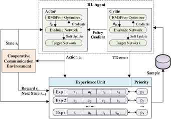
Figure 2: PER-DDPG learning framework.

The utilization of DNN has guaranteed the ability of generalization in terms of action-value estimation. Further, to data-efficiently deal with continuous power action space, we propose a PER-DDPG learning method, whose framework is shown in Fig. 2.

For sampling efficiently, we maintain a prioritized experience buffer $\mathcal{B}$, to store agent’s experience unit $e_{t}=\{s_{t},a_{t},r_{t},s_{t+1}\}$ after each interaction. The priority $p_{t}$ indicates the importance of corresponding unit, and it is intuitive to employ TD error $\delta_{t}$ as a proxy for priority, which specifically shows the difference between current state-action value and its next-step bootstrap estimation. The larger the value, the more RL agent can learn from this experience unit.

When calculating the priority, a small positive constant $\epsilon$ is introduced, i.e. $p_{t}=|\delta_{t}|+\epsilon$, to ensure that each unit has the probability to be sampled even if its TD error is zero. In addition, to correct the bias illustrated in [16], we accordingly employ the following importance-sampling weight

$$w_{i}=\frac{(B_{size}\cdot p_{i})^{-\kappa}}{\max\nolimits_{j<t}w_{j}},$$ (12)

where $B_{size}$ denotes the size of experience buffer, and $\kappa$ is an exponent between 0 and 1.

In terms of RL agent, it consists of two parts, which are called actor and critic, respectively [17]. Further, the agent employs two separate DNNs for both of them, which are known as evaluate network and target network.

Critic: The critic estimates action-value function by employing a DNN with parameter $\theta_{Q}$. During training process, the agent samples a mini-batch of experience units according to experience priority. Similar to other value-based RL methods, the critic tries to minimize the following loss function.

$$L(\theta_{Q})=\mathbb{E}_{e_{t}\sim\mathcal{B}}\Big{[}w_{t}\cdot\delta_{t}^{2}(s_{t},a_{t};\theta_{Q})\Big{]}$$ (13)

with TD error represented as

$$\delta_{t}(s_{t},a_{t};\theta_{Q})=r_{t}+\gamma\max\limits_{a_{t+1}}Q(s_{t+1},a_{t+1};\theta^{-}_{Q})-Q(s_{t},a_{t};\theta_{Q}),$$ (14)

where $\theta^{-}_{Q}$ is a group of old parameters in target network. In order to improve learning stability, old parameters will be soft replaced periodically following $\theta^{-}_{Q}\leftarrow\tau\theta_{Q}+(1-\tau)\theta^{-}_{Q}$ with $\tau\ll 1$. Afterwards, parameters in evaluate network will be updated using RMSProp optimization.

$$\theta_{Q}\leftarrow\theta_{Q}-\eta_{Q}w_{t}\delta_{t}(s_{t};\theta_{Q})\nabla_{\theta_{Q}}Q(s_{t},a_{t};\theta_{Q}),$$ (15)

where $\eta_{Q}$ denotes learning step size for critic.

Actor: The actor is used to learn action policy and perform primitive actions. It maintains a parameterized function $\mu(s;\theta_{\mu})$, which specifies the current policy by deterministically mapping states to specific actions. We define the following performance objective for current action policy.

$$J(\theta_{\mu})=\mathbb{E}_{s_{t}\sim\mathcal{B}}[Q(s_{t},\mu(s_{t};\theta_{\mu});\theta_{Q})].$$ (16)

The gradient of such deterministic policy moves the action policy in the direction of the gradient of action-value function, that is, network parameters $\theta_{\mu}$ will be updated in proportion to $\nabla_{\theta_{\mu}}Q(s_{t},\mu(s_{t};\theta_{\mu});\theta_{Q})$. By using chain rule, it can be divided into two parts as shown below.

$$\nabla_{\theta_{\mu}}J=\mathbb{E}_{s_{t}} \Big{[}\nabla_{\theta_{\mu}}\mu(s_{t};\theta_{\mu})\nabla_{a}Q(s_{t},a_{t};\theta_{Q})|_{a_{t}=\mu(s_{t};\theta_{\mu})}\Big{]},$$ (17)

based on which the actor parameters $\theta_{\mu}$ is updated as follows.

$$\theta_{\mu}\leftarrow\theta_{\mu}-\eta_{\mu}\nabla_{\theta_{\mu}}J,$$ (18)

where similarly $\eta_{\mu}$ denotes learning step size for actor.

Pseudocode of our method can be found in Algorithm 1.

Algorithm 1 PER-DDPG for Relay and Power Optimization

1:  Initialize experience buffer $\mathcal{B}=\varnothing$.

2:  Initialize evaluate network parameters $\theta_{Q}$ and $\theta_{\mu}$.

3:  Initialize target network with $\theta^{-}_{Q}=\theta_{Q}$ and $\theta^{-}_{\mu}=\theta_{\mu}$.

4:  for episode $u=1,2,\dots,u_{max}$ do

5:     Initialize communication environment, get state $s_{1}$.

6:     Initialize a random process $\Delta\mu$ as noise.

7:     for time slot $t=1,2,\dots,t_{max}$ do

8:        Choose action $a_{t}=\mu(s_{t};\theta_{\mu})+\Delta\mu_{t}$ to determine the selected relay and power for transmission.

9:        Execute action $a_{t}$, then receive reward $r_{t}$ and observe next state $s_{t+1}$.

10:        Collect and save current experience $e_{t}$ with initial priority $p_{t}=\max_{i<t}p_{i}$, and then sample a mini-batch of experience units $e_{j}$ according to probability $p(j)=p_{j}^{\alpha}/{\sum\nolimits_{i}p_{i}^{\alpha}}$ with predefined exponent $\alpha$.

11:        Calculate importance-sampling weight and TD error of each experience unit according to (12) and (14).

12:        Minimize the loss of mini-batch in (13), and update evaluate network of critic according to (15).

13:        Calculate the sampled policy gradient in (17), and update evaluate network of actor according to (18).

14:        Update experience priority using $p_{j}=|\delta_{j}|+\epsilon$.

15:        Update parameters of corresponding target networks by $\theta^{-}_{Q}\leftarrow\tau\theta_{Q}+(1-\tau)\theta^{-}_{Q}$ and $\theta^{-}_{\mu}\leftarrow\tau\theta_{\mu}+(1-\tau)\theta^{-}_{\mu}$.

16:     end for

17:  end for

IV Evaluation

In this section, we present implementation details of simulation environment, and demonstrate performance of the proposed method. Similar to the settings in [10], the required outage threshold is set as $\lambda=0.1$, and total maximum power $P_{max}$ for source and relay transmission is 1W. Learning rates for updating critic network and actor network are set as $\eta_{Q}=0.005$ and $\eta_{\mu}=0.001$, respectively. Parameter for soft update is set as $\tau=0.001$. In addition, the size of experience buffer $B_{size}$ is 10000, and mini-batch size which determines numbers of training cases is 128.

Given the lack of knowledge of the underlying channel distribution in actual communication system, we mainly employ random selection and existing RL algorithms as baseline methods. More specifically, since the PER operation can be decoupled from our proposed method, we are able to take original DDPG scheme for comparison. In addition, DQN is a widely used RL method in the field of communication, which we will also take as a baseline method. Note that, DQN can only solve problems with discrete action spaces. Therefore, when using this method, we divide the power into $L$ power levels for the agent to choose from, which can be denoted as $\frac{1}{L}P_{max},\frac{2}{L}P_{max},\dots,P_{max}$.

We first evaluate the training performance of different methods with total training episodes $\mu_{max}=100$. Specifically, we first perform 10 training trials for each method. Then, we select the successful trials among these 10 repetitions, and use solid line to represent the median and shadow region to represent the range of them.

As shown in Fig. 3, the training performance of random selection is poor, while all DRL methods can converge. Before training with our proposed method (orange line) and its another version without handling experience replay (blue line), we both use 10 episodes for RL agent to select randomly and collect enough experience units. We find that, PER-DDPG and original DDPG can finally converge to a similar value. When compared with DQN method (green line), our method can achieve a better result with an improvement of about $4\%$ in average success rate.

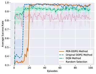
Figure 3: Average success rate with different methods.

For better explanation, we also present the statistic for all successful training trials in Table I, where we analyze the performance of the last 40 episodes (i.e. Episode 61-100, after training curves converge).

TABLE I: Statistic of 10 trials with different methods.

Method	Successful trials	Mean	Standard deviation
PER-DDPG	10	0.969	$1.374*10^{-2}$
Original DDPG	9	0.955	$3.209*10^{-2}$
DQN	10	0.926	$2.003*10^{-2}$
Random	-	0.835	-

We find that with our PER-DDPG method, RL agent can obtain appropriate action policy every time, but there is one record of failure using its original version. What’s more, we observe that although original DDPG trains faster, our PER-DDPG method has smaller standard variance. As vividly depicted in Fig. 3, the fluctuation of PER-DDPG’s training curve is slighter, and the shadow region is smaller. Actually, such failure in using original DDPG is caused by the interplay between the actor and critic updates [18]. The usage of outdated experience unit can lead to a high variance in value estimate, which then misleads policy updates. However, with the help of PER, we realize efficient data sampling, and can achieve better stability during the training process.

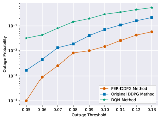
Figure 4: Testing result under different outage thresholds.

In testing process, we evaluate the outage probability of these well-trained DRL models with different threshold requirements. Note that, corresponding to the training process, we preserve all successful trained network models for each method. Then we record the average performance of each method. The testing result is depicted in Fig. 4, where we can obviously find that our PER-DDPG model still has better performance than other models. Although original DDPG method can achieve an average success rate close to that of PER-DDPG method in training stage, due to its larger variance, the results obtained in test process are not good. On the other hand, DQN model always performs worse than model with policy gradient methods, for it can only perform coarse-grained discrete power optimization. From the above, our proposed method can obtain a robust action policy, which can effectively reduce outage probability and be applied to other situations.

V Conclusion

In this letter, we introduce deep deterministic policy gradient into dynamic relay selection and power optimization in a two-hop cooperative relay network, and realize data efficiency with the help of prioritized experience. Unlike traditional studies, our method does not rely on any assumptions about channel distribution, and can effectively deal with optimization variables which have continuous action space. Simulation results reveal that with our PER-DDPG method, the average communication success rate can be increased by about $4\%$ compared to existing RL methods.

References

- [1] F. Zhong, X. Xia, H. Li, and Y. Chen, “Distributed linear convolutional space-time coding for two-hop full-duplex relay 2x2x2 cooperative communication networks,” IEEE Transactions on Wireless Communications, vol. 17, no. 5, pp. 2857–2868, May 2018.
- [2] Y. Shi, A. Konar, N. D. Sidiropoulos, X. Mao, and Y. Liu, “Learning to beamform for minimum outage,” IEEE Transactions on Signal Processing, vol. 66, no. 19, pp. 5180–5193, Oct. 2018.
- [3] J. Jedrzejczak, G. J. Anders, M. Fotuhi-Firuzabad, H. Farzin, and F. Aminifar, “Reliability assessment of protective relays in harmonic-polluted power systems,” IEEE Transactions on Power Delivery, vol. 32, no. 1, pp. 556–564, Feb. 2017.
- [4] P. Das and N. B. Mehta, “Direct link-aware optimal relay selection and a low feedback variant for underlay CR,” IEEE Transactions on Communications, vol. 63, no. 6, pp. 2044–2055, Jun. 2015.
- [5] C. Wang and J. Chen, “Power allocation and relay selection for af cooperative relay systems with imperfect channel estimation,” IEEE Transactions on Vehicular Technology, vol. 65, no. 9, pp. 7809–7813, Sept. 2016.
- [6] R. S. Sutton and A. G. Barto, Reinforcement learning: An introduction. MIT press, 2018.
- [7] M. I. Khan, M. M. Alam, Y. Le Moullec, and E. Yaacoub, “Cooperative reinforcement learning for adaptive power allocation in device-to-device communication,” in 2018 IEEE 4th World Forum on Internet of Things (WF-IoT), Singapore, Singapore, Feb. 2018, pp. 476–481.
- [8] F. Shams, G. Bacci, and M. Luise, “Energy-efficient power control for multiple-relay cooperative networks using Q-learning,” IEEE Transactions on Wireless Communications, vol. 14, no. 3, pp. 1567–1580, Mar. 2015.
- [9] X. Wang, T. Jin, L. Hu, and Z. Qian, “Energy-efficient power allocation and Q-learning-based relay selection for relay-aided D2D communication,” IEEE Transactions on Vehicular Technology, vol. 69, no. 6, pp. 6452–6462, Jun. 2020.
- [10] Y. Su, M. LiWang, Z. Gao, L. Huang, X. Du, and M. Guizani, “Optimal cooperative relaying and power control for IoUT networks with reinforcement learning,” IEEE Internet of Things Journal, pp. 1–1, Jul. 2020.
- [11] H. Zhang, S. Chong, X. Zhang, and N. Lin, “A deep reinforcement learning based D2D relay selection and power level allocation in mmWave vehicular networks,” IEEE Wireless Communications Letters, vol. 9, no. 3, pp. 416–419, Mar. 2020.
- [12] Y. Geng, E. Liu, R. Wang, and Y. Liu, “Hierarchical reinforcement learning for relay selection and power optimization in two-hop cooperative relay network,” arXiv preprint arXiv:2011.04891, 2020.
- [13] L. Xiao, D. Jiang, Y. Chen, W. Su, and Y. Tang, “Reinforcement-learning-based relay mobility and power allocation for underwater sensor networks against jamming,” IEEE Journal of Oceanic Engineering, vol. 45, no. 3, pp. 1148–1156, 2020.
- [14] H. A. Suraweera, T. A. Tsiftsis, G. K. Karagiannidis, and A. Nallanathan, “Effect of feedback delay on amplify-and-forward relay networks with beamforming,” IEEE Transactions on Vehicular Technology, vol. 60, no. 3, pp. 1265–1271, Mar. 2011.
- [15] Z. Chen and X. Wang, “Decentralized computation offloading for multi-user mobile edge computing: A deep reinforcement learning approach,” arXiv preprint arXiv:1812.07394, 2018.
- [16] T. Schaul, J. Quan, I. Antonoglou, and D. Silver, “Prioritized experience replay,” in International Conference on Learning Representations (ICLR), Stockholm, Sweden, May 2016.
- [17] T. P. Lillicrap, J. J. Hunt, A. Pritzel et al., “Continuous control with deep reinforcement learning,” in International Conference on Learning Representations (ICLR), San Juan, Puerto Rico, May 2016.
- [18] S. Fujimoto, H. Hoof, and D. Meger, “Addressing function approximation error in actor-critic methods,” in International Conference on Machine Learning (ICML), San Juan, Puerto Rico, Jul 2018.