TorchMD: A deep learning framework for molecular simulations

Abstract

Molecular dynamics simulations provide a mechanistic description of molecules by relying on empirical potentials. The quality and transferability of such potentials can be improved leveraging data-driven models derived with machine learning approaches. Here, we present TorchMD, a framework for molecular simulations with mixed classical and machine learning potentials. All of force computations including bond, angle, dihedral, Lennard-Jones and Coulomb interactions are expressed as PyTorch arrays and operations. Moreover, TorchMD enables learning and simulating neural network potentials. We validate it using standard Amber all-atom simulations, learning an ab-initio potential, performing an end-to-end training and finally learning and simulating a coarse-grained model for protein folding. We believe that TorchMD provides a useful tool-set to support molecular simulations of machine learning potentials. Code and data are freely available at github.com/torchmd.

1 Introduction

Classical molecular dynamics (MD) is a compute-intensive technique that enables quantitative studies of molecular processes. Of the possible modeling approaches, classical all-atom MD represents all of the atoms of a chosen system explicitly (including solvent) and accounts for inter-atomic forces through classical bonded and non-bonded potentials. It has seen remarkable developments due to its fidelity and it has been applied with success to problems such as conformational changes, folding, binding, permeation, and many others. ¹ It has, however, two important limitations: first, it needs extensive and carefully-optimized tables of inter-atomic potentials (known as force fields)²; second, it is compute-intensive, and despite heroic efforts and progress in accelerating MD codes ³, it still struggles to reach the temporal scales of several important physiological processes.

Machine learning (ML) potentials have become especially attractive with the advent of deep neural network (DNN) architectures, which enable the example-driven definition of arbitrarily complex functions and their derivatives. As such, DNNs offer a very promising avenue to embed fast-yet-accurate potential energy functions in MD simulations, after training on large-scale databases obtained from more expensive approaches. One particularly interesting feature of neural network potentials is that they can learn many-body interactions. The SchNet architecture ^{4, 5}, for instance, learns a set of features using continuous filter convolutions on a graph neural network and predicts the forces and energy of the system. SchNet was originally used in quantum chemistry to predict energies of small molecules form their atomistic representations. A key feature of using SchNet is that the model is inherently transferable across molecular systems. More recently, this has been extended to learn a potential of mean force which involves averaging of a potential over some coarse-grained degrees of freedom ^{6, 7, 8, 9, 10, 11, 12}, which however pose challenges in their parameterization ^{13, 14}. Indeed, molecular modeling on a more granular scale has been tackled by so-called coarse-graining (CG) approaches before ^{15, 16, 17, 18, 19, 20}, but it is particularly interesting in combination with DNNs.

Here, we introduce TorchMD, a molecular dynamics code built from scratch to leverage the primitives of the ML library PyTorch ²¹. TorchMD enables the rapid prototyping and integration of machine-learned potentials by extending the bonded and non-bonded force terms commonly used in MD with DNN-based ones of arbitrary complexity. The two key points of TorchMD are that, being written in PyTorch, it is very easy to integrate other ML PyTorch models, like ab-initio neural network potentials (NNPs) ^{22, 5} and machine learning coarse-grained potentials ^{9, 8}. Secondly, TorchMD provides the capability to perform end-to-end differentiable simulations ^{14, 23}, being differentiable on all of its parameters. Similarly, Jax²⁴ was used to perform end-to-end molecular simulations on Lennard-Jones systems²⁵ and for biomolecular systems as well²⁶. Other efforts have tackled the integration of MD codes with DNN libraries, although in different contexts. For all-atom models, Wang et al. ²³ demonstrated the use of graph networks to recover empirical atom types. Ab-initio QM-based training of potentials is being tackled by several groups, including Yao et al. ²⁷, Schütt et al. ²⁸, Gao et al. ²² but not using a differentiable PyTorch environment.

This paper provides an account of the capabilities of TorchMD (Section 2), highlighting the functional forms supported and an effective fitting strategy for data-driven DNN potentials. All of the TorchMD code, including the CLN tutorial and the corresponding training data, is open-source and available at github.com/torchmd.

2 Methods

2.1 TorchMD simulations

TorchMD is, at first glance, a standard molecular dynamics code. It offers NVT ensemble simulations including a Langevin thermostat. Starting atomic velocities are derived from a Maxwell-Boltzmann distribution. Integration is done using the velocity Verlet algorithm. Long-range electrostatics are approximated using the reaction field method ²⁹. TorchMD also supports simulations of periodic systems. Minimization is done using the L-BFGS algorithm. Because it is written in Python using PyTorch arrays, it is also very simple to modify and simulations can be run on any devices supported by PyTorch (CPU, GPU, TPU). However, unlike specialized MD codes ³⁰ it is not designed for speed. TorchMD uses chemical units consistent with classical MD codes such as ACEMD³⁰, namely kcal/mol for energies, K for temperatures, g/mol for masses and Å for distances.

2.2 Analytical potentials

TorchMD supports reading AMBER force field parameters through parmed ³¹. In addition to that, to allow for faster prototyping and development, it implements its own easy to read YAML-based force field format. An example force field YAML file for the simulation of a water box is given in Figure 1. Currently, TorchMD missing features include hydrogen bond constraints and neighbour lists.

⬇

atomtypes: [OT, HT]

bonds:

(OT, HT):

k0: 450.000

req: 0.9572

(HT, HT):

k0: 0.000

req: 1.5139

angles:

(HT, OT, HT):

k0: 55.000

theta0: 104.52

lj:

OT:

sigma: 3.1507

epsilon: -0.1521

HT:

sigma: 0.4000

epsilon: -0.0460

electrostatics:

OT:

charge: -0.834

HT:

charge: 0.417

masses:

OT: 15.9994

HT: 1.008

Figure 1: An example YAML forcef ield for water molecules

TorchMD implements the functional form of the AMBER potential ³². It offers all basic AMBER terms: harmonic bonds, angles, torsions and non-bonded Van der Waals and electrostatic energies. The above potentials are implemented as follows. The bonded potential terms are calculated as

$$V_{\mathit{bonded}}=k_{0}(r-r_{eq})^{2}$$

where $k_{0}$ is the force constant, $r$ the distance between the bonded atoms and $r_{eq}$ the equilibrium distance between them.

The angle terms are calculated as

$$V_{\mathit{angle}}=k_{\theta}(\theta-\theta_{eq})^{2}$$

where $\theta$ the angle between the three bonded atoms, $k_{\theta}$ is the angular force constant, and $\theta_{eq}$ the equilibrium angle.

The torsion terms are calculated as

$$V_{\mathit{torsion}}=\sum_{n=1}^{n_{max}}k_{n}(1+\cos(n\phi-\gamma))$$

where $\phi$ the dihedral angle between the four atoms, $\gamma$ is the phase offset and $k_{n}$ the amplitude of the harmonic component of periodicity $n$.

The non-bonded Van der Waals (VdW) terms are calculated as

$$V_{\mathit{VdW}}=\frac{A}{r^{12}}-\frac{B}{r^{6}}$$

where $A=4\epsilon\sigma^{12}$ and $B=4\epsilon\sigma^{6}$ with $\epsilon$ being the well depth of the interaction of two atoms and $\sigma$ the distance at which the energy is zero. The VdW potential also supports a cutoff by using a switching distance. Its energy is then obtained by multiplying the $V_{\mathit{VdW}}$ term with the scaling factor

$$S=1-6x^{5}+15x^{4}-10x^{3}$$

$$\mbox{with}\quad x=(r-r_{s})/(r_{c}-r_{s})$$

where $r_{s}$ is the switching distance and $r_{c}$ the cutoff distance.

Electrostatics without cutoff are implemented using the following potential.

$$V_{\mathit{electrostatic}}=k_{e}\frac{q_{i}q_{j}}{r}$$

where $k_{e}=\frac{1}{4\pi\epsilon_{0}}$ is Coulomb’s constant, $q_{i}$ and $q_{j}$ the charges of the two atoms and $r$ the distance between them. Electrostatics with cutoff are modified to use the reaction field method ²⁹ as follows

$$V_{\mathit{electrostatic}}=k_{e}q_{i}q_{j}\left(\frac{1}{r}+{k}_{\mathit{rf}}{r}^{2}-{c}_{\mathit{rf}}\right)$$

$${k}_{\mathit{rf}}=\left(\frac{1}{{r_{\mathit{c}}}^{3}}\right)\left(\frac{{\epsilon}_{\mathit{sol}}-1}{2{\epsilon}_{\mathit{sol}}+1}\right)$$

$${c}_{\mathit{rf}}=\left(\frac{1}{{r}_{\mathit{c}}}\right)\left(\frac{3{\epsilon}_{\mathit{sol}}}{2{\epsilon}_{\mathit{sol}}+1}\right)$$

where $r_{c}$ corresponds to the cutoff distance and $\epsilon_{sol}$ to the solvent dielectric constant.

In addition to the above, TorchMD also trivially allows the use of any other external potential $V_{ext}$ written in PyTorch which takes atomic coordinates as input and outputs energy and forces.

Thus the total potential is calculated as

$$\begin{split}V_{\mathit{total}}&=\sum^{n_{bonds}}V_{\mathit{bonded}}+\sum^{n_{angles}}V_{\mathit{angle}}+\sum^{n_{torsions}}\!\!\!V_{\mathit{torsion}}\\ &+\sum_{i}^{n_{atoms}}\sum_{j<i}^{n_{atoms}}(V_{\mathit{VdW}}+V_{\mathit{electrostatic}})\\ &+\sum^{n_{ext}}V_{\mathit{ext}}\end{split}$$ (1)

Since PyTorch offers automatic differentiation, there is no need to calculate analytical gradients from the forces. Forces can be obtained with a single autograd PyTorch call on the total energy of the system. Analytical gradients have been nevertheless implemented for all analytical AMBER potential terms for performance reasons.

2.3 Training machine learning potentials

TorchMD provides a fully usable code for training neural network potentials in PyTorch called TorchMD-Net(github.com/torchmd/torchmd-net). Currently we are using a SchNet-based⁴ model. However, it would be straightforward to derive the forces from non-parametric kernel methods like FCHL,³³ by providing a simple force calculator class, or other ML potentials. This object just takes as input the positions and box every timestep and returns the external energies and forces computed with the method of choice.

For the present work, we take the featurization and atom-wise layer from SchNetPack²⁸, but rewrote entirely the training and inference parts. In particular, to allow training on multiple GPUs, the network is trained using the PyTorch lightning framework ³⁴. TorchMD can also run concurrently a set of identical simulations by just changing the random number generator seed, arranging the neural network potential into a batch for speed, thus recovering, at least partially, the efficiency of optimized molecular dynamics codes. For the QM9 dataset, we trained the model using a standard loss function using mean square error over the energies. For the coarse-grain model, training is performed using the bottom-up “force matching” approach, focused on reproducing thermodynamics of the system from atomistic simulations, as described in previous work^{9, 8}.

3 Results

To demonstrate functionalities of TorchMD, here we present some application examples. Firstly, a set of typical MD use cases (water box, small peptide, protein and ligand) mainly to assess speed and energy conservation. Secondly, we validate the code on QM9, a dataset of 134k small molecule conformations with energies ³⁵. In this case, however we cannot run any dynamical simulations as the dataset only presents ground state conformations of the molecules, so we are mainly validating the training. Then, we demonstrate end-to-end differentiable capabilities of TorchMD by recovering force field parameters from a short MD trajectory. Finally, we present a coarse-grained simulation of a miniprotein, chignolin,³⁶ using NNP trained on all-atom MD simulation data. Here, we also describe how to produce a neural network-based coarse-grained model of chignolin, although the methods exposed are general to any other protein. A step-by-step example of training and simulating CG model is presented in the tutorial available in the github.com/torchmd/torchmd-cg repository.

3.1 Simulations of all-atom systems and performance

System	Atoms	TorchMD	ACEMD
Water	291	6 min 56 s	7 s
Di-alanine	688	8 min 44 s	8 s
Trypsin	3,248	13 min 2 s	16 s

Table 1: Performance comparison for 50,000 steps at 1 fs/timestep on different systems.

The performance of TorchMD is compared against ACEMD3³⁰, a high-performance molecular dynamics code. In Table 1 we can see the three different test systems comprised of a simple periodic water box of 97 water molecules, alanine dipeptide and trypsin with the ligand benzamidine bound to it. As it can be seen, TorchMD is around 60 times slower on the test systems than ACEMD3 running on a TITAN V NVIDIA GPU. Most of the performance discrepancy can be attributed to the lack of neighbour lists for non-bonded interactions in TorchMD and is currently prohibitive for much larger systems as the pair distances cannot fit into GPU memory. This is not a strongly limiting factor for the CG simulations conducted in this paper as the number of beads remains relatively low for the test case. However, we believe that, with an upcoming implementation of neighbour lists, TorchMD can reach much better performance, albeit still slower than highly specialized codes as ACEMD3 due to the generic nature of PyTorch operations in addition with the PyTorch library overhead.

To evaluate the correctness of the TorchMD implementation of the AMBER force-field we compared it against OpenMM for 14 different systems ranging from ions, water boxes, small molecules to whole proteins, thus testing all the different force-field terms. In all 14 test cases the potential energy difference between OpenMM and TorchMD was lower than $10^{-3}$ kcal/mol when computed with the same parameters. Energy conservation was validated with TorchMD by running a NVE simulation of a periodic water box for 1 ns with 1 fs timestep. Energy conservation normalized per degree of freedom was calculated as $E_{total}/n_{dof}R$ where $n_{dof}=870$ is the number of degrees of freedom of the system and $R$ the ideal gas constant. We obtained a mean value of $1.1~{}10^{-5}$ K per degree of freedom showing a good energy conservation.

3.2 Training validation on the QM9 dataset

The network was trained using Adam optimizer³⁷ with a learning rate scheduler on multiple GPUs by using PyTorch Lightning ³⁴. An example of the configuration file for QM9 training is presented in Figure 2. We performed multiple trainings using TorchMD-Net with different amounts of training data (Fig.3). The learning rate scheduler was determined with a patience of $10$ on a validation subset of $5\%$ of all data chosen at random. The performance reported is for the randomly chosen test set. The linear shape of the test performance in the log-log scale demonstrate the correctness of the training ³⁸. With the current set of hyperparameters (Fig.2) we report a best performance of $10$ meV for 100,000 training points, marginally better than the reported best performance of SchNet for QM9 ²⁸.

⬇

batch_size: 128

cutoff: 5.0

data: ./qm9.db

label: energy_U0

lr: 0.0004

lr_factor: 0.8

lr_patience: 10

early_stopping_patience: 30

model: schnet

max_z: 100

num_epochs: 500

num_filters: 256

num_gaussians: 25

num_interactions: 6

test_ratio: 0.1

val_ratio: 0.05

Figure 2: An example of a training input file for training QM9

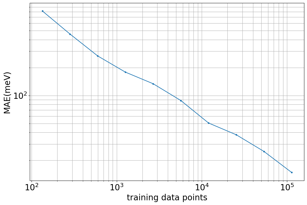
Figure 3: Learning curve for the QM9 dataset.

3.3 Demonstration of end-to-end differentiable simulations

The availability of automatic differentiation (AD) within a molecular dynamics package is beneficial beyond ML applications. Being able to compute gradients for all numerical operations opens up new avenues for sensitivity analysis, force field optimization and steered MD simulations, as well as simulations under highly complex constraints and restraints. To demonstrate these capabilities, the present example infers force field parameters from a short MD trajectory.

First, a small water box containing 97 water molecules and one Na⁺/Cl^- ion pair was simulated using the TIP3P water model with flexible bonds and angles. After energy minimization and NVT equilibration at 300 K, the simulation was run for 10 ps in the microcanonical ensemble. The simulation used a 1 fs time step, a 9 Å cutoff with 7.5 Å switch distance, and reaction field electrostatics. Coordinates and velocities were saved every 10 steps.

Next, all partial atomic charges $q$ in the system were annihilated (in practice, they were scaled by 0.01 to ensure non-vanishing gradients of the electrostatic potential). In order to infer $q$ from the MD trajectory, the integrator was initialized with snapshots $r(t_{i})$, $v(t_{i})$ from the trajectory. Then, 10 steps of simulation were run with the modified charges and the final positions from this short simulation were compared with the respective subsequent trajectory snapshot $r(t_{i+1})$. In other words, the simulation served as a parameterized propagator $Q:(r(t),v(t);q)\mapsto r(t+\delta_{t})$ with $\delta_{t}=10$ fs. Due to the AD capabilities within TorchMD, this propagator is end-to-end differentiable.

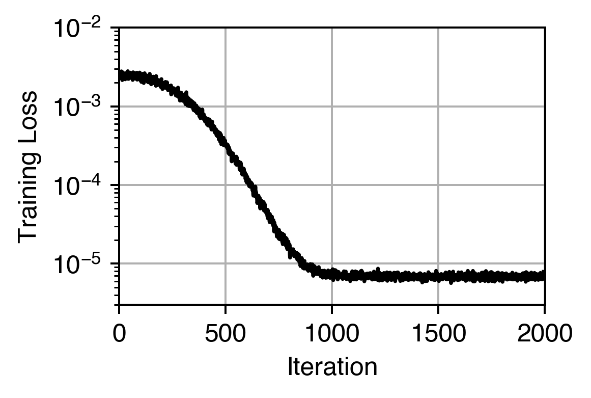
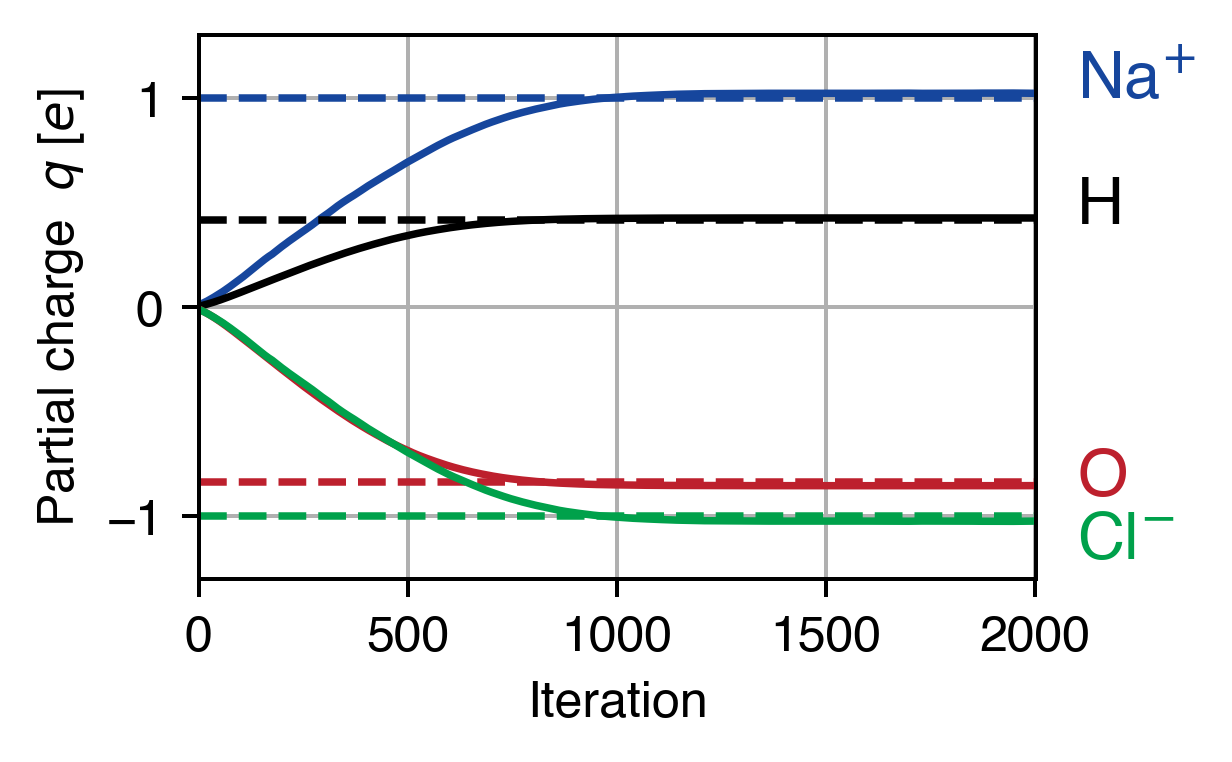
Figure 4: Inference of partial atomic charges $q$ from a short trajectory. Training loss (top) and charges (bottom) during training.

To recover the charges, we minimized the loss function

$$L\big{(}r(t_{i}),v(t_{i});q\big{)}=\|Q(r(t_{i}),v(t_{i});q)-r(t_{i+1})\|_{2}^{2},$$

i.e. the mean-squared distance between the ground-truth trajectory and the propagated coordinates (taking into account periodic boundary conditions). This loss function is differentiable with respect to the charges $q$ so that gradients can be obtained via backpropagation. Training was performed using Adam with a learning rate of $10^{-3}$ over one snapshot at a time. To enforce net neutrality, the positive charges ($q_{H}$ and $q_{\mathrm{Na}^{+}}$) were implicitly obtained from the oxygen and chlorine charges and only $q_{O}$ and $q_{\mathrm{Cl}^{-}}$ were explicitly optimized. Figure 4 shows the evolution of the training loss and the partial atomic charges during training. After just one epoch (1000 iterations), the original charges were recovered up to 3% accuracy.

3.4 Coarse-graining all-atom systems

For our last application example, we built two coarse-grained models of chignolin: one solely based on $\alpha$-carbon atoms (CA) and another one based on $\alpha$-carbon and $\beta$-carbon atoms (CACB) (Fig.5).

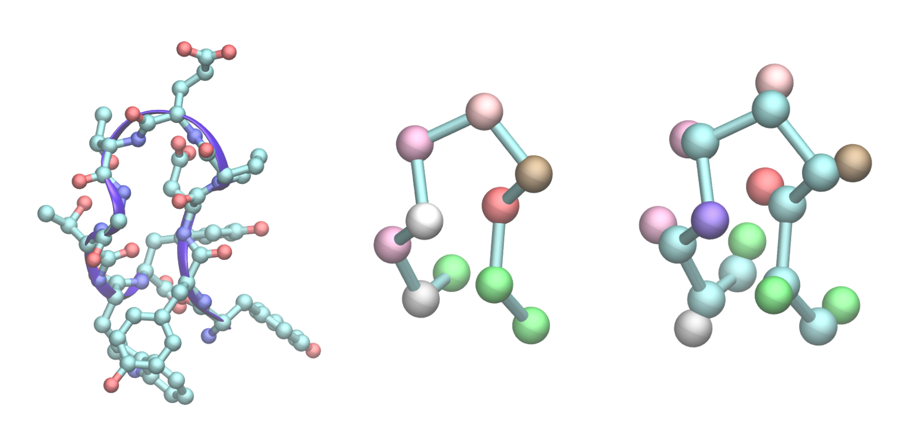
Figure 5: Miniprotein chignolin: heavy-atom representation (left) and coarse-grained representations: CA beads connected by bonds (middle), CA and CB beads connected by bonds (right). The beads in coarse grained representations were coloured by bead type.

3.4.1 Training data

We selected the CLN025 variant of chignolin (sequence YYDPETGTWY), which forms a $\beta$-hairpin turn while folded (Figure 5). Due to its small size (10 amino-acids) and fast folding, it has been extensively studied with MD ^{39, 40, 41, 42, 43, 44}. Training data was obtained from all-atom simulation of the protein in explicit solvent with ACEMD³⁰ on the GPUGRID.net distributed computing network.⁴⁵ The system containing one chignolin chain was solvated in a cubic box of 40 Å, containing 1881 water molecules and two Na⁺ ions. The system was simulated at 350 K with CHARMM22* force field ⁴⁶ and TIP3P model of water.⁴⁷ A Langevin integrator was used with a damping constant of $0.1\text{\,}{\mathrm{ps}}^{-1}$. Integration time step was set to 4 fs, with heavy hydrogen atoms (scaled up to four times the hydrogen mass) and holonomic constrains on all hydrogen-heavy atom bond terms ⁴⁸. Electrostatics were computed using Particle Mesh Ewald with a cutoff distance of 9 Å and a grid spacing of 1 Å. We used an adaptive sampling approach ⁴⁹ where new simulations were started from the least explored states. As a result we obtained a total simulation time of $180\text{\,}\mathrm{\SIUnitSymbolMicro s}$ with forces and coordinates saved every 100 ps giving a total of $1.8\times 10^{6}$ frames.

To obtain the training data for the CA model, the initial training set of coordinates and forces was filtered to retain only CA atoms positions and forces. In this example, a coarse grained system contains 10 beads, built out of seven unique types of beads, one for each amino acid type. The training set for CACB model was prepared in a similar fashion, filtering both CA and CB atoms, and achieving 19 beads and 8 unique types of beads, as all CA atoms were classified as one bead type with the exception of glycine and each CB was assigned an amino acid-specific bead type. Details of bead selection for both models are described in Supporting Methods.

3.4.2 Neural network potential training

For coarse-grained simulations it is important to provide some prior potentials in order to limit the space that the dynamics can visit to the space sampled in the training data⁹. All the terms of the force-field could be applied, but for simplicity we limit them to bonds and repulsions. Bonds prevent the protein polymer chain from breaking and repulsions stop computing NNP on very close atom distances where there is no data.

For pairwise bonded terms, we used the all-atom training data to construct distance histograms for each pair of bonded bead types. Specifically, for each bonded pair, we counted the fraction of time that the respective distance spent in an equally-spaced bin in a distance range appropriate to the bead selection, 3.55 Å and 4.2 Å for all bonds between $\alpha$ carbon beads, and 1.3 Å and 1.8 Å for all bonds between $\alpha$ carbon and $\beta$ carbon. The distance distributions were Boltzmann-inverted to obtain free-energy profiles, and these were used to fit the equilibrium distance $r_{0}$ and the spring constant $k$ of the respective harmonic potential

$$V^{\mathrm{(prior)}}_{\mathrm{harmonic}}(r)=k(r-r_{0})^{2}+V_{0},$$

where $r$ is the distance between the beads involved in the bond.

Priors for non-bonded repulsive terms were derived analogously. Distance histograms were constructed with 30 equally-spaced distance bins between 3 Å and 6 Å and were used to fit the parameter $\epsilon$ of the repulsive potential

$$V^{\mathrm{(prior)}}_{\mathrm{repulsive}}(r)=4\epsilon r^{-6}+V_{0},$$

where $r$, as above, is the distance between the non-bonded beads. In fitting the potential curves we corrected for the reference state by normalizing counts of each bin by the volume of the corresponding spherical shell. Non-linear curve fits were performed with the Levenberg-Marquardt method of the SciPy package ⁵⁰.

The parameters of the prior forces are stored in a YAML force field file. Plots presenting the quality of fits are included in the Supporting Information (Fig. S1-S4) as well as YAML files describing prior force field.

Based on resulting prior force field and input coordinates, we calculated a set of prior forces acting on the beads and then deducted them form true forces, resulting in a set of forces that we refer to as delta-forces. Along with coordinates, delta-forces were used as the input for training. In the case of CA model embeddings correspond to integers unique for each amino acid type. For CACB model all $\alpha$ carbons have the same embedding with the exception of glycine and each $\beta$ carbon has an embedding unique for each amino acid type.

The network was trained using force matching approach, where a predicted force is compared to a true force from the training set ^{9, 8}. In the example presented here, the network consisted of 3 interaction layers, 128 filters used in continuous-filter convolution, 128 features to describe atomic environments, 9 Å cutoff radius and 150 Gaussian functions for CA model and $300$ Gaussians for CACB model. Increasing the number of Gaussian functions for CACB model was found to provide a higher stability of the model and prevent forming collapsed non-physical structures during the simulation. Models for simulation were selected when the validation loss reached a plateau. The training and validation loss as well as learning rates are presented in Supporting Figure 5.

3.4.3 Simulation of the NNP

⬇

device: cuda:0

log_dir: sim_out_dir

output: output

topology: cln_ca_top.psf

coordinates: cln_ca_init_coords.xtc

replicas: 10

forcefield: cln_priors.yaml

forceterms:

- Bonds

- RepulsionCG

external:

module: torchmdnet.nnp.calculators.torchmdcalc

embeddings: [ 4, 4, 5, 8, 6, 13, 2, 13, 7, 4]

file: train/epoch=80.ckpt

langevin_gamma: 1

langevin_temperature: 350

temperature: 350

precision: double

seed: 1

output_period: 1000

save_period: 1000

steps: 10000000

timestep: 1

Figure 6: An example of a simulation input file

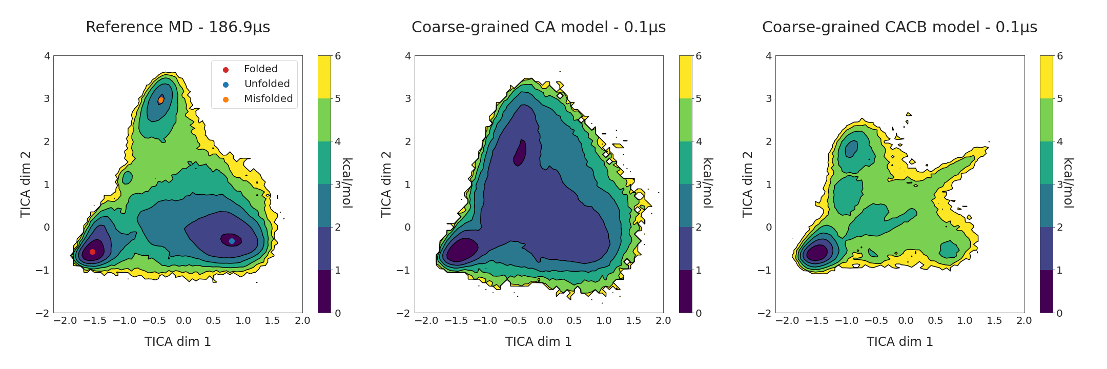
Figure 7: Two-dimensional free energy surfaces for the reference all-atom MD simulations (left) and the two coarse-grained models, CA (center) and CACB (right). The free energy surface for each simulation set was obtained by binning over the first two TICA dimensions, dividing them into a 120 $\times$ 120 grid, and averaging the weights of the equilibrium probability in each bin computed by the Markov state model. The reference MD simulations plot displays the locations of the three energy minima on the surface, corresponding to folded state (red dot), unfolded conformations (blue dot) and a misfolded state (orange dot). Both reference MD and coarse-grained simulations were performed at 350K.

The combinations of the force fields covering prior forces and the trained networks are used to simulate both CA and CACB systems with TorchMD. We introduce the parameters of the simulation as a YAML-formatted configuration file (Figure 6), although the simulation can be also started from command line. The network is introduced to TorchMD as an external force, with specified network’s location, embeddings and a calculator. An external force calculator class must have a "calculate" method that returns a tuple with energy and forces tensors. In our case, for both models, we run the simulation at 350K for 10 ns with 1 fs timestep, saving the output every 1000 fs. Note that while the simulations use a small timestep, the effective dynamics of the coarse-grained systems is much faster than the all-atom MD system as the coarse-grained model is supposed to reproduce the energetics but with much faster kinetics. Since TorchMD can easily handle parallel dynamics, we concurrently run ten simulations, of which five start from the folded state and five from unfolded conformations.

The free energy surfaces obtained with a time-lagged independent component analysis (TICA)⁵¹ for the all-atom baseline simulations and the coarse-grained simulations obtained with TorchMD are presented in Figure 7. The energy landscapes are obtained from binning the configurations over the first two TICA dimensions and computing the average of the equilibrium probability on each bin, obtained by Markov state model analysis of the microstate of each configuration. To support TICA plots, we included plots with RMSD values for the first 2 ns of representative trajectories for both models with different starting points (Fig. 8). Plots presenting full trajectories are included in Supporting Information (Fig.S6-S9). Neither SchNet nor prior energy terms can enforce chirality in the system, because they both work purely on the distances between the beads. Therefore, the RMSD plots were supplemented with RMSD values of the trajectory’s mirror image.

Results show that the coarse-grained simulations for both models were able to obtain several folding and unfolding events for chignolin. The energy landscapes for the CA model show that it captured the folded state as a global minimum of energy. The simulations also covers other minima representing unfolded and misfolded states. However, they do not recreate the energy barriers connecting these basins (as expected), which is better seen on the one-dimensional free energy surfaces (Fig.S10). The CACB model also detects the global minimum correctly, but fails at guessing the free energy of the unfolded region. Overall the simulation is less stable than for CA model and the misfolded state minimum is incorrectly located.

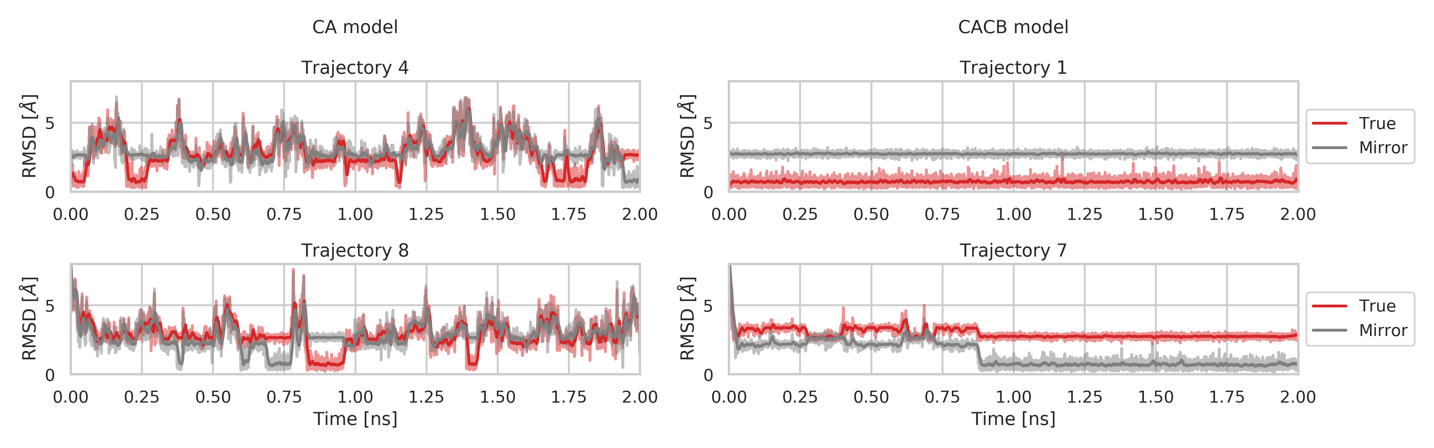
Figure 8: The RMSD values across the first 2 ns of the unmodified trajectory (True, red) and a mirror image of the original trajectory (Mirror, gray) for CA model (on the left) and CACB model (on the right). Trajectory 4 (top left panel) and Trajectory 1 (top right panel) are examples of a trajectories started from the folded state for CA model and CACB model, respectively. Trajectory 8 (bottom left panel) and Trajectory 7 (bottom right panel) are examples of trajectories started from elongated chain for CA model and CACB model, respectively. A moving average of 100 frames is represented as darker lines. The full 10 ns of each simulation is included in Supporting Figures S6-S9.

4 Conclusion

In this paper we demonstrated TorchMD, a PyTorch-based molecular dynamics engine for biomolecular simulations with machine learning capabilities. We have shown several possible applications ranging from Amber all-atom simulations, to end-to-end learning of parameters and finally a coarse-grained neural network potential for protein folding. In particular, building a NNP for protein folding requires supplementing it with asymptotic, analytical potentials for bonds and repulsions to prevent exploring conformations not visited in the training data in which the predictions of NNP are unreliable. We have shown how to coarse-grain a protein into either $\alpha$-carbon atoms or $\alpha$-carbon and $\beta$-carbon atoms. Currently, CA model seems to work the best but future research will indicate which models are better suited for a more diverse set of targets. TorchMD end-to-end differentiability of its parameters is a feature that projects such as the Open Force Field Initiative ⁵² can potentially exploit. Furthermore, for additional speed we plan to facilitate the integration of machine learning potentials in OpenMM⁵³ and ACEMD ³⁰. Meanwhile, we believe that TorchMD can play an important role by facilitating experimentation between ML and MD fields, speeding up the model-train-evaluate prototyping cycle, and promoting the adoption of data-based approaches in molecular simulations. All the code machinery to produce the models is made available for practitioners at github.com/torchmd.

. SD thanks the Chan Zuckerberg initiative for funding. We thank the volunteers of GPUGRID.net for donating computing time. This project has received funding from the European Union’s Horizon 2020 research and innovation programme under grant agreement No 823712.

References

- Lee et al. 2009 Lee, E. H.; Hsin, J.; Sotomayor, M.; Comellas, G.; Schulten, K. Discovery Through the Computational Microscope. Structure 2009, 17, 1295–1306
- Ponder and Case 2003 Ponder, J. W.; Case, D. A. Advances in Protein Chemistry; Protein Simulations; Academic Press, 2003; Vol. 66; pp 27–85
- Martínez-Rosell et al. 2017 Martínez-Rosell, G.; Giorgino, T.; Harvey, M. J.; de Fabritiis, G. Drug Discovery and Molecular Dynamics: Methods, Applications and Perspective Beyond the Second Timescale. Current Topics in Medicinal Chemistry 2017, 17, 2617–2625
- Schütt et al. 2017 Schütt, K.; Kindermans, P.-J.; Felix, H. E. S.; Chmiela, S.; Tkatchenko, A.; Müller, K.-R. Schnet: A continuous-filter convolutional neural network for modeling quantum interactions. Advances in neural information processing systems. 2017; pp 991–1001
- Schütt et al. 2018 Schütt, K. T.; Sauceda, H. E.; Kindermans, P.-J.; Tkatchenko, A.; Müller, K.-R. SchNet–A deep learning architecture for molecules and materials. The Journal of Chemical Physics 2018, 148, 241722
- Ruza et al. 2020 Ruza, J.; Wang, W.; Schwalbe-Koda, D.; Axelrod, S.; Harris, W. H.; Gómez-Bombarelli, R. Temperature-transferable coarse-graining of ionic liquids with dual graph convolutional neural networks. The Journal of Chemical Physics 2020, 153, 164501
- Duvenaud et al. 2015 Duvenaud, D. K.; Maclaurin, D.; Iparraguirre, J.; Bombarell, R.; Hirzel, T.; Aspuru-Guzik, A.; Adams, R. P. Convolutional networks on graphs for learning molecular fingerprints. Advances in neural information processing systems. 2015; pp 2224–2232
- Husic et al. 2020 Husic, B. E.; Charron, N. E.; Lemm, D.; Wang, J.; Pérez, A.; Majewski, M.; Krämer, A.; Chen, Y.; Olsson, S.; de Fabritiis, G.; Noé, F., et al. Coarse Graining Molecular Dynamics with Graph Neural Networks. J. Chem. Phys. 2020, 153, 194101
- Wang et al. 2019 Wang, J.; Olsson, S.; Wehmeyer, C.; Pérez, A.; Charron, N. E.; De Fabritiis, G.; Noé, F.; Clementi, C. Machine learning of coarse-grained molecular dynamics force fields. ACS central science 2019, 5, 755–767
- Nüske et al. 2019 Nüske, F.; Boninsegna, L.; Clementi, C. Coarse-graining molecular systems by spectral matching. The Journal of chemical physics 2019, 151, 044116
- Wang et al. 2020 Wang, J.; Chmiela, S.; Müller, K.-R.; Noé, F.; Clementi, C. Ensemble learning of coarse-grained molecular dynamics force fields with a kernel approach. The Journal of Chemical Physics 2020, 152, 194106
- Zhang et al. 2018 Zhang, L.; Han, J.; Wang, H.; Car, R.; E, W. DeePCG: constructing coarse-grained models via deep neural networks. arXiv:1802.08549 2018,
- Wang and Gómez-Bombarelli 2019 Wang, W.; Gómez-Bombarelli, R. Coarse-graining auto-encoders for molecular dynamics. npj Computational Materials 2019, 5, 1–9
- Wang et al. 2020 Wang, W.; Yang, T.; Harris, W. H.; Gómez-Bombarelli, R. Active learning and neural network potentials accelerate molecular screening of ether-based solvate ionic liquids. Chem. Commun. 2020, 56, 8920–8923
- Marrink and Tieleman 2013 Marrink, S. J.; Tieleman, D. P. Perspective on the Martini model. Chemical Society Reviews 2013, 42, 6801–6822
- Machado et al. 2019 Machado, M. R.; Barrera, E. E.; Klein, F.; Sóñora, M.; Silva, S.; Pantano, S. The SIRAH 2.0 Force Field: Altius, Fortius, Citius. Journal of Chemical Theory and Computation 2019, 15, 2719–2733
- Saunders and Voth 2013 Saunders, M. G.; Voth, G. A. Coarse-Graining Methods for Computational Biology. Annu. Rev. Biophys. 2013, 42, 73–93
- Izvekov and Voth 2005 Izvekov, S.; Voth, G. A. A Multiscale Coarse-Graining Method for Biomolecular Systems. J. Phys. Chem. B 2005, 109, 2469–2473
- Noid 2013 Noid, W. G. Perspective: Coarse-grained models for biomolecular systems. J. Chem. Phys. 2013, 139, 090901
- Clementi 2008 Clementi, C. Coarse-grained models of protein folding: Toy-models or predictive tools? Curr. Opin. Struct. Biol. 2008, 18, 10–15
- Paszke et al. 2019 Paszke, A.; Gross, S.; Massa, F.; Lerer, A.; Bradbury, J.; Chanan, G.; Killeen, T.; Lin, Z.; Gimelshein, N.; Antiga, L.; Desmaison, A.; Kopf, A.; Yang, E.; DeVito, Z.; Raison, M.; Tejani, A.; Chilamkurthy, S.; Steiner, B.; Fang, L.; Bai, J.; Chintala, S. In Advances in Neural Information Processing Systems 32; Wallach, H., Larochelle, H., Beygelzimer, A., d'Alché-Buc, F., Fox, E., Garnett, R., Eds.; Curran Associates, Inc., 2019; pp 8024–8035
- Gao et al. 2020 Gao, X.; Ramezanghorbani, F.; Isayev, O.; Smith, J.; Roitberg, A. TorchANI: A Free and Open Source PyTorch Based Deep Learning Implementation of the ANI Neural Network Potentials. 2020, Publisher: ChemRxiv
- Wang et al. 2020 Wang, Y.; Fass, J.; Chodera, J. D. End-to-End Differentiable Molecular Mechanics Force Field Construction. 2020; preprint arXiv:2010.01196
- Bradbury et al. 2018 Bradbury, J.; Frostig, R.; Hawkins, P.; Johnson, M. J.; Leary, C.; Maclaurin, D.; Wanderman-Milne, S. JAX: composable transformations of Python+NumPy programs. 2018; http://github.com/google/jax
- Schoenholz and Cubuk 2019 Schoenholz, S. S.; Cubuk, E. D. JAX, M.D.: End-to-End Differentiable, Hardware Accelerated, Molecular Dynamics in Pure Python. 2019; preprint arXiv:1912.04232
- Zhao 2020 Zhao, Y. Time Machine. GitHub. Note: https://github.com/proteneer/timemachine 2020,
- Yao et al. 2018 Yao, K.; Herr, J. E.; Toth, D. W.; Mckintyre, R.; Parkhill, J. The TensorMol-0.1 model chemistry: a neural network augmented with long-range physics. Chemical Science 2018, 9, 2261–2269, Publisher: The Royal Society of Chemistry
- Schütt et al. 2019 Schütt, K. T.; Kessel, P.; Gastegger, M.; Nicoli, K. A.; Tkatchenko, A.; Müller, K.-R. SchNetPack: A Deep Learning Toolbox For Atomistic Systems. Journal of Chemical Theory and Computation 2019, 15, 448–455
- Tironi et al. 1995 Tironi, I. G.; Sperb, R.; Smith, P. E.; van Gunsteren, W. F. A generalized reaction field method for molecular dynamics simulations. The Journal of Chemical Physics 1995, 102, 5451–5459
- Harvey et al. 2009 Harvey, M. J.; Giupponi, G.; Fabritiis, G. D. ACEMD: accelerating biomolecular dynamics in the microsecond time scale. Journal of chemical theory and computation 2009, 5, 1632–1639
- Shirts et al. 2017 Shirts, M. R.; Klein, C.; Swails, J. M.; Yin, J.; Gilson, M. K.; Mobley, D. L.; Case, D. A.; Zhong, E. D. Lessons learned from comparing molecular dynamics engines on the SAMPL5 dataset. Journal of Computer-Aided Molecular Design 2017, 31, 147–161
- Maier et al. 2015 Maier, J. A.; Martinez, C.; Kasavajhala, K.; Wickstrom, L.; Hauser, K. E.; Simmerling, C. ff14SB: Improving the Accuracy of Protein Side Chain and Backbone Parameters from ff99SB. Journal of Chemical Theory and Computation 2015, 11, 3696–3713
- Christensen et al. 2020 Christensen, A. S.; Bratholm, L. A.; Faber, F. A.; Anatole von Lilienfeld, O. FCHL revisited: Faster and more accurate quantum machine learning. The Journal of Chemical Physics 2020, 152, 044107
- Falcon 2019 Falcon, W. PyTorch Lightning. GitHub. Note: https://github.com/PyTorchLightning/pytorch-lightning 2019,
- Ramakrishnan et al. 2014 Ramakrishnan, R.; Dral, P. O.; Rupp, M.; von Lilienfeld, O. A. Quantum chemistry structures and properties of 134 kilo molecules. Scientific Data 2014, 1
- Honda et al. 2008 Honda, S.; Akiba, T.; Kato, Y. S.; Sawada, Y.; Sekijima, M.; Ishimura, M.; Ooishi, A.; Watanabe, H.; Odahara, T.; Harata, K. Crystal structure of a ten-amino acid protein. Journal of the American Chemical Society 2008, 130, 15327–15331
- Kingma and Ba 2014 Kingma, D. P.; Ba, J. Adam: A method for stochastic optimization. arXiv preprint arXiv:1412.6980 2014,
- Vapnik 2013 Vapnik, V. The nature of statistical learning theory; Springer science & business media, 2013
- Lindorff-Larsen et al. 2011 Lindorff-Larsen, K.; Piana, S.; Dror, R. O.; Shaw, D. E. How fast-folding proteins fold. Science 2011, 334, 517–520
- Beauchamp et al. 2012 Beauchamp, K. A.; McGibbon, R.; Lin, Y.-S.; Pande, V. S. Simple few-state models reveal hidden complexity in protein folding. Proceedings of the National Academy of Sciences 2012, 109, 17807–17813
- Husic et al. 2016 Husic, B. E.; McGibbon, R. T.; Sultan, M. M.; Pande, V. S. Optimized parameter selection reveals trends in Markov state models for protein folding. The Journal of chemical physics 2016, 145, 194103
- McKiernan et al. 2017 McKiernan, K. A.; Husic, B. E.; Pande, V. S. Modeling the mechanism of CLN025 beta-hairpin formation. The Journal of chemical physics 2017, 147, 104107
- Sultan and Pande 2018 Sultan, M. M.; Pande, V. S. Automated design of collective variables using supervised machine learning. The Journal of chemical physics 2018, 149, 094106
- Scherer et al. 2019 Scherer, M. K.; Husic, B. E.; Hoffmann, M.; Paul, F.; Wu, H.; Noé, F. Variational selection of features for molecular kinetics. The Journal of chemical physics 2019, 150, 194108
- Buch et al. 2010 Buch, I.; Harvey, M. J.; Giorgino, T.; Anderson, D. P.; De Fabritiis, G. High-throughput all-atom molecular dynamics simulations using distributed computing. Journal of chemical information and modeling 2010, 50, 397–403
- Piana et al. 2011 Piana, S.; Lindorff-Larsen, K.; Shaw, D. E. How robust are protein folding simulations with respect to force field parameterization? Biophysical Journal 2011, 100
- Jorgensen et al. 1983 Jorgensen, W. L.; Chandrasekhar, J.; Madura, J. D.; Impey, R. W.; Klein, M. L. Comparison of simple potential functions for simulating liquid water. J. Chem. Phys. 1983, 79, 926–935
- Feenstra et al. 1999 Feenstra, K. A.; Hess, B.; Berendsen, H. J. Improving efficiency of large time-scale molecular dynamics simulations of hydrogen-rich systems. J. Comput. Chem. 1999, 20, 786–798
- Doerr and De Fabritiis 2014 Doerr, S.; De Fabritiis, G. On-the-Fly Learning and Sampling of Ligand Binding by High- Throughput Molecular Simulations. Journal of Chemical Theory and Computation 2014,
- Virtanen et al. 2020 Virtanen, P.; Gommers, R.; Oliphant, T. E.; Haberland, M.; Reddy, T.; Cournapeau, D.; Burovski, E.; Peterson, P.; Weckesser, W.; Bright, J.; van der Walt, S. J.; Brett, M.; Wilson, J.; Millman, K. J.; Mayorov, N.; Nelson, A. R. J.; Jones, E.; Kern, R.; Larson, E.; Carey, C. J.; Polat, I.; Feng, Y.; Moore, E. W.; VanderPlas, J.; Laxalde, D.; Perktold, J.; Cimrman, R.; Henriksen, I.; Quintero, E. A.; Harris, C. R.; Archibald, A. M.; Ribeiro, A. H.; Pedregosa, F.; van Mulbregt, P. SciPy 1.0: fundamental algorithms for scientific computing in Python. Nature Methods 2020, 17, 261–272
- Pérez-Hernández et al. 2013 Pérez-Hernández, G.; Paul, F.; Giorgino, T.; De Fabritiis, G.; Noé, F. Identification of slow molecular order parameters for Markov model construction. The Journal of chemical physics 2013, 139, 07B604_1
- Mobley et al. 2018 Mobley, D. L.; Bannan, C. C.; Rizzi, A.; Bayly, C. I.; Chodera, J. D.; Lim, V. T.; Lim, N. M.; Beauchamp, K. A.; Shirts, M. R.; Gilson, M. K.; Eastman, P. K. Open Force Field Consortium: Escaping atom types using direct chemical perception with SMIRNOFF v0.1. 2018; Biorxiv preprint 10.1101/286542
- Eastman et al. 2017 Eastman, P.; Swails, J.; Chodera, J. D.; McGibbon, R. T.; Zhao, Y.; Beauchamp, K. A.; Wang, L.-P.; Simmonett, A. C.; Harrigan, M. P.; Stern, C. D.; Wiewiora, R. P.; Brooks, B. R.; Pande, V. S. OpenMM 7: Rapid development of high performance algorithms for molecular dynamics. PLOS Computational Biology 2017, 13, e1005659