Warped Gaussian Processes in Remote Sensing Parameter Estimation and Causal Inference

Abstract

This paper introduces warped Gaussian processes (WGP) regression in remote sensing applications. WGP models output observations as a parametric nonlinear transformation of a GP. The parameters of such prior model are then learned via standard maximum likelihood. We show the good performance of the proposed model for the estimation of oceanic chlorophyll content from multispectral data, vegetation parameters (chlorophyll, leaf area index, and fractional vegetation cover) from hyperspectral data, and in the detection of the causal direction in a collection of 28 bivariate geoscience and remote sensing causal problems. The model consistently performs better than the standard GP and the more advanced heteroscedastic GP model, both in terms of accuracy and more sensible confidence intervals.

I Introduction

With the forthcoming superspectral satellite missions dedicated to land, vegetation and ocean monitoring, an unprecedented data stream is now available and will increase in following years. Automatic efficient techniques for spatial and temporal explicit quantification of Earth properties are an urgent need. When it comes to the implementation of candidate retrieval methods into operational data processing chains, like e.g. the Copernicus’ Sentinels, it is mandatory to invest in models that are both accurate and robust, but also requiring minimum user intervention for fitting parameters, and that provide sensible confidence intervals for the predictions. This is the scenario where this paper is placed.

In this paper, we focus on the Bayesian non-parametric framework in general, and in Gaussian processes (GPs) [1], which have yielded very good performance in the last years in many geoscience and remote sensing problems, such as biophysical parameter estimation, radiative transfer model emulation and causal inference from empirical data [2, 3]. Despite the very good performance of standard GPs, inclusion of prior knowledge respecting signal characteristics is mandatory to achieve state-of-the-art results, and in turn make parameter tuning simpler and less sensitive to initializations. This can be achieved by designing kernel functions that respect signal smoothness in space or time [4, 5], combining multi-scale and multi-resolution of the features [6, 5], or by designing regularizers to encompass signal and noise relations [7].

Little attention has been paid, however, to the statistical characteristics of the output, observed variable. Actually, we should note an important observation: GP modeling assumes that the target data is distributed as a multivariate Gaussian and that observations are buried in constant power (homoscedastic) Gaussian noise as well. These assumptions allow model tractability, yet sometimes they are unrealistic in practice. Commonly one performs ad hoc pre-processing of the data to achieve transformations of the observed variable to make it look as a Gaussian. It is customary to apply logarithmic, exponential, power or logistic transformations to spectral ratios. This is not only arbitrary, but somehow contradictory since first data is transformed by a parametric function, and then, a non-parametric GP model is fitted. In this paper, we propose a GP that automatically learns the optimal transformation to be applied. The method is called warped GP (WGP) [8] and commonly leads to more accurate results over standard and more advanced GPs. It also leads to more sensible confidence intervals and gives important insights on the non-linearity of the problem. The WGP model actually generalizes standard GPs, and allows to deal with non-Gaussian processes and non-Gaussian noise.

The remainder of the paper is organized as follows. Section 2 reviews the warped GP regression method. Section 3 details the data characteristics used in this paper. Section 4 gives the experimental results for several problems: (i) the estimation of chlorophyll-a concentration from remote sensing upwelling radiance just above the ocean surface, estimation of biophysical parameters (chlorophyll-a, leaf area index, and fractional vegetation cover) from hyperspectral data, and the problem of cause-effect discovery from pairs of observational data. Finally, Section 5 concludes the paper and outlines the further work.

II Warped Gaussian Processes

This section reviews the theory of GP regression, introduces the warped GP model, and describes the parameterization of both the covariance and the warping functions.

II-A Gaussian Process Regression (GP)

Standard regression approximates observations (often referred to as outputs) $\{y_{i}\}_{i=1}^{N}$ as the sum of some unknown latent function $f({\mathbf{x}})$ of the inputs $\{{\mathbf{x}}_{i}\in\mathbb{R}^{D}\}_{i=1}^{N}$ plus constant power Gaussian noise, that is:

$$y_{i}=f({\mathbf{x}}_{i})+\varepsilon_{i},~{}~{}~{}~{}\varepsilon_{i}\sim\mathcal{N}(0,\sigma_{n}^{2}).$$ (1)

Instead of proposing a parametric form for $f({\mathbf{x}})$ and learning its parameters in order to fit observed data well, GP regression proceeds in a Bayesian, non-parametric way. A zero mean GP prior is placed on the latent function $f({\boldsymbol{\mathbf{x}}})$ and a Gaussian prior is used for each latent noise term $\varepsilon_{i}$, $f({\boldsymbol{\mathbf{x}}})\;\sim\;\mathcal{GP}({\boldsymbol{\mathbf{0}}},k_{\boldsymbol{\mathbf{\theta}}}({\boldsymbol{\mathbf{x}}},{\boldsymbol{\mathbf{x}}}^{\prime}))$, where $k_{\boldsymbol{\mathbf{\theta}}}({\boldsymbol{\mathbf{x}}},{\boldsymbol{\mathbf{x}}}^{\prime})$ is a covariance function parameterized by a vector ${\boldsymbol{\mathbf{\theta}}}$, and $\sigma_{n}^{2}$ is a parameter accounting for the noise power. Essentially, a Gaussian process is a stochastic process whose marginals are distributed as a multivariate Gaussian. In particular, given the priors $\mathcal{GP}$, samples drawn from $f({\mathbf{x}})$ at the set of locations $\{{\mathbf{x}}_{i}\}_{i=1}^{N}$ follow a joint multivariate Gaussian with zero mean and covariance matrix ${\boldsymbol{\mathbf{K_{\boldsymbol{\mathbf{ff}}}}}}$ with $[{\boldsymbol{\mathbf{K_{\boldsymbol{\mathbf{ff}}}}}}]_{ij}=k_{\boldsymbol{\mathbf{\theta}}}({\boldsymbol{\mathbf{x}}}_{i},{\boldsymbol{\mathbf{x}}}_{j})$.

If we consider a test location ${\mathbf{x}}_{*}$ with corresponding output $y_{*}$, the $\mathcal{GP}$ defines a joint prior distribution between the observations ${{\boldsymbol{\mathbf{y}}}}\equiv\{y_{i}\}_{i=1}^{N}$ and $y_{*}$. Collecting available data in ${\cal D}\equiv\{({\boldsymbol{\mathbf{x}}}_{i},y_{i})|i=1,\ldots N\}$, it is possible to analytically compute the posterior distribution over the unknown output $y_{*}$:

$$\begin{split}p(y_{*}|{\boldsymbol{\mathbf{x}}}_{*},{\cal D})&=\mathcal{N}(y_{*}|\mu_{\text{GP}*},\sigma_{\text{GP}*}^{2})\\ \mu_{\text{GP}*}&={\boldsymbol{\mathbf{k}}}_{{\boldsymbol{\mathbf{f}}}*}^{\top}({\boldsymbol{\mathbf{K}}}_{{\boldsymbol{\mathbf{ff}}}}+\sigma_{n}^{2}{\boldsymbol{\mathbf{I}}})^{-1}{\boldsymbol{\mathbf{y}}}={\boldsymbol{\mathbf{k}}}_{{\boldsymbol{\mathbf{f}}}*}^{\top}\boldsymbol{\alpha}\\ \sigma_{\text{GP}*}^{2}&=\sigma_{n}^{2}+k_{**}-{\boldsymbol{\mathbf{k}}}_{{\boldsymbol{\mathbf{f}}}*}^{\top}({\boldsymbol{\mathbf{K}}}_{{\boldsymbol{\mathbf{ff}}}}+\sigma_{n}^{2}{\boldsymbol{\mathbf{I}}})^{-1}{\boldsymbol{\mathbf{k}}}_{{\boldsymbol{\mathbf{f}}}*}.\end{split}$$ (2)

The corresponding parameters $\{{\boldsymbol{\mathbf{\theta}}},\sigma_{n}\}$ are typically selected by Type-II Maximum Likelihood, using the marginal likelihood (also called evidence) of the observations, which is also analytic (explicitly conditioning on ${\boldsymbol{\mathbf{\theta}}}$ and $\sigma_{n}$):

$$\log p({\boldsymbol{\mathbf{y}}}|{\boldsymbol{\mathbf{\theta}}},\sigma_{n})=\log\mathcal{N}({{\boldsymbol{\mathbf{y}}}}|{\boldsymbol{\mathbf{0}}},{{\boldsymbol{\mathbf{K}}}}_{\boldsymbol{\mathbf{ff}}}+\sigma_{n}^{2}{\boldsymbol{\mathbf{I}}}).$$ (3)

II-B Warped Gaussian Process Regression (GP)

In real applications, the distribution of the observations is very often not Gaussian, due to the sampling strategies followed during the protocols in data collection or because of the natural variability of the problem. Very often, in practice, one remedies that by transforming the observed variable to make it look like a Gaussian. Actually, it is a standard practice to apply logarithmic or exponential functions to this end.

In this paper, we use a GP model that automatically learns the optimal transformation by warping the predictions of a standard GP model. The method is called warped GP [8], and essentially warps observations ${\bf y}$ through a nonlinear parametric function $g$ to a latent space:

$$z_{i}=g(y_{i},\psi)=g(f({\bf x}_{i})+\varepsilon_{i}),$$

where $g$ is a function with scalar inputs parameterized by ${\boldsymbol{\mathbf{\psi}}}$. Note that the new error term cannot be readily accessed or quantified, since g is a nonparametric function and does not factorize. The function $g$ must be monotonic, otherwise the probability measure will not be conserved in the transformation, and the distribution over the targets might not be valid [8]. It can be shown that replacing $y_{i}$ by $z_{i}$ into the standard GP model leads to an extended problem that can be solved by taking derivatives of the negative log likelihood function in (3), but now with respect to both ${\boldsymbol{\mathbf{\theta}}}$ and ${\boldsymbol{\mathbf{\psi}}}$ parameter vectors.

II-C Model parametrization

Owing to the probabilistic treatment, all GP variants yield a full posterior predictive distribution over $y_{*}$, it is possible to obtain not only mean predictions for test data, but also its uncertainty. The whole procedure only depends on a very small set of parameters; collectively grouped in ${\boldsymbol{\mathbf{\theta}}}$ for GP and in ${\boldsymbol{\mathbf{\psi}}}$ for WGP. Inference of the parameters and the weights $\boldsymbol{\alpha}$ can be performed using continuous optimization of the evidence in 3.

For both the GP and WGP models we need to define the covariance (kernel, or Gram) function $k(\cdot,\cdot)$, which should capture the similarity between samples. We used the standard Automatic Relevance Determination (ARD) covariance $k({\boldsymbol{\mathbf{x}}}_{i},{\boldsymbol{\mathbf{x}}}_{j})=\nu\exp(-\sum_{d=1}^{D}({x}_{i}^{d}-{x}_{j}^{d})^{2}/(2\sigma_{d}^{2}))$, which has given good performance in many problems [1, 3], where ${\boldsymbol{\mathbf{x}}}_{i}$ and ${\boldsymbol{\mathbf{x}}}_{j}$ are vectors. For GP, model parameters are collectively grouped in ${\boldsymbol{\mathbf{\theta}}}=\{\nu,\sigma_{n},\sigma_{1},\ldots,\sigma_{d}\}$. For the WGP we need to define a parametric smooth and monotonic form for $g$. In this paper we used:

$$g(y_{i};{\boldsymbol{\mathbf{\psi}}})=\sum_{\ell=1}^{L}a_{\ell}~{}\text{tanh}(b_{\ell}~{}y_{i}+c_{\ell}),~{}~{}~{}~{}a_{\ell},~{}b_{\ell}\geq 0,$$

where ${\boldsymbol{\mathbf{\psi}}}=\{{\bf a},{\bf b},{\bf c}\}$. Even though any other sensible parametrization could be used, this one is quite convenient since it yields a set of smooth steps whose size, steepness and position are controlled by $a_{\ell}$, $b_{\ell}$ and $c_{\ell}$ parameters, respectively. In the present work, we fixed $L=5$ after several experiments, while the latter parameters were inferred via standard maximum log-likelihood maximization.

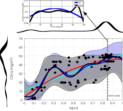
Figure 1: Scatterplot of NDVI vs LAI with predictive means (lines) and deviations (shaded areas) as well as the marginal distributions. The conditional densities at NDVI=0.85 (top of the figure) shows how the standard GP confidence intervals are symmetric while the WGP better captures the conditional distribution of the sample and yields asymmetric confidence intervals tighter around the more densely populated Chl-a regions.

II-D Illustration of a warped GP model

We illustrate the main difference between GPs and WGPs in the problem of estimating chlorophyll concentration (Chl-a) from the NDVI using in situ measurements (data description and experiments further explained in section III-B). Figure 1 shows the data distribution, as well as linear (cyan), second order polynomial (red), GP (blue), and WGP (black) fitting. In gray and blue shaded areas we provide the confidence intervals (mean$\pm$2 standard deviations) for the GP and WGP models, respectively. The marginals indicate a denser sampling of Chl-a in the NDVI region between [0.7,0.9], and reveal a non-Gaussian distribution of the Chl-a target variable. The main difference between standard GP and WGP arises on the shape of its confidence intervals, which is better observed in the conditional pdf, i.e. $p(y|\text{NVDI}=0.85)$. In top of Fig. 1, the standard GP yields a symmetric area around its mean, but the shape of the predictive distribution of WGP is more flexible and adapts better to the data distribution. Note that the conditional confidence interval in this case shows three different peaks, revealing higher confidence around the chlorophyll regions more densely sampled.

III Experimental results

We show the potential of WGP in the following three experiments: 1) estimation of ocean chlorophyll concentration from multispectral data; 2) vegetation parameter retrieval from hyperspectral images; and 3) causal inference in a set of 28 geosciences problems.

III-A Experiment 1: Ocean chlorophyll estimation

We focus here on the estimation of chlorophyll-a concentrations from remote sensing upwelling radiance just above the ocean surface. A variety of bio-optical algorithms have been developed to relate measurements of ocean radiance to in situ concentrations of phytoplankton pigments, and ultimately most of these algorithms demonstrate the potential of quantifying chlorophyll-a concentrations accurately from multispectral satellite ocean color data. In addition, we should note that most of the bio-optical models (such as Morel, CalCOFI and OC2/OC4 models) often rely on empirically adjusted nonlinear transformation of the observed variable (which is traditionally a ratio between bands). In this context, more robust and stable non-linear regression methods are desirable.

We used the SeaBAM dataset [9], which gathers 919 in situ pigment measurements around the United States and Europe. The dataset contains coincident in situ chlorophyll concentration and remote sensing reflectance measurements (Rrs($\lambda$), [sr^-1]) at some wavelengths (412, 443, 490, 510 and 555 nm) that are present in the SeaWiFS ocean color satellite sensor. The chlorophyll concentration values range varies from 0.019 to 32.79 mg/m³, revealing a clear exponential distribution. More information about the data can be obtained from http://seabass.gsfc.nasa.gov/seabam/seabam.html.

TABLE I: Bias (ME), accuracy (RMSE, MAE) and fitness (coefficient of correlation R) for different rates of training samples using both raw and empirically-transformed variable for the SeaBAM dataset.

	Raw				Empirical
	ME	RMSE	MAE	R	ME	RMSE	MAE	R
rate = 20%
GP	0.146 $\pm$ 0.142	1.836 $\pm$0.541	0.490 $\pm$0.175	0.765 $\pm$0.139	0.148 $\pm$ 0.112	2.390 $\pm$1.001	0.411 $\pm$0.098	0.736 $\pm$0.132
VHGP	0.252 $\pm$ 0.129	2.195 $\pm$0.342	0.530 $\pm$0.147	0.657 $\pm$0.119	0.141 $\pm$ 0.105	2.384 $\pm$1.017	0.410 $\pm$0.096	0.737 $\pm$0.134
WGP	0.143 $\pm$ 0.110	1.710 $\pm$0.337	0.401 $\pm$0.055	0.804 $\pm$0.071	0.146 $\pm$ 0.118	2.583 $\pm$1.122	0.445 $\pm$0.116	0.686 $\pm$0.149
rate = 50%
GP	0.133 $\pm$ 0.110	2.036 $\pm$0.468	0.453 $\pm$0.057	0.765 $\pm$0.106	0.149 $\pm$ 0.144	2.024 $\pm$1.689	0.349 $\pm$0.142	0.823 $\pm$0.130
VHGP	0.183 $\pm$ 0.119	1.786 $\pm$0.454	0.398 $\pm$0.046	0.789 $\pm$0.090	0.146 $\pm$ 0.116	1.934 $\pm$1.272	0.343 $\pm$0.115	0.828 $\pm$0.117
WGP	0.069 $\pm$ 0.050	1.318 $\pm$0.331	0.309 $\pm$0.042	0.881 $\pm$0.054	0.107 $\pm$ 0.065	1.607 $\pm$0.340	0.326 $\pm$0.051	0.832 $\pm$0.064
rate = 80%
GP	0.122 $\pm$ 0.180	1.620 $\pm$0.848	0.457 $\pm$0.160	0.836 $\pm$0.148	0.155 $\pm$ 0.138	1.477 $\pm$0.882	0.333 $\pm$0.155	0.889 $\pm$0.089
VHGP	0.211 $\pm$ 0.192	1.873 $\pm$0.787	0.430 $\pm$0.158	0.811 $\pm$0.113	0.132 $\pm$ 0.114	1.306 $\pm$0.699	0.306 $\pm$0.119	0.906 $\pm$0.075
WGP	0.113 $\pm$ 0.072	1.272 $\pm$0.671	0.310 $\pm$0.099	0.885 $\pm$0.129	0.146 $\pm$ 0.139	1.536 $\pm$0.798	0.344 $\pm$0.140	0.889 $\pm$0.068

Table I shows different scores: mean error (ME), accuracy (RMSE & MAE), coefficient of correlation (R) between the observed and predicted variable when using the raw data (no ad hoc transform at all) and the empirically-adjusted transform. Results are shown for three flavours of GPs: the standard GP regression (GP) [1], the variational heteroscedastic GP (VHGP) [7], and the proposed warped GP regression (WGP) [8] for different rates of training samples. Several conclusions can be obtained: 1) better results are obtained by all models when using more training samples, 2) for GP and VHGP, using empirically-based features improves the results over using raw data for the same number of training samples, 3) WGP outperforms standard GP and VHGP in all comparisons when using raw data, therefore 4) results show that WGP compensates the lack of prior knowledge about the (skewed) distribution of the variable.

An interesting advantage of WGP is we have access to the learned warping function. We plot these for different rates of training samples in Fig. 2, which shows that: 1) as more samples are provided for learning, the warping function becomes more nonlinear for low chlorophyll concentration values; 2) the learned warping function actually looks linear (in log-scale) for high observation values and strongly nonlinear for low values. The empirically-based warping function typically used in most bio-optical models is a log function. Therefore it seems that the WGP accuracy comes from the better modeling of the nonlinearity for low chlorophyll values, which are the great majority in the database.

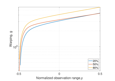
Figure 2: Learned warping transformations with WGP for different rates of training samples. The range of $y$ is normalized $[-1,1]$ for better representation.

III-B Experiment 2: Estimation of vegetation parameters

In this second experiment, we used data from the SPARC campaign acquired during the month of July of 2003 in Barrax (Spain), previously mentioned in Sec. II. We have in-situ ground-truth data of three different vegetation parameters, chlorophyll-a (Chl-a), Leaf Area Index (LAI) and Fraction of Vegetation Cover (FVC). We trained the models using hyperspectral reflectances from the CHRIS instrument on board of PROBA-1 satellite, which provides information in 62 spectral channels at a spatial resolution of about 34 meters.

As the number of training samples are scarce (only $n=135$ labeled samples in total), we report results using a $4$-fold cross validation procedure. The results in Table II show the mean and the standard deviation for the experiments. Results are reported in the same terms that in the previous experiment III-A. The proposed warped GP regression (WGP) obtains better results for prediction of Chl-a content and FVC. WGP achieves better quality estimates and lower error bars compared to the other GP models.

TABLE II: Bias (ME), accuracy (RMSE) and fitness (R²) for the tested vegetation variables (Chl-a, LAI, FVC) in the SPARC dataset.

	ME	RMSE	R2
Chl-a
GP	-0.99 $\pm$ 2.14	5.75 $\pm$ 3.81	0.845 $\pm$ 0.16
VHGP	-1.05 $\pm$ 2.15	5.58 $\pm$ 4.12	0.854 $\pm$ 0.17
WGP	-0.51 $\pm$ 1.89	5.16 $\pm$ 3.13	0.873 $\pm$ 0.12
LAI
GP	0.005 $\pm$ 0.10	0.53 $\pm$ 0.07	0.879 $\pm$ 0.03
VHGP	0.03 $\pm$ 0.15	0.55 $\pm$ 0.05	0.875 $\pm$ 0.03
WGP	0.02 $\pm$ 0.14	0.55 $\pm$ 0.11	0.867 $\pm$ 0.05
FVC
GP	0.012 $\pm$ 0.009	0.142 $\pm$ 0.040	0.796 $\pm$ 0.105
VHGP	-0.021 $\pm$ 0.013	0.144 $\pm$ 0.041	0.799 $\pm$ 0.088
WGP	0.006 $\pm$ 0.007	0.137 $\pm$ 0.038	0.814 $\pm$ 0.090

For illustration purposes, we show in Fig. 3 the prediction maps, confidence intervals and the ratio between them. The proposed WGP predicts in general lower values of Chl-a content, mostly in the center and eastern region of the scene, and provides a lower uncertainty in the whole image. On the contrary, GP and VHGP obtained low uncertainty only in the western area of the scene and high uncertainty on the central region. Actually, when looking at the ratio between the predictive mean and variance (third row), WGP obtained lower and more homogeneous results. The lower the ratio, the better the results are. We masked the ratio by fixing a threshold of 20%: GP provided only 52.21% of the predictions below this threshold, VHGP yielded a 69.72%, and WGP fulfilled this error for the whole image.

GP	VHGP	WGP

Figure 3: Prediction maps of chlorophyll-a content by GP, VHGP and WGP: predictive mean (top row), variance (middle) and coefficient of variation -ratios- (bottom) are represented.

III-C Experiment 3: Causal inference in geosciences

Establishing causal relations between random variables from observational data is perhaps the most important challenge in today’s Science. In remote sensing and geosciences this is of special relevance to better understand the Earth’s system and the complex interactions between the involved processes.

TABLE III: Problems and causal direction for the geoscience problems in the CEP database.

id	$x$	$y$	Cause
01	Altitude	Temperature	$\rightarrow$
02	Altitude	Precipitation	$\rightarrow$
03	Longitude	Temperature	$\rightarrow$
04	Altitude	Sunshine hours	$\rightarrow$
20	Latitude	Temperature	$\rightarrow$
21	Longitude	Precipitation	$\rightarrow$
42	Day of the year	Temperature	$\rightarrow$
43	Temperature at $t$	Temperature at $t+1$	$\rightarrow$
44	Pressure at $t$	Pressure at $t+1$	$\rightarrow$
45	Sea level pressure at $t$	Sea level pressure at $t+1$	$\rightarrow$
46	Relative humidity at $t$	Relative humidity at $t+1$	$\rightarrow$
49	Ozone concentration	Temperature	$\leftarrow$
50	Ozone concentration	Temperature	$\leftarrow$
51	Ozone concentration	Temperature	$\leftarrow$
72	Sunspots	Global mean temperature	$\rightarrow$
73	CO2 emissions	Energy use	$\leftarrow$
77	Temperature	Solar radiation	$\leftarrow$
78	PPFD	Net Ecosystem Productivity	$\rightarrow$
79	NEP	Diffuse PPFDdif	$\leftarrow$
80	NEP	Diffuse PPFDdif	$\leftarrow$
81	Temperature	Local CO2 flux, BE-Bra	$\rightarrow$
82	Temperature	Local CO2 flux, DE-Har	$\rightarrow$
83	Temperature	Local CO2 flux, US-PFa	$\rightarrow$
87	Temperature	Total snow	$\rightarrow$
89	root decomposition	root decomposition (grassland)	$\leftarrow$
90	root decomposition	root decomposition (forest)	$\leftarrow$
91	clay content in soil	soil moisture	$\rightarrow$
92	organic carbon in soil	clay cont. in soil (forest)	$\leftarrow$
93	precipitation	runoff	$\rightarrow$
94	hour of day	temperature	$\rightarrow$

In this experiment we used Version 1.0 of the CauseEffectPairs (CEP) collection. The database contains 100 pairs of random variables along with the right direction of causation (ground truth). Data has been collected from various domains of application, such as biology, climate science, health sciences and economics, to name a few [10]. We conducted experiments in 28 out of the 100 pairs that contain one-dimensional variables and that are related to geosciences and remote sensing: problems involving carbon and energy fluxes, ecological indicators, vegetation indices, temperature, moisture, heat, etc. We summarize the involved variables in Table III.

We build upon the framework proposed in [11] to derive cause-effect relations from pairs of random variables. The method decides about the causal direction based on the independence of the residuals with respect to the causal mechanism. Notationally, two regression models $\hat{y}=f(x)$ and $\hat{x}=g(y)$ are developed trying to estimate one variable from the other, and then two Hilbert Schmidt Independence Criterion (HSIC) [13] terms between the residuals $n_{f}=\hat{y}-f(x)$ (or $n_{b}=\hat{x}-g(y)$) and the corresponding potential cause $x$ (or $y$), respectively. The causal direction score is defined here as the difference in test statistic between both models [10]. For the regression models, we run standard GPs, VHGP and the proposed WGP, and measured independence with HSIC, which has been widely used in remote sensing as well for feature selection and dependence estimation [14]. Figure 4 shows the receiver operating curves (ROCs) for all GP models in the case of using a limited number of points $n=1000$ per problem. It can be noticed that all methods perform above chance, and that WGP performs better than the rest in area under the ROC.

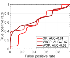
Figure 4: ROC for the identification of cause-effects in a subset of remote sensing and geosciences pairs using GP (AUC=0.61), VHGP (AUC=0.67) and the proposed WGP (AUC=0.68).

IV Conclusions

We introduced warped GPs for remote sensing and geoscience applications involving parameter estimation and causal inference from bivariate problems. WGP regression is able to learn an optimal transform. The introduced model generalizes standard GPs and allows to work with both non-Gaussian processes and non-Gaussian noise. Improved results in terms of accuracy were attained, more credible and tighter confidence intervals, and the advantage of deriving an optimal transform for further use. Results in several experiments suggest that WGPs are a solid approach to both quantitative and qualitative remote sensing data analysis because of the good accuracy and explanatory capabilities. Ongoing work is tied to learning both non-parametric functions following [15] on a full Bayesian treatment of warping.

References

- [1] C. E. Rasmussen and C. K. I. Williams, Gaussian Processes for Machine Learning, The MIT Press, New York, 2006.
- [2] J. Verrelst, L. Alonso, G. Camps-Valls, J. Delegido, and J. Moreno, “Retrieval of vegetation parameters using Gaussian processes techniques,” IEEE Trans. Geosc. Rem. Sens., vol. 49, pp. 1832–1843, 2012.
- [3] G. Camps-Valls, J. Verrelst, J. Muñoz Marí, V. Laparra, F. Mateo-Jiménez, and J. Gómez-Dans, “A survey on gaussian processes for earth observation data analysis: A comprehensive investigation,” IEEE Geoscience and Remote Sensing Magazine, June 2016.
- [4] David Duvenaud, James Robert Lloyd, Roger Grosse, Joshua B. Tenenbaum, and Zoubin Ghahramani, “Structure discovery in nonparametric regression through compositional kernel search,” in Proceedings of the 30th International Conference on Machine Learning, June 2013.
- [5] S. Salcedo-Sanz, C. Casanova-Mateo, J. Muñoz Marí, and G. Camps-Valls, “Prediction of daily global solar irradiation using temporal gaussian processes,” Geoscience and Remote Sensing Letters, IEEE, vol. 11, no. 11, pp. 1936–1940, Nov 2014.
- [6] David B. Dunson and Emily B. Fox, “Multiresolution gaussian processes,” in NIPS, F. Pereira, C.J.C. Burges, L. Bottou, and K.Q. Weinberger, Eds., pp. 737–745. Curran Associates, Inc., 2012.
- [7] M. Lázaro-Gredilla, M. K. Titsias, J. Verrelst, and G. Camps-Valls, “Retrieval of biophysical parameters with heteroscedastic gaussian processes,” IEEE Geosci. Remote Sensing Lett., vol. 11, no. 4, pp. 838–842, 2014.
- [8] E. Snelson, C. Rasmussen, and Z. Ghahramani, “Warped gaussian processes,” in NIPS. 2004, MIT Press.
- [9] J. E. O’Reilly, S. Maritorena, B. G. Mitchell, D. A. Siegel, K. Carder, S. A. Garver, M. Kahru, and C. McClain, “Ocean color chlorophyll algorithms for SeaWiFS,” Journal of Geophysical Research, vol. 103, no. C11, pp. 24937–24953, Oct 1998.
- [10] Joris M. Mooij, Jonas Peters, Dominik Janzing, Jakob Zscheischler, and Bernhard Schölkopf, “Distinguishing cause from effect using observational data: Methods and benchmarks,” Journal of Machine Learning Research, vol. 17, pp. 32:1–32:102, 2016.
- [11] Patrik O. Hoyer, Dominik Janzing, Joris M. Mooij, Jonas Peters, and Bernhard Schölkopf, “Nonlinear causal discovery with additive noise models,” in NIPS, D. Koller, D. Schuurmans, Y. Bengio, and L. Bottou, Eds., 2009, pp. 689–696.
- [12] Judea Pearl, Causality: Models, Reasoning and Inference, Cambridge University Press, New York, NY, USA, 2nd edition, 2009.
- [13] A. Gretton, R. Herbrich, and A. Hyvärinen, “Kernel methods for measuring independence,” Journal of Machine Learning Research, vol. 6, pp. 2075–2129, 2005.
- [14] G. Camps-Valls, J. Mooij, and B. Scholkopf, “Remote sensing feature selection by kernel dependence measures,” IEEE Geosc. Rem. Sens. Lett., vol. 7, no. 3, pp. 587 –591, Jul 2010.
- [15] Miguel Lázaro-Gredilla, “Bayesian warped gaussian processes,” in NIPS, 2012, pp. 1628–1636.