Centrality dependence of dilepton production via $\gamma\gamma$ processes from Wigner distributions of photons in nuclei

Abstract

We propose a new complete method, based on the Wigner distributions of photons, how to calculate differential distributions of dileptons created via photon-photon fusion in semicentral ($b<2R_{A}$) $AA$ collisions. The formalism is used to calculate different distributions of invariant mass, dilepton transverse momentum and acoplanarity for different regions of centrality. The results of calculation are compared with recent STAR, ALICE and ATLAS experimental data. Very good agreement with the data is achieved without free parameters and without including additional mechanisms such as a possible rescattering of leptons in the quark-gluon plasma.

I Introduction

Ultrarelativistic Heavy Ions of large charge $Z$ are accompanied by a large flux of Weizsäcker–Williams photons. This opens up the opportunity to study a variety of photoinduced nuclear processes, as well as photon-photon processes. See for example the reviews with focus on RHIC and LHC Baur:2001jj ; Bertulani:2005ru ; Contreras:2015dqa ; Klein:2020fmr ; Schafer:2020bnm . Until recently, most investigations have focused on ultraperipheral collisions, where the coherent enhancement $\propto Z^{2}$ of Weizsäcker-Williams fluxes is evident. Here the impact parameter of the collision satisfies $b>2R_{A}$, with $R_{A}$ being the nuclear radius. A prominent role play the dileptons created via photon-photon fusion, for recent calculations at collider kinematics, see for example KlusekGawenda:2010kx ; Azevedo:2019fyz .

However, if one interprets Weizsäcker-Williams photons as partons of the nucleus, it appears natural that the coherent photon cloud also contributes in semicentral or central collisions, where $b<2R_{A}$. In such collisions the colliding nuclei will interact strongly generating an ”underlying event” for the $\gamma\gamma$ process, which may include the production of a quark-gluon plasma (QGP). In fact, such contributions have long been suggested Baron:1993sk . First experimental evidence for the relevance of photoproduction processes in inelastic Heavy Ion reactions was reported by the ALICE collaboration Adam:2015gba . Indeed, the large enhancement of $J/\psi$ at low transverse momenta observed in Adam:2015gba can be readily explained through the presence of photoproduction mechanisms Klusek-Gawenda:2015hja .

It was realized only recently that also coherent photon-photon processes survive in semicentral collisions. Two years ago the STAR collaboration at RHIC Adam:2018tdm observed a large enhancement at very low transverse momenta of the dielectron pair, $P_{T}<150\,\rm{MeV}$ . This enhancement was interpreted soon as due to photon-photon fusion Klusek-Gawenda:2018zfz ; Klein:2018fmp ; Zha:2018tlq ; Li:2019sin . Dilepton production in heavy ion collisions is traditionally considered as a source of information on the properties of the QCD matter produced in the collision Tserruya:2009zt ; Rapp:2013nxa . Besides the contributions of medium-modified vector mesons and thermal radiation from the QGP, there are several other mechanisms of dilepton production in ultrarelativistic heavy ion collisions. These are conventionally subsumed as the hadronic cocktail contribution which involves essentially all sources in nucleon-nucleon collisions (Dalitz decays, vector meson production, Drell-Yan mechanism, semileptonic decays of pairs of mesons).

In Klusek-Gawenda:2018zfz we performed a comprehensive study of the interplay of all these mechanisms, highlighting the dominance of $\gamma\gamma$ processes at very low $P_{T}$. However, in Ref.Klusek-Gawenda:2018zfz , the $P_{T}$ distribution of di-electrons was obtained using a $k_{T}$-factorization method. In such an approach the distribution in $P_{T}$ is independent of the impact parameter (and therefore centrality), and only the normalization contains information on the latter.

In Zha:2018tlq ; Li:2019sin it has been proposed to use an approach that has been put forward long ago in Vidovic:1992ik . However the formalism presented in Vidovic:1992ik applies only to the impact parameter dependence of invariant mass distributions of dileptons, and cannot be readily employed in an ”unintegrated” form to yield transverse momentum distributions.

In Klein:2018fmp it was suggested that rescattering in QGP may lead to a broadening of the $P_{T}$ peak and acoplanarity distribution of dileptons.

In this paper we present a more complete approach that allows to calculate the centrality dependence of the $\gamma\gamma$ mechanism of dilepton production. It is based on so-called Wigner distributions . We present the formalism in the next section. Then we shall confront results of the new method with existing experimental data. Conclusions will close our paper.

II Centrality dependent cross section of dilepton production

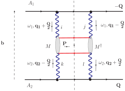
Figure 1: The cut off-forward $A_{1}A_{2}\to A_{1}A_{2}$ amplitude. Its Fourier transform w.r.t. $Q$ yields the impact-parameter dependent cross section of dilepton production.

For the ion moving at longitudinal boost $\gamma$, let us denote the electric field vector:

$$\mbox{\boldmath$E$}(\omega,\mbox{\boldmath$q$})=Z\sqrt{\frac{\alpha_{em}}{\pi}}\,{\mbox{\boldmath$q$}F_{\rm ch}(\mbox{\boldmath$q$}^{2}+q^{2}_{\parallel})\over\mbox{\boldmath$q$}^{2}+q^{2}_{\parallel}}\,,{\rm where}\,q_{\parallel}={\omega\over\gamma}\,,$$ (1)

and $F_{\rm ch}(Q^{2})$ is the charge form factor of the nucleus.

The impact parameter dependent cross section of interest is obtained from the Fourier transform of the cut off-forward $A_{1}A_{2}\to A_{1}A_{2}$ amplitude shown in Fig.1.

The relevant factorization formula can be written in terms of the Wigner function

$$N_{ij}(\omega,\mbox{\boldmath$b$},\mbox{\boldmath$q$}) = \int{d^{2}\mbox{\boldmath$Q$}\over(2\pi)^{2}}\,\exp[-i\mbox{\boldmath$b$}\mbox{\boldmath$Q$}]\,E_{i}\Big{(}\omega,\mbox{\boldmath$q$}+{\mbox{\boldmath$Q$}\over 2}\Big{)}E^{*}_{j}\Big{(}\omega,\mbox{\boldmath$q$}-{\mbox{\boldmath$Q$}\over 2}\Big{)}\,$$ (2)

$$= \int d^{2}\mbox{\boldmath$s$}\,\exp[i\mbox{\boldmath$q$}\mbox{\boldmath$s$}]\,E_{i}\Big{(}\omega,\mbox{\boldmath$b$}+{\mbox{\boldmath$s$}\over 2}\Big{)}E^{*}_{j}\Big{(}\omega,\mbox{\boldmath$b$}-{\mbox{\boldmath$s$}\over 2}\Big{)}.$$ (3)

It has the property of being a density matrix in photon polarizations (here we use the basis of cartesian linear polarizations), and depends on impact parameter and transverse momentum.

Being a Wigner function, the standard photon fluxes in momentum space and impact parameter space, are obtained after integration over impact parameter or momentum space, respectively, a summation over photon polarizations is implied:

$$N(\omega,\mbox{\boldmath$q$}) = \delta_{ij}\int d^{2}\mbox{\boldmath$b$}\,N_{ij}(\omega,\mbox{\boldmath$b$},\mbox{\boldmath$q$})=\delta_{ij}\,E_{i}(\omega,\mbox{\boldmath$q$})E^{*}_{j}(\omega,\mbox{\boldmath$q$})=\Big{|}\mbox{\boldmath$E$}(\omega,\mbox{\boldmath$q$})\Big{|}^{2}\,,$$

$$N(\omega,\mbox{\boldmath$b$}) = \delta_{ij}\int{d^{2}\mbox{\boldmath$q$}\over(2\pi)^{2}}N_{ij}(\omega,\mbox{\boldmath$b$},\mbox{\boldmath$q$})=\delta_{ij}\,E_{i}(\omega,\mbox{\boldmath$b$})E^{*}_{j}(\omega,\mbox{\boldmath$b$})=\Big{|}\mbox{\boldmath$E$}(\omega,\mbox{\boldmath$b$})\Big{|}^{2}\,.$$ (4)

Then the cross section for lepton pair production can be written as a convolution over impact parameters and transverse momenta

$${d\sigma\over d^{2}\mbox{\boldmath$b$}d^{2}\mbox{\boldmath$P$}} = \int d^{2}\mbox{\boldmath$b$}_{1}d^{2}\mbox{\boldmath$b$}_{2}\,\delta^{(2)}(\mbox{\boldmath$b$}-\mbox{\boldmath$b$}_{1}+\mbox{\boldmath$b$}_{2})\int{d^{2}\mbox{\boldmath$q$}_{1}\over\pi}{d^{2}\mbox{\boldmath$q$}_{2}\over\pi}\,\delta^{(2)}(\mbox{\boldmath$P$}-\mbox{\boldmath$q$}_{1}-\mbox{\boldmath$q$}_{2})$$ (5)

$$\times \int{d\omega_{1}\over\omega_{1}}{d\omega_{2}\over\omega_{2}}N_{ij}(\omega_{1},\mbox{\boldmath$b$}_{1},\mbox{\boldmath$q$}_{1})N_{kl}(\omega_{2},\mbox{\boldmath$b$}_{2},\mbox{\boldmath$q$}_{2})\,\,{1\over 2\hat{s}}\sum_{\lambda\bar{\lambda}}M^{\lambda\bar{\lambda}}_{ik}M^{\lambda\bar{\lambda}\dagger}_{jl}\,d\Phi(l^{+}l^{-}).$$

Here again we sum over cartesian photon polarizations $i,j,k,l$, and the invariant phase space of the leptons is:

$$d\Phi_{l^{+}l^{-}}=(2\pi)^{4}\,\delta^{(4)}(P-p_{1}-p_{2})\,{d^{4}p_{1}\over(2\pi)^{3}}\delta(p_{1}^{2}-m_{l}^{2}){d^{4}p_{2}\over(2\pi)^{3}}\delta(p_{2}^{2}-m_{l}^{2})\,.$$ (6)

We now parametrize

$$\mbox{\boldmath$b$}_{1}=\mbox{\boldmath$R$}+{\mbox{\boldmath$B$}\over 2},\,\,\mbox{\boldmath$b$}_{2}=\mbox{\boldmath$R$}-{\mbox{\boldmath$B$}\over 2}\,\Rightarrow d^{2}\mbox{\boldmath$b$}_{1}d^{2}\mbox{\boldmath$b$}_{2}=d^{2}\mbox{\boldmath$R$}\,d^{2}\mbox{\boldmath$B$}.$$ (7)

Below, we also use the notation $P_{T}\equiv|\mbox{\boldmath$P$}|$ for the transverse momentum of the dilepton pair. Inserting the representation of the generalized Wigner function given in Eq. (2) , and integrating out $R$ (the delta function puts $\mbox{\boldmath$b$}=\mbox{\boldmath$B$}$), we obtain

$${d\sigma\over d^{2}\mbox{\boldmath$b$}d^{2}\mbox{\boldmath$P$}} = \int{d^{2}\mbox{\boldmath$Q$}\over(2\pi)^{2}}\exp[-i\mbox{\boldmath$b$}\mbox{\boldmath$Q$}]\int{d^{2}\mbox{\boldmath$q$}_{1}\over\pi}{d^{2}\mbox{\boldmath$q$}_{2}\over\pi}\,\delta^{(2)}(\mbox{\boldmath$P$}-\mbox{\boldmath$q$}_{1}-\mbox{\boldmath$q$}_{2})\int{d\omega_{1}\over\omega_{1}}{d\omega_{2}\over\omega_{2}}$$ (8)

$$\times E_{i}\Big{(}\omega_{1},\mbox{\boldmath$q$}_{1}+{\mbox{\boldmath$Q$}\over 2}\Big{)}E^{*}_{j}\Big{(}\omega_{1},\mbox{\boldmath$q$}_{1}-{\mbox{\boldmath$Q$}\over 2}\Big{)}E_{k}\Big{(}\omega_{2},\mbox{\boldmath$q$}_{2}-{\mbox{\boldmath$Q$}\over 2}\Big{)}E^{*}_{l}\Big{(}\omega_{2},\mbox{\boldmath$q$}_{2}+{\mbox{\boldmath$Q$}\over 2}\Big{)}$$

$$\times {1\over 2\hat{s}}\sum_{\lambda\bar{\lambda}}M^{\lambda\bar{\lambda}}_{ik}M^{\lambda\bar{\lambda}\dagger}_{jl}\,d\Phi(l^{+}l^{-})\,.$$

Notice, that our approach predicts “flow-like” correlations between the dilepton transverse momentum and the impact parameter $b$. We defer the discussion of these correlations to a future publication, and in this work we will average over directions of $b$. The cross section in a certain centrality class is obtained by integrating over the corresponding range of impact parameters:

$$d\sigma[{\cal C}]=\int_{b_{\rm min}}^{b_{\rm max}}db\,{d\sigma\over db}\,.$$ (9)

If we are interested in the cross section in a certain centrality class ${\cal C}$, we can get rid of the integration over $d^{2}\mbox{\boldmath$b$}$. We start from integrating over all possible orientations of $b$.

$$\int d^{2}\mbox{\boldmath$b$}\exp[-i\mbox{\boldmath$b$}\mbox{\boldmath$Q$}](\dots)\rightarrow 2\pi\int dbbJ_{0}(bQ)(\dots)\,.$$ (10)

Integrating over a range $[b_{\rm min},b_{\rm max}]$ of impact parameters, we obtain

$$\int_{b_{\rm min}}^{b_{\rm max}}db\,bJ_{0}(bQ)={1\over Q^{2}}\Big{(}Qb_{\rm max}J_{1}(Qb_{\rm max})-Qb_{\rm min}J_{1}(Qb_{\rm min})\Big{)}\equiv w(Q;b_{\rm max},b_{\rm min})\,.$$ (11)

Thus the cross section for a certain centrality class $\cal C$ is:

$${d\sigma[{\cal C}]\over d^{2}\mbox{\boldmath$P$}} = \int{d^{2}\mbox{\boldmath$Q$}\over 2\pi}w(Q;b_{\rm max},b_{\rm min})\int{d^{2}\mbox{\boldmath$q$}_{1}\over\pi}{d^{2}\mbox{\boldmath$q$}_{2}\over\pi}\,\delta^{(2)}(\mbox{\boldmath$P$}-\mbox{\boldmath$q$}_{1}-\mbox{\boldmath$q$}_{2})\int{d\omega_{1}\over\omega_{1}}{d\omega_{2}\over\omega_{2}}$$ (12)

$$\times E_{i}\Big{(}\omega_{1},\mbox{\boldmath$q$}_{1}+{\mbox{\boldmath$Q$}\over 2}\Big{)}E^{*}_{j}\Big{(}\omega_{1},\mbox{\boldmath$q$}_{1}-{\mbox{\boldmath$Q$}\over 2}\Big{)}E_{k}\Big{(}\omega_{2},\mbox{\boldmath$q$}_{2}-{\mbox{\boldmath$Q$}\over 2}\Big{)}E^{*}_{l}\Big{(}\omega_{2},\mbox{\boldmath$q$}_{2}+{\mbox{\boldmath$Q$}\over 2}\Big{)}$$

$$\times {1\over 2\hat{s}}\sum_{\lambda\bar{\lambda}}M^{\lambda\bar{\lambda}}_{ik}M^{\lambda\bar{\lambda}\dagger}_{jl}\,d\Phi(l^{+}l^{-})\,.$$

The impact parameter intervals $[b_{\rm min},b_{\rm max}]$ corresponding to a given centrality class are obtained from a simple optical Glauber approach, as described in more detail in Klusek-Gawenda:2018zfz . Now, we come to the helicity structure of the $\gamma\gamma\to l^{+}l^{-}$ amplitude. Here, indices $i,j$ correspond to linear polarizations of photons, while $\lambda,\bar{\lambda}$ are the helicities of leptons. The amplitude takes the form (below $M(\lambda_{1}\lambda_{2},\lambda\bar{\lambda})$is the helicity amplitude for the $\gamma(\lambda_{1})\gamma(\lambda_{2})\to l^{-}(\lambda)l^{+}(\bar{\lambda})$ process):

$$M^{\lambda\bar{\lambda}}_{ik} = -{1\over 2}\Big{(}\hat{x}_{i}\hat{x}_{k}+\hat{y}_{i}\hat{y}_{k}\Big{)}\Big{(}M(++,\lambda\bar{\lambda})+M(--,\lambda\bar{\lambda})\Big{)}$$ (13)

$$-{i\over 2}\Big{(}\hat{x}_{i}\hat{y}_{k}-\hat{y}_{i}\hat{x}_{k}\Big{)}\Big{(}M(++,\lambda\bar{\lambda})-M(--,\lambda\bar{\lambda})\Big{)}$$

$$+{1\over 2}\Big{(}\hat{x}_{i}\hat{x}_{k}-\hat{y}_{i}\hat{y}_{k}\Big{)}\Big{(}M(-+,\lambda\bar{\lambda})+M(+-,\lambda\bar{\lambda})\Big{)}$$

$$+{i\over 2}\Big{(}\hat{x}_{i}\hat{y}_{k}+\hat{y}_{i}\hat{x}_{k}\Big{)}\Big{(}M(-+,\lambda\bar{\lambda})-M(+-,\lambda\bar{\lambda})\Big{)}\,.$$

Let us introduce the shorthand notation

$$M^{\lambda\bar{\lambda}}_{ik}=\delta_{ik}M^{(0,+)}_{\lambda\bar{\lambda}}-i\epsilon_{ik}M^{(0,-)}_{\lambda\bar{\lambda}}+P^{\parallel}_{ik}M^{(2,+)}_{\lambda\bar{\lambda}}+iP^{\perp}_{ik}M^{(2,-)}_{\lambda\bar{\lambda}}\,.$$ (14)

Here

$$\delta_{ik} = \hat{x}_{i}\hat{x}_{k}+\hat{y}_{i}\hat{y}_{k}\,,\,\epsilon_{ik}=\hat{x}_{i}\hat{y}_{k}-\hat{y}_{i}\hat{x}_{k}\,,P^{\parallel}_{ik}=\hat{x}_{i}\hat{x}_{k}-\hat{y}_{i}\hat{y}_{k}\,,\,P^{\perp}_{ik}=\hat{x}_{i}\hat{y}_{k}+\hat{y}_{i}\hat{x}_{k}\,.$$ (15)

Then, in the cross-section of interest, we need

$$\sum_{\lambda\bar{\lambda}}M_{ik}^{\lambda\bar{\lambda}}M_{jl}^{\lambda\bar{\lambda}\dagger} = \delta_{ik}\delta_{jl}\sum_{\lambda\bar{\lambda}}\Big{|}M^{(0,+)}_{\lambda\bar{\lambda}}\Big{|}^{2}+\epsilon_{ik}\epsilon_{jl}\sum_{\lambda\bar{\lambda}}\Big{|}M^{(0,-)}_{\lambda\bar{\lambda}}\Big{|}^{2}$$ (16)

$$+ P^{\parallel}_{ik}P^{\parallel}_{jl}\sum_{\lambda\bar{\lambda}}\Big{|}M^{(2,+)}_{\lambda\bar{\lambda}}\Big{|}^{2}+P^{\perp}_{ik}P^{\perp}_{jl}\sum_{\lambda\bar{\lambda}}\Big{|}M^{(2,-)}_{\lambda\bar{\lambda}}\Big{|}^{2}\,.$$

Here we decomposed the $\gamma\gamma\to l^{+}l^{-}$ amplitude into channels of total angular momentum projection $J_{z}=0,\pm 2$ and even and odd parity. The explicit expressions for the squares of amplitudes, in terms of cm-scattering angle $\theta$ read:

$$\sum_{\lambda\bar{\lambda}}\Big{|}M^{(0,+)}_{\lambda\bar{\lambda}}\Big{|}^{2} = g^{4}_{\rm em}{8(1-\beta^{2})\beta^{2}\over(1-\beta^{2}\cos^{2}\theta)^{2}}\,,\,$$

$$\sum_{\lambda\bar{\lambda}}\Big{|}M^{(0,-)}_{\lambda\bar{\lambda}}\Big{|}^{2} = g^{4}_{\rm em}{8(1-\beta^{2})\over(1-\beta^{2}\cos^{2}\theta)^{2}}\,,$$

$$\sum_{\lambda\bar{\lambda}}\Big{|}M^{(2,+)}_{\lambda\bar{\lambda}}\Big{|}^{2} = g^{4}_{\rm em}{8\beta^{2}\sin^{2}\theta\over(1-\beta^{2}\cos^{2}\theta)^{2}}\Big{(}1-\beta^{2}\sin^{2}\theta\Big{)}\,,$$

$$\sum_{\lambda\bar{\lambda}}\Big{|}M^{(2,-)}_{\lambda\bar{\lambda}}\Big{|}^{2} = g^{4}_{\rm em}{8\beta^{2}\sin^{2}\theta\over(1-\beta^{2}\cos^{2}\theta)^{2}}\,,$$ (17)

where $g^{2}_{\rm em}=4\pi\alpha_{\rm em}$, and

$$\beta=\sqrt{1-{4m_{l}^{2}\over M^{2}}}$$ (18)

is the lepton velocity in the dilepton cms-frame. Notice that in the ultrarelativistic limit $\beta\to 1$, the $|J_{z}|=2$ terms dominate, while for $\beta\ll 1$, relevant for heavy fermions, the $J_{z}=0$ components are the leading ones. A brief comment on the approach used in Ref.Klein:2020jom is in order: the helicity structure used for the hard $\gamma\gamma\to l^{+}l^{-}$ process in Klein:2020jom corresponds to the sum of our $|J_{z}|=2$ terms for $\beta\to 1$.

The phase space of the dileptons can be parametrized by the rapidities $y_{1,2}$ and transverse momenta $\mbox{\boldmath$p$}_{1},\mbox{\boldmath$p$}_{2}$ of leptons. Then the cross section fully differential in lepton variables is obtained as

$${d\sigma[{\cal C}]\over dy_{1}dy_{2}d^{2}\mbox{\boldmath$p$}_{1}d^{2}\mbox{\boldmath$p$}_{2}} = \int{d^{2}\mbox{\boldmath$Q$}\over 2\pi}w(Q;b_{\rm max},b_{\rm min})\int{d^{2}\mbox{\boldmath$q$}_{1}\over\pi}{d^{2}\mbox{\boldmath$q$}_{2}\over\pi}\,\delta^{(2)}(\mbox{\boldmath$p$}_{1}+\mbox{\boldmath$p$}_{2}-\mbox{\boldmath$q$}_{1}-\mbox{\boldmath$q$}_{2})$$ (19)

$$\times E_{i}\Big{(}\omega_{1},\mbox{\boldmath$q$}_{1}+{\mbox{\boldmath$Q$}\over 2}\Big{)}E^{*}_{j}\Big{(}\omega_{1},\mbox{\boldmath$q$}_{1}-{\mbox{\boldmath$Q$}\over 2}\Big{)}E_{k}\Big{(}\omega_{2},\mbox{\boldmath$q$}_{2}-{\mbox{\boldmath$Q$}\over 2}\Big{)}E^{*}_{l}\Big{(}\omega_{2},\mbox{\boldmath$q$}_{2}+{\mbox{\boldmath$Q$}\over 2}\Big{)}$$

$$\times {1\over 16\pi^{2}\hat{s}^{2}}\sum_{\lambda\bar{\lambda}}M^{\lambda\bar{\lambda}}_{ik}M^{\lambda\bar{\lambda}\dagger}_{jl}\,.$$

The delta-functions in the phase space element determine the photon energies as:

$$\omega_{1} = \frac{1}{2}\Big{(}m_{1t}\exp(+y_{1})+m_{2t}\exp(+y_{2})\Big{)}\,,\omega_{2}=\frac{1}{2}\Big{(}m_{1t}\exp(-y_{1})+m_{2t}\exp(-y_{2})\Big{)}\,.$$ (20)

where $m_{it}=\sqrt{\mbox{\boldmath$p$}_{i}^{2}+m_{l}^{2}}$. We perform the multidimensional integration using the VEGAS Monte Carlo method Lepage:1977sw .

III Results of the new approach versus experimental data

In this section we present predictions for the centrality dependence of $l^{+}l^{-}$ production Au-Au collisions at RHIC energy ($\sqrt{s_{NN}}$=200 GeV) and Pb-Pb collisions at LHC energy ($\sqrt{s_{NN}}$=5.02 TeV). The results of our approach will be compared to STAR, ALICE and ATLAS experimental data.

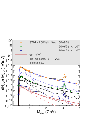
(a) (b)

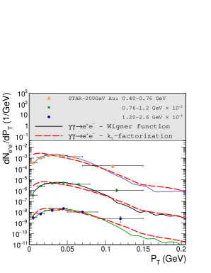
Figure 2: Theoretical predictions vs. STAR experimental data at RHIC energy ($\sqrt{s}$ = 200 GeV) Adam:2018tdm . (a) Dielectron invariant mass spectra for three ranges of centrality: 60 - 80 % (upper curve), 40 - 60 % (middle curve) and 10 - 40 % (lower curve) Adam:2018tdm . Thermal radiation (dotted lines) and hadronic cocktail (dashed lines) contributions are compared with $\gamma\gamma\to e^{+}e^{-}$ process Klusek-Gawenda:2018zfz . (b) Distribution of transverse momentum of dielectron pair for three invariant mass limits Adam:2018tdm . $k_{T}$-factorization result (dashed lines) Klusek-Gawenda:2018zfz is shown for comparison to the new results (solid lines). The centrality is in the limit: (60-80)$\%$

We start the presentation of our results from the invariant mass distribution of low-$P_{T}$ dielectrons. In Fig.2(a) we show our $\gamma\gamma$-fusion results (solid lines) together with the STAR experimental data Adam:2018tdm for three different ranges of centrality as defined in the STAR experiment. The calculation of the invariant mass distribution reproduces very well the results of our earlier work Klein:2018fmp . The photon-photon process dominates for peripheral collisions. For the most central collisions, (10 - 40 )%, the $\gamma\gamma$ process starts to underestimate the experimental data. The detailed discussion of thermal radiation and hadronic cocktail is found in Klusek-Gawenda:2018zfz and must not be repeated here. We stress that the theoretical results are calculated including STAR experimental cuts i.e. $p_{t,e}>0.2$ GeV, $|\eta_{e}|<1$, $|y_{e^{+}e^{-}}|<1$ and $P_{T}<0.15$ GeV.

In Fig.2(b) we show the distribution in transverse momentum of the dielectron pairs for three centrality intervals. We get very good description of the low-$P_{T}$ enhancement, within the newly presented approach.

In our previous work Klusek-Gawenda:2018zfz we calculated the $P_{T}$-distribution in what we dub a $k_{T}$-factorization approach, where the transverse momentum of dileptons involves a convolution of the $q$-dependent photon fluxes, schematically:

$$N_{l^{+}l^{-}}(\mbox{\boldmath$P$})\propto\int{d\omega_{1}\over\omega_{1}}{d\omega_{2}\over\omega_{2}}\int{d^{2}\mbox{\boldmath$q$}_{1}\over\pi}{d^{2}\mbox{\boldmath$q$}_{2}\over\pi}\delta^{(2)}(\mbox{\boldmath$P$}-\mbox{\boldmath$q$}_{1}-\mbox{\boldmath$q$}_{2})N(\omega_{1},\mbox{\boldmath$q$}_{1})N(\omega_{2},\mbox{\boldmath$q$}_{2})\sigma_{\gamma\gamma\to l^{+}l^{-}}(4\omega_{1}\omega_{2})\,.$$

(21)

While our previous calculations in Klusek-Gawenda:2018zfz convincingly demonstrated the dominance of the $\gamma\gamma$ process at low $P_{T}$, the peak of the distribution obtained from Eq. (21) is systematically at too low values of $P_{T}$, and neglects the correlation of $P_{T}$ with centrality.

Our new theoretical results give an excellent description of both the shape and normalization of the low-$P_{T}$ enhancement. In our approach here we use a charge form factor of the nucleus obtained from a realistic charge distribution described in KlusekGawenda:2010kx . The form factor almost coincides with the one used in STARlight simulation code Klein:2016yzr .

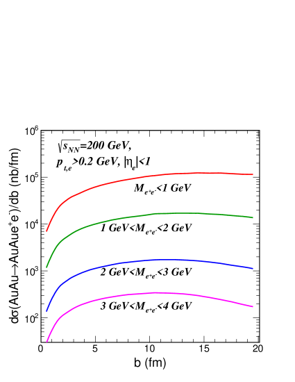
Figure 3: Impact parameter dependence for $\sqrt{s_{NN}}$ = 200 GeV and different windows of dielectron invariant mass.

For completeness, in Fig.3 we show cross section for the $AuAu\to e^{+}e^{-}AuAu$ process as a function of impact parameter. Here we have taken kinematical cuts adequate for the STAR experiment. We note that the shape in impact parameter depends on the window of dielectron mass. The impact parameter cannot be directly measured. As previously done in Klusek-Gawenda:2018zfz , we use an optical Glauber model Miller:2007ri to estimate geometric quantities. For normalization we need the total hadronic inelastic cross section. We use the following values of cross sections: $\sigma_{AuAu}(\sqrt{s_{NN}}=200~{}\mbox{GeV})=6\,936$ mb and $\sigma_{PbPb}(\sqrt{s_{NN}}=5.02~{}\mbox{TeV})=7\,642$ mb.

We now proceed to LHC energies. In Fig. 4 we show our results compared to the preliminary experimental results obtained by the ALICE collaboration Lehner:2019amb . We get a similarly good description of the preliminary ALICE data as for the case of the STAR data. For illustration we show also result of the $k_{T}$-factorization (dashed line) proposed in Klusek-Gawenda:2018zfz , which clearly fails to describe the position of the peak. Indeed, the peak of the $P_{T}$ distribution predicted by the $k_{T}$-factorization formula Eq. (21) runs away towards smaller and smaller $P_{T}$ with increasing energy. This is related to the fact, that in the photon distribution

$$N(\omega,\mbox{\boldmath$q$})\propto|\mbox{\boldmath$E$}(\omega,\mbox{\boldmath$q$})|^{2}\propto{\mbox{\boldmath$q$}^{2}\over[\mbox{\boldmath$q$}^{2}+(\omega/\gamma)^{2}]^{2}}F^{2}_{\rm{ch}}(\mbox{\boldmath$q$}^{2}+(\omega/\gamma)^{2})\,,$$ (22)

the “cutoff” $\omega/\gamma$ decreases with increasing cm-energy (or boost $\gamma$ of the ion).

Consequently, for the much lower STAR energies the $k_{T}$-factorization approach is only slightly worse than that in the new approach (see Fig. 2(b)).

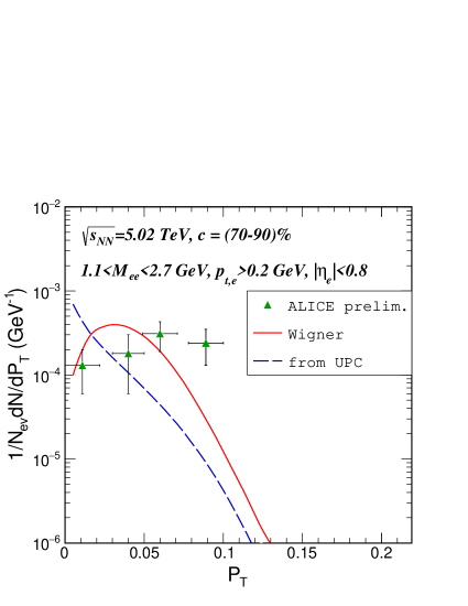
Figure 4: Distribution in transverse momentum of the dielectron pair for $\sqrt{s}$ = 5.02 TeV. The results of the present approach is shown by the solid line. The preliminary ALICE data Lehner:2019amb are shown for comparison.

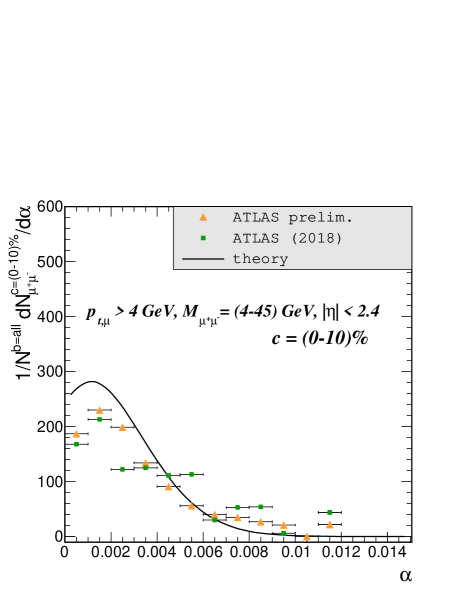
Figure 5: Acoplanarity distribution for $\mu^{+}\mu^{-}$ production for the kinematics of the ATLAS experiment. For comparison we show preliminary results ATLAS:2019vxg as well as previously published ones Aaboud:2018eph .

Finally in Fig.5 we show the acoplanarity distribution for dimuon production as measured by the ATLAS collaboration Aaboud:2018eph ; ATLAS:2019vxg . The acoplanarity is defined as:

$$\alpha=1-{|\Delta\phi_{l^{+}l^{-}}|\over\pi}\;,$$ (23)

where $\Delta\phi_{l^{+}l^{-}}$ is the difference of the azimuthal angles of two leptons. The measurement of the dimuon production via $\gamma\gamma$ scattering process was done at rather large transverse momenta ($p_{t,\mu}>4$ GeV) of leptons. Our previous study of semi-central collisions at the LHC Klusek-Gawenda:2018zfz has shown that the dilepton invariant mass (up to $1.5$ GeV) thermal radiation occurs only at centrality smaller than 50 %. Consequently, we obtain a successful description of data by $\gamma\gamma$-fusion alone for the high invariant mass even for low centrality. Our result is also in surprisingly good agreement for the case of very central collisions ($c=(0-10)\%$). Here we get better agreement with the new preliminary data.

In Fig. 6 we show the results for nine different centrality intervals, from central up to peripheral heavy-ion collision. We have got a very nice description of the data including correct normalization and shape of the distributions. At larger acoplanarity there is a long tail possibly due to soft photon emission Klein:2020jom . This tail cannot be, however, seen in the linear scale used here and is not included in our calculation.

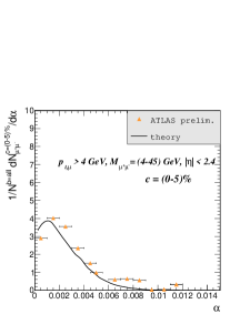
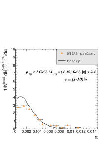
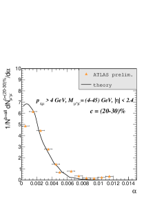
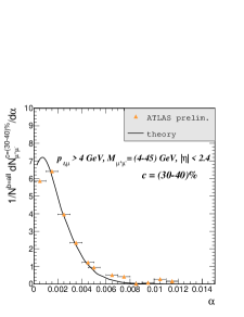
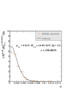
Figure 6: Acoplanarity distribution for $\mu^{+}\mu^{-}$ production for the kinematics of the ATLAS experiment Aaboud:2018eph ; ATLAS:2019vxg . The solid line represents result of the approach presented in this paper. Each panel corresponds to a different centrality class.

IV Conclusion

In this paper we have presented a formalism how to calculate differential distributions of leptons produced in semi-central ($b<2R_{A}$) nucleus-nucleus collisions for a given centrality. In this approach the differential cross section is calculated using the complete polarization density matrix of photons resulting from the Wigner distribution formalism.

We have presented results of calculation of several differential distributions such as invariant mass of dileptons, dilepton transverse momentum and acoplanarity for different regions of centrality. The results of the calculations have been compared to experimental data of the STAR, ALICE and ATLAS collaboration. A good agreement has been achieved in all cases. Our approach gives much better agreement with experimental data than the previous approaches used in the literature. Recently the CMS collaboration measured modifications of $\alpha$ distributions Sirunyan:2020vvm correlated with neutron multiplicity. A very new ATLAS study also presents the dimuon cross sections in the presence of forward and/or backward neutron production Aad:2020dur . This goes beyond present studies, and we plan such studies it in the future. Our formalism can be readily extended to such processes, using the impact parameter distributions obtained in Klusek-Gawenda:2013ema .

We have obtained a good description of the data without introducing additional final state rescattering of leptons in the quark-gluon plasma. More work is necessary to identify observables that can probe electromagnetic properties of the QGP.

References

- (1) Gerhard Baur, Kai Hencken, Dirk Trautmann, Serguei Sadovsky, and Yuri Kharlov. Coherent gamma gamma and gamma-A interactions in very peripheral collisions at relativistic ion colliders. Phys. Rept., 364:359–450, 2002. arXiv:hep-ph/0112211, doi:10.1016/S0370-1573(01)00101-6.
- (2) Carlos A. Bertulani, Spencer R. Klein, and Joakim Nystrand. Physics of ultra-peripheral nuclear collisions. Ann. Rev. Nucl. Part. Sci., 55:271–310, 2005. arXiv:nucl-ex/0502005, doi:10.1146/annurev.nucl.55.090704.151526.
- (3) J.G. Contreras and J.D. Tapia Takaki. Ultra-peripheral heavy-ion collisions at the LHC. Int. J. Mod. Phys. A, 30:1542012, 2015. doi:10.1142/S0217751X15420129.
- (4) Spencer Klein and Peter Steinberg. Photonuclear and Two-photon Interactions at High-Energy Nuclear Colliders. Ann.Rev.Nucl.Part.Sci., 70:232, 2020. arXiv:2005.01872, doi:10.1146/annurev-nucl-030320-033923.
- (5) Wolfgang Schäfer. Photon induced processes: from ultraperipheral to semicentral heavy ion collisions. Eur. Phys. J. A, 56(9):231, 2020. doi:10.1140/epja/s10050-020-00231-8.
- (6) M. Klusek-Gawenda and A. Szczurek. Exclusive muon-pair productions in ultrarelativistic heavy-ion collisions – realistic nucleus charge form factor and differential distributions. Phys. Rev. C, 82:014904, 2010. arXiv:1004.5521, doi:10.1103/PhysRevC.82.014904.
- (7) C. Azevedo, V.P. Gonçalves, and B.D. Moreira. Exclusive dilepton production in ultraperipheral collisions at the LHC. Eur. Phys. J. C, 79(5):432, 2019. arXiv:1902.00268, doi:10.1140/epjc/s10052-019-6952-8.
- (8) N. Baron and G. Baur. Unraveling gamma gamma dileptons in central relativistic heavy ion collisions. Z. Phys. C, 60:95–100, 1993. doi:10.1007/BF01650434.
- (9) Jaroslav Adam et al. Measurement of an excess in the yield of at very low in Pb-Pb collisions at = 2.76 TeV. Phys. Rev. Lett., 116(22):222301, 2016. arXiv:1509.08802, doi:10.1103/PhysRevLett.116.222301.
- (10) Mariola Kłusek-Gawenda and Antoni Szczurek. Photoproduction of mesons in peripheral and semicentral heavy ion collisions. Phys. Rev. C, 93(4):044912, 2016. arXiv:1509.03173, doi:10.1103/PhysRevC.93.044912.
- (11) Jaroslav Adam et al. Low- pair production in AuAu collisions at = 200 GeV and UU collisions at = 193 GeV at STAR. Phys. Rev. Lett., 121(13):132301, 2018. arXiv:1806.02295, doi:10.1103/PhysRevLett.121.132301.
- (12) Mariola Kłusek-Gawenda, Ralf Rapp, Wolfgang Schäfer, and Antoni Szczurek. Dilepton Radiation in Heavy-Ion Collisions at Small Transverse Momentum. Phys. Lett. B, 790:339–344, 2019. arXiv:1809.07049, doi:10.1016/j.physletb.2019.01.035.
- (13) Spencer Klein, A.H. Mueller, Bo-Wen Xiao, and Feng Yuan. Acoplanarity of a Lepton Pair to Probe the Electromagnetic Property of Quark Matter. Phys. Rev. Lett., 122(13):132301, 2019. arXiv:1811.05519, doi:10.1103/PhysRevLett.122.132301.
- (14) Wangmei Zha, James Daniel Brandenburg, Zebo Tang, and Zhangbu Xu. Initial transverse-momentum broadening of Breit-Wheeler process in relativistic heavy-ion collisions. Phys. Lett. B, 800:135089, 2020. arXiv:1812.02820, doi:10.1016/j.physletb.2019.135089.
- (15) Cong Li, Jian Zhou, and Ya-Jin Zhou. Impact parameter dependence of the azimuthal asymmetry in lepton pair production in heavy ion collisions. Phys. Rev. D, 101(3):034015, 2020. arXiv:1911.00237, doi:10.1103/PhysRevD.101.034015.
- (16) Itzhak Tserruya. Electromagnetic Probes. Landolt-Bornstein, 23:176, 2010. arXiv:0903.0415, doi:10.1007/978-3-642-01539-7_7.
- (17) Ralf Rapp. Dilepton Spectroscopy of QCD Matter at Collider Energies. Adv. High Energy Phys., 2013:148253, 2013. arXiv:1304.2309, doi:10.1155/2013/148253.
- (18) M. Vidovic, M. Greiner, C. Best, and G. Soff. Impact parameter dependence of the electromagnetic particle production in ultrarelativistic heavy ion collisions. Phys. Rev. C, 47:2308–2319, 1993. doi:10.1103/PhysRevC.47.2308.
- (19) Spencer Klein, A.H. Mueller, Bo-Wen Xiao, and Feng Yuan. Lepton Pair Production Through Two Photon Process in Heavy Ion Collisions. 3 2020. arXiv:2003.02947.
- (20) G.Peter Lepage. A New Algorithm for Adaptive Multidimensional Integration. J. Comput. Phys., 27:192, 1978. doi:10.1016/0021-9991(78)90004-9.
- (21) Spencer R. Klein, Joakim Nystrand, Janet Seger, Yuri Gorbunov, and Joey Butterworth. STARlight: A Monte Carlo simulation program for ultra-peripheral collisions of relativistic ions. Comput. Phys. Commun., 212:258–268, 2017. arXiv:1607.03838, doi:10.1016/j.cpc.2016.10.016.
- (22) Michael L. Miller, Klaus Reygers, Stephen J. Sanders, and Peter Steinberg. Glauber modeling in high energy nuclear collisions. Ann. Rev. Nucl. Part. Sci., 57:205–243, 2007. arXiv:nucl-ex/0701025, doi:10.1146/annurev.nucl.57.090506.123020.
- (23) Sebastian Lehner. Dielectron production at low transverse momentum in Pb-Pb collisions at TeV with ALICE. PoS, LHCP2019:164, 2019. arXiv:1909.02508, doi:10.22323/1.350.0164.
- (24) Measurement of non-exclusive dimuon pairs produced via scattering in Pb+Pb collisions at TeV with the ATLAS detector. ATLAS-CONF-2019-051.
- (25) Morad Aaboud et al. Observation of centrality-dependent acoplanarity for muon pairs produced via two-photon scattering in Pb+Pb collisions at TeV with the ATLAS detector. Phys. Rev. Lett., 121(21):212301, 2018. arXiv:1806.08708, doi:10.1103/PhysRevLett.121.212301.
- (26) Albert M Sirunyan et al. Observation of forward neutron multiplicity dependence of dimuon acoplanarity in ultraperipheral PbPb collisions at 5.02 TeV. 11 2020. arXiv:2011.05239.
- (27) Georges Aad et al. Exclusive dimuon production in ultraperipheral Pb+Pb collisions at TeV with ATLAS. 11 2020. arXiv:2011.12211.
- (28) Mariola Kłusek-Gawenda, Michał Ciemała, Wolfgang Schäfer, and Antoni Szczurek. Electromagnetic excitation of nuclei and neutron evaporation in ultrarelativistic ultraperipheral heavy ion collisions. Phys. Rev. C, 89(5):054907, 2014. arXiv:1311.1938, doi:10.1103/PhysRevC.89.054907.