Mass classification of dark matter perturbers of stellar tidal streams

Abstract

Stellar streams formed by tidal stripping of progenitors orbiting around the Milky Way are expected to be perturbed by encounters with dark matter subhalos. Recent studies have shown that they are an excellent proxy to infer properties of the perturbers, such as their mass. Here we present two different methodologies that make use of the fully non-Gaussian density distribution of stellar streams: a Bayesian model selection based on the probability density function (PDF) of stellar density, and a likelihood-free gradient boosting classifier. While the schemes do not assume a specific dark matter model, we are mainly interested in discerning the primordial black holes cold dark matter (PBH CDM) hypothesis form the standard particle dark matter one. Therefore, as an application we forecast model selection strength of evidence for cold dark matter clusters of masses $10^{3}$–$10^{5}M_{\Sun}$ and $10^{5}$–$10^{9}M_{\Sun}$, based on a GD-1-like stellar stream and including realistic observational errors. Evidence for the smaller mass range, so far under-explored, is particularly interesting for PBH CDM. We expect weak to strong evidence for model selection based on the PDF analysis, depending on the fiducial model. Instead, the gradient boosting model is a highly efficient classifier (99% accuracy) for all mass ranges here considered. As a further test of the robustness of the method, we reach similar conclusions when performing forecasts further dividing the largest mass range into $10^{5}$–$10^{7}M_{\Sun}$ and $10^{7}$–$10^{9}M_{\Sun}$ ranges.

1 Introduction

The nature of dark matter (DM) remains one of the most elusive mysteries of modern cosmology. While the existence of dark matter can be inferred from multiple observations, from the CMB to dwarf galaxies, its mass and interactions, even its corpuscular-versus-wave nature, is still unknown. In the last few years a new contender, primordial black holes (PBH) dark matter, see e.g. [1], has been reborn thanks to the LIGO detection of GW from massive BBH coalescence [2]. Their origin from the collapse of primordial fluctuations is rather generic [3], but their mass range and clustering properties are mostly uncertain. Some scenarios predict large non-Gaussian tails in the matter density contrast distribution that could give rise to clusters of PBH [4], thus evading all of the observational constraints [5, 6]. The abundance, size and mass of these clusters is rather model dependent. What we can infer from N-body simulations is their density profile and their spatial distribution over the halos of galaxies [7]. Their behaviour on large scales is indistinguishable from that of the usual collisionless dark matter components of cosmological N-body simulations that agree remarkably well with cosmological observations [8]. What differs from the usual particle dark matter (PDM) scenario is the small scale structure, and particularly the abundance and properties of subhalos with masses below $10^{6}~{}M_{\odot}$. Many of these PBH clusters evaporate via slingshot effects over the age of the universe, leaving dense cores of $10^{3}~{}M_{\odot}$ [7]. These small-mass PBH clusters orbit around the galaxy and interact with other collapsed objects like globular clusters and dwarf galaxies (see [9] for a prospective analysis constraining such interactions via trajectory intersections with Milky Way hyper-velocities stars). When these are tidally stretched by successive passages through the disk of the galaxy, they become what is known as tidal streams, almost one-dimensional concentrations of stars that stretch across the sky [10, 11, 12]. These highly-extended stellar streams are excellent targets for dark compact clusters of stars or black holes orbiting the central halo of the galaxy [13, 14, 15]. In this work we explore the possibility to distinguish and classify by mass the different perturbers that populate the galactic halo. In the future we may add to this analysis their size and concentration. Our ability to distinguish low-mass from high-mass clusters will then allow us to obtain information about the nature of dark matter. For instance, both Fuzzy DM and Warm DM predict that the smallest compact structures should have masses of order $10^{7}~{}M_{\odot}$, while axion miniclusters are typically in the range of $10^{-9}~{}M_{\odot}$. While PDM is expected to cluster down to $10^{-6}~{}M_{\odot}$ [16], we don’t expect a peak abundance of DM clusters in the $10^{3}-10^{5}~{}M_{\odot}$ range. Therefore, a detection of density perturbations in stellar streams suggesting an excess of subhalos compared to PDM would be an indication of the PBH nature of DM. On the other hand, these intermediate mass scales are too small to be detected by strong gravitational lensing effects on the light of distant galaxies and too large to significantly affect the microlensing of nearby stars. Therefore, we propose these methods as a new way to explore the nature of DM.

A convolutional neural network was built by [17] to classify DM subhalo masses based on Milky Way stars phase-space dynamics, expecting to be able to constrain masses down to $10^{7}M_{\Sun}$ in the near future. This lower limit is set in large part by the complicated stellar physics around the disk. In this work we focus on the Milky Way halo, and study stellar tidal stream dynamics in a regime where perturbation theory in the action-angle representation of streams applies [18]. The simplified picture allows us to reach high classification accuracy even for lower masses.

The density power spectrum of tidal streams was then studied by [18, 19, 20, 21, 14, 22], constraining the properties of perturbers for the Palomar 5 and GD-1 streams. [18] showed that not only the density, but also the mean track power spectrum and their bispectra contain important complementary information. The bispectrum is sensitive to profile asymmetries that are missed by the power spectrum. Given the non-Gaussian nature of density profiles, higher order correlation functions are likely to contain relevant information. Furthermore, given the computational requirements needed to estimate the Bayesian evidence based on the power spectrum, literature results relied on approximate Bayesian computations. [23] proposed a likelihood-free Bayesian inference pipeline built upon neural networks that avoids possibly insufficient summary statistic. In this work we also aim at profiting from the fully non-Gaussian information of stellar streams density profiles using machine learning techniques, but also a much simpler Bayesian approach.

[15, 24] showed that the gaps and the spur observed in GD-1 are consistent with having originated from a collision with a single massive perturber, see also [25] and  [26]. In this work we use a simulated GD-1-like tidal stream allowing the possibility of several impacts. Indeed, multiple impacts are expected in the standard cold dark matter (CDM) scenario, which for a GD-1-like stream amount to $\sim 60$ for perturbers in the range of masses $10^{5}$–$10^{9}M_{\Sun}$ [27]. This approach has the advantage of profiting from information coming not only from manifest features like large gaps, but from the full star distribution within the stream.

We present two novel methodologies aimed at constraining the mass of stellar streams dark matter perturbers. First, we outline a Bayesian model selection pipeline based on the PDF of stellar streams density perturbations. The PDF is a straightforward observable that takes into account the fully non-Gaussian information of density perturbations. For instance, it has been proven to be a valuable tool to model non-Gaussian statistics in Large Scale Structure studies [28, 29, 30, 31, 32], competitive but less computationally requiring than standard analyses based on correlation functions. Second, we consider a very different and complementary approach by training a gradient boosting classifier. As an application, we run simulations consistent with GD-1-like tidal stream and we forecast the possibility of selecting which one between different perturber mass ranges is favored by data. We consider a small $10^{3}$–$10^{5}M_{\Sun}$, and a large $10^{5}$–$10^{9}M_{\Sun}$ mass range. The smallest mass range is so far unexplored and motivated by the fact that it is suitable to test the PBH CDM scenario which is more likely to form subhalo objects of such masses than vanilla CDM [1]. Given uncertainties in the theoretical modeling of PBH, as a further test for the discriminating power of the analyses we also discuss results obtained splitting the largest mass range into two $10^{5}$–$10^{7}M_{\Sun}$ and $10^{7}$–$10^{9}M_{\Sun}$ ranges. This analysis will motivate future studies based on the specific statistical differences between PBH CDM and other DM models over the full $10^{3}$–$10^{9}M_{\Sun}$ mass range.

In section 2 we describe our simulated stellar streams. In section 3 we outline the two methodologies proposed to constrain DM clusters masses and show results in section 4. We conclude in section 5. A discusses convergence properties for our simulations. B considers the power spectrum of the streams and its limitations for a model selection analysis.

2 Simulations

We model a smooth GD-1-like tidal stream relying on the line-of-parallel-angle approach developed in [18], based on the action-angle representation of streams [33, 34]. In this formalism statistical properties of cold streams are well described by the density $\rho$ and mean track of parallel frequency $\langle\Omega_{\parallel}\rangle$ (average frequency along the stream) as a function the angle offset $\Delta\theta_{\parallel}$ (parallel to the direction along which the stream stretches) from the progenitor. The transformation from angle-frequency space in the neighbourhood of the stream to observable configuration space can be computed efficiently [33], allowing to assess the effect of observational errors.

Numerical simulations rely on galpy [35] and its extension streamgap-pepper [18]. Statistical sampling of multiple impacts follows section 2.3 of [18] to which we refer for more details and that here we only briefly review focusing on aspects that are relevant when considering PBH CDM perturbers rather than vanilla CDM. We neglect perturbations induced by baryonic structures as they are expected to be subdominant for a GD-1-like stream [23]. The following quantities are sampled sequentially:

1. Impact time $t_{i}$. We sample 64 values of time, corresponding to an interval of $\sim 140$ Myr (smaller than the radial period $\sim 400$ Myr of the stream) given the 9 Gyr age of the stream.

2. Angular offset $\Delta\theta_{i\parallel}$from the progenitor of closest approach along the stream.

3. Fly-by velocity ${\bf w}$ of the perturber, assuming a Gaussian distribution of CDM subhalos with dispersion $\sigma_{h}$ [27]).

4. Mass $M$ and internal structure of the perturber. The internal profile is described by the scale parameter $r_{s}$ of an Hernquist profile (see A for more details and a comparison with a Plummer profile). The mass $M$ probability distribution is taken to be $p(M)\propto r_{s}(M)dn_{h}/dM$, where we further assume a CDM subhalo spectrum $dn_{h}/dM\propto M^{-2}$ [37] and a scale factor obeying the deterministic relation $r_{s}(M)\propto M^{0.5}$ [38].

5. Impact parameter $b$, uniformly sampled along the diameter of a cylindrical volume with radius $b_{\rm max}$ around the stream [27]. Setting the radius proportional to the scale parameter, $b_{\rm max}=Xr_{s}$, takes effectively into account that decreasing the perturber mass also the volume of interaction decreases. We set $X=5$ as a compromise between computational convenience and numerical convergence of results (see A).

6. Number of impacts since the beginning of stream disruption to today, sampled from a Poisson distribution given the expected number $N_{i}=\sqrt{\frac{\pi}{2}}r_{\rm avg}\sigma_{h}t_{d}^{2}\Delta\Omega^{m}b_{\rm max}n_{h}$, where $r_{\rm avg}$ is the average spherical radius of the stream, $t_{d}$ is the time corresponding to the start of the stream disruption, $\Delta\Omega^{m}$ is the mean parallel frequency parameter of the smooth stream, and $n_{h}$ is the number of CDM sub-halos in the given mass range, estimated by extrapolating results compatible with the Via Lactea II simulation in the $10^{6}$–$10^{7}$ mass range [37, 18]. Given the reference impact parameter factor $X=5$, this brings $n_{h}\sim 839$ and $n_{h}\sim 62$ in the $10^{3}$–$10^{5}M_{\Sun}$ and $10^{5}$–$10^{9}M_{\Sun}$ mass ranges of our interest, respectively.

Note that the effect of the dark matter encounters are well modeled in the impulse approximation as instantaneous velocity kicks [18], neglecting effects of the collision on the perturber properties. To summarize, we sample from the following probability distribution:

$$\begin{split}p(t_{i},\Delta\theta_{i\parallel},{\bf w},M,r_{s},b,N_{i})=&\ p(t_{i})\ p(\Delta\theta_{i\parallel}|t_{i})\ p({\bf w}|t_{i},\Delta\theta_{i\parallel})\\ &p(M,r_{s}|t_{i},\Delta\theta_{i\parallel},{\bf w})\\ &p(b|t_{i},\Delta\theta_{i\parallel},{\bf w},M,r_{s})\\ &p(N_{i}|t_{i},\Delta\theta_{i\parallel},{\bf w},M,r_{s},b)\end{split}$$ (1)

For each sample we retrieve the density profile as a function of the parallel angle offset from the progenitor $\Delta\theta_{\parallel}$.

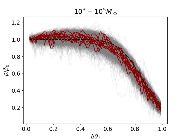
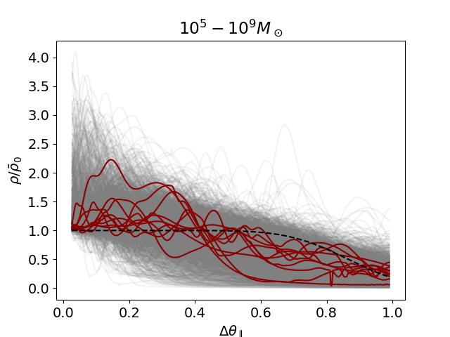
Figure 1: Simulated density profiles as a function of the parallel angle offset from the progenitor for different perturbers mass ranges. Dashed lines are the smooth density profiles. Grey lines are the perturbed density profiles. Red lines are a random selection of the latter with the purpose of visually distinguish a few full profiles.

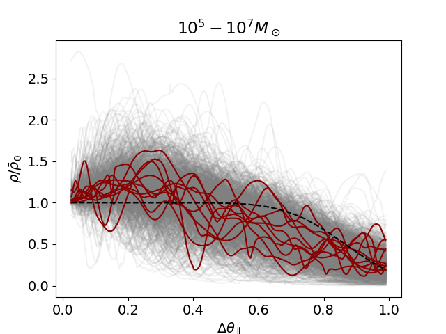
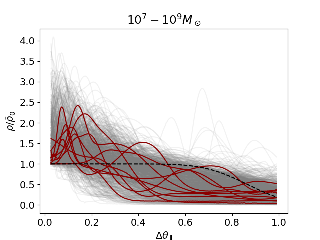
Figure 2: Like Figure 1, but separating the large mass range $10^{5}$–$10^{9}M_{\Sun}$ into two classes.

We compute at least 1000 samples of perturbed density profiles for each mass range $10^{3}$–$10^{5}M_{\Sun}$, $10^{5}$–$10^{9}M_{\Sun}$, shown in Figure 1 normalized such that the smooth profile is $\bar{\rho}_{0}=1$ close to the progenitor (see e.g. Figure 1 of [18] for more details about the unperturbed stream as a function of observable Galactic longitude). The smooth density profile is roughly constant up to $\Delta\theta_{\parallel}\approx 0.6$ and then it decreases. As expected, smaller mass perturbers lead to smaller deviations from the smooth profile $\bar{\rho}$. More precisely, perturbations associated to $10^{3}$–$10^{5}M_{\Sun}$ perturbers are at the $\sim 10\%$ level (larger only towards the tail), while those induced by $10^{5}$–$10^{9}M_{\Sun}$ perturbers are much larger, rescaling $\rho$ up to a factor $\sim 4$. The perturbations profile is peaked towards the progenitor location $\Delta\theta_{\parallel}\to 0$ for large mass perturbers (typically leading to $\rho/\bar{\rho}>1$), and strongly skewed towards $\rho/\bar{\rho}<1$ further away from the progenitor; Figure 2 shows that the peak towards $\Delta\theta_{\parallel}\to 0$ is due to pertubers of masses larger than $10^{7}M_{\Sun}$. Instead, perturbations induced by smaller mass objects are not peaked towards $\Delta\theta_{\parallel}\to 0$ and they are distributed more symmetrically around $\bar{\rho}$ up to the decrease at $\Delta\theta_{\parallel}\approx 0.6$. This suggests that perturbers induce a gravitational drag towards the center of the stream, but the large number of impacts corresponding to the lower mass ranges symmetrizes the distribution around the smooth stream. Gravitational drag towards the center of the stream also induces skewness towards small density values at the already low density tail $\Delta\theta_{\parallel}>0.6$ for the small mass range. As shown later in our results, these very different perturbed profiles makes it possible to easily classify the three perturbers mass ranges here considered.

Note that for the low mass range the $\Delta\theta_{\parallel}$ corresponding to the density break of the smooth stream could be constrained within model uncertainties. However, in our simulations we fix the length of the stream and set its velocity dispersion based on its age (see also footnote 5 and Appendix A).

The Jacobian of the change of coordinates between the parallel angle $\Delta\Omega_{\parallel}$ and the Galactic longitude $l$ [18] allows us to transform simulated density profiles $\rho(\Delta\Omega_{\parallel})$ to functions $\rho(l)$ of the observable Galactic longitude $l$. Our target is the density contrast normalized to the smooth profile, $Q\rho(l)=\rho(l)/\bar{\rho}(l)$, binned in longitude. The number $n_{l}\sim 300$ of angular bins spanning over $\Delta l\approx 70^{\circ}$ gives a resolution of $\sim 0.2^{\circ}$. We assume Poisson shot noise $\epsilon(l)=1/\sqrt{n(l)}$, where $n(l)$ is the star density per longitude. Following [18] we approximate shot noise to be 10% of the smooth density profile (see also [19, 14] that show similar errors for angular bins along the stream), contributing to uncertainties in $Q\rho$ as $\sigma_{\epsilon}=0.1$. Such an error is included by re-sampling density profiles from normal distributions with mean $\rho(l)$ and standard deviation $\sigma_{\epsilon}$ for each $l$. While the shot noise level is comparable to the size of perturbations for the lower mass range shown in Figure 1 (which does not include shot noise), it does not prevent us from discerning perturbations induced by large mass perturbers and hence to perform model selection. Note that such a level of shot noise alleviates errors due to extrapolation of N-body results down to the so far unexplored $10^{3}$–$10^{5}M_{\Sun}$ clusters range.

3 Methods

In this section we outline two different methodologies for model selection: a simple Bayesian pipeline based on the PDF, and a gradient boosting classifier.

3.1 Bayesian model selection based on PDF

Here we outline a methodology to perform model selection based on Bayesian principles [40]. [18] computed the power spectrum and the bispectrum of the density profile, showing that both probes contain valuable complementary information. Indeed, density perturbations are not expected to follow Gaussian profiles and even higher-order correlations than the bispectrum may contain valuable information. Therefore, rather than considering polyspectra, we compute the PDF of the density contrast profile $Q\rho(l)$.

3.1.1 Modeling the prior distribution

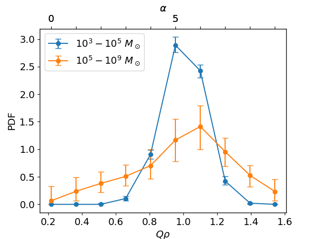
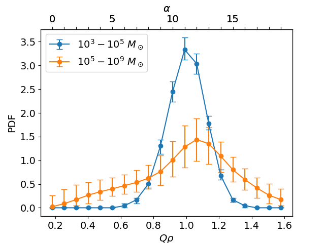
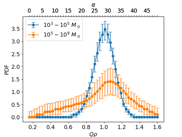
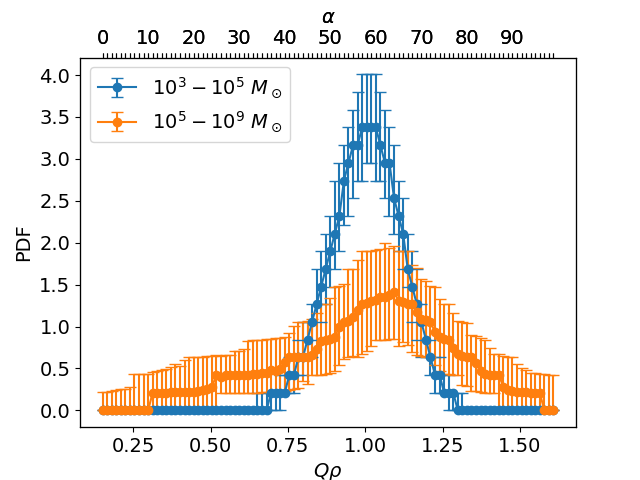
Figure 3: Interquantile ranges and medians for PDF bins of $Q\rho=\rho/\bar{\rho}$ profiles measured from simulations. Panels correspond to $N_{\rm bin}=10,20,50,100$ (top axes shows the bin number).

We compute histograms of simulated density profiles $Q\rho_{i}(l)=\rho_{i}(l)/\bar{\rho}_{i}(l)$ obtained sampling from Equation 1. Given the counts $c_{\alpha}$ for the $\alpha^{th}$ histogram bin of width $w_{\alpha}$, the respective density is obtained as $y_{\alpha}=\frac{c_{\alpha}}{w_{\alpha}\sum_{\beta}c_{\beta}}$, where the normalization is such that the integral of the distribution is equal to one. This determines the probability density function ${\rm PDF}(Q\rho)$. Figure 3 shows median values and interquantile ranges obtained computing the ${\rm PDF}(Q\rho)$ for all simulations and for different choices of the number of bins $N_{\rm bin}$. The range in $Q\rho$ is set to be the largest one where we have samples for both mass ranges. The ${\rm PDF}(Q\rho)$ functions are peaked around $Q\rho\approx 1$, but consistently with Figure 1 the larger mass ranges have broader profiles. The ${\rm PDF}(Q\rho)$ for the lower mass range is close to a normal distribution with mean $Q\rho=1$ and standard deviation $\sigma=\sigma_{\epsilon}=0.1$, consistently with the fact that it is strongly affected by shot noise $\epsilon$. Neglecting shot noise would enhance negative skewness.

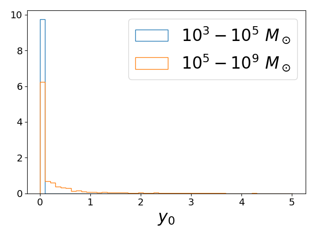
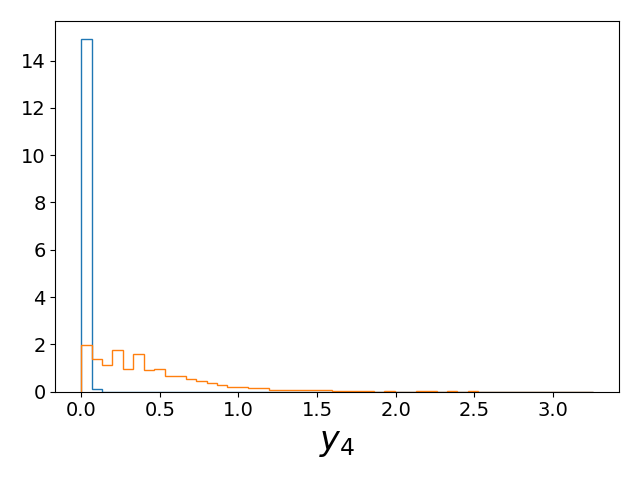
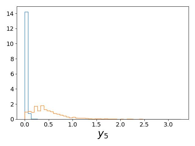
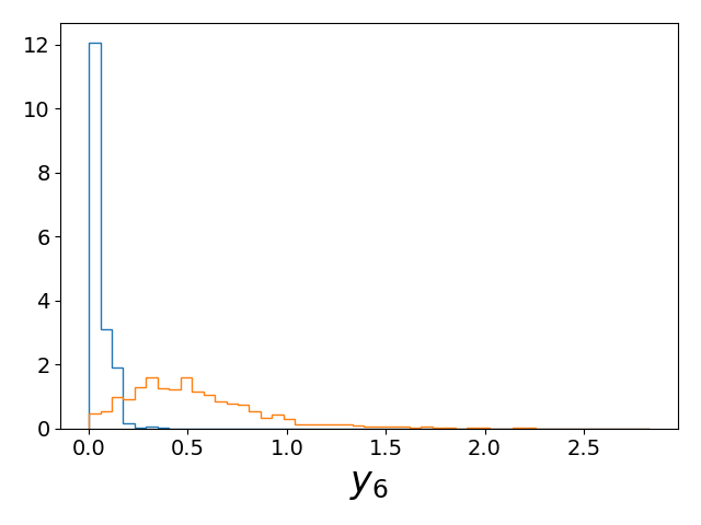
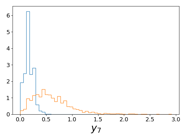
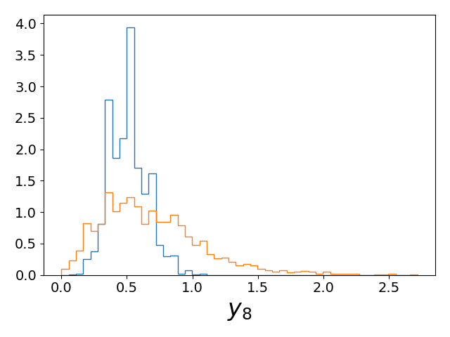
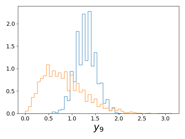
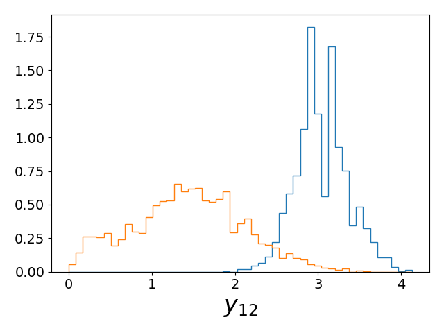
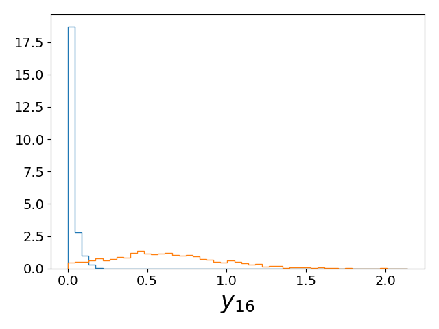
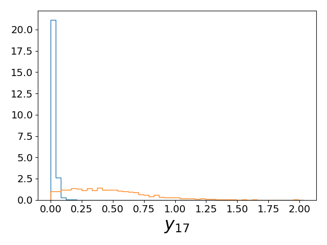
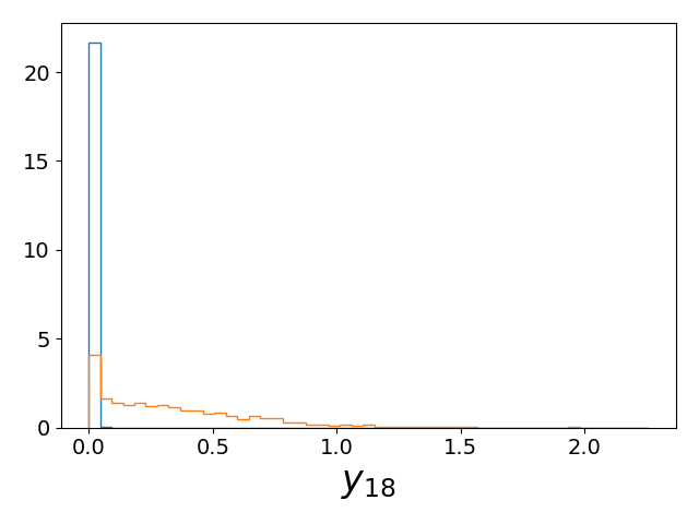
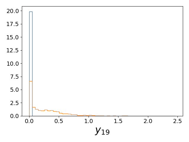
Figure 4: Panels show $y_{\alpha}$ distributions, namely the PDFs of each ${\rm PDF}(Q\rho)$ bin $\alpha$ for the $N_{\rm bin}=20$ case (see Figure 3 for comparison). Here we recover each $y_{\alpha}$ using 50 bins, but when performing model selection we marginalize over 10–500 bins. In panels corresponding to the tails of ${\rm PDF}(Q\rho)$ (i.e., small and large $\alpha$ values) we do not have enough resolution to estimate the PDF of the small mass case.

The PDF of each ${\rm PDF}(Q\rho)$ bin $y_{\alpha}$—i.e., ${\rm PDF}(y_{\alpha})$—provides an estimate of the probability distribution $\Pi(y_{\alpha}|\mathcal{M})$ for model $\mathcal{M}$. Our models $\mathcal{M}_{0}$ and $\mathcal{M}_{1}$ correspond to the $10^{3}$–$10^{5}M_{\Sun}$ and $10^{5}$–$10^{9}M_{\Sun}$ mass ranges, respectively. The $\Pi(y_{\alpha}|\mathcal{M})$ distributions so recovered based on simulations serves as prior for model selection. Figure 4 shows ${\rm PDF}(y_{\alpha})$ for all models. The small mass perturbers model is characterized by tiny $y_{\alpha}$ values for $\alpha$ bins corresponding to the tails of ${\rm PDF}(Q\rho)$ (see Figure 3), while all mass models show a log-normal distribution for $\alpha$ bins corresponding central regions of ${\rm PDF}(Q\rho)$.

3.1.2 Model selection

Let $p\left(\hat{y}_{\alpha}|y_{\alpha},\mathcal{M}\right)$ be the likelihood function for ${\rm PDF}(Q\rho)$ bin $\alpha$, where the hat denotes data. The Bayesian evidence for a given model $\mathcal{M}$ is given by:

$$E(\hat{y}_{\alpha}|\mathcal{M})=\int\ p(\hat{y}_{\alpha}|y_{\alpha},\mathcal{M})\Pi(y_{\alpha}|\mathcal{M})dy_{\alpha}\;,$$ (2)

where the prior $\Pi(y_{\alpha}|\mathcal{M})$ is computed based on simulations as outlined above. Then, model selection can rely on the Bayes factor:

$$B_{\alpha,ij}=\frac{E(\hat{y}_{\alpha}|\mathcal{M}_{i})}{E(\hat{y}_{\alpha}|\mathcal{M}_{j})}\;.$$ (3)

Since an analysis based on true data is beyond the scope of this work, here we rely again on simulations to estimate $p(\hat{y}_{\alpha}|y_{\alpha},\mathcal{M})$ in Equation 2 to forecast expected evidence values that will motivate further investigation based on true data. We consider different fiducial models:

$$p(\hat{y}_{\alpha}^{{\rm fid},i}|y_{\alpha})=\Pi(y_{\alpha}|\mathcal{M}_{i})\;,$$ (4)

for $i=0,1$. Note that we removed the dependence on the model on the left-hand side, as for each fiducial case $i$ we assume the likelihood to be the same; it is easy to relax this assumption if needed. Then we consider

$$E(\hat{y}_{\alpha}^{{\rm fid},i}|\mathcal{M}_{j})=\int_{0}^{\infty}p(\hat{y}_{\alpha}^{{\rm fid},i}|y_{\alpha})\Pi(y_{\alpha}|\mathcal{M}_{j})dy_{\alpha}\;,$$ (5)

where again $j=0,1,2$. This determines

$$B_{\alpha,ij}^{{\rm fid},i}=E(\hat{y}_{\alpha}^{{\rm fid},i}|\mathcal{M}_{i})/E(\hat{y}_{\alpha}^{{\rm fid},i}|\mathcal{M}_{j})\;,$$ (6)

which provides the strength of evidence for model $\mathcal{M}_{i}$ if the true underlying mass distribution is indeed consistent with $\mathcal{M}_{i}$.

We sample $\Pi(y_{\alpha}|\mathcal{M}_{i})$ using the same binning in $y_{\alpha}$ for all models $\mathcal{M}_{i}$ so that the product of the two distributions can be estimated by the product of the respective bin heights, and integrals are estimated using the trapezoidal rule. Methodological errors are estimated by marginalizing over the number of bins in $y_{\alpha}$.

3.2 Gradient Boosting classifier

We use the Python libraries Scikit-learn [41] and XGBoost [42] to train a gradient-boosted decision trees classifier. This model builds and ensemble of weak predictors (decision trees) to provide a robust predictor, optimizing an objective function with an iterative gradient descent algorithm. In our single-label (exclusive classes) binary classification case the objective is a logistic function, whose output is the probability of the $\mathcal{M}_{0}$ class [43].

Our data is composed by a vector $\boldsymbol{X}$ whose component $i$ is a given simulation sample $(Q\rho_{i}(l_{1}),Q\rho_{i}(l_{2}),\ldots,Q\rho_{i}(l_{n_{l}}))$, where $Q\rho_{i}(l)=\rho_{i}(l)/\bar{\rho}_{i}(l)$, and a vector $\boldsymbol{y}$ containing binary labels associated to the class corresponding to a given sample. We randomly split the density samples into testing (25% of the total samples), training and validation (75% and 25% of the remaining samples, respectively) sets. The training and validation samples are used to tune the model hyperparameters, while the testing sample is only used to evaluate the accuracy of the final model. Then, rather than considering all of the $n_{l}$ angular bins for each sample, we find it convenient to perform a Principal Component Analysis (PCA), and only keep $n_{\rm PCA}<n_{l}$ components. PCA is sensitive to the variance of the features $X_{i}$ that varies significantly in size. Hence, before computing the principal components we standardize the features by removing the mean and scaling to unit variance.

We then perform a 5-fold cross validation (CV) on the training set to optimize the maximum tree depth max_depth for base learners and the number of gradient boosted trees n_estimators. We find that optimizing the boosting learning rate does not affect substantially our results, due to its strong correlation with n_estimators. The search grid covers a few values for each hyperparameter (the full model has to be evaluated at each CV fold) within the max_depth $\in[2,128]$ and n_estimators $\in[10,200]$ ranges. The validation set is then used to evaluate the model pipeline based on the number of true positives $T_{p_{i}}$, true negatives $T_{n_{i}}$, false positives $F_{p_{i}}$ and false negatives $F_{n_{i}}$ for each class $\mathcal{M}_{i}$. As summary metrics we consider the accuracy

$$A_{i}=\frac{T_{p_{i}}+T_{n_{i}}}{T_{p_{i}}+T_{n_{i}}+F_{p_{i}}+F_{n_{i}}}\;,$$ (7)

precision

$$P_{i}=\frac{T_{p_{i}}}{T_{p_{i}}+F_{p_{i}}}\;,$$ (8)

recall

$$R_{i}=\frac{T_{p_{i}}}{T_{p_{i}}+F_{n_{i}}}\;,$$ (9)

and their harmonic average, or $F_{1}$-score

$$F_{1,i}=\frac{2}{1/P_{i}+1/R_{i}}\;.$$ (10)

We find that setting $n_{\rm PCA}=8$ explains 80% of the total variance and it is a reasonable compromise between good model performance and training speed. Setting a much lower or larger $n_{\rm PCA}$ (or not performing PCA) would worsen model performance by a few percentage points. While we expect that including more PCA components (or not performing PCA) should lead to at least comparable performance, this would require to run the CV search on a finer grid of hyperparameters. Furthermore, including more PCA components is up to 5 times more requiring in training speed.

4 Results

In this section we discuss results for both mass model selection methodologies outlined above.

4.1 Bayesian model selection based on PDF

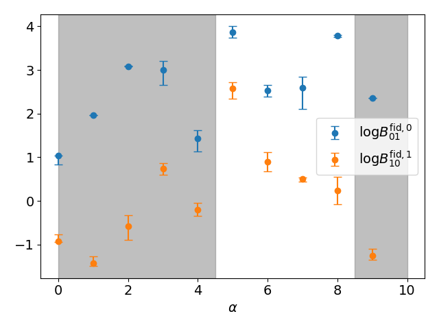
Figure 5: Bayes factors for different bins $\alpha$ of the PDF (see Figure 3) corresponding to $N_{\rm bin}=10,20,50,100$). Grey regions correspond to rare density fluctuations that are poorly sampled by our simulations, leading to unreliable evidence estimates.

Figure 5 shows evidence ratios defined in Equation 6 for different choices of the number $N_{\rm bin}$ of bins in $Q\rho$. For each ${\rm PDF}(Q\rho)$ bin $y_{\alpha}$ we compute the evidence ratio selecting different number of bins 10–500. Error bars correspond to interquantile ranges so obtained and their narrowness confirms that our evidence estimates based on the trapezoidal rule are robust against the binning in $y_{\alpha}$.

Results shown in Figure 5 are easily interpreted comparing with Figure 3 and Figure 4. Central $\alpha$ bins show the largest Bayes factor, as ${\rm PDF}(Q\rho)$ for the different models are significantly distinct. The crossing of ${\rm PDF}(Q\rho)$ curves in Figure 3 (see also $\alpha=8,13$ in Figure 4) leads to a decrease in $\log B$ as the models are less distinguishable, while it increases again towards the tails where the small mass model $\mathcal{M}_{0}$ has ${\rm PDF}(Q\rho)\approx 0$. $\log B$ eventually decreases for the outer bins as ${\rm PDF}(Q\rho)\to 0$ also for the larger mass model $\mathcal{M}_{1}$. Bins corresponding to the tails of ${\rm PDF}(Q\rho)$ distributions do not give reliable evidence estimates due to the poor resolution for small mass perturbers which leads to a single ${\rm PDF}(y_{\alpha})$ bin, see Figure 4. Hereon we neglect evidence for $\alpha$ bins outside the $\sim 3\sigma_{\epsilon}$ range from the peak of the low mass ${\rm PDF}(Q\rho)$ distribution, which is the most affected one by poor resolution. The excluded regions are shown as gray bands in Figure 5.

Table 1: Cumulative Bayes factor upper limits for different choices of the number of ${\rm PDF}(Q\rho)$ bins.

	10	20	50	100
$\sum\log B_{01}^{{\rm fid},0}$	9.0	18.0	33.1	53.5
$\sum\log B_{10}^{{\rm fid},1}$	4.0	5.4	3.1	1.3

The largest Bayes factors are in the range 2.5–4, depending on $N_{\rm bin}$, when the fiducial model is $\mathcal{M}_{0}$ (see $\log B_{01}^{{\rm fid},0}$). Bayes factors are smaller when the fiducial models is $\mathcal{M}_{1}$, as the corresponding ${\rm PDF}(Q\rho)$ profiles (see Figure 3 and Figure 4) are less sharp and characterized by larger dispersion. While a proper estimate of cumulative Bayes factors should include their correlation, an upper limit is given by summing $\log B_{\alpha}$ for all $\alpha$ indices (up to the excluded region commented above) as reported in Table 1. Assuming model $\mathcal{M}_{0}$ as fiducial leads to moderate or strong evidence. Assuming model $\mathcal{M}_{1}$ can instead lead to weak evidence. The largest evidences obtained when including more bins are expected to be more strongly suppressed by cross-bin evidence correlations that we neglect.

The analysis suggests that if CDM perturbers form clusters in the $10^{5}$–$10^{9}M_{\Sun}$ range it may be more difficult to exclude the $10^{3}$–$10^{5}M_{\Sun}$ hypothesis than the vice versa.

As an exercise to further explore the performance of the methodology, we repeated the computation considering three mass ranges instead of two, namely $10^{3}$–$10^{5}M_{\Sun}$, $10^{5}$–$10^{7}M_{\Sun}$ and $10^{7}$–$10^{9}M_{\Sun}$. Similarly to the case described above, we find that if CDM perturbers form clusters in the $10^{7}$–$10^{9}M_{\Sun}$ range it may be more difficult to exclude the $10^{3}$–$10^{5}M_{\Sun}$ or $10^{5}$–$10^{7}M_{\Sun}$ hypotheses than the vice versa, possibly leading to inconclusive results.

4.2 Gradient Boosting classifier

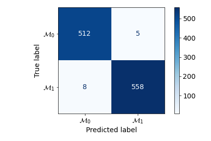
Figure 6: Confusion matrix obtained evaluating the gradient boosting model on the test dataset. Elements show the number of samples predicted to be associated to models $\mathcal{M}_{0}$ ($10^{3}$–$10^{5}M_{\Sun}$ CDM perturbers) and $\mathcal{M}_{1}$ ($10^{5}$–$10^{9}M_{\Sun}$) that are correctly (diagonal) or wrongly (non-diagonal) classified.

Table 2: Performance, relative to each mass category, of the gradient boosting classifier evaluated on the test set.

	Precision	Recall	$F_{1}$-score
$10^{3}$–$10^{5}M_{\Sun}$	0.98	0.99	0.99
$10^{5}$–$10^{9}M_{\Sun}$	0.99	0.99	0.99

Here we use the test set described in subsection 3.2 to evaluate the performance of the model trained on the training and validation sets. Given a $X_{i}$ sample from the test set, the model outputs the probabilities of it being associated with the $\mathcal{M}_{0}$ class. To compute the number of (in-)correctly classified elements we assign them to the $\mathcal{M}_{0}$ class if the respective probability is larger than 50%.

Figure 6 shows the confusion matrix reporting the number of correct classifications on the diagonal, and the number of wrong classifications on non-diagonal elements. Non-diagonal elements are much smaller than the diagonal ones. Compared to the PDF analysis, the gradient boosting algorithm shows strong discriminating power for all masses. This is confirmed by Table 2 showing the metrics described in Equation 8–Equation 10 evaluated on the test set. All classes are characterized by $98\%$–$99\%$ scores, and also accuracy (Equation 7) reaches $99\%$.

Also in this case we repeated the computation considering three mass ranges $10^{3}$–$10^{5}M_{\Sun}$, $10^{5}$–$10^{7}M_{\Sun}$ and $10^{7}$–$10^{9}M_{\Sun}$, confirming that the metrics described in Equation 8–Equation 10 give good results $\gtrsim 90\%$ for all classes, reaching 98% for the smaller mass one.

5 Conclusions

In our search for understanding one of the most elusive mysteries of nature, we have explored the information content associated with tidal stream collisions with dark matter clusters in the inner halo of our galaxy. We have introduced two complementary methodologies to constrain the mass of CDM perturbers on stellar streams and forecasted their potential ability based on GD-1-like stream simulations.

While the methodologies are independent from the dark matter model, we are interested in providing a simple test to discern specifically the PBH CDM hypothesis from the standard PDM one. If data favor stream perturbers in a small mass $10^{3}$–$10^{5}M_{\Sun}$ range over a larger one $10^{5}$–$10^{9}M_{\Sun}$ (within which PDM is typically analyzed) this will be a strong hint in favor of the PBH CDM hypothesis because a peak abundance of PBH clusters is expected in the smaller mass range.

As no simulation is available to date for neither PBH CDM nor PDM over $10^{3}$–$10^{5}M_{\Sun}$ mass scales, we modeled dark matter in this regime by extrapolating PDM results validated in the well known $10^{5}$–$10^{9}M_{\Sun}$ regime down to smaller masses. While this is conceptually in contrast with our simplifying hypothesis that mainly PBH CDM contributes to the $10^{3}$–$10^{5}M_{\Sun}$ range, forecasts are still useful to characterize the envisaged model selection capabilities and to justify further studies, especially considering that strong shot-noise mitigates this extrapolation errors.

The Bayesian PDF model selection provides a straightforward and robust analysis that, contrary to incomplete statistics such as the power spectrum, takes into account the fully non-Gaussian information of stellar streams density profiles. Including realistic observational errors, we expect large Bayes factors when taking the low mass ($10^{3}$–$10^{5}M_{\Sun}$, where a peak abundance of PBH CDM is expected) perturbers as the fiducial models. Instead, taking a large masses ($10^{5}$–$10^{9}M_{\Sun}$) model as the fiducial one may lead to inconclusive evidence, due to a larger dispersion in the PDF.

On the other hand, the gradient boosting model provides a complementary method to the PDF one that allows to classify an observed density profile according to the most likely mass range with high performance. While the PDF analysis relies on Bayesian model selection, this is not the case for the gradient boosting one; however, the path integral approach developed in [45] to compute Bayesian credible intervals for non-parametric genetic algorithms can also be adapted to our gradient boosting model. The excellent performance of the gradient boosting classifier also relies on the fact that the model takes into account the ordered information about the density profile dependence on the longitude, information that is instead lost in the PDF analysis. Figure 1 shows indeed an important dependence of perturbations on the angular distance from the progenitor, including a characteristic profile peaked towards the progenitor for large mass perturbers (which may bring to inconclusive evidence based on the PDF), differently from the low mass case. Another advantage of the gradient boosting algorithm is that it is a likelihood-free approach, contrary to the PDF analysis. While in this work we assumed different fiducial models for the latter, applying the PDF method to observations will require a detailed modeling of the likelihood.

To test of the robustness of the method and given theoretical uncertainties in the PBH modeling we verified that similar conclusions are reached when performing forecasts further dividing the largest mass range into $10^{5}$–$10^{7}M_{\Sun}$ and $10^{7}$–$10^{9}M_{\Sun}$ ranges, leading to a total of three mass ranges.

As an extension to the analysis presented here, we compared our gradient boosting classifier with a densely connected feedforward neural network classifier [43] with a few hidden layers composed by $\mathcal{O}(10)$ units, which gives comparable results only when neglecting shot noise and being significantly less performing for realistic observational errors. We also do not expected convolutional neural networks to bring substantial improvements because, due to their translational invariance, they would loose information about density perturbations as ordered sequences depending on longitude. Recurrent neural networks may be an interesting perspective that do not suffer from such a limitation, but due to typically high computational costs and the already good performance of our gradient boosting predictor, we don’t deem it as an urgent investigation. Another advantage of gradient boosting is that its hyperparameters are easily optimized, avoiding empirical iterations over different neural networks architectures.

We showed that stellar streams are a promising tool to investigate $10^{3}$–$10^{5}M_{\Sun}$ DM perturbers, a range outside the reach of other observations such as lensing and of interest to discriminate the PBH CDM hypothesis. As mentioned, our motivation of comparing this small subhalo objects mass range with the large ones $10^{5}$–$10^{9}M_{\Sun}$ to favor PBH CDM over particle DM relies on the simplified assumption that each model only contributes subhalo objects in the respective mass ranges. However, subhalo abundance is a continuous function spanning all the scales $10^{3}$–$10^{9}M_{\Sun}$ in the PDM scenario [16]. An important extension of our simplified picture is then to compare the PBH CDM against standard particle DM scenarios in the full $10^{3}$–$10^{9}M_{\Sun}$ range taking into account the respective perturbers abundance distributions. This will require N-body simulations down to $10^{3}M_{\Sun}$ scales for both DM models, not available to date (but see advances, e.g., from [7]). Note that by extrapolating particle DM results down to the unexplored $10^{3}$–$10^{5}M_{\Sun}$ mass range as done here underestimates the abundance of PBH CDM clusters, and a proper computation may increase the discriminating potential as a higher abundance of PBH objects over shot noise would sharpen the PDF distribution. Joint classification of other properties of the perturbers besides their mass, such as their size and concentration, is also valuable additional information to discriminate different DM models [15]. Besides density fluctuations investigated here, another relevant stream property in the line-of-parallel-angle approach is the track fluctuation [18].

Our methodologies can be readily applied to the GD-1 stream for which density perturbations data are already available [14, 23], complementing previous studies. It can also be extended to other streams, as long as the density profile along the stream is a good descriptor of the stellar dynamics, which is certainly the case for other relatively cold streams such as Palomar 5 [18]. Depending on the stream, perturbations induced by baryonic objects, subleading for our GD-1-like case, may be relevant and needed to be modeled accurately as they may induce similar effects as DM subhalo objects of large mass. Current observations from the GAIA and Dark Energy Survey (DES) missions are increasingly improving data about known streams and discovering new streams [46, 47], that will be further complemented with upcoming observations such as DESI [48] and the Rubin Observatory [49], which provide new promising ground for dark matter constraints.

Data Availability

The code underlying this article is available at https://gitlab.com/montanari/stream-dm.

Appendix A Convergence tests for small mass perturbers

In this section we repeat convergence tests explored in [18] to verify the reliability of numerical simulations for small masses perturbers $10^{3}$–$10^{5}M_{\Sun}$, and we study the effect of different perturber internal profiles. The range $10^{5}$–$10^{9}M_{\Sun}$ has already been extensively explored in [18], finding overall good convergence, except for the impact parameter factor $X$ at the largest scales. Following closely [18], to which we refer for further details, we compute power spectra of fluctuations in the density, $P_{Q\rho Q\rho}$, in the mean track in parallel frequency $\langle\Delta\Omega_{\parallel}\rangle$, $P_{\Omega\Omega}$, and their cross-spectrum, $P_{Q\rho\Omega}$. The power spectrum is computed Fourier-transforming the density profile normalized to the smooth one as a function of the parallel angle offset from the progenitor, $Q\rho(\Delta\theta_{\parallel})=\rho(\Delta\theta_{\parallel})/\bar{\rho}(\Delta\theta_{\parallel})$, which gives the dependence over the wave-number $k_{\theta}$. We proceed similarly for the mean track. For each case we compute at least $1000$ realizations to estimate the respective scatter, and show the simulations interquantile ranges as gray bands in the following figures.

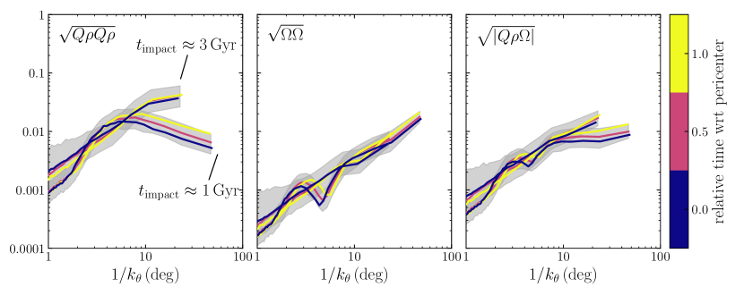
Figure 7: Power spectrum, as a function of the inverse Fourier mode, induced by $10^{3}$–$10^{5}\ M_{\odot}$ perturbers on a GD1-like stream if impacts happen at a single time, $\sim 1$ Gyr or $\sim 3$ Gyr. Different line colors correspond to a given orbital phase: pericenter, apocenter, or in between (the orbital period is $\sim 400$ Myr). Gray bands show the interquantile range for the set of simulations relative to a given case and solid curves show the median power spectrum.

First, we test the importance of the sampling of the orbital phase. As described in section 2, we sample impacts at discrete time values from the start of disruption to today. The sampling is chosen to be smaller than the orbital period, but it is independent of the orbital phase. To check whether this is a good strategy, we simulate the stream evolution assuming all of the impacts to happen at a single time, chosen to be close to the pericenter, apocenter or in between. We repeat this for two sets of time values $\sim 3$ Gyr and $\sim 1$ Gyr. Results are shown in figure 7. The two sets of impact times lead to significantly different spectra, which is expected given that impacts at $\sim 1$ Gyr have less time to evolve than impacts at $\sim 3$ Gyr, leading to less power. However, the dependence on the orbital phase is not statistically relevant for our purposes. [18] shows that considering larger perturber masses the relevance of the orbital phase is even smaller. Compared to [18] results, figure 7 shows smaller power (actually smaller than the shot noise level described in section 2) due to the smaller perturbers mass.

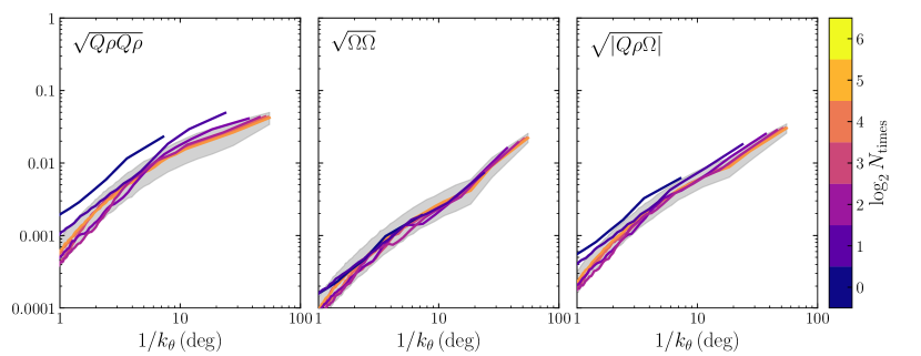
Figure 8: Power spectrum convergence for different values of the number of impact times since the start of the disruption of the stream. Results converge when the time interval between two impacts is comparable or smaller than the orbital period ($\sim 400$ Myr) of the $9$ Gyr-old stream.

Figure 8 shows the effect of different time samplings. Power spectra are already well converged considering only 16 impact times, corresponding to intervals of $\sim 560$ Myr. This suggests that a time sampling comparable to the orbital period of the stream ($\sim 400$ Myr) recovers well its statistical properties. In the convergence tests that follow, however, we consider 32 impact times (spaced by $\sim 280$ Myr) so that the time interval between two impacts is smaller than the orbital period. Furthermore, in the main analysis we set an even more conservative choice (although more computationally requiring) of 64 impact times, corresponding to intervals of $\sim 140$ Myr. The larger mass range shows similar good convergence [18].

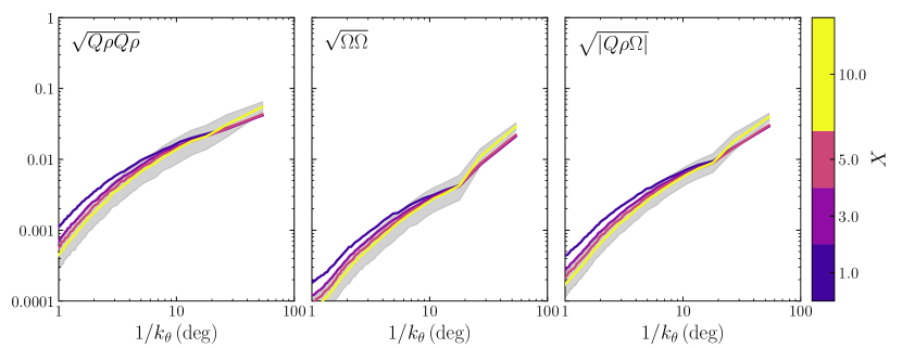
Figure 9: Power spectrum convergence for different values of the impact parameter factor $X$. (Note that the larger mass range $10^{5}$–$10^{9}M_{\Sun}$, not shown here, do not fully converge at the largest scales.)

Figure 9 shows the effect of different impact parameter factors $X$. Small scales converge for $X\gtrsim 3$ and (our fiducial value in the main analysis and in other convergence tests is $X=5$). However, note that the larger mass range $10^{5}$–$10^{9}M_{\Sun}$ do not fully converge at the largest scales ($\gtrsim 30^{\circ}$) as the impulse approximation is no longer reliable and distant encounters are important [18].

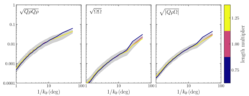
Figure 10: Power spectrum convergence for different values of the length scale, relative to the fiducial stream length, within which impacts are sampled.

Figure 10 shows the effect of different length factors determining up to what distance from the progenitor impacts are sampled. The length scale coincide with the stream length, whose edge is defined as the location along the stream where the density drops by 20% compared to the respective value close to the progenitor. Setting different length multipliers to sample impacts up to 75% and 125% of the fiducial length shows good convergence (to keep the same number of impacts for all the cases we also scale the predicted density of perturbers together with the length factor). The larger mass range shows similar good convergence [18].

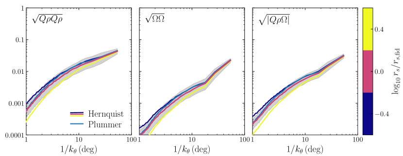
Figure 11: Power spectrum for different scaling of the fiducial Hernquist scale parameter $r_{s}(M)$, and for a plummer profile.

Figure 11 compares different perturber profiles. The fiducial Hernquist profile scale is set by $r_{s,{\rm fid}}(M)=1.05{\rm kpc}\ (M/10^{8}M_{\odot})^{0.5}$, obtained by fitting the Via Lactea II simulation [18, 38]. We first investigate a constant factor scaling 2.5 times larger or smaller than the fiducial relation (for consistency with the maximum sampled value of the impact parameter, we also set an impact parameter factor $X$ such that $X=X_{\rm fid}r_{s,{\rm fid}}/r_{s}$, where $X_{\rm fid}=5$), which roughly corresponds to the scatter observed in the Via Lactea II simulation. Then we also compare the power spectrum obtained assuming a Plummer profile $r_{s}(M)=1.62{\rm kpc}\ (M/10^{8}M_{\odot})^{0.5}$ (also here for consistency we need to set an impact parameter factor $X$ such that $X=(1.05/1.62)X_{fid}$, where we take the ratio of the constant factors appearing in the Hernquist and Plummer scale parameters). Although more compact perturbers induce larger power on the smallest scales, differences are negligible for our purposes, as is the case for the larger mass range [18]. Deviations are particularly small when comparing Hernquist and Plummer profiles, the main difference being the inner region of the perturber (cuspy for the first case, and smoothed in the second one) that is not relevant for our purposes.

Appendix B Power spectrum dependence on mass range

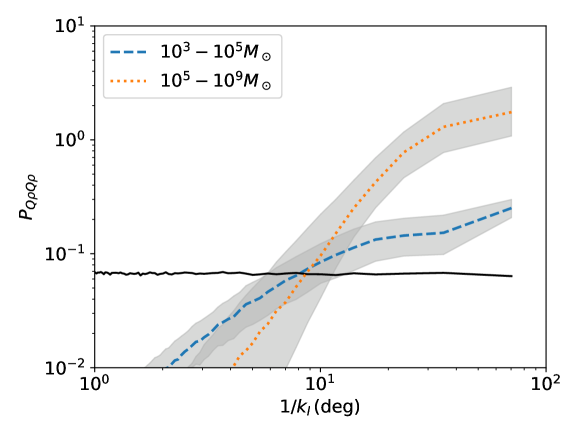
Figure 12: Power spectrum of density fluctuations $Q\rho$ for the mass ranges considered in the main analysis. Gray bands show the interquantile range. The solid line shows the shot noise contribution.

In this section we show the power spectrum of density fluctuations $Q\rho$ for both mass ranges considered in the main analysis. The computation and interpretation of the power spectrum proceeds similarly to A, but we Fourier-transform the density as a function of the observable Galactic longitude $Q\rho(l)$, which gives the dependence over the wave-number $k_{l}$. This allows us to include the contribution of shot noise (see section 2) as the median of $10^{3}$ realizations of Gaussian noise.

Both cases are detectable above shot noise over $1/k_{l}>8$ deg scales and they are clearly distinguishable at the largest scales, over $1/k_{l}>20$ deg. While it would be interesting to compare model selection performance based on these power spectra to the methods outlined in the main analysis, a proper estimate of the Bayesian evidence is computationally prohibitive for the power spectrum. Note that our PDF methodology provides robust results for the Bayes factors relying on only $\mathcal{O}(10^{3})$ simulations thanks to the fact that we disregard bins where the evidence computation is not reliable due to poor sampling, see subsection 4.1. While the power spectrum has the advantage over the PDF of retaining spatial information, density fluctuations are highly non-Gaussian so the power spectrum is an incomplete summary statistics and the infinite series of higher correlation moments is expected to contain valuable complementary information. Neither of the gradient boosting nor the PDF method proposed in the main analysis suffer from this limitation.

References

- [1] J. García-Bellido, Massive Primordial Black Holes as Dark Matter and their detection with Gravitational Waves, J. Phys. Conf. Ser. 840 (1) (2017) 012032 (2017). arXiv:1702.08275, doi:10.1088/1742-6596/840/1/012032.
- [2] B. P. Abbott, et al., GW151226: Observation of Gravitational Waves from a 22-Solar-Mass Binary Black Hole Coalescence, Phys. Rev. Lett. 116 (24) (2016) 241103 (2016). arXiv:1606.04855, doi:10.1103/PhysRevLett.116.241103.
- [3] J. García-Bellido, A. D. Linde, D. Wands, Density perturbations and black hole formation in hybrid inflation, Phys. Rev. D54 (1996) 6040–6058 (1996). arXiv:astro-ph/9605094, doi:10.1103/PhysRevD.54.6040.
- [4] J. M. Ezquiaga, J. García-Bellido, V. Vennin, The exponential tail of inflationary fluctuations: consequences for primordial black holes, JCAP 2003 (2020) 029 (2020). arXiv:1912.05399, doi:10.1088/1475-7516/2020/03/029.
- [5] S. Clesse, J. García-Bellido, Seven Hints for Primordial Black Hole Dark Matter, Phys. Dark Univ. 22 (2018) 137–146 (2018). arXiv:1711.10458, doi:10.1016/j.dark.2018.08.004.
- [6] B. Carr, S. Clesse, J. García-Bellido, F. Kuhnel, Cosmic Conundra Explained by Thermal History and Primordial Black Holes, Phys. Dark Univ. 31 (2021) 100755 (2021). arXiv:1906.08217, doi:10.1016/j.dark.2020.100755.
- [7] M. Trashorras, J. García-Bellido, S. Nesseris, The clustering dynamics of primordial black boles in -body simulations, Universe 7 (1) (2021) 18 (2021). arXiv:2006.15018, doi:10.3390/universe7010018.
- [8] J. Zavala, C. S. Frenk, Dark matter haloes and subhaloes, Galaxies 7 (4) (2019) 81 (2019). arXiv:1907.11775, doi:10.3390/galaxies7040081.
- [9] F. Montanari, D. Barrado, J. García-Bellido, Searching for correlations in GAIA DR2 unbound star trajectories, Mon. Not. Roy. Astron. Soc. 490 (4) (2019) 5647–5657 (2019). arXiv:1907.09298, doi:10.1093/mnras/stz2959.
- [10] A. J. Allen, D. O. Richstone, Tidal Limitation of Stellar Systems on Both Circular and Elongated Orbits, ApJ 325 (1988) 583 (Feb. 1988). doi:10.1086/166029.
- [11] B. Moore, M. Davis, The origin of the Magellanic Stream., MNRAS 270 (1994) 209–221 (Sep. 1994). arXiv:astro-ph/9401008, doi:10.1093/mnras/270.2.209.
- [12] K. V. Johnston, D. N. Spergel, L. Hernquist, The Disruption of the Sagittarius Dwarf Galaxy, ApJ 451 (1995) 598 (Oct. 1995). arXiv:astro-ph/9502005, doi:10.1086/176247.
- [13] R. A. Ibata, G. F. Lewis, M. J. Irwin, Uncovering cdm halo substructure with tidal streams, Mon. Not. Roy. Astron. Soc. 332 (2002) 915 (2002). arXiv:astro-ph/0110690, doi:10.1046/j.1365-8711.2002.05358.x.
- [14] N. Banik, J. Bovy, G. Bertone, D. Erkal, T. de Boer, Evidence of a population of dark subhalos from Gaia and Pan-STARRS observations of the GD-1 stream (11 2019). arXiv:1911.02662.
- [15] A. Bonaca, D. W. Hogg, A. M. Price-Whelan, C. Conroy, The Spur and the Gap in GD-1: Dynamical Evidence for a Dark Substructure in the Milky Way Halo, ApJ 880 (1) (2019) 38 (Jul. 2019). arXiv:1811.03631, doi:10.3847/1538-4357/ab2873.
- [16] E. Bertschinger, The Effects of Cold Dark Matter Decoupling and Pair Annihilation on Cosmological Perturbations, Phys. Rev. D 74 (2006) 063509 (2006). arXiv:astro-ph/0607319, doi:10.1103/PhysRevD.74.063509.
- [17] M. Petac, Hunt for dark subhalos in the galactic stellar field using computer vision, arXiv e-prints (2019) arXiv:1910.02492 (Oct. 2019). arXiv:1910.02492.
- [18] J. Bovy, D. Erkal, J. L. Sanders, Linear perturbation theory for tidal streams and the small-scale CDM power spectrum, Mon. Not. Roy. Astron. Soc. 466 (1) (2017) 628–668 (2017). arXiv:1606.03470, doi:10.1093/mnras/stw3067.
- [19] N. Banik, G. Bertone, J. Bovy, N. Bozorgnia, Probing the nature of dark matter particles with stellar streams, JCAP 1807 (2018) 061 (2018). arXiv:1804.04384, doi:10.1088/1475-7516/2018/07/061.
- [20] N. Banik, J. Bovy, Effects of baryonic and dark matter substructure on the Pal 5 stream, Mon. Not. Roy. Astron. Soc. 484 (2) (2019) 2009–2020 (2019). arXiv:1809.09640, doi:10.1093/mnras/stz142.
- [21] N. Banik, J. Bovy, G. Bertone, D. Erkal, T. J. L. de Boer, Novel constraints on the particle nature of dark matter from stellar streams, arXiv e-prints (2019) arXiv:1911.02663 (Nov. 2019). arXiv:1911.02663.
- [22] N. Dalal, J. Bovy, L. Hui, X. Li, Don’t cross the streams: caustics from Fuzzy Dark Matter (11 2020). arXiv:2011.13141.
- [23] J. Hermans, N. Banik, C. Weniger, G. Bertone, G. Louppe, Towards constraining warm dark matter with stellar streams through neural simulation-based inference (11 2020). arXiv:2011.14923.
- [24] A. Bonaca, C. Conroy, D. W. Hogg, P. A. Cargile, N. Caldwell, R. P. Naidu, A. M. Price-Whelan, J. S. Speagle, B. D. Johnson, High-resolution Spectroscopy of the GD-1 Stellar Stream Localizes the Perturber near the Orbital Plane of Sagittarius, ApJ 892 (2) (2020) L37 (Apr. 2020). arXiv:2001.07215, doi:10.3847/2041-8213/ab800c.
- [25] M. T. Gialluca, R. P. Naidu, A. Bonaca, Velocity Dispersion of the GD-1 Stellar Stream (11 2020). arXiv:2011.12963.
- [26] K. Malhan, M. Valluri, K. Freese, Probing the nature of dark matter with accreted globular cluster streams, MNRAS 501 (1) (2021) 179–200 (Jan. 2021). arXiv:2005.12919, doi:10.1093/mnras/staa3597.
- [27] D. Erkal, V. Belokurov, J. Bovy, J. L. Sand ers, The number and size of subhalo-induced gaps in stellar streams, MNRAS 463 (1) (2016) 102–119 (Nov. 2016). arXiv:1606.04946, doi:10.1093/mnras/stw1957.
- [28] K. Patton, J. Blazek, K. Honscheid, E. Huff, P. Melchior, A. J. Ross, E. Suchyta, Cosmological constraints from the convergence 1-point probability distribution, Mon. Not. Roy. Astron. Soc. 472 (1) (2017) 439–446 (2017). arXiv:1611.01486, doi:10.1093/mnras/stx1626.
- [29] D. Gruen, et al., Density Split Statistics: Cosmological Constraints from Counts and Lensing in Cells in DES Y1 and SDSS Data, Phys. Rev. D 98 (2) (2018) 023507 (2018). arXiv:1710.05045, doi:10.1103/PhysRevD.98.023507.
- [30] A. I. Salvador, et al., Measuring Linear and Non-linear Galaxy Bias Using Counts-in-Cells in the Dark Energy Survey Science Verification Data, Mon. Not. Roy. Astron. Soc. 482 (2) (2019) 1435–1451 (2019). arXiv:1807.10331, doi:10.1093/mnras/sty2802.
- [31] C. Uhlemann, O. Friedrich, F. Villaescusa-Navarro, A. Banerjee, S. Codis, Fisher for complements: Extracting cosmology and neutrino mass from the counts-in-cells PDF, Mon. Not. Roy. Astron. Soc. 495 (4) (2020) 4006–4027 (2020). arXiv:1911.11158, doi:10.1093/mnras/staa1155.
- [32] D. Zürcher, J. Fluri, R. Sgier, T. Kacprzak, A. Refregier, Cosmological Forecast for non-Gaussian Statistics in large-scale weak Lensing Surveys, JCAP 01 (2021) 028 (2021). arXiv:2006.12506, doi:10.1088/1475-7516/2021/01/028.
- [33] J. Bovy, Dynamical modeling of tidal streams, Astrophys. J. 795 (1) (2014) 95 (2014). arXiv:1401.2985, doi:10.1088/0004-637X/795/1/95.
- [34] J. L. Sanders, J. Bovy, D. Erkal, Dynamics of stream-subhalo interactions, MNRAS 457 (4) (2016) 3817–3835 (Apr. 2016). arXiv:1510.03426, doi:10.1093/mnras/stw232.
- [35] J. Bovy, galpy: A Python Library for Galactic Dynamics, Astrophys. J. Suppl. 216 (2) (2015) 29 (2015). arXiv:1412.3451, doi:10.1088/0067-0049/216/2/29.
- [36] J. J. Webb, J. Bovy, Searching for the GD-1 stream progenitor in Gaia DR2 with direct N-body simulations, MNRAS 485 (4) (2019) 5929–5938 (Jun. 2019). arXiv:1811.07022, doi:10.1093/mnras/stz867.
- [37] J. H. Yoon, K. V. Johnston, D. W. Hogg, Clumpy Streams from Clumpy Halos: Detecting Missing Satellites with Cold Stellar Structures, ApJ 731 (1) (2011) 58 (Apr. 2011). arXiv:1012.2884, doi:10.1088/0004-637X/731/1/58.
- [38] J. Diemand, M. Kuhlen, P. Madau, M. Zemp, B. Moore, D. Potter, J. Stadel, Clumps and streams in the local dark matter distribution, Nature 454 (7205) (2008) 735–738 (Aug. 2008). arXiv:0805.1244, doi:10.1038/nature07153.
- [39] P. Henrici, Elements of numerical analysis, Wiley, New York, 1964 (1964).
- [40] R. Trotta, Bayesian Methods in Cosmology, 2017 (1 2017). arXiv:1701.01467.
- [41] F. Pedregosa, G. Varoquaux, A. Gramfort, V. Michel, B. Thirion, O. Grisel, M. Blondel, P. Prettenhofer, R. Weiss, V. Dubourg, J. Vanderplas, A. Passos, D. Cournapeau, M. Brucher, M. Perrot, E. Duchesnay, Scikit-learn: Machine learning in Python, Journal of Machine Learning Research 12 (2011) 2825–2830 (2011).
-
[42]
T. Chen, C. Guestrin,
XGBoost: A scalable tree
boosting system, in: Proceedings of the 22nd ACM SIGKDD International
Conference on Knowledge Discovery and Data Mining, KDD ’16, ACM, New York,
NY, USA, 2016, pp. 785–794 (2016).
doi:10.1145/2939672.2939785.
URL http://doi.acm.org/10.1145/2939672.2939785 - [43] I. Goodfellow, Y. Bengio, A. Courville, Deep Learning, The MIT Press, 2016 (2016).
- [44] S. Nesseris, J. García-Bellido, Is the Jeffreys’ scale a reliable tool for Bayesian model comparison in cosmology?, JCAP 08 (2013) 036 (2013). arXiv:1210.7652, doi:10.1088/1475-7516/2013/08/036.
- [45] S. Nesseris, J. García-Bellido, Comparative analysis of model-independent methods for exploring the nature of dark energy, Phys. Rev. D 88 (6) (2013) 063521 (2013). arXiv:1306.4885, doi:10.1103/PhysRevD.88.063521.
- [46] T. S. Li, S. E. Koposov, D. B. Zucker, G. F. Lewis, K. Kuehn, J. D. Simpson, A. P. Ji, N. Shipp, Y. Y. Mao, M. Geha, A. B. Pace, A. D. Mackey, S. Allam, D. L. Tucker, G. S. Da Costa, D. Erkal, J. D. Simon, J. R. Mould, S. L. Martell, Z. Wan, G. M. De Silva, K. Bechtol, E. Balbinot, V. Belokurov, J. Bland-Hawthorn, A. R. Casey, L. Cullinane, A. Drlica-Wagner, S. Sharma, A. K. Vivas, R. H. Wechsler, B. Yanny, S5 Collaboration, The southern stellar stream spectroscopic survey (S5): Overview, target selection, data reduction, validation, and early science, MNRAS 490 (3) (2019) 3508–3531 (Dec. 2019). arXiv:1907.09481, doi:10.1093/mnras/stz2731.
- [47] R. Ibata, K. Malhan, N. Martin, D. Aubert, B. Famaey, P. Bianchini, G. Monari, A. Siebert, G. F. Thomas, M. Bellazzini, P. Bonifacio, E. Caffau, F. Renaud, Charting the Galactic acceleration field I. A search for stellar streams with Gaia DR2 and EDR3 with follow-up from ESPaDOnS and UVES, arXiv e-prints (2020) arXiv:2012.05245 (Dec. 2020). arXiv:2012.05245.
- [48] DESI Collaboration, A. Aghamousa, J. Aguilar, S. Ahlen, S. Alam, L. E. Allen, C. Allende Prieto, J. Annis, S. Bailey, C. Balland, O. Ballester, C. Baltay, L. Beaufore, C. Bebek, T. C. Beers, E. F. Bell, J. L. Bernal, R. Besuner, F. Beutler, C. Blake, H. Bleuler, M. Blomqvist, R. Blum, A. S. Bolton, C. Briceno, D. Brooks, J. R. Brownstein, E. Buckley-Geer, A. Burden, E. Burtin, N. G. Busca, R. N. Cahn, Y.-C. Cai, L. Cardiel-Sas, R. G. Carlberg, P.-H. Carton, R. Casas, F. J. Castander, J. L. Cervantes-Cota, T. M. Claybaugh, M. Close, C. T. Coker, S. Cole, J. Comparat, A. P. Cooper, M. C. Cousinou, M. Crocce, J.-G. Cuby, D. P. Cunningham, T. M. Davis, K. S. Dawson, A. de la Macorra, J. De Vicente, T. Delubac, M. Derwent, A. Dey, G. Dhungana, Z. Ding, P. Doel, Y. T. Duan, A. Ealet, J. Edelstein, S. Eftekharzadeh, D. J. Eisenstein, A. Elliott, S. Escoffier, M. Evatt, P. Fagrelius, X. Fan, K. Fanning, A. Farahi, J. Farihi, G. Favole, Y. Feng, E. Fernandez, J. R. Findlay, D. P. Finkbeiner, M. J. Fitzpatrick, B. Flaugher, S. Flender, A. Font-Ribera, J. E. Forero-Romero, P. Fosalba, C. S. Frenk, M. Fumagalli, B. T. Gaensicke, G. Gallo, J. Garcia-Bellido, E. Gaztanaga, N. Pietro Gentile Fusillo, T. Gerard, I. Gershkovich, T. Giannantonio, D. Gillet, G. Gonzalez-de-Rivera, V. Gonzalez-Perez, S. Gott, O. Graur, G. Gutierrez, J. Guy, S. Habib, H. Heetderks, I. Heetderks, K. Heitmann, W. A. Hellwing, D. A. Herrera, S. Ho, S. Holland, K. Honscheid, E. Huff, T. A. Hutchinson, D. Huterer, H. S. Hwang, J. M. Illa Laguna, Y. Ishikawa, D. Jacobs, N. Jeffrey, P. Jelinsky, E. Jennings, L. Jiang, J. Jimenez, J. Johnson, R. Joyce, E. Jullo, S. Juneau, S. Kama, A. Karcher, S. Karkar, R. Kehoe, N. Kennamer, S. Kent, M. Kilbinger, A. G. Kim, D. Kirkby, T. Kisner, E. Kitanidis, J.-P. Kneib, S. Koposov, E. Kovacs, K. Koyama, A. Kremin, R. Kron, L. Kronig, A. Kueter-Young, C. G. Lacey, R. Lafever, O. Lahav, A. Lambert, M. Lampton, M. Landriau, D. Lang, T. R. Lauer, J.-M. Le Goff, L. Le Guillou, A. Le Van Suu, J. H. Lee, S.-J. Lee, D. Leitner, M. Lesser, M. E. Levi, B. L’Huillier, B. Li, M. Liang, H. Lin, E. Linder, S. R. Loebman, Z. Lukić, J. Ma, N. MacCrann, C. Magneville, L. Makarem, M. Manera, C. J. Manser, R. Marshall, P. Martini, R. Massey, T. Matheson, J. McCauley, P. McDonald, I. D. McGreer, A. Meisner, N. Metcalfe, T. N. Miller, R. Miquel, J. Moustakas, A. Myers, M. Naik, J. A. Newman, R. C. Nichol, A. Nicola, L. Nicolati da Costa, J. Nie, G. Niz, P. Norberg, B. Nord, D. Norman, P. Nugent, T. O’Brien, M. Oh, K. A. G. Olsen, C. Padilla, H. Padmanabhan, N. Padmanabhan, N. Palanque-Delabrouille, A. Palmese, D. Pappalardo, I. Pâris, C. Park, A. Patej, J. A. Peacock, H. V. Peiris, X. Peng, W. J. Percival, S. Perruchot, M. M. Pieri, R. Pogge, J. E. Pollack, C. Poppett, F. Prada, A. Prakash, R. G. Probst, D. Rabinowitz, A. Raichoor, C. H. Ree, A. Refregier, X. Regal, B. Reid, K. Reil, M. Rezaie, C. M. Rockosi, N. Roe, S. Ronayette, A. Roodman, A. J. Ross, N. P. Ross, G. Rossi, E. Rozo, V. Ruhlmann-Kleider, E. S. Rykoff, C. Sabiu, L. Samushia, E. Sanchez, J. Sanchez, D. J. Schlegel, M. Schneider, M. Schubnell, A. Secroun, U. Seljak, H.-J. Seo, S. Serrano, A. Shafieloo, H. Shan, R. Sharples, M. J. Sholl, W. V. Shourt, J. H. Silber, D. R. Silva, M. M. Sirk, A. Slosar, A. Smith, G. F. Smoot, D. Som, Y.-S. Song, D. Sprayberry, R. Staten, A. Stefanik, G. Tarle, S. Sien Tie, J. L. Tinker, R. Tojeiro, F. Valdes, O. Valenzuela, M. Valluri, M. Vargas-Magana, L. Verde, A. R. Walker, J. Wang, Y. Wang, B. A. Weaver, C. Weaverdyck, R. H. Wechsler, D. H. Weinberg, M. White, Q. Yang, C. Yeche, T. Zhang, G.-B. Zhao, Y. Zheng, X. Zhou, Z. Zhou, Y. Zhu, H. Zou, Y. Zu, The DESI Experiment Part I: Science,Targeting, and Survey Design, arXiv e-prints (2016) arXiv:1611.00036 (Oct. 2016). arXiv:1611.00036.
- [49] v. Ivezić, et al., LSST: from Science Drivers to Reference Design and Anticipated Data Products, Astrophys. J. 873 (2) (2019) 111 (2019). arXiv:0805.2366, doi:10.3847/1538-4357/ab042c.