A critical review of LASSO and its derivatives for variable selection under dependence among covariates

Abstract

We study the limitations of the well known LASSO regression as a variable selector when there exists dependence structures among covariates. We analyze both the classic situation with $n\geq p$ and the high dimensional framework with $p>n$. Restrictive properties of this methodology to guarantee optimality, as well as the inconveniences in practice, are analyzed. Examples of these drawbacks are showed by means of a extensive simulation study, making use of different dependence scenarios. In order to search for improvements, a broad comparison with LASSO derivatives and alternatives is carried out. Eventually, we give some guidance about what procedures are the best in terms of the data nature.

Key words— Covariates selection; $p>n$; $L_{1}$ regularization techniques; LASSO.

1 Introduction and motivation

Nowadays, in many important statistical applications, it is of high relevance to apply a first variable selection step to correctly explain the data and avoid unnecessary noise. Furthermore, it is usual to find that the number of variables $p$ is larger than the number of available samples $n$ ($p>n$). Some examples of fields where this framework arises are processing image, statistical signal processing, genomics or functional magnetic resonance imaging (fMRI) among others. It is in the $p>n$ context where the ordinary models fail and, as a result, estimation and prediction in these settings are generally acknowledged as an important challenge in contemporary statistics.

In this framework, one of the most studied fields is the regression models adjustment. The idea of a regression model is to explain a variable of interest, $Y$, using $p$ covariates $X_{1},\dots,X_{p}$. This is done by means of a structure $m(X)$, $X=(X_{1},\dots,X_{p})^{\top}\in\mathbb{R}^{p}$, and an unknown error $\varepsilon$:

$$Y=m(X)+\varepsilon.$$ (1)

Here, $m(X)$ denotes the type of relation between the dependent variable $Y$ and the $p$ explanatory covariates, while $\varepsilon$ is the term which captures the remaining information as well as other unobserved fluctuations. This is typically assumed to have null mean and variance $\sigma^{2}$.

Once the $m(X)$ structure of (1) is estimated, it is possible to know the importance of every $X_{1},\dots,X_{p}$ in terms of explaining $Y$ apart from making predictions. Nevertheless, this estimation when $p>n$ still is a difficult and open problem in many situations. In particular, its easiest expression: the linear regression model, has been widely studied in the last years so as to provide efficient algorithms to fit this (see for example giraud2014introduction or hastie2015statistical).

In linear regression, as the name suggests, the relationship between $Y$ and $X$ is assumed to be linear, giving place to the model:

$$Y=X\beta+\varepsilon,$$ (2)

where $\beta\in\mathbb{R}^{p}$ is a coefficients vector to estimate. Note that we assume the covariates $X_{1},\dots,X_{p}$ and the response $Y$ centered, excluding the intercept from the model without loss of generality.

Having data $(y_{i},\mathbf{x_{i}})\in\mathbb{R}^{p+1}$ for $i=1,\dots,n$ samples, denoting $y=(y_{1},\dots,y_{n})^{\top}\in\mathbb{R}^{n}$ and $\mathbf{X}=(\mathbf{x_{1}},\dots,\mathbf{x_{p}})\in\mathbb{R}^{n\times p}$ with $\mathbf{x_{j}}=(x_{ij})_{i=1}^{n}\in\mathbb{R}^{n}$ for $j=1,\dots,p$, the $\beta$ vector can be estimated using the classical ordinary least squares (OLS) method solving (3).

$$\hat{\beta}^{OLS}=\min_{\beta}\left\{\sum_{i=1}^{n}\left(y_{i}-\sum_{j=1}^{p}x_{ij}\beta_{j}\right)^{2}\right\}$$ (3)

This estimator, $\hat{\beta}^{OLS}=(\mathbf{X}^{\top}\mathbf{X})^{-1}\mathbf{X}^{\top}y$, enjoys some desirable properties such as being an unbiased and consistent $\beta$ estimator of minimum variance.

Nevertheless, when $p>n$, this estimation method fails, as there are infinite solutions for the problem (3). Then, it is necessary to impose modifications on the procedure or to consider new estimation algorithms able to recover the $\beta$ values.

In order to overcome this drawback, the LASSO regression (Tibshirani1996) is still widely used due to its capability of reducing the dimension of the problem. This methodology assumes sparsity in the coefficient vector $\beta$, resulting in an easier interpretation of the model and performing variable selection. However, some rigid assumptions on the covariates matrix and sample size are needed so as to guarantee its good behavior (see, for example, Meinshausen2010). Moreover, the LASSO procedure exhibits some drawbacks related to the correct selection of covariates and the exclusion of redundant information (see Su2017), aside from bias. This can be easily showed in controlled simulated scenarios where it is known that only a small part of the covariates are relevant.

Hence, is this always the best option or at least a good start point? We have not found a totally convincing answer to this question in the literature. So as to test its performance and extract some general conclusions, the characteristics of the LASSO procedure are analyzed in this article. For this purpose, we start revisiting the existing literature about this topic as well as its most important adaptations. Furthermore, in view of the LASSO limitations, a global comparison is developed so as to test which procedures are capable of overcoming these in different dependence contexts, comparing their performance with alternatives which have proved their efficiency. Finally, some broad conclusions are drawn.

The article is organized as follows, in Section 2 a complete overview of the LASSO regression is given, including a summary of the requirements and inconveniences this algorithm has to deal with. In Section 3, some special simulation scenarios are introduced and used to illustrate the problems of this methodology in practice, testing the behavior of the LASSO under different dependence structures. In Section 4 the evolution of the LASSO in the last years is analyzed. Besides, other efficient alternatives in covariates selection are briefly described and their performance is compared with the LASSO one. Eventually, in Section LABEL:conclusions, a discussion is carried out so as to give some guidance about what types of covariates selection procedures are the best ones in terms of the data dependence structure.

2 A complete overview of the LASSO regression

In a linear regression model as the one of (2), there are a lot of situations where not all $p$ explanatory covariates are relevant, but several are unnecessary. In these scenarios we can assume that the $\beta$ vector is sparse and then search for the important covariates, avoiding noisy ones. The idea is, somehow, to obtain a methodology able to compare the covariates and select only those most important, discarding irrelevant information and keeping the error of prediction as small as possible. As there are $2^{p}$ possible sub-models, it tends to be rather costly to compare all of them using techniques such as forward selection or backward elimination.

One of the most typical solutions is to impose a restriction on the number of included covariates. This is done by means of adding some constraints to the OLS problem (3).

This brings up the idea of a model selection criterion, which express a trade-off between the goodness of fit and the complexity of the model, such as the AIC (akaike1998information) or BIC (schwarz1978estimating). Nevertheless, these approaches are computationally intensive, hard to derive sampling properties and unstable. As a result, they are not suitable for scenarios where the dimension of $p$ is large.

Therefore, we could think in penalizing the irrelevant information by means of the number of coefficients included in the final model. This can be done adding a penalty factor $p_{\lambda}(\beta)$ in (3), resulting in the problem

$$\min_{\beta}\left\{\sum_{i=1}^{n}\left(y_{i}-\sum_{j=1}^{p}x_{ij}\beta_{j}\right)^{2}+p_{\lambda}(\beta)\right\}.$$ (4)

For this purpose, following the ideas of goodness-of-fit measures, a $L_{0}$ regularization, $\lambda\|\beta\|_{0}=\lambda\sum_{j=1}^{p}\mathbf{1}_{\beta_{j}\not=0}$, could be applied. This criterion penalizes models which include more covariates but do not improve too much the performance. This results in a model with the best trade-off between interpretability and accuracy, as the AIC or BIC criterion philosophy does, obtaining

$$\hat{\beta}^{L_{0}}=\min_{\beta}\left\{\sum_{i=1}^{n}\left(y_{i}-\sum_{j=1}^{p}x_{ij}\beta_{j}\right)^{2}+\lambda\sum_{j=1}^{p}\mathbf{1}_{\beta_{j}\not=0}\right\},$$ (5)

where $\lambda>0$ is a regularization parameter.

The problem (5) is known as the best subset selection (beale1967discarding, hocking1967selection). This is non-smooth and non-convex, which hinders to achieve an optimal solution. Then, the estimator $\hat{\beta}^{L_{0}}$ is infeasible to compute when $p$ is of medium or large size, as (5) becomes a $NP$-hard problem with exponential complexity. See hastie2017extended for a comparison of this procedure with more current methods.

So, to avoid this drawback, it is possible to replace $\lambda\|\beta\|_{0}$ by other types of penalization. Taking into account that this belongs to the family $p_{\lambda}(\beta_{j})=\lambda\|\beta\|_{q}:=\lambda\left(\sum_{j=1}^{p}\sqrt[q]{|\beta_{j}|}\right)^{q}$, with $q\geq 0$, we can commute this for a more appropriate one. The problem (4) with this type of penalization is known as the bridge regression (fu1998penalized). The caveat of this family is that this only selects covariates for the values $1\geq q>0$. Moreover, the problem (4) is only convex for the $q=1$ case (see Figure 1). Then, it seems reasonable to work with the norm $\|\beta\|_{1}=\sum_{j=1}^{p}|\beta_{j}|$, which is convex, allows covariates selection and leads to the extensively studied LASSO (Least Absolute Shrinkage and Selection Operator) regression, see Tibshirani1996 and tibshirani2011regression.

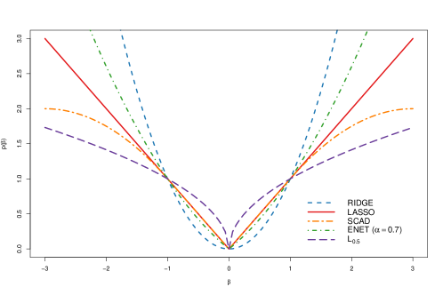
Figure 1: Comparison of different penalization methods: $L_{2}$ or RIDGE penalization ($RIDGE$), $L_{1}$ or LASSO penalization ($LASSO$), SCAD regularization ($SCAD$), Elastic Net penalization method for $\alpha=0.7$ ($ENET\;(\alpha=0.7)$) and $L_{0.5}$ regularization ($L_{0.5}$) .

The LASSO, also known as basis pursuit in image processing (chen2001atomic, candes2006stable, donoho2005stable), was presented by Tibshirani1996. This proposes the imposition of a $L_{1}$ penalization in (3) with the aim of performing variable selection and overcoming the high dimensional estimation of $\beta$ drawback when $p>n$. In this way, it would be needed to solve the optimization problem

$$\begin{split}&\hat{\beta}^{L_{1}}=\min_{\beta}\sum_{i=1}^{n}\left(y_{i}-\sum_{j=1}^{p}x_{ij}\beta_{j}\right)^{2},\\ &\text{subject to}\sum_{j=1}^{p}|{\beta_{j}}|\leq t,\end{split}$$

which can be rewritten like

$$\hat{\beta}^{L_{1}}=\min_{\beta}\left\{\sum_{i=1}^{n}\left(y_{i}-\sum_{j=1}^{p}x_{ij}\beta_{j}\right)^{2}+\lambda\sum_{j=1}^{p}|{\beta_{j}}|\right\}.$$ (6)

The problem (6) is convex, which guarantees that has always one solution at least, although if $p>n$, there may be multiple minimums (see tibshirani2013LASSO for more details). Besides, assuming the noise term $\varepsilon$ to be Gaussian, $\hat{\beta}^{L_{1}}$ can be interpreted as a penalized maximum likelihood estimate in which the fitted coefficients are penalized in a $L_{1}$ sense. As a result, this encourages sparsity.

In these problems, the term $\lambda>0$, or $t>0$ equivalently, is the shrinkage parameter. For large values of $\lambda$ (small values of $t$) the coefficients of $\beta$ are more penalized, which results in a bigger number of elements shrinkaged to zero. Nevertheless, the estimator $\hat{\beta}^{L_{1}}$ of (6) has not got an explicit expression.

The LASSO defined in (6) can be viewed as a convex relaxation of the optimization problem with the $L_{0}$ analogue of a norm in (5). Then, the requirement of computational feasibility and statistical accuracy can be met by this estimator.

This method has been widely studied over the last years: it has been showed that this procedure is consistent in terms of prediction (see van2009conditions for an extensive analysis) and this guarantees consistency of the parameter estimates at least in a $L_{2}$ sense (van2009conditions, meinshausen2009LASSO, candes2007dantzig); besides, this is a consistent variable selector under some assumptions (Meinshausen2006, wainwright2009sharp, Zhao2006).

2.1 Analysis of the LASSO regression requirements and inconveniences

In spite of all these good qualities, the LASSO regression has some important limitations in practice (see for example Zou2005 or Su2017). These limitations are analyzed in the next subsections, collecting some recent developed theoretical properties and displaying how far it is possible to ensure its good behavior.

2.1.1 Biased estimator

In the context of having more covariates $p$, than number of samples $n$, the LASSO regression can identify at most $n$ important covariates before it saturates (see Zou2005). This restriction is common for almost all regression adjustment methods which rely on penalizations in this framework. Specially for those based on $L_{1}$ ideas. As a result, an estimator $\hat{\beta}$ can have at most $n$ coefficients not equal zero. Into words, there is not enough available information to adjust the whole model. This situation can be compared with a system of equations in which we have more variables than equations per se.

Related with this, another caveat of penalization processes is the bias. This produces higher prediction errors. In the LASSO adjustment, the imposition of the $L_{1}$ penalization in the OLS problem (3) as a safe passage to estimate $\beta$ has a cost, which is translated in bias (see hastie2009elements, giraud2014introduction or hastie2015statistical). This can be easily explained under orthogonal design, where the $L_{1}$ penalization results in a perturbation of the unbiased OLS estimator $\hat{\beta}^{OLS}$ given by

$$\hat{\beta}^{L_{1}}_{j}=\textrm{sign}(\hat{\beta}_{j}^{OLS})(|\hat{\beta}_{j}^{OLS}|-\lambda)_{+},$$ (7)

where $\textrm{sign}(\cdot)$ denotes the sign of the coefficients and $(\cdot)_{+}$ equals to zero all quantities which are not positive. This results in a soft threshold of the ordinary mean square estimator ruled by the $\lambda>0$ parameter, where the coefficients $|\hat{\beta}^{OLS}_{j}|\leq\lambda$ are adjusted to zero.

In order to correct the bias, weighted versions of the LASSO method based on iterative schemes, have been developed. An example is the popular adaptive LASSO (Zou2006, huang2008adaptive, Geer2011). This procedure gives different weights to each covariate in the penalization part, readjusting these in every step of the iterative process until convergence.

2.1.2 Consistency of the LASSO: neighborhood stability condition

Despite the LASSO is broadly employed, it is not always possible to guarantee its proper performance. As we can see in buhlmann2011statistics, certain conditions are required to guarantee an efficient screening property for variable selection. However, this presents some important limitations as a variable selector when these do not hold.

For example, when the model has several highly correlated covariates with the response, LASSO tends to pick randomly only one or a few of them and shrinks the rest to $0$ (see Zou2005). This fact results in a confusion phenomenon if there are high correlations between relevant and unimportant covariates, and in a loss of information when the subset of important covariates have a strong dependence structure. Some algorithms which result in non-sparse estimators try to relieve this effect, like the Ridge regression (hoerl1970ridge) or the Elastic Net (Zou2005). An interpretation of their penalties is displayed in Figure 1.

Denoting $S=\{j:\beta_{j}\not=0\}$ the set of non-zero real values and estimating this by $\hat{S}$, this last would be a consistent estimator if this verifies

$$\mathbb{P}(\hat{S}=S)\stackbin[n\rightarrow\infty]{}{\longrightarrow}1.$$ (8)

The condition (8) places a restriction on the growth of the number $p$ of variables and sparsity $|S|$, typically of the form $|S|\log(p)=o(n)$ (see Meinshausen2006). Denoting $s=|S|$, this forces the necessity of $n>s\log(p)$ in order to achieve consistency for the LASSO estimator.

Besides, for consistent variable selection using $\hat{S}^{L_{1}}=\{j:\hat{\beta}^{L_{1}}_{j}\not=0\}$, it turns out that the design matrix of the model, $X$, needs to satisfy some assumptions. The strongest of which is arguably the so-called “neighborhood stability condition” (Meinshausen2006). This condition is equivalent to the irrepresentable condition (Zhao2006; Zou2006; Yuan2007):

$$\max_{j\in S^{c}}|\textrm{sign}(\beta_{S})^{\top}(X_{S}^{\top}X_{S})^{-1}X_{S}^{\top}X_{j}|\leq\theta\quad\text{for some }0<\theta<1,$$ (9)

being $\beta_{S}$ the subvector of $\beta$ and $X_{S}$ the submatrix of $X$ considering the elements of $S$.

If this condition is violated, all that we can hope for is recovery of the regression vector $\beta$ in an $L_{2}$-sense of convergence by achieving $\parallel\hat{\beta}^{L_{1}}-\beta\parallel_{2}\stackbin[n\rightarrow\infty]{}{\longrightarrow_{p}}0$ (see Meinshausen2010 for more details). Moreover, under some assumptions in the design, the irrepresentable condition can be expressed as the called “necessary condition” (Zou2006). It is not an easy task to verify these conditions in practice, specially in contexts where $p$ can be huge.

Quoted buhlmann2011statistics: roughly speaking, the neighborhood stability or irrepresentable condition (9) fails to hold if the design matrix $X$ is too much “ill-posed” and exhibits a too strong degree of linear dependence within “smaller” sub-matrices of X.

In addition, it is needed to assure that there are enough information and suitable characteristics for “signal recovery” of the sparse $\beta$ vector. This requires relevant covariates coefficients be large enough so as to distinguish them from the zero ones. Then, the non-zero regression coefficients need to satisfy

$$\stackbin[j\in S]{}{\inf}|\beta_{j}|>>\sqrt{s\log(p)/n}$$ (10)

in order to guarantee the consistency of the $\hat{\beta}^{L_{1}}$ estimator of problem (6). This is called a beta-min condition. Nevertheless, this requirement may be unrealistic in practice and small non-zero coefficients may not be detected (in a consistent way). See buhlmann2011statistics for more information.

Owing to these difficulties, different new methodologies based on ideas derived from subsampling and bootstrap have been developed. Examples are the random LASSO (wang2011random), an algorithm based on subsampling, or the stability selection method mixed with randomized LASSO of Meinshausen2010. This last searches for consistency although the irrepresentable condition introduced in (9) would be violated.

2.1.3 False discoveries of the LASSO

As it is explained in Su2017: In regression settings where explanatory variables have very low correlations and there are relatively few effects, each of large magnitude, we expect the LASSO to find the important variables with few errors, if any. Nevertheless, in a regime of linear sparsity, there exist a trade-off between false and true positive rates along the LASSO path, even when the design variables are stochastically independent. Besides, this phenomenon occurs no matter how strong the effect sizes are.

This can be translated as one of the major disadvantages of using LASSO like a variable selector is that exists a trade-off between the false discovery proportion (FDP) and the true positive proportion (TPP), which are defined as

$$FDP(\lambda)=\frac{F(\lambda)}{|\{j:\hat{\beta}_{j}(\lambda)\not=0\}|\vee 1}\quad\text{and}\quad TPP(\lambda)=\frac{T(\lambda)}{s\vee 1},$$ (11)

where $F(\lambda)=|\{j\in S^{c}:\hat{\beta}_{j}(\lambda)\not=0\}|$ denotes the number of false discoveries, $T(\lambda)=|\{j\in S:\hat{\beta}_{j}(\lambda)\not=0\}|$ is the number of positive discoveries and $a\vee b=\max\{a,b\}$.

Then, it is unlikely to achieve high power and a low false positive rate simultaneously. Noticing that $FDP$ is a natural measure of type I error while $1-TPP$ is the fraction of missed signals (a natural notion of type II error), the results say that nowhere on the LASSO path can both types of error rates be simultaneously low. This also happens even when there is no noise in the model and the regressors are stochastically independent. Hence, there exists only a possible reason: it is because of the $L_{1}$ shrinkage which results in pseudo-noise. Furthermore, this does not occur with other types of penalizations, like the $L_{0}$ penalty. See Su2017 for more details.

In fact, it can be proved in a quiet global context, that the LASSO is not capable of selecting the correct subset of important covariates without adding some noise to the model in the best case (see wasserman2009high or Su2017).

Then, modifications of the traditional LASSO procedure are needed in order to control the FDP. Some alternatives, such as the boLASSO procedure (see Bach2008), which use bootstrap to calibrate the $FDP$, the thresholded LASSO (Zhou2010), based on the use of a threshold to avoid noise covariates, or more recent ones, like the stability selection method (see Meinshausen2010) or the use of knockoffs (see Hofner:StabSel:2015, Weinstein2017, candes2018panning and barber2019knockoff), were proposed to solve this drawback. To the best of our knowledge still there is not a version of this last for the $p>n$ framework.

2.1.4 Correct selection of the penalization parameter $\boldsymbol{\lambda}$

One of the most important parts of a LASSO adjustment is the proper selection of the penalization parameter $\lambda\geq 0$. Its size controls both: the number of selected variables and the degree to which their estimated coefficients are shrunk to zero, controlling the bias as well. A too large value of $\lambda$ forces all coefficients of $\hat{\beta}^{L_{1}}$ to be null, while a value next to zero includes too many noisy covariates. Then, a good choice of $\lambda$ is needed in order to achieve a balance between simplicity and selection accuracy.

The problem of the proper choice of the $\lambda$ parameter depends on the unknown error variance $\sigma^{2}$. We can see in buhlmann2011statistics that the oracle inequality states to select $\lambda$ of order $\sigma\sqrt{\log(p)/n}$ to keep the mean squared prediction error of LASSO as the same order as if we knew the active set $S$ in advance. In practice, the $\sigma$ value is unknown and its estimation with $p>n$ is quite complex. To give some guidance in this field we refer to fan2012variance or reid2016study, although this still is a growing study field.

Thus, other methods to estimate $\lambda$ are proposed. Following the classification of homrighausen2018study we can distinguish three categories: minimization of a generalized information criteria (like AIC or BIC), by means of resampling procedures (such as cross-validation or bootstrap) or reformulating the LASSO optimization problem. Due to computational cost, the most used criteria to fit a LASSO adjustment are cross-validation techniques. Nevertheless, it can be showed that this criterion achieves an adequate $\lambda$ value for prediction risk but this leads to inconsistent model selection for sparse methods (see Meinshausen2006). Then, for recovering the set $S$, a larger penalty parameter would be needed (buhlmann2011statistics).

Su2017 argue that, when the regularization parameter $\lambda$ is needed to be large for a proper variable selection, the LASSO estimator is seriously biased downwards. The residuals still contain much of the effects associated with the selected variables, which is called shrinkage noise. As many strong variables get picked up, this gets inflated and its projection along the directions of some of the null variables may actually dwarf the signals coming from the strong regression coefficients, selecting null variables.

Nevertheless, to the best of our knowledge, there is not a common agreement about the way of choosing this $\lambda$ value. Hence, cross-validation techniques are widely used to adjust the LASSO regression. See homrighausen2018study for more details.

3 A comparative study with simulation scenarios

Once the LASSO requirements have been introduced, its performance is tested in practice. So, scenarios verifying and do not these conditions, mixed with different dependence structures, are simulated to compare its results with those of other procedures. For this purpose, a Monte Carlo study is carried out. Three different interesting dependence scenarios are introduced, simulating them under the linear regression model structure given by (2). We consider $\beta$ as a sparse vector of length $p$ with only $s<p$ values not equal zero and $X\in\mathbb{R}_{n\times p}$, where $n$ is the sample size. It is assumed that $\varepsilon\in N_{n}(0,\sigma^{2}I_{n})$, so once a value for $\sigma^{2}$ is provided, we can obtain $Y$. We fix $p=100$ and choose $\sigma^{2}$ verifying that the percentage of explained deviance is explicitly the $90\%$. Calculation of this parameter is collected in Section 1 of the Supplementary material. Then, to guarantee the conditions introduced in Sections 2.1.2, 2.1.3 and 2.1.4, it is needed that $n>4.61s$ as we saw in (8), $\inf|\beta_{j}|>>2.15\sqrt{s/n}$ for $j\in S$ as in (10) and $\lambda\sim 2.15\sigma\sqrt{1/n}$. To test their performance under these conditions and when they are violated, we consider different combinations of parameters values taking $n=25,50,100,200,400$ and $s=10,15,20$. A study of when these conditions hold is showed in Section 2 of the Supplementary material. In every simulation, we count the number of covariates correctly selected ($|\hat{S}\cap S|$) as well as the noisy ones ($|\hat{S}\setminus S|$). Besides, we measure the prediction power of the algorithm by means of the percentage of explained deviance ($\%Dev$) and the mean squared error ($MSE$). This last gives us an idea about the bias produced by the LASSO (see Section 2.1.1). We repeat this procedure a number $M=500$ of times and compute on average its results.

• Scenario 1 (Orthogonal design). Only the first $s$ values are not equal zero for $\beta_{j}$ with $j=1,\dots,s$ and $p>s>0$, $\beta_{1}=\dots=\beta_{s}=1.25$, while $\beta_{j}=0$ for all $j=s+1,\dots,p$. $X$ is simulated as a $N_{n}(0,I_{p})$.

• Scenario 2 (Dependence by blocks). The vector $\beta$ has the first $s<p$ components not null, of the form $\beta_{1}=\dots=\beta_{s}=1$ and $\beta_{j}=0$ for the rest. $X$ is simulated as a $N_{n}(0,\Sigma)$, where $\sigma_{jj}=1$ and $\sigma_{jk}=cov(X_{j},X_{k})=0$ for all pairs $(j,k)$ except if $mod_{10}(j)=mod_{10}(k)$, in that case $\sigma_{jk}=\rho$, taking $\rho=0.5,0.9$.

• Scenario 3 (Toeplitz covariance). Again, only $s$ ($p>s>0$) covariates are important, simulating $X$ as a $N_{n}(0,\Sigma)$ and assuming $\beta_{j}=0.5$ in the places where $\beta\not=0$. In this case, $\sigma_{jk}=\rho^{|j-k|}$ for $j,k=1,\dots,p$ and $\rho=0.5,0.9$. Now, we analyze two different dependence structures varying the location of the $s$ relevant covariates:

  • Scenario 3.a: we assume that the relevant covariates are the first $s=15$.

  • Scenario 3.b: consider $s=10$ relevant variables placed every 10 sites, which means that only the $\beta_{1},\beta_{11},\beta_{21},\dots,\beta_{91}$ terms of $\beta$ are not null.

The first choice, the orthogonal design of Scenario 1, is selected as the best possible framework. This verifies the consistency conditions for values of $n$ large enough and avoids the confusion phenomenon given that there are not correlated covariates.

In contrast, to assess how the LASSO behaves in case of different dependence structures, Scenario 2 and Scenario 3 are proposed. In the dependence by blocks context (Scenario 2), we force the design to have a dependence structure where the covariates are correlated ten by ten. As a result, we induce a more challenging scenario for the LASSO, in which the algorithm has to overcome a fuzzy signal produced by irrelevant covariates. Different magnitudes of dependence are considered in Scenario 2 with $\rho=0.5$ and $\rho=0.9$ to test the effect of the confusion phenomenon. As a result, different sizes of $n$ are needed in terms of $s$ to guarantee the proper behavior of the LASSO. This scenario has been studied in other works, like in Meinshausen2010.

Eventually, the LASSO performance is tested in a scenario were all the covariates are correlated: the Toeplitz covariance structure (Scenario 3). This mimics a time series dependence pattern. This is an example where the irrepresentable condition holds but the algorithm suffers from highly correlated relations between the true set of covariates and unimportant ones. This framework has been studied for the LASSO case, see for example Meinshausen2010 or buhlmann2011statistics. Because the distance between covariates is relevant to establish their dependence, we study two different frameworks. In the first scenario (Scenario 3.a) the important covariates are highly correlated among them and little with the rest. Particularly, there are only notable confusing correlations in the case of the last variables of $S=\{1,\dots,15\}$ with their noisy neighbors. Here, the LASSO is only able to recover $S$ in the $n=400$ case. In contrast, in the Scenario 3.b, the important covariates are markedly correlated with unimportant ones, contributing to magnify the spurious correlations phenomenon. For this scenario we need a size of $n=200,400$.

We start testing the performance of the standard LASSO using the library glmnet (Friedman2010) implemented in R (R). This uses K-fold cross-validation to select the $\lambda$ parameter. As it was explained in Section 2.1.4, this is one of the most popular ways of estimating $\lambda$. In order to be capable of comparing different models and following recommendations of the existing literature, we have fixed $K=10$ for all simulations. Besides, we work with the response $y$ centered and with the matrix $\mathbf{X}$ standardized by columns. This last would not be really necessary in these frameworks because the covariates are all in the same scale. However, this is done to keep the usual implementation of LASSO type algorithms in practice. We apply a first screening step and then we adjust a linear regression model with the selected covariates. This scheme is also following for the rest of procedures.

There are other faster algorithms available in R, such as the famous LARS procedure (efron2004least, lars_R). However, we decided to make use of the glmnet library due to its easy implementation and interpretation, as well as its simple adaptation to other derivatives of the LASSO we test in this document.

3.1 Performance of the LASSO in practice

In order to test the inconveniences of the LASSO when there exists dependence among covariates, a complete simulation study is carried out. For this purpose, we make use of the simulation scenarios introduced above. Complete results are displayed in the Section 4 of the Supplementary material.

In the orthogonal design of Scenario 1, we would expect the LASSO to recover the whole set of important covariates and not to add too much noise into the model for a large enough value of $n$. However, we have observed different results.

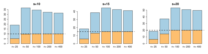
Figure 2: Number of important covariates (orange area) versus noisy ones (blue area) selected by the LASSO in Scenario 1. The dashed line marks the $s$ value.

Firstly, we can appreciate that it does not really matter the number of relevant covariates considered ($s=10,15,20$) in relation with the capability of recovering this set. It is because the algorithm only includes the complete set under the $n\geq p$ framework except for the $s=10$ scenario taking $n=50$. See this fact in Figure 2. It can be easily explained in terms of the consistence requirements of the LASSO given in (8). Besides, although we are under orthogonal design assumption, this includes a lot of noisy variables in the model. What is shocking is the fact that the number of irrelevant covariates selected is always larger than the important ones. This exemplifies the existing trade-off between FDP and TPP introduced in (11) as well as that both quantities can not be simultaneously low.

	$\mathbf{s=10}$		$\mathbf{s=15}$		$\mathbf{s=20}$
	MSE $(1.736)$	% Dev	MSE $(2.604)$	% Dev	MSE $(3.472)$	% Dev
$n=50$	0.18	0.989	0.517	0.977	1.668	0.947
$n=100$	0.701	0.959	0.846	0.967	0.916	0.973
$n=200$	1.164	0.932	1.624	0.936	2.060	0.94

Table 1: Summary of the LASSO results for Scenario 1. The oracle value for the deviance is $0.9$ and those for the MSE are in brackets.

In second place, we notice that this procedure clearly overestimates its results. This obtains values for the MSE and percentage of explained deviance less and greater, respectively, of the oracle ones (see values in brackets in Table 1). In conclusion, with this toy example we can illustrate how the LASSO procedure performs very poorly and present important limitations even in an independence framework.

Next, we analyze the results of the dependence by blocks context. In case of dependence, it is expected for a “smart” algorithm to be capable of selecting a portion of relevant covariates and explaining the remaining ones making use of the existing correlation structure. The subset of $S$ which is really necessary to explain this type of models is denote as “effective covariates”. These can be calculated measuring how many are necessary to explain a certain percentage of $\Sigma_{S}$ variability, being $\Sigma_{S}$ the submatrix of $\Sigma$ considering the elements of $S$. This number is inversely proportional to the dependence strength. For example, to explain the $90-95\%$, we found that for the Scenario 2 with $\rho=0.5$ there are needed about $12-14$ covariates taking $s=15$ and about $16-18$ for the case of $s=20$. In contrast, only $10$ are necessary in Scenario 2 with $\rho=0.9$. Complete calculation for the different simulation scenarios is displayed in Section 3 of the Supplementary material. Again, the LASSO presents some difficulties for an efficient recovery.

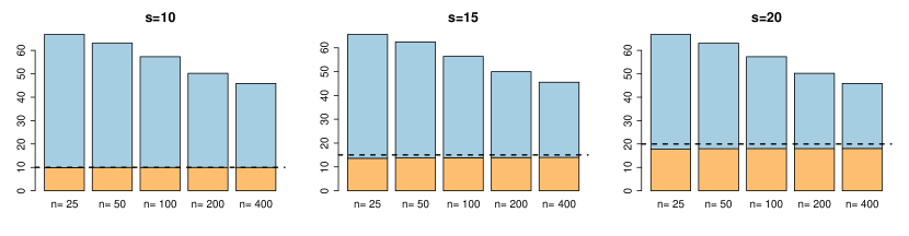
Figure 3: Number of important covariates (orange area) versus noisy ones (blue area) selected by the LASSO in Scenario 2 with $\rho=0.5$. The dashed line marks the $s$ value.

	$\mathbf{s=10}$		$\mathbf{s=15}$		$\mathbf{s=20}$
	MSE $(0.556)$	% Dev	MSE $(1.389)$	% Dev	MSE $(2.222)$	% Dev
$n=50$	0.438	0.956	1.095	0.956	1.752	0.956
$n=100$	0.495	0.951	1.238	0.951	1.981	0.951
$n=200$	0.523	0.951	1.307	0.950	2.091	0.951

Table 2: Summary of the LASSO results for Scenario 2 with $\rho=0.5$. The oracle value for the deviance is $0.9$ and those for the MSE are in brackets.

A summary of the results for the Scenario 2 with $\rho=0.5$ is displayed in Table 2 and Figure 3, while for the Scenario 2 with $\rho=0.9$ is showed in Table 3 and Figure 4. If we consider only $s=10$ important explanatory variables, its behavior is quite similar to the Scenario 1. Besides, in both scenarios with $s=10$, LASSO almost recovers the complete set $S$, even for $n=25$ although its proper recovery is guaranteed from $n=50$. However, more noise is included in this last.

Figure 4: Number of important covariates (orange area) versus noisy ones (blue area) selected by the LASSO in Scenario 2 with $\rho=0.9$. The dashed line marks the $s$ value.

	$\mathbf{s=10}$		$\mathbf{s=15}$		$\mathbf{s=20}$
	MSE $(1)$	% Dev	MSE $(2.5)$	% Dev	MSE $(4)$	% Dev
$n=50$	0.784	0.926	1.96	0.925	3.137	0.926
$n=100$	0.888	0.918	2.22	0.918	3.551	0.918
$n=200$	0.939	0.913	2.347	0.913	3.756	0.913

Table 3: Summary of the LASSO results for Scenario 2 with $\rho=0.9$. The oracle value for the deviance is $0.9$ and those for the MSE are in brackets.

In contrast, the situation is different if we simulate with $s=15$ or $s=20$ relevant covariates. Then, the LASSO does not tend to recover the covariates of $S$, not even for values of $n$ verifying $n\geq p$ as well as conditions (8) and (10). See Section 2 of the Supplementary material for more information. However, this selects more than the effective number of covariates. It seems the LASSO tries to recover the set $S$ but, due to the presence of spurious correlations, this chooses randomly between two highly correlated important covariates. It can be appreciated in Figures LABEL:barplots_M2_25_rho_5-LABEL:barplots_M2_clases_rho_9 of the Appendix that the $10$ first covariates are selected with high probability, near $1$, but due to the confusion phenomenon some of them are interchanged by a representative one. The following $s-10$ relevant variables have a lower selection rate and there are some irrelevant ones selected a larger number of times, adding quite noise to the model. This inconvenient seems not to be overcome increasing the number of samples $n$. Again, the LASSO keeps overestimating its results as we can see by the percentage of explained deviance and the MSE.

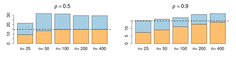
Figure 5: Number of important covariates (orange area) versus noisy ones (blue area) selected by the LASSO in Scenario 3.a. The dashed line marks the $s$ value.

	$\boldsymbol{\rho=0.5}$		$\boldsymbol{\rho=0.9}$
	MSE $(1.139)$	% Dev	MSE $(3.807)$	% Dev
$n=50$	0.19	0.983	1.894	0.950
$n=100$	0.546	0.951	2.815	0.928
$n=200$	0.825	0.927	3.302	0.916

Table 4: Summary of the LASSO results for Scenario 3.a. The oracle value for the deviance is $0.9$ and those for the MSE are in brackets.

Finally, we study the results of the Toeplitz covariance structure by means of the Scenario 3.a, where the relevant covariates are the first $s=15$ (Table 4 and Figure 5), and the Scenario 3.b, where there are only $s=10$ important variables placed every 10 sites (Table 5 and Figure 6).

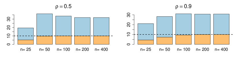
Figure 6: Number of important covariates (orange area) versus noisy ones (blue area) selected by the LASSO in Scenario 3.b. The dashed line marks the $s$ value.

Interpreting their results, we see that the LASSO procedure recovers the important set of covariates for $\rho=0.5$, taking a value of $n=100,200,400$ verifying the consistent condition, in both cases. Nevertheless, this exceeds the number of efficient covariates in Scenario 3.a for $\rho=0.9$ and in the two cases of Scenario 3.b, because with $10$ covariates it is explained the $98\%$ of variability. Moreover, this algorithm returns to include many pointless covariates in the model and overestimates the prediction accuracy.

	$\boldsymbol{\rho=0.5}$		$\boldsymbol{\rho=0.9}$
	MSE $(0.278)$	% Dev	MSE $(0.53)$	% Dev
$n=50$	0.034	0.987	0.147	0.971
$n=100$	0.123	0.955	0.309	0.94
$n=200$	0.195	0.929	0.417	0.920

Table 5: Summary of the LASSO results for Scenario 3.b. The oracle value for the deviance is $0.9$ and those for the MSE are in brackets.

4 Evolution of the LASSO in the last years and alternatives

Once the LASSO and its inconveniences have been displayed, we want to compare its performance with other approaches. Then, we test different methodologies designed to select the relevant information and adjust a regression model in the $p>n$ framework. Nevertheless, it is impossible to include all the existing algorithms here. Instead, we attempted to collect the most relevant ones, providing a summary of the most used methodologies nowadays.

Methods proposed to alleviate the limitations of the LASSO algorithm are based in a wide range of different philosophies. Some of them opt to add a second selection step after solving the LASSO problem, such as the relaxed LASSO (meinshausen2007relaxed) or thresholded LASSO (Zhou2010, Geer2011), while other alternatives are focused on giving different weights to the covariates proportional to their importance, as the adaptive LASSO (Zou2006, huang2008adaptive, Geer2011). Others pay attention to the group structure of the sparse vector $\beta$ when this exists, like the grouped LASSO procedure (yuan2006model) or the fused LASSO (tibshirani2005sparsity).

The resampling or iterative procedures are other approaches which make use of subsampling or computational power, algorithms like boLASSO (Bach2008), stability selection with randomized LASSO (Meinshausen2010), the random LASSO (wang2011random), the scaled LASSO (sun2012) or the combination of classic estimators with variable selection diagnostics measures (nan2014variable), among others, are based on this idea. Furthermore, more recent techniques like the Knockoff filter (Barber2015, candes2018panning) or SLOPE (Bogdan2015) have been introduced to control some measures of the type I error. One drawback of the famous Knockoff filter is that, to the best of our knowledge, this is not yet available for the $p>n$ case.

There are other alternatives, which modify the constraints of the LASSO problem (6) so as to achieve better estimators of $\beta$, like the Elastic Net (Zou2005), the Dantzig selector (candes2007dantzig, bickel2009simultaneous) or the square root LASSO (belloni2011square). Moreover, other different alternatives have been developed recently, such as the Elem-OLS Estimator (yang2014elementary), the LASSO-Zero (descloux2018model) or the horseshoe (bhadra2019LASSO), adding new ideas to the previous list.

Quoted descloux2018model: although differing in their purposes and performance, the general idea underlying these procedures remains the same, namely to avoid overfitting by finding a trade-off between the fit $y-X\beta$ and some measure of the model complexity.

Along the many papers, we have found that a modest classification of the different proposals can be done, although in this classification some of the procedures does not only fit in a single class. These categories are

• Weighted LASSO: weighted versions of the LASSO algorithm with a suitable selection of the weights. They are proposed to attach the particular importance of each covariate in the estimation process. Besides, joint with iteration, this modification allows a reduction of the bias.

• Resampling LASSO procedures: mix of the typical LASSO adjustment with resampling procedures, based, for example, on randomization in the selection process of covariates so as to reduce unavoidable random noise.

• Thresholded versions of the LASSO: a second thresholding step in the covariates selection is implemented in order to reduce the irrelevant ones.

• Alternatives to the LASSO: procedures with different nature and aims designed to solve the LASSO drawbacks.

This extensive list of procedures makes noticeable the impact the LASSO has nowadays. A brief summary is displayed in Table LABEL:table_other.

Owing to the computational cost required for the resampling LASSO procedures, such as the boLASSO of Bach2008 or the random LASSO algorithm (wang2011random), these algorithms are too slow. Even for small values of $p$, we found that the computational costs were high. For this reason, they are excluded for the comparative analysis studio. The LASSO-Zero technique of descloux2018model suffers from the same issue, so it is excluded too.

Other problem springs up for the thresholded versions of the LASSO. In this case, we noticed that the complexity of finding a correct threshold is similar to the one of obtaining the optimal value of $\lambda$ for the LASSO adjustment. In both cases, we would need to know in advance the dispersion of the error $\sigma^{2}$, which is usually impossible in practice. Then, procedures as the thresholded LASSO algorithm of Zhou2010 are shut out in order to not add more complications to the adjustment.

One method in the middle of both groups is the stability selection procedure proposed by Meinshausen2010. This methodology pays attention to the probability of each covariate to be selected. Only the covariates with probability greater than a fixed threshold are added to the final model. We have observe in practice that a proper choice of the threshold value seems to depend on the sample size considered, $n$, as well as the sparsity of the vector $\beta$. An example is showed simulating the stability selection procedure using the standard LASSO in Scenario 1 with $s=10$ (Figure LABEL:threshold_s_10). Eventually, it is interesting to take into account that it seems no possible to guarantee consistency for any thresholding value in case that $n>p$. For this reason, this approach is not included in the comparison neither.