TESS Asteroseismology of $\alpha$ Mensae: Benchmark Ages for a G7 Dwarf and its M-dwarf Companion

Abstract

Asteroseismology of bright stars has become increasingly important as a method to determine fundamental properties (in particular ages) of stars. The Kepler Space Telescope initiated a revolution by detecting oscillations in more than 500 main-sequence and subgiant stars. However, most Kepler stars are faint, and therefore have limited constraints from independent methods such as long-baseline interferometry. Here, we present the discovery of solar-like oscillations in $\alpha$ Men A, a naked-eye (V = 5.1) G7 dwarf in TESS’s Southern Continuous Viewing Zone. Using a combination of astrometry, spectroscopy, and asteroseismology, we precisely characterize the solar analogue $\alpha$ Men A ($T_{\mathrm{eff}}$ = 5569 $\pm$ 62 K, $R_{\star}$ = 0.960 $\pm$ 0.016 $R_{\odot}$, $M_{\star}$ = 0.964 $\pm$ 0.045 $M_{\odot}$). To characterize the fully-convective M-dwarf companion, we derive empirical relations to estimate mass, radius and temperature given the absolute Gaia magnitude and metallicity, yielding $M_{\star}$ = $0.169\pm 0.006$ $M_{\odot}$, $R_{\star}$ = $0.19\pm 0.01$ $R_{\odot}$ and $T_{\mathrm{eff}}$ = $3054\pm 44$ K. Our asteroseismic age of 6.2 $\pm$ 1.4 (stat) $\pm$ 0.6 (sys) Gyr for the primary places $\alpha$ Men B within a small population of M dwarfs with precisely measured ages. We combined multiple ground-based spectroscopy surveys to reveal an activity cycle of $P$ = 13.1 $\pm$ 1.1 years for $\alpha$ Men A, a period similar to that observed in the Sun. We used different gyrochronology models with the asteroseismic age to estimate a rotation period of $\sim$30 days for the primary. Alpha Men A is now the closest (d = 10 pc) solar analogue with a precise asteroseismic age from space-based photometry, making it a prime target for next-generation direct imaging missions searching for true Earth analogues.

1 Introduction

Accurate ages are essential for stellar astrophysics but arguably the most difficult fundamental property to determine. Galactic archaeology uses stellar ages to reconstruct the formation history of the Milky Way Galaxy, while ages of exoplanet host stars are important to explain the diverse population of exoplanets observed today. Furthermore, ages will be important for next-generation space-based missions looking to image Earth-like planets orbiting Sun-like stars. For example, future imaging missions would greatly benefit from an age-based target selection when attempting to identify biosignatures in the context of exoplanet habitability (Bixel & Apai, 2020).

There are many techniques to estimate stellar ages but no single method suitable for all spectral types (Soderblom, 2010). The most widely used is isochrone fitting, which is most fruitful for stellar clusters, where the main-sequence turnoff provides an age for an ensemble of stars. Isochrones also typically produce reliable ages for massive stars ($\gtrsim$1.5$M_{\odot}$) or stars on the subgiant branch, for which stellar evolution is relatively quick. However, determining the ages of field stars is difficult, particularly for low-mass dwarfs that spend most of their lifetime on the main sequence. Consequently, many studies have focused on finding empirical relations between physically-motivated age indicators and other observables in lower main sequence stars.

Early disk-integrated Ca ii H and K fluxes of the Sun revealed variations that correlated with the activity cycle, leading to one of the first empirical age relations. Activity in the Sun is generated through the magnetic dynamo mechanism, whose efficiency depends on subsurface convection and differential rotation (Kraft, 1967). Pioneering work by Wilson (1978) observed these two chromospheric emission lines for nearly 100 cool main-sequence stars and demonstrated that many stars have cyclic variations analogous to that found in the Sun. In addition, studies of open clusters revealed an inverse relationship between stellar age and activity (Wilson, 1963, 1966; Skumanich, 1972; Soderblom et al., 1991). An empirical relation between chromospheric activity and age was established and would ultimately be the leading age indicator for later-type field stars for decades (Noyes et al., 1984; Baliunas et al., 1995; Henry et al., 1996; Wright et al., 2004).

Another empirical relation uses stellar rotation periods to estimate ages based on the spindown of stars with time (gyrochronology). This mechanism is enabled by magnetic braking, where charged particles escape through magnetized winds, leading to mass and angular momentum loss (Skumanich, 1972). Factoring in a mass (or color) dependence, Barnes (2007) derived an empirical rotation-age relation that successfully reproduced ages of young clusters to better than 20%. Gyrochronology recently underwent a resurgence with Kepler (Borucki et al., 2010) through the measurement of rotation periods for more than 30,000 main-sequence stars (Nielsen et al., 2013; Reinhold et al., 2013; McQuillan et al., 2014; Santos et al., 2019).

The success of empirical age relations makes it critical to verify them with independent calibrations. Recently, gyrochronology relations have failed to reproduce rotation rates for intermediate age clusters from K2, suggesting that the standard formalism needs to be adjusted (Curtis et al., 2019; Douglas et al., 2019). Moreover, van Saders et al. (2016) proposed a weakened braking law to explain the unexpected rapid rotation in older stars, indicating an additional source of uncertainty for rotation-based ages. This is further complicated for low-mass dwarfs that barely evolve over the nuclear time scale, and hence are also challenging to age through isochrones. Therefore, ages for lower main-sequence stars remain challenging and limited, which is largely due to the lack of calibrators in this regime.

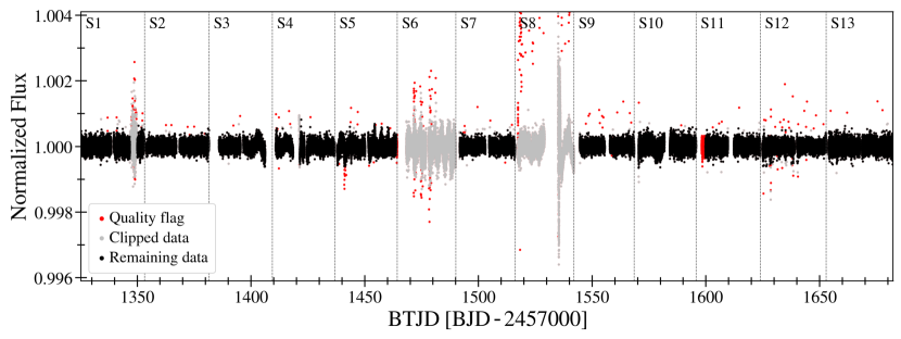
Figure 1: Normalized TESS light curve of $\alpha$ Mensae A. Red points were removed based on quality flag information, grey points were clipped according to Chontos et al. (2019), and the remaining black points ($\sim$75% of the original data) were used in the asteroseismic analysis. Dashed lines delineate the 13 sectors.

A powerful method to determine accurate ages of field stars is asteroseismology, especially for solar-like oscillations driven by near-surface convection. Kepler revolutionized the field, but only detected oscillations in $\sim$500 main-sequence and subgiant stars, most of which are quite faint (Chaplin et al., 2014; García & Ballot, 2019). The Transiting Exoplanet Survey Satellite (TESS; Ricker et al., 2015) is now targeting much brighter stars (e.g. Chaplin et al., 2020) for which we also have long-term activity monitoring, enabling the opportunity to add benchmark calibrators for alternative age determination methods.

Table 1: Literature sources for spectroscopic $T_{\mathrm{eff}}$, $\log g$, and [Fe/H] values discussed in Section 2.2.

Source	$T_{\mathrm{eff}}$ [K]	$\log g$ [cgs]	[Fe/H]
Santos et al. (2001)	$5620$	$4.56$	$0.12$
Bensby et al. (2003)	$5550$	$4.38$	$0.10$
Santos et al. (2004)	$5594$	$4.41$	$0.10$
Valenti & Fischer (2005)	$5587$	$4.50$	$0.09$
Bond et al. (2006)	$5557$	$4.43$	$0.06$
Ramírez et al. (2007)	$5536$	$4.50$	$0.12$
Bruntt et al. (2010)	$5570$	$4.43$	$0.15$
Casagrande et al. (2011)	$5605$
da Silva et al. (2012)	$5630$	$4.47$	$0.11$
Maldonado et al. (2012)	$5649$	$4.60$	$0.12$
Ramírez et al. (2012)	$5569$	$4.42$	$0.11$
Bensby et al. (2014)	$5517$	$4.48$	$0.07$
Maldonado et al. (2015)	$5607$	$4.51$
Luck (2018)	$5589$	$4.44$	$0.15$

Here we present the discovery of solar-like oscillations in $\alpha$ Mensae using TESS, which is now the closest solar analog with an asteroseismic detection from space. Alpha Men A is a naked-eye G7 star (V = 5.1) in TESS’s southern continuous viewing zone (SCVZ). It has an M-dwarf companion which we can now age-date using asteroseismology of the primary, making it an ideal target to age date two lower-main sequence stars and providing an invaluable nearby benchmark system.

2 Observations

2.1 TESS Photometry

Alpha Mensae falls in the TESS SCVZ and thus, was observed for the entire first year of the nominal mission. Alpha Men was observed in 2-minute cadence for all thirteen sectors, for a total baseline of 351 days. We used the light curve files produced by the TESS Science Processing Operations Center (SPOC; Jenkins et al., 2016) that were made publicly available on the Mukulski Archive for Space Telescopes (MAST).

We downloaded all SPOC 2-minute light curves and stitched individual sectors together using the SPOC-processed PDCSAP (Pre-Data Conditioning Standard Aperture Photometry) flux. Upon initial inspection of the light curve (Figure 1), we noticed two sectors with increased scatter by a factor of at least two. We suspect that this is due to instrumental systematics and therefore removed these data before further analysis. To prepare the light curve for asteroseismic analysis, bad data points were removed as described in Chontos et al. (2019), including points with poor quality flags, $>$5$\sigma$ outliers, or sharp time domain artefacts, which ultimately accounted for $\sim$25% of the data.

2.2 High-Resolution Spectroscopy

Alpha Mensae is a well-studied star, with twenty-eight different sets of spectroscopic parameters available on Simbad. Retaining only results from 1980 onwards that used high-resolution instruments, a total of fourteen independent spectroscopic parameters remained and are listed in Table 1. We adopted the values from Ramírez et al. (2012) and then added the standard deviation of literature values in quadrature with the reported formal uncertainties. The final set of atmospheric parameters for $\alpha$ Men A is $T_{\mathrm{eff}}$ = 5569 $\pm$ 50 (stat) $\pm$ 36 (sys) K, $\log g$ = 4.42 $\pm$ 0.03 (stat) $\pm$ 0.06 (sys) dex, and [Fe/H] = 0.11 $\pm$ 0.05 (stat) $\pm$ 0.03 (sys) dex (Table 2). We also checked the alpha abundances (in particular [Mg/Fe] and [Ca/Fe]) and found them to be consistent with solar values (Bensby et al., 2014).

Table 2: Primary Stellar Parameters

Other identifiers:
alf Men, HR 2261, HD 43834,
HIP 29271, Gaia DR2 5264749303461634816
Gaia eDR3 5264749303462961280, TIC 141810080
Parameter	Value	Source
Right ascension (RA), $\rm\alpha_{J2016}$	$92.5624$	1, 2
Declination (Dec), $\rm\delta_{J2016}$	$-74.7540$	1, 2
Parallax, $\pi$ (mas)	$97.9158\pm 0.0573$	1, 2
Distance, $d$ (pc)	$10.2129\pm 0.0060$	1, 2
Spectral type	G7V	3
Photometry
Tycho-2 B mag, $B_{T}$	$5.968\pm 0.014$	4
Tycho-2 V mag, $V_{T}$	$5.151\pm 0.009$	4
2MASS J mag, $J$	$3.951\pm 0.232$	5, 6
2MASS H mag, $H$	$3.508\pm 0.228$	5, 6
2MASS KS mag, $K_{S}$	$3.446\pm 0.200$	5, 6
Gaia G mag, $G^{\dagger}$	$4.8973\pm 0.0025$	1, 2
Gaia Bp mag, $Bp$	$5.2783\pm 0.0024$	1, 2
Gaia Rp mag, $Rp$	$4.3900\pm 0.0023$	1, 2
Spectroscopy & Gaia
Effective temperature, $T_{\mathrm{eff}}$ (K)	$5569\pm 50(36)$	8
Metallicity, [Fe/H] (dex)	$0.11\pm 0.05(0.03)$	8
Surface gravity, $\log g$ (cgs)	$4.42\pm 0.03(0.06)$	8
Projected rotation speed, $v\sin i$ (km s-1)	$0.6\pm 0.6$	9
Luminosity, $L_{\star}$ ($L_{\odot}$)	$0.81\pm 0.02$
Asteroseismology
Stellar mass, $M_{\star}$ ($M_{\odot}$)	$0.964\pm 0.037(0.026)$
Stellar radius, $R_{\star}$ ($R_{\odot}$)	$0.960\pm 0.013(0.009)$
Stellar density, $\rho_{\star}$ (gcc)	$1.531\pm 0.018(0.011)$
Surface gravity, $\log g$ (cgs)	$4.459\pm 0.006(0.004)$
Age, $t$ (Gyr)	$6.2\pm 1.4(0.6)$

References – (1) Gaia Collaboration et al. (2016) (2) Gaia Collaboration et al. (2021) (3) Gray et al. (2006) (4) Høg et al. (2000) (5) Cutri et al. (2003) (6) Skrutskie et al. (2006) (7) Stassun et al. (2019) (8) Ramírez et al. (2012) (9) Bruntt et al. (2010)

Note —
^† Magnitude has been corrected for saturation according to Evans et al. (2018).

2.3 Broadband Photometry & Gaia Parallax

Due to its brightness (V = 5.1) $\alpha$ Men A is saturated in many large photometric surveys. For optical magnitudes, we relied on $B_{T}$ and $V_{T}$ magnitudes from the Tycho-2 catalog (Høg et al., 2000). Cutri et al. (2012) reported reliable quality flags for $J,H,K_{S}$ photometry in the extended 2MASS catalog, although we note the higher uncertainties due to the choice of aperture needed for saturated stars. The European Space Agency’s (ESA) Gaia Data Release 2 (DR2; Gaia Collaboration et al., 2018) estimated a mean Gaia magnitude $G$ = 4.850 for alpha Men. Brighter sources in DR2 photometry ($G$ $<$ 6) suffer from systematic errors due to saturation (Evans et al., 2018). Using the empirical correction in Evans et al. (2018), we calculated a corrected Gaia magnitude, $G$ = 4.897. The new Gaia eDR3 catalog reported a value of $G$ = 4.900 for the primary and is therefore consistent with the corrected magnitude used in this analysis (Gaia Collaboration et al., 2021; Riello et al., 2021).

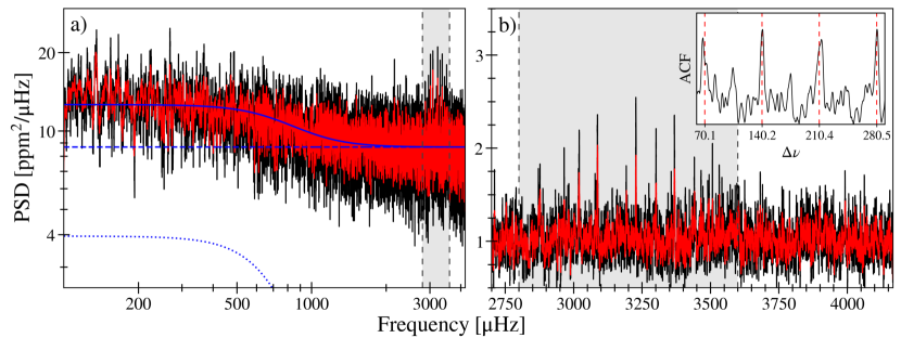
Figure 2: Panel a): Power spectrum of $\alpha$ Men A using box filters of 1.0 and 2.5 $\mu$Hz shown in black and red, respectively. The total background fit from DIAMONDS due to stellar contribution is shown by a solid blue line, which is the combination of a meso-granulation component (blue dotted line) and a white noise component (blue dashed line). Panel b): The background-corrected power spectrum is centered on the power excess due to stellar oscillations, highlighted in the shaded region. The power in this region is used to calculate an autocorrelation (ACF), shown in the inset. Dashed lines in the inset represent expected peaks in the ACF due to the characteristic spacings of p-mode oscillations.

Using the Tycho-2 $B_{T}$ and $V_{T}$ magnitudes, we derived two luminosities with isoclassify (Huber, 2017). The magnitude was combined with the Gaia parallax, bolometric corrections from MIST isochrones (Choi et al., 2016) and the composite reddening map mwdust (Bovy et al., 2016), yielding L_⋆ = 0.800 $\pm$ 0.008 L_⊙ ($B_{T}$) and L_⋆ = 0.812 $\pm$ 0.007 L_⊙ ($V_{T}$).

As an independent check on the derived luminosity, we analyzed the broadband spectral energy distribution (SED) together with the Gaia DR2 parallax following the procedures described by Stassun et al. (2017, 2018). We took the NUV flux from GALEX, the Johnson $U,B,V$ magnitudes from Mermilliod (2006), the Strömgren $u,v,b,y$ magnitudes from Paunzen (2015), the $B_{T},V_{T}$ magnitudes from Tycho-2, the $J,H,K_{S}$ magnitudes from 2MASS, the W1–W4 magnitudes from WISE, and the $G,G_{BP},G_{RP}$ magnitudes from Gaia. Together, the available photometry spans a wavelength range 0.2–22 $\mu$m.

We performed a fit using Kurucz stellar atmosphere models, adopting the effective temperature ($T_{\rm eff}$), surface gravity ($\log g$), and metallicity ([Fe/H]) from the spectroscopically determined values. The extinction ($A_{V}$) was set to zero due to the star being very nearby. The resulting fit has a reduced $\chi^{2}$ of 2.4. Integrating the (unreddened) model SED gives the bolometric flux at Earth of $F_{\rm bol}=2.494\pm 0.058\times 10^{-7}$ erg s^-1 cm^-2. Taking $F_{\rm bol}$ and $T_{\rm eff}$ together, with the Gaia parallax (adjusted by $+0.08$ mas to account for the systematic offset reported by Stassun & Torres 2018), gives the stellar radius $R=0.968\pm 0.021$ R_⊙ and bolometric luminosity $L_{\rm bol}=0.810\pm 0.019$ L_⊙. We performed an additional fit excluding the Gaia magnitudes to test if the known systematics affected the derived properties but the results were unchanged. The derived values from the SED fit are in good agreement with those derived using isoclassify.

Similar to the method discussed in Section 2.2 for the spectroscopic parameters, we performed a literature search for Gaia- and Hipparcos-derived luminosities to account for systematic differences. We used bolometric luminosities from seven independent studies (Bruntt et al., 2010; Casagrande et al., 2011; Eiroa et al., 2013; Heller et al., 2017; McDonald et al., 2017; Stevens et al., 2017; Schofield et al., 2019) along with the three luminosities derived in our study to determine the scatter in the values. We adopted the isoclassify result using the Tycho-2 $V_{T}$ magnitude and added the standard deviation of the ten values ($\sigma_{\rm{L}_{\star}}$= 0.018 L_⊙) in quadrature with our derived uncertainty ($\sigma_{\rm{L}_{\star}}$= 0.007 L_⊙) yielding a bolometric luminosity L_⋆ = 0.81 $\pm$ 0.02 L_⊙. The median value for the ten luminosities was slightly higher at L_⋆ = 0.828, but is within 1$\sigma$ of our final reported value.

3 Asteroseismology

3.1 Background Fit

A high-pass filter was applied to the TESS 2-minute light curve (Figure 1) to remove long-period trends. The power spectrum was then calculated using a Lomb-Scargle periodogram (Lomb, 1976; Scargle, 1982) through the publicly available astropy package. The power spectrum in Figure 2a shows a flat white noise component and a correlated red noise signal that rises at lower frequencies, indicative of stellar granulation. A roughly Gaussian power excess due to oscillations is clearly visible at $\sim$3200 $\mu$Hz (Figure 2b).

A common approach to model power spectra of solar-like oscillators typically has the form

$$f(\nu)=W+R(\nu)[B(\nu)+G(\nu)],$$ (1)

where $f(\nu)$ is the power density at frequency $\nu$ (Mathur et al., 2011; Corsaro et al., 2018). The frequency-independent term ($W$) is due to photon noise. The response function, $R(\nu)$, is an attenuation factor that affects the observed spectral amplitudes due to the sampling rate (or cadence) in a time series. The attenuation is greater for oscillations that occur near the Nyquist frequency, which for TESS 2-minute data is $\rm\nu_{Nyq}$ = 4166.67 $\rm\mu$Hz. The last two terms in Equation 1 refer to contributions from the stellar granulation background $B(\nu)$ and the Gaussian envelope of oscillations $G(\nu)$.

To determine the stellar background contribution, we used the publicly available Background, which is a software extension of DIAMONDS. Initially created for more robust asteroseismic analyses, DIAMONDS is a nested sampling Monte Carlo (NSMC) algorithm for Bayesian parameter estimation and model comparison (Corsaro & De Ridder, 2014). The background model built into this framework has the functional form:

$$B(\nu)=\zeta\sum_{i=1}^{n}\frac{\sigma_{i}^{2}/\nu_{i}}{1+(\nu/\nu_{i})^{4}},$$ (2)

where $\zeta$ is a normalization factor ($2\sqrt{2}/\pi$), $\sigma_{i}$ is the amplitude and $\nu_{i}$ is the characteristic frequency for $n$ Harvey-like components (Harvey, 1985). Different stellar background contributions like granulation and meso-granulation have typical characteristic frequencies of $\sim$ $\nu_{\mathrm{max}}$ and $\sim$ $\nu_{\mathrm{max}}/3$ for solar-like oscillators (Corsaro et al., 2017).

Table 3: DIAMONDS background fit using $n=1$ Harvey-like component. Values are calculated by taking the median $\pm 1\sigma$ (credible level of 68.3%) from each parameter posterior distribution.

Parameter	Value
White noise, $W$	8.67 $\pm$ 0.05 ppm2 $\mu$Hz-1
Meso-granulation timescale, $\tau_{\rm{meso}}$	20.6 $\pm$ 0.8 minutes
Meso-granulation amplitude, $\sigma_{\rm{meso}}$	59.5 $\pm$ 1.1 ppm
Gaussian height, $H_{\rm{osc}}$	0.145 $\pm$ 0.129 ppm2 $\mu$Hz-1
Gaussian center, $\nu_{\rm max}$	3134.28 $\pm$ 439.91 $\mu$Hz
Gaussian width, $\sigma_{\rm{osc}}$	403 $\pm$ 279 $\mu$Hz

We used the following configuration for the NSMC analysis: shrinking rate, $\alpha$ = 0.02; enlargement fraction, $f_{0}$ = 1.43; number of live points, $N_{\rm{live}}$ = 500; number of clusters, 3 $\leq$ $N_{\rm{clust}}$ $\leq$ 6; max attempts when drawing a new sampling point, $M_{\rm{attempts}}$ = 5$\times 10^{4}$; initial number of live points, $M_{\rm{init}}$ = $N_{\rm{live}}$; clustering only happens every N iterations or $M_{\rm{same}}$ = 50. Aside from minor changes to the shrinking rate ($\alpha$) and enlargement fraction ($f_{0}$), which control the sampling efficiency based on the number of free parameters in the model, the other parameters were the same as what was provided in the DIAMONDS documentation. We refer the reader to Corsaro & De Ridder (2014) for more details about the software.

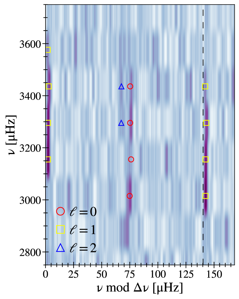
Figure 3: Échelle diagram of $\alpha$ Men A from a smoothed power spectrum (with a boxcar filter width of 2.5 $\mu$Hz) using. echelle (Hey & Ball, 2020). Different oscillation modes are marked and colored by their spherical degree: radial modes ($\ell=0$) by red circles, dipole modes ($\ell=1$) by yellow squares, and quadrupole modes ($\ell=2$) by blue triangles. The large frequency separation derived from radial modes is $\Delta\nu$ = $140.24\pm 1.98$ $\mu$Hz and is delineated by the black dashed line.

Ultimately, the data did not provide enough evidence for DIAMONDS to converge on reliable results for more complex models (i.e. multiple Harvey-like terms), and therefore no model comparison was needed. We attempted to model the granulation component but it was mostly unconstrained or resulted in very small amplitudes. This is likely because the amplitude of the granulation signal is comparable to or less than the white noise level in the power spectrum. The final background fit is shown in Figure 2a as a solid blue line, which is the summed contributions from a white noise component (blue dashed line) and a meso-granulation term (blue dotted line).

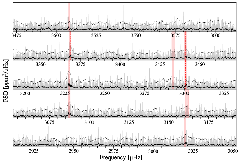
Figure 4: Power spectrum of $\alpha$ Men A arranged in échelle format. The original power spectrum calculated using TESS data (Section 2.1) is shown in grey, as well as a smoothed version of the same power spectrum (using a boxcar width = 1.5 $\mu$Hz) in black. The weighted power spectrum discussed in Section 3.4 is overplotted by a dotted black line with a vertical offset for a direct comparison. The final frequencies from Table 4 are added in red, where shaded regions are equal to $\pm 1\sigma$ for each mode.

3.2 Global Asteroseismic Parameters

The shaded region in Figure 2b shows the power excess due to oscillations. Within the DIAMONDS framework, this power excess is modeled by a Gaussian

$$G(\nu)=H_{\rm{osc}}\,\rm{exp}\bigg{[}-\frac{(\nu-\nu_{\rm{max}})^{2}}{2\sigma_{\rm{osc}}^{2}}\bigg{]},$$ (3)

centered at $\nu_{\rm max}$with height $H_{\rm{osc}}$ and width $\sigma_{\rm{osc}}$ (Corsaro & De Ridder, 2014). The resulting parameters of the global DIAMONDS analysis for $\alpha$ Men A are listed in Table 3.

We also derived an independent value for the frequency corresponding to maximum power using the SYD pipeline (Huber et al., 2009), yielding $\nu_{\rm max}$ $\sim 3267$ $\mu$Hz, consistent with the results from DIAMONDS. Two independent analyses additionally confirmed power excess in the same region, with $\nu_{\rm max}$ = 3230 $\mu$Hz (A2Z; Mathur et al., 2010) and $\nu_{\rm max}$ = 3216 $\mu$Hz (Lundkvist, 2015), both consistent to $\lesssim\,$1$\sigma$ from our derived values. Our derived $\nu_{\rm max}$ is larger than that in the Sun ($\nu_{\rm{max},\odot}$ = 3090 $\mu$Hz). Therefore, $\alpha$ Men A joins only a handful of other stars such as $\tau$ Cet (Teixeira et al., 2009), $\alpha$ Cen B (Carrier & Bourban, 2003; Kjeldsen et al., 2005) and Kepler-444 (Campante et al., 2015) that have a higher $\nu_{\rm max}$ than the Sun.

To estimate a preliminary value for the large frequency separation, we calculated an échelle diagram. In the case of solar-like oscillators, modes of different radial order ($n$) with the same spherical degree ($\ell$) should form vertical ridges if the correct spacing is used. We calculated the best-fitting value by taking small steps in frequency space until the ridges lined up vertically, yielding $\Delta\nu$ $\sim$140 $\mu$Hz. Figure 4 shows the resulting échelle diagram created using echelle (Hey & Ball, 2020), which clearly confirms the detection of solar-like oscillations.

3.3 Individual Frequencies

We extracted frequencies from the background-corrected power spectrum using three independent methods, which are based on fitting Lorentzian profiles to individual modes (GarcÍa et al., 2001; García et al., 2009; Handberg & Campante, 2011; Nielsen et al., 2015, 2017). A second approach used an alternative power spectrum calculated using weights to account for different noise levels across time series (Arentoft et al., 2008).

To compare the two approaches, Figure 4 shows both the unweighted (solid grey/original, black lines/smoothed) and weighted (dotted black line) power spectrum stacked by radial order $n$ about $\nu_{\rm max}$. The figure clearly exhibits the consistency between the two independently-calculated spectra, especially for the higher signal-to-noise (SNR) modes.

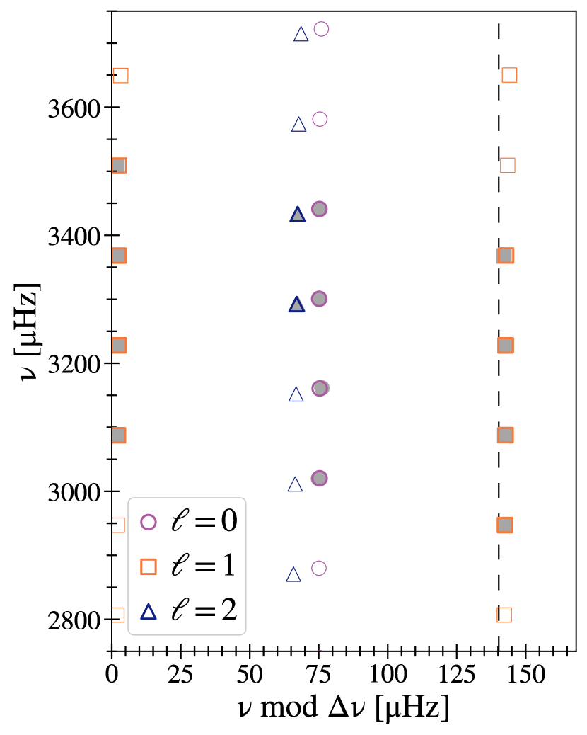
Figure 5: Échelle diagram of observed frequencies (filled gray symbols) and best-fit model frequencies (open colored symbols) using BeSPP (Serenelli et al., 2013, 2017). Modeled frequencies that correspond to an observed frequency are highlighted with a thicker marker outline.

Our final frequency list was constructed by taking modes for which both approaches reported a detection. We report 4 radial ($\ell=0$) modes, 4 dipole ($\ell=1$) modes, and 2 quadrupole ($\ell=2$) modes in Table 4. Formal uncertainties were adopted using the frequencies calculated from the weighted power spectrum and adding in quadrature the scatter in frequencies derived from independent methods to account for systemic uncertainties. The final set of frequencies are plotted on the échelle diagram (Figure 3, marked by their spherical degree $\ell$) and on the stacked power spectrum (Figure 4).

3.4 Frequency Modeling

To properly account for systematic uncertainties, we derived fundamental stellar properties of $\alpha$ Men A using nine independent modeling pipelines, including BASTA (Silva Aguirre et al., 2015), YB (Basu et al., 2010; Gai et al., 2011; Basu et al., 2012), AMP (Metcalfe & Charbonneau, 2003; Metcalfe et al., 2009a, 2012a), BeSPP (Serenelli et al., 2013, 2017), Izmir (Yıldız et al., 2019), GOE (Silva Aguirre et al., 2017) and YALE-M (Tasoulis et al., 2004; Mier, 2017; Ball et al., 2020). Model grids were calculated from various stellar evolution codes (YY, Demarque et al. 2004; MESA r10398, r12115, r15140, Paxton et al. 2011, 2013, 2015, 2018, 2019; GARSTEC, Weiss & Schlattl 2008; YREC, Demarque et al. 2008; BaSTI, Pietrinferni et al. 2004; DSEP, Dotter et al. 2007, 2008; CESAM2k, Morel & Lebreton 2008; YREC2, Basu et al. 2012; ASTEC, Christensen-Dalsgaard 2008; CESTAM, Marques et al. 2013; and Padova, Marigo et al. 2008; Girardi et al. 2000) using different assumptions about input physics. Oscillation frequencies were generated from oscillation codes (ADIPLS, Christensen-Dalsgaard 2008; GYRE, Townsend & Teitler 2013), where most of the methods listed here also applied corrections for near-surface effects (Kjeldsen et al., 2008; Ball & Gizon, 2014).

Table 4: Extracted mode identifications and oscillation frequencies for $\alpha$ Men A sorted by spherical degree $\ell$.

$\nu$ ($\mu$Hz)	$\sigma_{\nu}$ ($\mu$Hz)	$n$	$\ell$
3019.95	0.50	23	0
3161.43	0.99	24	0
3300.84	0.69	25	0
3441.14	0.87	26	0
3087.44	0.59	23	1
3227.69	0.52	24	1
3368.55	0.44	25	1
3507.88	0.58	26	1
3292.93	0.47	24	2
3433.30	0.95	25	2

Each method derived four sets of stellar parameters based on the following sets of constraints:

1. {$T_{\mathrm{eff}}$, [Fe/H], $L_{\star}$, $\nu_{\rm max}$, $\Delta\nu$, $\nu(n,0)$, $\nu(n,1)$, $\nu(n,2)$}

2. {$T_{\mathrm{eff}}$, [Fe/H], $\nu_{\rm max}$, $\Delta\nu$, $\nu(n,0)$, $\nu(n,1)$, $\nu(n,2)$}

3. {$T_{\mathrm{eff}}$, [Fe/H], $L_{\star}$, $\nu_{\rm max}$, $\Delta\nu$, $\nu(n,0)$, $\nu(n,1)$}

4. {$T_{\mathrm{eff}}$, [Fe/H], $\nu_{\rm max}$, $\Delta\nu$, $\nu(n,0)$, $\nu(n,1)$}

The main purpose for all four runs was to test for inconsistencies between the luminosity derived from asteroseismology and the independent $Gaia$-derived luminosity, as well as to check if the weaker quadrupole ($\ell=2$) modes had any affect on the final age estimates. Results from each pipeline were self-consistent in that the runs that excluded the quadrupole modes generally preferred younger ages but ultimately the differences were not significant ($\leq$10%) and $\lesssim$1$\sigma$. Moreover, across the numerous methods and model inputs mentioned, the derived stellar parameters between all pipelines agreed to within 1$\sigma$.

For final stellar parameters, we adopted the results from BeSPP (Bellaterra Stellar Properties Pipeline, Serenelli et al., 2013, 2017), which was closest to the median values for fundamental stellar parameters (mass and age) in case 1. BeSPP constructed a grid of stellar models with GARSTEC (Weiss & Schlattl, 2008) using a gray model atmosphere based Vernazza et al. (1981), the solar mixture model from Grevesse & Noels (1993), and the diffusion of elements according to Thoul et al. (1994). We refer the reader to Weiss & Schlattl (2008) for more details on the input physics of stellar models computed with GARSTEC. BeSPP yielded a bimodal solution as a result of a bimodal surface correction, which at a fixed mass, was older ($\sim$2 Gyr) and more metal rich ($\sim$0.1 dex). The surface correction for the younger solution was unexpectedly large ($\sim$50$\mu$Hz) for a solar analogue and hence provided strong support in favor of the older model.

To account for systematic differences between various methods, uncertainties were calculated by adding the standard deviation for each parameter {$M$, $R$, $\rho$, $\tau$, $\log g$} from all pipelines in quadrature with the formal uncertainty from BeSPP. Corrected model frequencies are plotted with the observed frequencies in an échelle diagram in Figure 5. Stellar parameters are listed in Table 2 (i.e. see the asteroseismology section), with fractional uncertainties of 1.4% (1.2% stat $\pm$ 0.7% sys) in density, 1.7% (1.4% stat $\pm$ 0.9% sys) in radius, 4.7% (3.9% stat $\pm$ 2.7% sys) in mass, and 24.2% (21.8% stat $\pm$ 10.4% sys) in age.

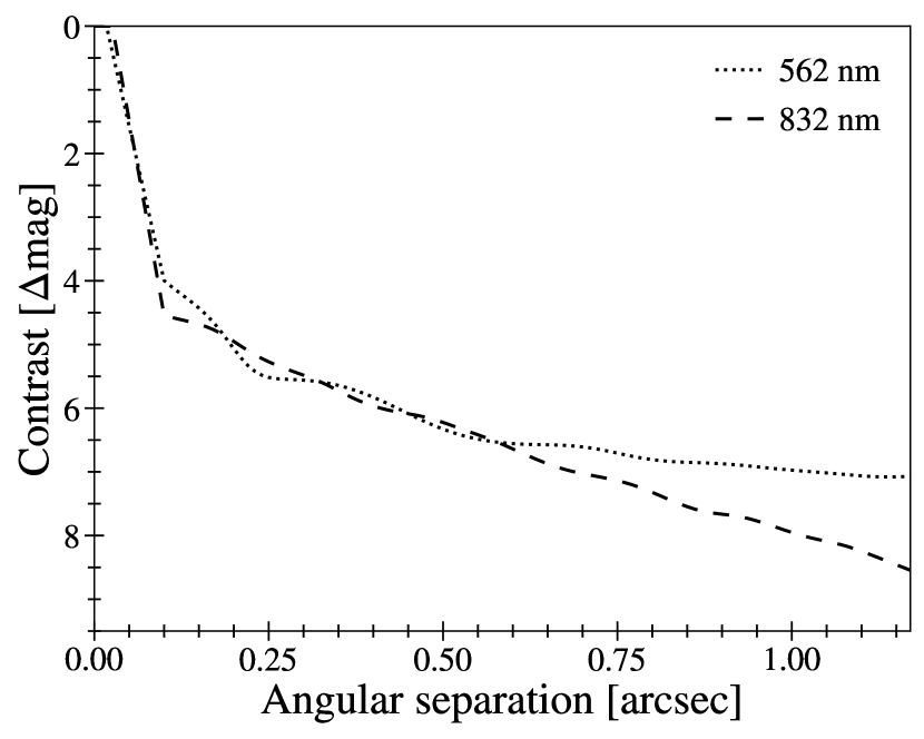
Figure 6: Detection limits from speckle imager Zorro on the Gemini South telescope in r- and z-band (562 nm and 832 nm, respectively), ruling out any additional close-in companions to the contrast levels obtained.

Table 5: Secondary Stellar Parameters

Other identifiers:
$\alpha$ Men B, HD 43834 B
Gaia DR2/eDR3 5264749303457104384
Parameter	Value	Method
Gaia1,2
Right ascension (RA), $\rm\alpha_{J2016}$	$92.5590$	A
Declination (Dec), $\rm\delta_{J2016}$	$-74.7542$	A
Parallax, $\pi$ (mas)	$97.8666\pm 0.0898$	A
Distance, $d$ (pc)	$10.2180\pm 0.0094$	A
Gaia G mag, $G$	$12.3653\pm 0.0044$	P
Gaia G contrast, $\Delta G$	$7.4652\pm 0.0053$	P
Other Work3,4,5
Projected separation, $\rm\rho_{K}$ (′′)	3.02 $\pm$ 0.01	A
Position angle, $\rm PA_{K}$ (o)	250.87 $\pm$ 0.11	A
NACO K contrast, $\rm\Delta m_{K}$	4.97 $\pm$ 0.05	P
2MASS KS mag, $\rm K_{S}^{*}$	$8.476\pm 0.200$	P
Spectral type	M3.5–M6.5	R1
Stellar mass, $M_{\star}$ ($M_{\odot}$)	0.14 $\pm$ 0.01	R2
Orbital period, $P$ (years)	162.04	-
This Work
Effective temperature, $T_{\mathrm{eff}}$ (K)	$3054\pm 44$	E
Stellar radius, $R_{\star}$ ($R_{\odot}$)	$0.19\pm 0.01$	E
Stellar mass, $M_{\star}$ ($M_{\odot}$)	$0.169\pm 0.006$	E
Age, $t$ (Gyr)	$6.2\pm 1.4$	F
Orbital period, $P$ (years)	157.44	-

References – (1) Gaia Collaboration et al. (2016) (2) Gaia Collaboration et al. (2021) (3) Eggenberger et al. (2007) (4) Cutri et al. (2012) (5) Tokovinin (2014)

Methods – (A) Astrometry, (E) empirical relations derived from Mann et al. (2015) and Mann et al. (2019), (R1) relationship between absolute magnitude and spectral type from Eggenberger et al. (2007) (using data from Delfosse et al. (2000), Leggett et al. (2001), Dahn et al. (2002), and Vrba et al. (2004)) (R2) infrared mass-luminosity relation for low-mass stars (Delfosse et al., 2000), (P) photometry, or (F) frequency modeling via asteroseismology.

Notes –
^∗ The provided Ks magnitude uncertainty for the companion was less than that reported by Cutri et al. (2012) for the primary. Therefore, we inflated the uncertainty in the Ks magnitude for HD 43834 B to reflect that.

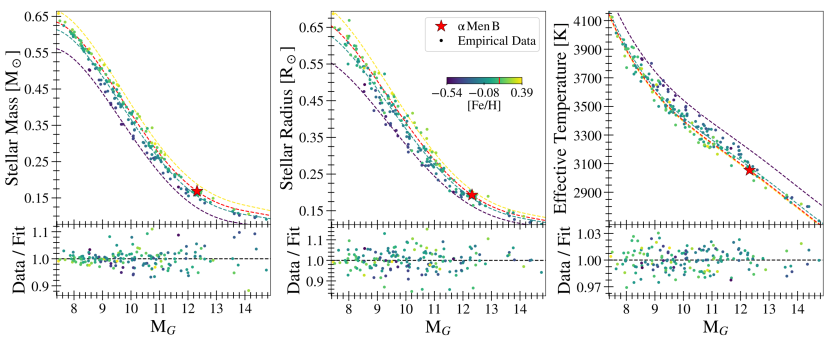
Figure 7: Empirical best-fit relations for mass (left), radius (middle) and temperature (right) as a function of absolute Gaia magnitude for the sample in Mann et al. (2015) color-coded by metallicity. The bottom plot shows the residuals of the data subtracted by the best fit polynomial (black dashed line). The red star represents the location of $\alpha$ Men B.

4 M-dwarf Companion

4.1 Discovery & Initial Characterization

A bound M-dwarf companion to $\alpha$ Men A was first identified by Eggenberger et al. (2007) in a study investigating the impact of stellar duplicity on planet occurrence rates using adaptive optics imaging with NACO/VLT. Eggenberger et al. (2007) ruled out the possibility of HD 43834 B being a background star, stating that the astrometry was compatible with orbital motion. In addition, they added that the physical association was further supported by a linear drift present in CORALIE data.

Eggenberger et al. (2007) reported a magnitude difference of $\Delta$m = 4.97 $\pm$ 0.05 in the narrowband K filter ($\lambda_{c}=2.166\,\mu$m). After a correction to account for the differences in relative photometric systems, they reported an absolute 2MASS Ks magnitude, M${}_{K_{\rm s}}$ = 8.43 $\pm$ 0.05 for the companion. They concluded that HD 43834 B is consistent with an M3.5-M6.5 dwarf companion with a mass of M_⋆,B = 0.14 $\pm$ 0.01 $M_{\odot}$ at a projected separation of 3” from the primary, which corresponds to a physical separation of $\sim$30 AU. Tokovinin (2014) characterized nearby multiple star systems and, using the literature mass of M_⋆,A = 1.01 $M_{\odot}$for the primary, estimated an orbital period of $\sim$162 years for the wide companion.

4.2 A Search for Additional Companions

To search for additional close companions, we observed $\alpha$ Mensae with Zorro, a dual-channel imager on the 8.1-m telescope at the Gemini South Observatory (Cerro Pachon, Chile). Zorro provides simultaneous diffraction-limited optical imaging (FWHM 0.02” at 650nm) in 2 channels. We observed $\alpha$ Men A in speckle mode to search for close-in companions between UT December 22 2019 and December 23 2019. The images were subjected to the standard Fourier analysis as described in Howell et al. (2011) and were used to produce reconstructed images in each color providing high-resolution angular results. In addition to detecting the M dwarf companion at 3” distance, no other companions to Mensae were found. Figure 6 shows the contrast curves from the reduced speckle data in both bands, indicating that there are no additional close companions ($<$1.2”) from the diffraction limits down to contrasts of $\Delta\mathrm{m}\sim 7$ in r-band (562 nm) and $\Delta\mathrm{m}\sim 8$ in z-band (832 nm). At the distance of $\alpha$ Mensae, these angular limits correspond to spatial limits of 0.2 to 1.2 AU.

4.3 Revised Properties of $\alpha$ Men B

The wide companion was resolved in Gaia DR2, which reported a magnitude of $G=11.8057$ and a contrast of $\Delta G=6.955$. However, the early Gaia Data Release 3 (eDR3; Gaia Collaboration et al., 2021; Riello et al., 2021) reported a significantly fainter companion with $G$ = 12.365, corresponding to a contrast of $\Delta G$ = 7.465. Additionally, eDR3 provided a parallax for the companion, which was unavailable in DR2.

In order to estimate the companion properties, we derived empirical relations for masses, effective temperatures, and radii of M dwarfs given the absolute Gaia magnitude ($\mathrm{M}_{G}$). We adopted the $T_{\mathrm{eff}}$ and radius values from Mann et al. (2015) and used the $\mathrm{M}_{K}$-mass relation from Mann et al. (2019) to estimate the M-dwarf masses. We computed the absolute Gaia magnitudes using eDR3 (Gaia Collaboration et al., 2021) photometry (Riello et al., 2021) and parallaxes (Lindegren et al., 2021), including the relevant corrections when applicable. We removed two stars from the Mann et al. (2015) sample for our relations: Gl 896 B, due to its largely discrepant measurements in mass, $T_{\mathrm{eff}}$, and radius, and FBS L 10-72 due to its discrepant [Fe/H] given its other measured values. For each of the three parameters ($T_{\mathrm{eff}}$, $R_{\star}$, $M_{\star}$), we optimized polynomial coefficients using a least-squares minimization method available with scipy. Finally, to select the optimal order, we chose the curve that minimized the Bayesian Information Criterion (BIC; Schwarz, 1978).

Figure 7 shows the resulting relations, which are:

$$\begin{split}\mathrm{M}_{\star}=-7.0653+3.0293x-0.4218x^{2}\\ +0.0244x^{3}-0.0005x^{4}+0.1771y-0.0087xy,\end{split}$$ (4)

$$\begin{split}T_{\mathrm{eff}}=19938.4-4999.7x+582.0x^{2}\\ -30.8x^{3}+0.6x^{4}-131.0y+208.0y^{2},\end{split}$$ (5)

and

$$\begin{split}\mathrm{R}_{\star}=(-4.1305+1.9735x-0.2832x^{2}\\ +0.0166x^{3}-0.0003x^{4})\times(1+0.2450y),\end{split}$$ (6)

where $x$ is the absolute Gaia magnitude $\rm M_{\mathit{G}}$ from eDR3 and $y$ is the metallicity from Mann et al. (2015).

Using the Gaia absolute magnitude for $\alpha$ Men B and metallicity for $\alpha$ Men A, the relations yield a mass of $M_{\star}$ = $0.169\pm 0.006$ $M_{\odot}$, radius of $R_{\star}$ = $0.19\pm 0.01$ $R_{\odot}$ and $T_{\mathrm{eff}}$ = $3054\pm 44$ K for $\alpha$ Men B. Uncertainties were calculated from the residual scatter between the models and data, which are 3.7% in mass, 4.4% in radius and 44 K in $T_{\mathrm{eff}}$. The mass uncertainty was calculated using the scatter of 2.2% in our derived relation (Equation 4) added in quadrature with the conservative estimate of 3% from the Mann et al. (2019) $\mathrm{M}_{Ks}-\mathrm{M}_{\star}$ relation. Notably, our derived mass of $0.169\pm 0.006$ $M_{\odot}$ for the fully-convective M dwarf is slightly higher than the value of 0.14 $\pm$ 0.01 $M_{\odot}$ from Eggenberger et al. (2007), which was based on an infrared mass-luminosity relation for low-mass stars. All observed and derived properties of $\alpha$ Men B are summarized in Table 5.

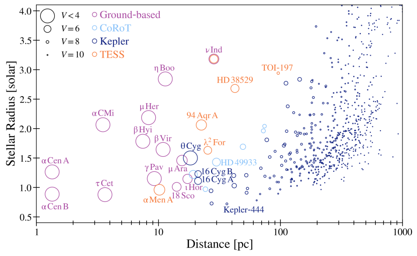
Figure 8: Current population of asteroseismic detections with confirmed $\Delta\nu$ measurements plotted as the stellar size (in solar radii) as a function of distance, where markers are sized by their visual magnitude. Ground-based seismic detections (purple) are limited to close, bright stars while Kepler (navy blue) found hundreds of oscillations in faint, distant stars. TESS (orange) is beginning to close the gap between these two regimes and hence, providing bright nearby targets to follow up with ground-based instruments. In fact, $\nu$ Ind is the first example where an early ground-based asteroseismic detection (Bedding et al., 2006) was redetected later with TESS (Chaplin et al., 2020). Label references (in order of proximity) – $\alpha$ Cen A (Brown et al., 1991; Bouchy & Carrier, 2001, 2002; Butler et al., 2004; Bedding et al., 2004), $\alpha$ Cen B (Carrier & Bourban, 2003; Kjeldsen et al., 2005), $\alpha$ CMi (Mosser et al., 1998; Martić et al., 1999; Arentoft et al., 2008; Bedding et al., 2010), $\tau$ Cet (Teixeira et al., 2009), $\beta$ Hyi (Bedding et al., 2001; Carrier et al., 2001; Bedding et al., 2006), $\mu$ Her (Bonanno et al., 2008; Grundahl et al., 2017), $\gamma$ Pav (Mosser et al., 2008), $\alpha$ Men A (this work), $\beta$ Vir (Carrier et al., 2005b), $\eta$ Boo (Kjeldsen & Bedding, 1995; Kjeldsen et al., 2003; Carrier et al., 2005a), 18 Sco (Bazot et al., 2011), $\mu$ Ara (Bouchy et al., 2005), $\iota$ Hor (Vauclair et al., 2008), $\theta$ Cyg (Guzik et al., 2011), 16 Cyg A & B (Metcalfe et al., 2012b), 94 Aqr A (Metcalfe et al., 2020), $\lambda^{2}$ For (Nielsen et al., 2020), $\nu$ Ind (Bedding et al., 2006; Carrier et al., 2007; Chaplin et al., 2020), $\rm HD\,49933$ (Appourchaux et al., 2008; Benomar et al., 2009), Kepler-444 (Campante et al., 2015), $\rm HD\,38529$ (Ball et al., 2020), and TOI-197 (Huber et al., 2019).

5 Discussion

5.1 Testing Stellar Physics with Asteroseismology

Asteroseismology of nearby bright stars allows us to test stellar models by combining with other high-resolution stellar classification techniques like spectroscopy, interferometry, and astrometry (Bruntt et al., 2010; Silva Aguirre et al., 2012; Hawkins et al., 2016). An example is Bruntt et al. (2010), who combined interferometry, asteroseismology, and spectroscopy to derive the most accurate and precise fundamental properties for 23 bright stars.

Figure 8 shows radii and distances of stars in which solar-like oscillations have been studied. The brightest detections were discovered prior to the launches of Kepler and CoRoT (Convection Rotation and planetary Transits; Baglin et al., 2006). This means that most bright stars only have asteroseismology from ground-based radial velocity measurements, which suffer from aliasing problems due to gaps in data. Examples of well-known ground-based asteroseismic detections include $\beta$ Hyi (Bedding et al., 2001; Carrier et al., 2001; Bedding et al., 2006), $\alpha$ Cen A (Bouchy & Carrier, 2002; Bedding et al., 2004), and $\alpha$ Cen B (Carrier & Bourban, 2003; Kjeldsen et al., 2005).

The flood of continuous high-precision high-cadence photometry from CoRoT and Kepler marked the start of the so-called “space-based photometry revolution”. Kepler revolutionized the field of asteroseismology by detecting oscillations in $\sim$500 main-sequence and subgiant stars. However, most Kepler targets are faint and distant, and thus do not have information from complementary techniques such as interferometry. This limitation was only partially solved by novel techniques called “halo” and “smear” photometry, which allowed the production of high-precision light curves for even heavily saturated Kepler stars (Pope et al., 2016; White et al., 2017; Pope et al., 2019a, b).

The TESS mission provides an ideal solution to this problem. Several early asteroseismic detections by TESS have been made for bright nearby stars such as $\nu$ Ind (Chaplin et al., 2020), HD 38529 (Ball et al., 2020), $\lambda^{2}$ For (Nielsen et al., 2020), 94 Aqr A (Metcalfe et al., 2020), and the first new TESS asteroseismic host, TOI-197 (Huber et al., 2019). Alpha Men A is now the closest solar analogue with an asteroseismic detection from space, making it a prime example of a bright benchmark system from the nominal TESS mission. In fact, $\alpha$ Men A was included in Bruntt et al. (2010), but was the only star in the sample without an asteroseismic detection.

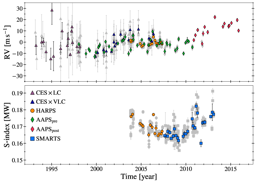
Figure 9: Long-term ground-based RV (top) and Mount Wilson calibrated S-index (bottom) time series for $\alpha$ Men A using combined data from 5 different surveys. Each instrument is shown by a different marker, where offsets and/or upgrades of a similar instrument are shown by a different color. Grey points are original data from each survey and colored points are binned over 60 days. We find a long-term cyclic trend of $\sim$13 years in both RVs and chromospheric emission, indicative of a stellar activity cycle.

5.2 Stellar Activity

The connection between oscillations and activity cycles are important to understand the long-term magnetic evolution of stars. For example, observations in the Sun have shown a strong correlation between oscillation frequencies and amplitudes with the solar activity cycle (Broomhall et al., 2011). Currently there are only a handful of examples that exist for stars other than the Sun (e.g. García et al., 2010), and therefore expanding this sample to more stars would be very valuable. Fortunately TESS is already well-positioned for this, as demonstrated by Metcalfe et al. (2020) who combined TESS asteroseismology with 35 years of activity measurements to study the evolution of rotation and magnetic activity in 94 Aqr Aa.

Stellar activity is traditionally observed indirectly through long-term monitoring of chromospheric emission in the Ca ii H and K lines (Noyes et al., 1984; Baliunas et al., 1995; Henry et al., 1996). More recently, Santos et al. (2010) and Lovis et al. (2011) used RVs derived from the cross-correlation function (CCF) method to show that stellar activity also correlates with parameters from the CCF like the FWHM and the bisector inverse slope (BIS). Indeed a study by Zechmeister et al. (2013) compared archival HARPS RVs with three different indicators for $\sim$30 well-studied stars and found a positive correlation with all three ($\log R^{\prime}_{\rm{HK}}$, BIS, FWHM) for alpha Men, indicative of a magnetic cycle as a cause of the RV variations. However, the main goal of the study was to observationally confirm the existence of correlations in RV indicators and they did not report any activity cycle periods.

To investigate the stellar activity cycle for $\alpha$ Men A, we collected publicly available RV data from two instruments on the ESO 3.6m telescope: the Coudé Echelle Spectrograph (CES, pre- and post-upgrade) and HARPS, which was already corrected for systemic instrumental offsets in Zechmeister et al. (2013). We also collected data from the Anglo-Australian Planet Search (AAPS), which perfectly overlapped with the CES and HARPS data. Figure 9 shows the complete RV time series, which covers 22 years. AAPS data after 2011 is plotted as a separate instrument because of an unexplained RV offset. We used a conservative bin size of 60 days to average over the scatter due to stellar rotation, revealing a period which is similar to that observed in the Sun. Using the publicly available GLS code (Zechmeister & Kürster, 2009), a generalized Lomb-Scargle periodogram analysis that is better suited for unevenly (and sparsely) sampled data, we detect a period $P=$ 13.1 $\pm$ 1.1 years in the RV time series. There is evidence for a long-term linear trend which is likely from the companion, depending on the inclination of the system. Note that we did not correct for any additional systematic offsets when we combined the time series from multiple instruments.

To confirm that the RV variations are due to an activity cycle, we analyzed the Mount Wilson calibrated S-index time series available from the HARPS DRS pipeline. Chromospheric emission in alpha Men was also observed as part of the SMARTS southern HK project from 2007-2013 (Metcalfe et al., 2009b). The bottom of Figure 9 shows the combined S-index time series, which span roughly one activity cycle and follow a similar trend to that seen in the RVs. This suggests that the observed RV variations are intrinsic to the star and not from a long-period planetary mass companion, providing additional evidence in support of an activity cycle detection.

5.3 Gyrochronology

Recent observations of stellar rotation periods have challenged commonly adopted age-rotation relationships in two distinct parameter spaces. Specifically, the observation of slow rotation periods in middle-aged solar-type stars has been proposed to be related to weakened magnetic braking due to stellar winds (van Saders et al., 2016), while the stalled spin-down observed in lower mass cluster members (Curtis et al., 2019) has been hypothesized to be related to reduced angular momentum transport caused by a decoupling of the convective core and the radiative envelope (Spada & Lanzafame, 2020). At an age of $\sim$6 Gyr, $\alpha$ Men A is in the latter half of its main sequence life and therefore provides a valuable test for the weakened braking hypothesis. Alpha Men B, on the other hand, is a fully convective M dwarf and thus provides an excellent test of whether core-envelope decoupling is indeed responsible for the stalled spin-down in M dwarfs with radiative envelopes. Consequently, rotation periods for either star in the $\alpha$ Mensae system would be extremely valuable to calibrate gyrochronology, which is currently the most promising method for ages for field dwarfs.

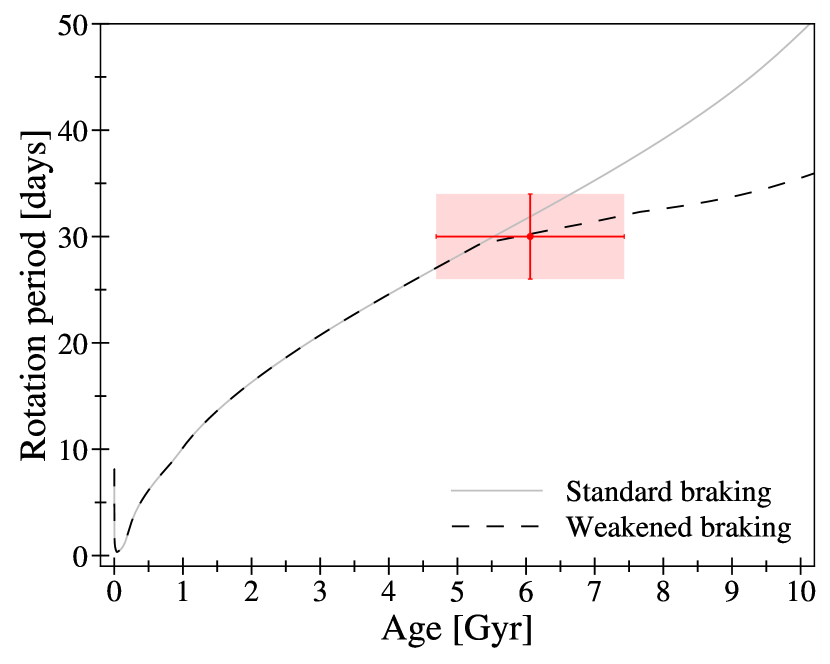
Figure 10: Predicted rotation periods of $\alpha$ Men A from gyrochronology models using a standard braking law (solid grey line, van Saders & Pinsonneault, 2013) and a weakened braking law (dashed black line, van Saders et al., 2016). The rotation period uncertainties were calculated by taking the average of the lower and upper quantiles from the corner plots derived by kiauhoku (Claytor et al., 2020), where the more conservative uncertainty of 4.5 days is plotted in this figure. The shaded red area represents the 1$\sigma$ uncertainty region for the location of $\alpha$ Men A with respect to theoretical gyrochronological models, which predicts that the solar analogue has recently undergone or is currently in transition in its rotational behavior.

Saar & Osten (1997) reported a rotation period ($P_{\rm{rot}}$) of 32 days for alpha Men based on Ca ii flux measurements. Futher investigation showed that the rotation period was not directly observed but empirically derived. A relationship between chromospheric activity and the Rossby number (Ro) of a star, a parametrization of the rotation period and convective turnover time ($\tau_{\rm{conv}}$), was established by Noyes et al. (1984) and updated by Mamajek & Hillenbrand (2008) using a larger sample of stars. For $\alpha$ Men A, a mean activity level log$R^{\prime}_{\rm{HK}}$ = -4.94 from Henry et al. (1996) with Eq.5 (Mamajek & Hillenbrand, 2008) yields Ro = 2.05. Using Eq.4 from Noyes et al. (1984) and the Johnson color index $(B-V)_{J}$ = 0.72 for the primary, estimate a turnover time of log$\,\tau_{c}$ = 1.192. We arrive at an approximate value of $P_{\rm{rot}}$ $\sim$32 days, in agreement with the value reported by Saar & Osten (1997).

We also calculated the color index from the Tycho-2 catalog (Høg et al., 2000) using the transformation from B_T and V_T to Johnson indices (see Section 1.3 Appendex 4 from Hipparcos catalog, ESA 1997). We used this color index $(B-V)_{J}$ = 0.69 to obtain log$\,\tau_{c}$ = 1.16 and $P_{\rm{rot}}$ $\sim$30 days. It is also worth pointing out that the updated empirical age-activity-rotation relation from Mamajek & Hillenbrand (2008) estimated an age of 5.5 Gyr for $\alpha$ Men, which is consistent with our asteroseismic age.

To search for stellar rotational modulation we analyzed the TESS SAP light curve, which is more conservative in preserving long-term variability than the PDCSAP light curve shown in Figure 1. We identified a period around 36 days, consistent with the estimates from activity indicators. We caution however that this period is highly uncertain due to intra-sector TESS systematics, which are non-negligible and therefore make it difficult to detect reliable rotation periods $\gtrsim$13 days.

Using the asteroseismic age, we calculated rotation periods of $\alpha$ Men A using different spindown models. Figure 10 shows the rotation period for the primary as a function of age using YREC (Yale Rotating stellar Evolution Code; Demarque et al., 2008) models with a standard braking law (van Saders & Pinsonneault, 2013) and a stalled braking law (van Saders et al., 2016), as implemented in kiauhoku (Claytor et al., 2020). The models predict rotation periods of 30.4 $\pm$ 4.5 days and 29.6 $\pm$ 3.0 days respectively, indicating that alpha Men A may be close to the critical Rossby number, which is suggested to mark a transition in its rotational behavior (Metcalfe et al., 2016), leading to a weakened spindown (van Saders et al., 2016).

Gyrochronology of M dwarfs remains challenging, mostly because the required constraints (e.g. $P_{\mathrm{rot}}$, ages) are not readily available. In particular, $\alpha$ Men B is below the convective boundary, where braking laws are uncertain. While the rotation period for the M dwarf is currently unknown, measuring a period in combination with the asteroseismic age would be valuable to place better constraints on gyrochronology models in low-mass stars.

5.4 Exoplanet Synergies

The future of exoplanet characterization will be heavily focused on direct imaging, which provides direct information about the planet composition and atmosphere. The next generation of space-based imaging missions (e.g., LUVOIR The LUVOIR Team 2019; HabEx, Gaudi et al. 2020) will be equipped with instruments capable of imaging Earth-like planets around nearby stars.

A critical challenge for future direct imaging missions will be target selection. Historically, lower luminosity M-dwarfs have been popular targets when searching for rocky potentially habitable planets, since the habitable zones (HZs) are close to the host star. While this is ideal for methods such as transits and RVs that yield larger signals for planets that are closer in, the smaller separation is challenging for direct imaging. Consequently, the prime targets for missions like LUVOIR and HabEx will be nearby, well-characterized Sun-like stars, whose HZ is further from the host star. Bixel & Apai (2020) discussed the importance of age-based target selection specifically in the context of understanding planet habitability, noting that the presence of oxygen in the Earth’s atmosphere has had a rich dynamic history. An Earth analogue around $\alpha$ Men A has a predicted separation of $\sim$100 mas and contrast $\sim 5\times 10^{-9}$, in reach for next-generation space-based imaging missions.

Additionally, new spectrographs have recently achieved the sub-meter-per-second precision that is needed to detect an Earth-like planet around a Sun-like star through precise radial velocities (PRVs). A major limitation for these efforts has been the background from stellar signals that have comparable periods and amplitudes to low-mass planetary companions, which can lead to spurious detections. Several newer techniques have been developed to help mitigate the effects induced on PRVs as a result of stellar activity (e.g. Damasso & Del Sordo, 2017; Feng et al., 2017; Dumusque, 2018; Zhao & Tinney, 2020). Our newly reported activity cycle for $\alpha$ Men A (P = 13.1 +/- 1.1 years with an amplitude of $\sim$5.5 $\rm m\,s^{-1}$) is consistent with the long-term RV scatter found in Wittenmyer et al. (2016)) and could potentially help disentangle smaller planet-like signals with ground-based PRV surveys.

6 Conclusions

We have used asteroseismology to precisely characterize the solar-analogue $\alpha$ Men A and its M-dwarf companion. Our main conclusions can be summarized as follows:

• Alpha Men A is a naked-eye G7 dwarf in TESS’s Southern Continuous Viewing Zone. Combined astrometric, spectroscopic and asteroseismic modeling confirmed the solar-analogue nature, with $R_{\star}$ = 0.960 $\pm$ 0.016 $R_{\odot}$, $M_{\star}$ = 0.961 $\pm$ 0.045 $M_{\odot}$, and an age of 6.1 $\pm$ 1.4 Gyr. Alpha Men A is the closest star cooler than the Sun with an asteroseismic detection from space-based photometry and demonstrates the power of TESS for cool dwarf asteroseismology.

• Alpha Men A has a bound companion, which was previously characterized as a mid-to-late M dwarf using 2MASS photometry. Using Gaia eDR3 photometry, we derived empirical M-dwarf relations for mass, effective temperature and radius as a function of metallicity. Using the relations, we provide revised properties of the fully-convective late M dwarf ($R_{\star}$ = $0.19\pm 0.01$ $R_{\odot}$, $M_{\star}$ = $0.169\pm 0.006$ $M_{\odot}$, $T_{\mathrm{eff}}$ = $3054\pm 44$ K). Through the asteroseismic characterization of the primary, Alpha Men B joins a very small population of M dwarfs with a precisely measured age.

• We used a combination of multiple radial velocity surveys to measure an activity cycle of P = 13.1 $\pm$ 1.1 years in $\alpha$ Men A, making it a prime target to investigate the interplay of long-term magnetic evolution and stellar oscillations in a solar-type star.

• Using the asteroseismic age, we used gyrochronology models to estimate rotation periods of 30.4 $\pm$ 4.5 days and 29.6 $\pm$ 3.0 days using a standard braking law and weakened braking law, respectively. Asteroseismic ages in two low-mass main-sequence stars makes the $\alpha$ Mensae system a benchmark calibrator for gyrochronology relations, which is currently the most promising age-dating method for late type stars.

With a precisely measured age and activity cycle, $\alpha$ Men A is now one of the best characterized nearby solar analogues, a useful calibrator for stellar astrophysics, and a prime target for next generation direct imaging missions to search for Earth-like planets. Continued all-sky TESS observations, in particular using 20-second cadence observations started in the extended mission, will enable asteroseismic detections in other solar analogues and continue the powerful synergies between stellar astrophysics and exoplanet science enabled by space-based photometry.

References

- Appourchaux et al. (2008) Appourchaux, T., Michel, E., Auvergne, M., et al. 2008, A&A, 488, 705
- Arentoft et al. (2008) Arentoft, T., Kjeldsen, H., Bedding, T. R., et al. 2008, ApJ, 687, 1180
- Astropy Collaboration et al. (2013) Astropy Collaboration, Robitaille, T. P., Tollerud, E. J., et al. 2013, A&A, 558, A33
- Baglin et al. (2006) Baglin, A., Auvergne, M., Boisnard, L., et al. 2006, in 36th COSPAR Scientific Assembly, Vol. 36, 3749
- Baliunas et al. (1995) Baliunas, S. L., Donahue, R. A., Soon, W. H., et al. 1995, ApJ, 438, 269
- Ball & Gizon (2014) Ball, W. H., & Gizon, L. 2014, A&A, 568, A123
- Ball et al. (2020) Ball, W. H., Chaplin, W. J., Nielsen, M. B., et al. 2020, MNRAS, 499, 6084
- Barnes (2007) Barnes, S. A. 2007, ApJ, 669, 1167
- Basu et al. (2010) Basu, S., Chaplin, W. J., & Elsworth, Y. 2010, ApJ, 710, 1596
- Basu et al. (2012) Basu, S., Verner, G. A., Chaplin, W. J., & Elsworth, Y. 2012, ApJ, 746, 76
- Bazot et al. (2011) Bazot, M., Ireland, M. J., Huber, D., et al. 2011, A&A, 526, L4
- Bedding et al. (2004) Bedding, T. R., Kjeldsen, H., Butler, R. P., et al. 2004, ApJ, 614, 380
- Bedding et al. (2001) Bedding, T. R., Butler, R. P., Kjeldsen, H., et al. 2001, ApJ, 549, L105
- Bedding et al. (2006) Bedding, T. R., Butler, R. P., Carrier, F., et al. 2006, ApJ, 647, 558
- Bedding et al. (2010) Bedding, T. R., Kjeldsen, H., Campante, T. L., et al. 2010, ApJ, 713, 935
- Benomar et al. (2009) Benomar, O., Baudin, F., Campante, T. L., et al. 2009, A&A, 507, L13
- Bensby et al. (2003) Bensby, T., Feltzing, S., & Lundström, I. 2003, A&A, 410, 527
- Bensby et al. (2014) Bensby, T., Feltzing, S., & Oey, M. S. 2014, A&A, 562, A71
- Berger et al. (2020) Berger, T. A., Huber, D., van Saders, J. L., et al. 2020, AJ, 159, 280
- Bixel & Apai (2020) Bixel, A., & Apai, D. 2020, ApJ, 896, 131
- Bonanno et al. (2008) Bonanno, A., Benatti, S., Claudi, R., et al. 2008, ApJ, 676, 1248
- Bond et al. (2006) Bond, J. C., Tinney, C. G., Butler, R. P., et al. 2006, MNRAS, 370, 163
- Borucki et al. (2010) Borucki, W. J., Koch, D., Basri, G., et al. 2010, Science, 327, 977
- Bouchy et al. (2005) Bouchy, F., Bazot, M., Santos, N. C., Vauclair, S., & Sosnowska, D. 2005, A&A, 440, 609
- Bouchy & Carrier (2001) Bouchy, F., & Carrier, F. 2001, A&A, 374, L5
- Bouchy & Carrier (2002) —. 2002, A&A, 390, 205
- Bovy et al. (2016) Bovy, J., Rix, H.-W., Green, G. M., Schlafly, E. F., & Finkbeiner, D. P. 2016, ApJ, 818, 130
- Broomhall et al. (2011) Broomhall, A. M., Chaplin, W. J., Elsworth, Y., & New, R. 2011, MNRAS, 413, 2978
- Brown et al. (1991) Brown, T. M., Gilliland, R. L., Noyes, R. W., & Ramsey, L. W. 1991, ApJ, 368, 599
- Bruntt et al. (2010) Bruntt, H., Bedding, T. R., Quirion, P. O., et al. 2010, MNRAS, 405, 1907
- Butler et al. (2004) Butler, R. P., Bedding, T. R., Kjeldsen, H., et al. 2004, ApJ, 600, L75
- Campante et al. (2015) Campante, T. L., Barclay, T., Swift, J. J., et al. 2015, ApJ, 799, 170
- Carrier & Bourban (2003) Carrier, F., & Bourban, G. 2003, A&A, 406, L23
- Carrier et al. (2005a) Carrier, F., Eggenberger, P., & Bouchy, F. 2005a, A&A, 434, 1085
- Carrier et al. (2005b) Carrier, F., Eggenberger, P., D’Alessandro, A., & Weber, L. 2005b, New A, 10, 315
- Carrier et al. (2001) Carrier, F., Bouchy, F., Kienzle, F., et al. 2001, A&A, 378, 142
- Carrier et al. (2007) Carrier, F., Kjeldsen, H., Bedding, T. R., et al. 2007, A&A, 470, 1059
- Casagrande et al. (2011) Casagrande, L., Schönrich, R., Asplund, M., et al. 2011, A&A, 530, A138
- Chaplin et al. (2014) Chaplin, W. J., Basu, S., Huber, D., et al. 2014, ApJS, 210, 1
- Chaplin et al. (2020) Chaplin, W. J., Serenelli, A. M., Miglio, A., et al. 2020, Nature Astronomy, 4, 382
- Choi et al. (2016) Choi, J., Dotter, A., Conroy, C., et al. 2016, ApJ, 823, 102
- Chontos et al. (2019) Chontos, A., Huber, D., Latham, D. W., et al. 2019, AJ, 157, 192
- Christensen-Dalsgaard (2008) Christensen-Dalsgaard, J. 2008, Ap&SS, 316, 13
- Claytor et al. (2020) Claytor, Z. R., van Saders, J. L., Santos, Â. R. G., et al. 2020, ApJ, 888, 43
- Corsaro & De Ridder (2014) Corsaro, E., & De Ridder, J. 2014, A&A, 571, A71
- Corsaro et al. (2018) Corsaro, E., De Ridder, J., & García, R. A. 2018, A&A, 612, C2
- Corsaro et al. (2017) Corsaro, E., Mathur, S., García, R. A., et al. 2017, A&A, 605, A3
- Curtis et al. (2019) Curtis, J. L., Agüeros, M. A., Douglas, S. T., & Meibom, S. 2019, ApJ, 879, 49
- Cutri et al. (2003) Cutri, R. M., Skrutskie, M. F., van Dyk, S., et al. 2003, 2MASS All Sky Catalog of point sources.
- Cutri et al. (2012) —. 2012, VizieR Online Data Catalog, II/281
- da Silva et al. (2012) da Silva, R., Porto de Mello, G. F., Milone, A. C., et al. 2012, A&A, 542, A84
- Dahn et al. (2002) Dahn, C. C., Harris, H. C., Vrba, F. J., et al. 2002, AJ, 124, 1170
- Damasso & Del Sordo (2017) Damasso, M., & Del Sordo, F. 2017, A&A, 599, A126
- Delfosse et al. (2000) Delfosse, X., Forveille, T., Ségransan, D., et al. 2000, A&A, 364, 217
- Demarque et al. (2008) Demarque, P., Guenther, D. B., Li, L. H., Mazumdar, A., & Straka, C. W. 2008, Ap&SS, 316, 31
- Demarque et al. (2004) Demarque, P., Woo, J.-H., Kim, Y.-C., & Yi, S. K. 2004, ApJS, 155, 667
- Dotter et al. (2007) Dotter, A., Chaboyer, B., Jevremović, D., et al. 2007, AJ, 134, 376
- Dotter et al. (2008) —. 2008, ApJS, 178, 89
- Douglas et al. (2019) Douglas, S. T., Curtis, J. L., Agüeros, M. A., et al. 2019, ApJ, 879, 100
- Dumusque (2018) Dumusque, X. 2018, A&A, 620, A47
- Eggenberger et al. (2007) Eggenberger, A., Udry, S., Chauvin, G., et al. 2007, A&A, 474, 273
- Eiroa et al. (2013) Eiroa, C., Marshall, J. P., Mora, A., et al. 2013, A&A, 555, A11
- Evans et al. (2018) Evans, D. W., Riello, M., De Angeli, F., et al. 2018, A&A, 616, A4
- Feng et al. (2017) Feng, F., Tuomi, M., & Jones, H. R. A. 2017, MNRAS, 470, 4794
- Foreman-Mackey et al. (2013) Foreman-Mackey, D., Hogg, D. W., Lang, D., & Goodman, J. 2013, PASP, 125, 306
- Gai et al. (2011) Gai, N., Basu, S., Chaplin, W. J., & Elsworth, Y. 2011, ApJ, 730, 63
- Gaia Collaboration et al. (2016) Gaia Collaboration, Prusti, T., de Bruijne, J. H. J., et al. 2016, A&A, 595, A1
- Gaia Collaboration et al. (2018) Gaia Collaboration, Brown, A. G. A., Vallenari, A., et al. 2018, A&A, 616, A1
- Gaia Collaboration et al. (2021) —. 2021, A&A, 649, A1
- García & Ballot (2019) García, R. A., & Ballot, J. 2019, Living Reviews in Solar Physics, 16, 4
- García et al. (2010) García, R. A., Mathur, S., Salabert, D., et al. 2010, Science, 329, 1032
- GarcÍa et al. (2001) GarcÍa, R. A., Régulo, C., Turck-Chièze, S., et al. 2001, Sol. Phys., 200, 361
- García et al. (2009) García, R. A., Régulo, C., Samadi, R., et al. 2009, A&A, 506, 41
- Gaudi et al. (2020) Gaudi, B. S., Seager, S., Mennesson, B., et al. 2020, arXiv e-prints, arXiv:2001.06683
- Girardi et al. (2000) Girardi, L., Bressan, A., Bertelli, G., & Chiosi, C. 2000, A&AS, 141, 371
- Gray et al. (2006) Gray, R. O., Corbally, C. J., Garrison, R. F., et al. 2006, The Astronomical Journal, 132, 161. https://doi.org/10.1086%2F504637
- Grevesse & Noels (1993) Grevesse, N., & Noels, A. 1993, Physica Scripta Volume T, 47, 133
- Grundahl et al. (2017) Grundahl, F., Fredslund Andersen, M., Christensen-Dalsgaard, J., et al. 2017, ApJ, 836, 142
- Guzik et al. (2011) Guzik, J. A., Houdek, G., Chaplin, W. J., et al. 2011, arXiv e-prints, arXiv:1110.2120
- Handberg & Campante (2011) Handberg, R., & Campante, T. L. 2011, A&A, 527, A56
- Harvey (1985) Harvey, J. 1985, in ESA Special Publication, Vol. 235, Future Missions in Solar, Heliospheric & Space Plasma Physics, ed. E. Rolfe & B. Battrick, 199
- Hawkins et al. (2016) Hawkins, K., Jofré, P., Heiter, U., et al. 2016, A&A, 592, A70
- Heller et al. (2017) Heller, R., Hippke, M., & Kervella, P. 2017, AJ, 154, 115
- Henry et al. (1996) Henry, T. J., Soderblom, D. R., Donahue, R. A., & Baliunas, S. L. 1996, AJ, 111, 439
- Hey & Ball (2020) Hey, D., & Ball, W. 2020, Echelle: Dynamic echelle diagrams for asteroseismology, v1.4, Zenodo, doi:10.5281/zenodo.3629933. https://doi.org/10.5281/zenodo.3629933
- Høg et al. (2000) Høg, E., Fabricius, C., Makarov, V. V., et al. 2000, A&A, 355, L27
- Howell et al. (2011) Howell, S. B., Everett, M. E., Sherry, W., Horch, E., & Ciardi, D. R. 2011, AJ, 142, 19
- Huber (2017) Huber, D. 2017, Isoclassify: V1.2, vv1.2, Zenodo, doi:10.5281/zenodo.573372
- Huber et al. (2009) Huber, D., Stello, D., Bedding, T. R., et al. 2009, Communications in Asteroseismology, 160, 74
- Huber et al. (2019) Huber, D., Chaplin, W. J., Chontos, A., et al. 2019, arXiv e-prints, arXiv:1901.01643
- Jenkins et al. (2016) Jenkins, J. M., Twicken, J. D., McCauliff, S., et al. 2016, Society of Photo-Optical Instrumentation Engineers (SPIE) Conference Series, Vol. 9913, The TESS science processing operations center, 99133E
- Kjeldsen & Bedding (1995) Kjeldsen, H., & Bedding, T. R. 1995, A&A, 293, 87
- Kjeldsen et al. (2008) Kjeldsen, H., Bedding, T. R., & Christensen-Dalsgaard, J. 2008, ApJ, 683, L175
- Kjeldsen et al. (2003) Kjeldsen, H., Bedding, T. R., Baldry, I. K., et al. 2003, AJ, 126, 1483
- Kjeldsen et al. (2005) Kjeldsen, H., Bedding, T. R., Butler, R. P., et al. 2005, ApJ, 635, 1281
- Kraft (1967) Kraft, R. P. 1967, ApJ, 150, 551
- Leggett et al. (2001) Leggett, S. K., Allard, F., Geballe, T. R., Hauschildt, P. H., & Schweitzer, A. 2001, ApJ, 548, 908
- Lindegren et al. (2021) Lindegren, L., Klioner, S. A., Hernández, J., et al. 2021, A&A, 649, A2
- Lomb (1976) Lomb, N. R. 1976, Ap&SS, 39, 447
- Lovis et al. (2011) Lovis, C., Dumusque, X., Santos, N. C., et al. 2011, arXiv e-prints, arXiv:1107.5325
- Luck (2018) Luck, R. E. 2018, AJ, 155, 111
- Lundkvist (2015) Lundkvist, M. S. 2015, PhD thesis, Stellar Astrophysics Centre, Aarhus University, Denmark
- Maldonado et al. (2012) Maldonado, J., Eiroa, C., Villaver, E., Montesinos, B., & Mora, A. 2012, A&A, 541, A40
- Maldonado et al. (2015) —. 2015, A&A, 579, A20
- Mamajek & Hillenbrand (2008) Mamajek, E. E., & Hillenbrand, L. A. 2008, ApJ, 687, 1264
- Mann et al. (2015) Mann, A. W., Feiden, G. A., Gaidos, E., Boyajian, T., & von Braun, K. 2015, ApJ, 804, 64
- Mann et al. (2019) Mann, A. W., Dupuy, T., Kraus, A. L., et al. 2019, ApJ, 871, 63
- Marigo et al. (2008) Marigo, P., Girardi, L., Bressan, A., et al. 2008, A&A, 482, 883
- Marques et al. (2013) Marques, J. P., Goupil, M. J., Lebreton, Y., et al. 2013, A&A, 549, A74
- Martić et al. (1999) Martić, M., Schmitt, J., Lebrun, J. C., et al. 1999, A&A, 351, 993
- Mathur et al. (2010) Mathur, S., García, R. A., Régulo, C., et al. 2010, A&A, 511, A46
- Mathur et al. (2011) Mathur, S., Hekker, S., Trampedach, R., et al. 2011, ApJ, 741, 119
- McDonald et al. (2017) McDonald, I., Zijlstra, A. A., & Watson, R. A. 2017, MNRAS, 471, 770
- McQuillan et al. (2014) McQuillan, A., Mazeh, T., & Aigrain, S. 2014, ApJS, 211, 24
- Mermilliod (2006) Mermilliod, J. C. 2006, VizieR Online Data Catalog, II/168
- Metcalfe & Charbonneau (2003) Metcalfe, T. S., & Charbonneau, P. 2003, Journal of Computational Physics, 185, 176
- Metcalfe et al. (2009a) Metcalfe, T. S., Creevey, O. L., & Christensen-Dalsgaard, J. 2009a, ApJ, 699, 373
- Metcalfe et al. (2016) Metcalfe, T. S., Egeland, R., & van Saders, J. 2016, ApJ, 826, L2
- Metcalfe et al. (2009b) Metcalfe, T. S., Judge, P. G., Basu, S., et al. 2009b, arXiv e-prints, arXiv:0909.5464
- Metcalfe et al. (2012a) Metcalfe, T. S., Mathur, S., Doğan, G., & Woitaszek, M. 2012a, in Astronomical Society of the Pacific Conference Series, Vol. 462, Progress in Solar/Stellar Physics with Helio- and Asteroseismology, ed. H. Shibahashi, M. Takata, & A. E. Lynas-Gray, 213
- Metcalfe et al. (2012b) Metcalfe, T. S., Chaplin, W. J., Appourchaux, T., et al. 2012b, ApJ, 748, L10
- Metcalfe et al. (2020) Metcalfe, T. S., van Saders, J. L., Basu, S., et al. 2020, ApJ, 900, 154
- Mier (2017) Mier, P. R. 2017, Pablormier/Yabox: V1.0.3, vv1.0.3, Zenodo, doi:10.5281/zenodo.848679
- Morel & Lebreton (2008) Morel, P., & Lebreton, Y. 2008, Ap&SS, 316, 61
- Mosser et al. (2008) Mosser, B., Deheuvels, S., Michel, E., et al. 2008, A&A, 488, 635
- Mosser et al. (1998) Mosser, B., Maillard, J. P., Mekarnia, D., & Gay, J. 1998, A&A, 340, 457
- Nielsen et al. (2013) Nielsen, M. B., Gizon, L., Schunker, H., & Karoff, C. 2013, A&A, 557, L10
- Nielsen et al. (2015) Nielsen, M. B., Schunker, H., Gizon, L., & Ball, W. H. 2015, A&A, 582, A10
- Nielsen et al. (2017) Nielsen, M. B., Schunker, H., Gizon, L., Schou, J., & Ball, W. H. 2017, A&A, 603, A6
- Nielsen et al. (2020) Nielsen, M. B., Ball, W. H., Standing, M. R., et al. 2020, A&A, 641, A25
- Noyes et al. (1984) Noyes, R. W., Hartmann, L. W., Baliunas, S. L., Duncan, D. K., & Vaughan, A. H. 1984, ApJ, 279, 763
- Paunzen (2015) Paunzen, E. 2015, A&A, 580, A23
- Paxton et al. (2011) Paxton, B., Bildsten, L., Dotter, A., et al. 2011, ApJS, 192, 3
- Paxton et al. (2013) Paxton, B., Cantiello, M., Arras, P., et al. 2013, ApJS, 208, 4
- Paxton et al. (2015) Paxton, B., Marchant, P., Schwab, J., et al. 2015, ApJS, 220, 15
- Paxton et al. (2018) Paxton, B., Schwab, J., Bauer, E. B., et al. 2018, ApJS, 234, 34
- Paxton et al. (2019) Paxton, B., Smolec, R., Schwab, J., et al. 2019, ApJS, 243, 10
- Pietrinferni et al. (2004) Pietrinferni, A., Cassisi, S., Salaris, M., & Castelli, F. 2004, ApJ, 612, 168
- Pope et al. (2016) Pope, B. J. S., White, T. R., Huber, D., et al. 2016, MNRAS, 455, L36
- Pope et al. (2019a) Pope, B. J. S., Davies, G. R., Hawkins, K., et al. 2019a, ApJS, 244, 18
- Pope et al. (2019b) Pope, B. J. S., White, T. R., Farr, W. M., et al. 2019b, ApJS, 245, 8
- Ramírez et al. (2007) Ramírez, I., Allende Prieto, C., & Lambert, D. L. 2007, A&A, 465, 271
- Ramírez et al. (2012) Ramírez, I., Fish, J. R., Lambert, D. L., & Allende Prieto, C. 2012, ApJ, 756, 46
- Reinhold et al. (2013) Reinhold, T., Reiners, A., & Basri, G. 2013, A&A, 560, A4
- Ricker et al. (2015) Ricker, G. R., Winn, J. N., Vanderspek, R., et al. 2015, Journal of Astronomical Telescopes, Instruments, and Systems, 1, 014003
- Riello et al. (2021) Riello, M., De Angeli, F., Evans, D. W., et al. 2021, A&A, 649, A3
- Saar & Osten (1997) Saar, S. H., & Osten, R. A. 1997, MNRAS, 284, 803
- Santos et al. (2019) Santos, A. R. G., García, R. A., Mathur, S., et al. 2019, ApJS, 244, 21
- Santos et al. (2010) Santos, N. C., Gomes da Silva, J., Lovis, C., & Melo, C. 2010, A&A, 511, A54
- Santos et al. (2001) Santos, N. C., Israelian, G., & Mayor, M. 2001, A&A, 373, 1019
- Santos et al. (2004) —. 2004, A&A, 415, 1153
- Scargle (1982) Scargle, J. D. 1982, ApJ, 263, 835
- Schofield et al. (2019) Schofield, M., Chaplin, W. J., Huber, D., et al. 2019, ApJS, 241, 12
- Schwarz (1978) Schwarz, G. 1978, The Annals of Statistics, 6, 461 . https://doi.org/10.1214/aos/1176344136
- Serenelli et al. (2017) Serenelli, A., Johnson, J., Huber, D., et al. 2017, ApJS, 233, 23
- Serenelli et al. (2013) Serenelli, A. M., Bergemann, M., Ruchti, G., & Casagrande, L. 2013, MNRAS, 429, 3645
- Silva Aguirre et al. (2012) Silva Aguirre, V., Casagrande, L., Basu, S., et al. 2012, ApJ, 757, 99
- Silva Aguirre et al. (2013) Silva Aguirre, V., Basu, S., Brandão, I. M., et al. 2013, ApJ, 769, 141
- Silva Aguirre et al. (2015) Silva Aguirre, V., Davies, G. R., Basu, S., et al. 2015, MNRAS, 452, 2127
- Silva Aguirre et al. (2017) Silva Aguirre, V., Lund, M. N., Antia, H. M., et al. 2017, ApJ, 835, 173
- Skrutskie et al. (2006) Skrutskie, M. F., Cutri, R. M., Stiening, R., et al. 2006, AJ, 131, 1163
- Skumanich (1972) Skumanich, A. 1972, ApJ, 171, 565
- Soderblom (2010) Soderblom, D. R. 2010, ARA&A, 48, 581
- Soderblom et al. (1991) Soderblom, D. R., Duncan, D. K., & Johnson, D. R. H. 1991, ApJ, 375, 722
- Spada & Lanzafame (2020) Spada, F., & Lanzafame, A. C. 2020, A&A, 636, A76
- Stassun et al. (2017) Stassun, K. G., Collins, K. A., & Gaudi, B. S. 2017, AJ, 153, 136
- Stassun et al. (2018) Stassun, K. G., Corsaro, E., Pepper, J. A., & Gaudi, B. S. 2018, AJ, 155, 22
- Stassun & Torres (2018) Stassun, K. G., & Torres, G. 2018, ApJ, 862, 61
- Stassun et al. (2019) Stassun, K. G., Oelkers, R. J., Paegert, M., et al. 2019, AJ, 158, 138
- Stevens et al. (2017) Stevens, D. J., Stassun, K. G., & Gaudi, B. S. 2017, AJ, 154, 259
- Tasoulis et al. (2004) Tasoulis, D. K., Pavlidis, N. G., Plagianakos, V. P., & Vrahatis, M. N. 2004, in Proceedings of the 2004 Congress on Evolutionary Computation (IEEE Cat. No.04TH8753), Vol. 2, 2023–2029 Vol.2
- Teixeira et al. (2009) Teixeira, T. C., Kjeldsen, H., Bedding, T. R., et al. 2009, A&A, 494, 237
- The LUVOIR Team (2019) The LUVOIR Team. 2019, arXiv e-prints, arXiv:1912.06219
- Thoul et al. (1994) Thoul, A. A., Bahcall, J. N., & Loeb, A. 1994, ApJ, 421, 828
- Tokovinin (2014) Tokovinin, A. 2014, AJ, 147, 86
- Townsend & Teitler (2013) Townsend, R. H. D., & Teitler, S. A. 2013, MNRAS, 435, 3406
- Valenti & Fischer (2005) Valenti, J. A., & Fischer, D. A. 2005, ApJS, 159, 141
- van Saders et al. (2016) van Saders, J. L., Ceillier, T., Metcalfe, T. S., et al. 2016, Nature, 529, 181
- van Saders & Pinsonneault (2013) van Saders, J. L., & Pinsonneault, M. H. 2013, ApJ, 776, 67
- Vauclair et al. (2008) Vauclair, S., Laymand, M., Bouchy, F., et al. 2008, A&A, 482, L5
- Vernazza et al. (1981) Vernazza, J. E., Avrett, E. H., & Loeser, R. 1981, ApJS, 45, 635
- Vrba et al. (2004) Vrba, F. J., Henden, A. A., Luginbuhl, C. B., et al. 2004, AJ, 127, 2948
- Weiss & Schlattl (2008) Weiss, A., & Schlattl, H. 2008, Ap&SS, 316, 99
- White et al. (2017) White, T. R., Pope, B. J. S., Antoci, V., et al. 2017, MNRAS, 471, 2882
- Wilson (1963) Wilson, O. C. 1963, ApJ, 138, 832
- Wilson (1966) —. 1966, ApJ, 144, 695
- Wilson (1978) —. 1978, ApJ, 226, 379
- Wittenmyer et al. (2016) Wittenmyer, R. A., Butler, R. P., Tinney, C. G., et al. 2016, ApJ, 819, 28
- Wright et al. (2004) Wright, J. T., Marcy, G. W., Butler, R. P., & Vogt, S. S. 2004, ApJS, 152, 261
- Yıldız et al. (2019) Yıldız, M., çelik Orhan, Z., & Kayhan, C. 2019, MNRAS, 489, 1753
- Zechmeister & Kürster (2009) Zechmeister, M., & Kürster, M. 2009, A&A, 496, 577
- Zechmeister & Kürster (2018) —. 2018, GLS: Generalized Lomb-Scargle periodogram, , , ascl:1807.019
- Zechmeister et al. (2013) Zechmeister, M., Kürster, M., Endl, M., et al. 2013, A&A, 552, A78
- Zhao & Tinney (2020) Zhao, J., & Tinney, C. G. 2020, MNRAS, 491, 4131