MS-TP-20-45 A decaying neutralino as dark matter and its gamma ray spectrum

Abstract

It is shown that a decaying neutralino in a supergravity unified framework is a viable candidate for dark matter. Such a situation arises in the presence of a hidden sector with ultraweak couplings to the visible sector where the neutralino can decay into the hidden sector’s lightest supersymmetric particle (LSP) with a lifetime larger than the lifetime of the universe. We present a concrete model where the MSSM/SUGRA is extended to include a hidden sector comprised of $U(1)_{X_{1}}\times U(1)_{X_{2}}$ gauge sector and the LSP of the hidden sector is a neutralino which is lighter than the LSP neutralino of the visible sector. We compute the loop suppressed radiative decay of the visible sector neutralino into the neutralino of the hidden sector and show that the decay can occur with a lifetime larger than the age of the universe. The decaying neutralino can be probed by indirect detection experiments, specifically by its signature decay into the hidden sector neutralino and an energetic gamma ray photon. Such a gamma ray can be searched for with improved sensitivity at Fermi-LAT and by future experiments such as the Square Kilometer Array (SKA) and the Cherenkov Telescope Array (CTA). We present several benchmarks which have a natural suppression of the hadronic channels from dark matter annihilation and decays and consistent with measurements of the antiproton background.

1 Introduction

In supergravity (SUGRA) unified models and in string based models with conserved $R$-parity, the lightest supersymmetric particle (LSP) is absolutely stable and if neutral is a candidate for dark matter (DM). In extended supergravity and string models with hidden sectors, the LSP may lie in one of the hidden sectors and if there is a coupling between the visible and the hidden sectors, then the LSP of the visible sector will be unstable and decay into the hidden sector LSP. Although the visible sector LSP is unstable, it could still be the dominant component of dark matter today if its lifetime is much larger than the age of the universe. Such a situation can come about if the coupling of the visible sector with the hidden sector is ultraweak. Such a dark matter would be detectable by its energetic gamma ray signature following its decay or annihilation into photons. We are interested in examining gamma ray emissions due to DM decay into a photon and a neutral particle which produces a sharp monoenergetic spectral line which could be observed over the isotropic diffuse background. Further, here one can easily trace the gamma ray signal back to its source since photons preserve spectral and spatial information unlike antimatter which suffer from energy losses and diffusion as they propagate in the universe. Also, unlike annihilation, DM decay signals do not depend on the halo substructures and hence are prone to less uncertainties in this regard. In our analysis we use the most recent astrophysical constraints on the gamma ray flux, the positron excess and the antiproton flux to isolate a parameter space of models which still evade those constraints while can be probed by future experiments looking for excess gamma ray flux in the sky.

In this work we present a model where the LSP of the visible sector is a neutralino and has a radiative decay into the LSP of the hidden sector producing a monochromatic gamma ray signal. We consider this phenomenon in the framework of a gauged $U(1)_{X_{1}}\times U(1)_{X_{2}}$ extended supergravity unified model. The $U(1)_{X_{1}}$ sector has kinetic coupling with the visible sector (characterized by $\delta_{1}$) while the $U(1)_{X_{2}}$ sector has no kinetic coupling with the visible sector and has only kinetic coupling with the $U(1)_{X_{1}}$ sector (characterized by $\delta_{2}$). After a transformation to the canonical kinetic energy frame, one finds that the visible sector develops a tiny coupling to the hidden sector $U(1)_{X_{2}}$ which is proportional to the product of the kinetic couplings, i.e., $\delta_{1}\delta_{2}$. Furthermore, the $U(1)_{X_{1}}$ and $U(1)_{X_{2}}$ gauge multiplets gain masses via the Stueckelberg mechanism. We assume that the lightest neutralino ($\tilde{\xi}_{1}^{0}$) resides in the hidden sector $X_{2}$ and has ultraweak interactions with the neutralino of the visible sector. Assuming that the LSP of the visible sector is the lightest neutralino in the visible sector ($\tilde{\chi}_{1}^{0}$), and assuming $R$-parity conservation, one will have a loop induced decay $\tilde{\chi}_{1}^{0}\to\tilde{\xi}_{1}^{0}\gamma$. We present a set of benchmarks within this extended SUGRA grand unified model where the relic density of $\tilde{\chi}_{1}^{0}$ is achieved through the normal thermal freeze-out mechanism. On the other hand, the neutralino $\tilde{\xi}_{1}^{0}$ residing in the hidden sector $X_{2}$ has interactions too feeble to be produced in the early universe to any discernible amount and the only production mechanism for it is via the decay of $\tilde{\chi}_{1}^{0}$. Since the lifetime of $\tilde{\chi}_{1}^{0}$ is much larger than the lifetime of the universe, the contribution of $\tilde{\xi}_{1}^{0}$ to the relic density is negligible compared to that of $\tilde{\chi}_{1}^{0}$. Thus, although unstable, the visible sector neutralino $\tilde{\chi}_{1}^{0}$ is the dominant component of dark matter in this model.

The outline of the rest of the paper is as follows: In section 2, we describe the $U(1)_{X_{1}}\times U(1)_{X_{2}}$ extended SUGRA model and exhibit the gauge kinetic mixing between the visible sector and the hidden sectors and also describe the Stueckelberg mass growth for the gauge fields and the gauginos in the hidden sectors. In section 3, we give details of the loop analysis of the radiative decay of the visible sector neutralino which involves computation of supersymmetric diagrams with $W$-charginos, charged Higgs-charginos, and fermions-sfermions in the loops. Specifically we compute the electric and magnetic transition dipole moments that enter in the decay width arising from the diagrams of Fig. 1. Details of the numerical analysis are given in section 4 and the conclusion in section 5. In Appendix A, we list the interactions that enter in the analysis of radiative decay of the neutralino. In Appendix B, we give an analysis of the gamma ray and antiproton flux calculations.

2 The model

As mentioned in the introduction, we consider a SUGRA grand unified model extended with extra $U(1)_{X_{1}}$ and $U(1)_{X_{2}}$ hidden gauge sectors. One of the gauge superfields of this model $\hat{X}_{1}$ mixes with the hypercharge gauge superfield $\hat{B}$ where their components in the Wess-Zumino gauge are given by $\hat{X}_{1}=(X_{1}^{\mu},\lambda_{X_{1}},D_{X_{1}})$ and $\hat{B}=(B^{\mu},\lambda_{B},D_{B})$ while the other gauge superfield $\hat{X}_{2}$ with components $\hat{X}_{2}=(X_{2}^{\mu},\lambda_{X_{2}},D_{X_{2}})$ mixes directly only with $\hat{X}_{1}$. We assume a kinetic mixing [36] between $U(1)_{X_{1}}$ and $U(1)_{Y}$ and between $U(1)_{X_{1}}$ and $U(1)_{X_{2}}$ so the kinetic part of the Lagrangian is given by

$$\mathcal{L}_{\rm gk}= -\frac{1}{4}(B_{\mu\nu}B^{\mu\nu}+X_{1\mu\nu}X_{1}^{\mu\nu}+X_{2\mu\nu}X_{2}^{\mu\nu})-i\lambda_{B}\sigma^{\mu}\partial_{\mu}\bar{\lambda}_{B}-i\lambda_{X_{1}}\sigma^{\mu}\partial_{\mu}\bar{\lambda}_{X_{1}}-i\lambda_{X_{2}}\sigma^{\mu}\partial_{\mu}\bar{\lambda}_{X_{2}}$$

$$+\frac{1}{2}(D^{2}_{B}+D^{2}_{X_{1}}+D^{2}_{X_{2}})-\frac{\delta_{1}}{2}B^{\mu\nu}X_{1\mu\nu}-\frac{\delta_{2}}{2}X_{1}^{\mu\nu}X_{2\mu\nu}+\delta_{1}D_{B}D_{X_{1}}+\delta_{2}D_{X_{1}}D_{X_{2}}$$

$$-i\delta_{1}(\lambda_{X_{1}}\sigma^{\mu}\partial_{\mu}\bar{\lambda}_{B}+\lambda_{B}\sigma^{\mu}\partial_{\mu}\bar{\lambda}_{X_{1}})-i\delta_{2}(\lambda_{X_{1}}\sigma^{\mu}\partial_{\mu}\bar{\lambda}_{X_{2}}+\lambda_{X_{2}}\sigma^{\mu}\partial_{\mu}\bar{\lambda}_{X_{1}}).$$ (2.1)

In addition, we assume a Stueckelberg Lagrangian which induces a mass growth for the hidden sector [37, 38, 39] so that

$$\mathcal{L}_{\rm St}=\int d\theta^{2}d\bar{\theta}^{2}\left[(M_{1}X_{1}+S_{1}+\bar{S_{1}})^{2}+(M_{2}X_{2}+S_{2}+\bar{S_{2}})^{2}\right],$$ (2.2)

where $S_{1}$, $\bar{S}_{1}$ and $S_{2}$, $\bar{S}_{2}$ are chiral superfields and their presence guarantees gauge invariance of Eq. (2.2) under $U(1)_{Y}$, $U(1)_{X_{1}}$ and $U(1)_{X_{2}}$ gauge transformations, where $M_{1}(M_{2})$ give mass of the hidden sector field $X_{1}(X_{2})$. The components of the chiral fields $\hat{S}_{i}$ ($i=1,2$) are $\hat{S}_{i}=(\rho_{i}+ia_{i},\chi_{i},F_{i})$, where $\rho_{i}+ia_{i}$ are the chiral scalars in $\hat{S}_{i}$, $\chi_{i}$ are the chiral fermions and $F_{i}$ the auxiliary fields and a similar component form holds for the superfields $\hat{\bar{S}}_{i}$. Further, in component notation, $\mathcal{L}_{\rm St}$ is given by

$$\mathcal{L}_{\rm St}= -\frac{1}{2}(M_{1}X_{1\mu}+\partial_{\mu}a_{1})^{2}-\frac{1}{2}(M_{2}X_{2\mu}+\partial_{\mu}a_{2})^{2}-\frac{1}{2}\left[(\partial_{\mu}\rho_{1})^{2}+(\partial_{\mu}\rho_{2})^{2}\right]$$

$$-i\chi_{1}\sigma^{\mu}\partial_{\mu}\bar{\chi_{1}}-i\chi_{2}\sigma^{\mu}\partial_{\mu}\bar{\chi_{2}}+2(|F_{1}|^{2}+|F_{2}|^{2})+M_{1}\rho_{1}D_{X_{1}}+M_{2}\rho_{2}D_{X_{2}}$$

$$+M_{1}(\bar{\chi_{1}}\bar{\lambda}_{X_{1}}+\chi_{1}\lambda_{X_{1}})+M_{2}(\bar{\chi_{2}}\bar{\lambda}_{X_{2}}+\chi_{2}\lambda_{X_{2}}).$$ (2.3)

In the unitary gauge, the axion fields $a_{1}$ and $a_{2}$ are absorbed to generate mass for the $U(1)_{X_{1}}$ and $U(1)_{X_{2}}$ gauge bosons. It is convenient from this point on to introduce Majorana spinors $\psi_{S}$, $\Lambda_{X_{1}}$, $\Lambda_{X_{2}}$ and $\lambda_{Y}$ so that

$$\psi_{S_{1}}=\begin{pmatrix}\chi_{1\alpha}\\ \bar{\chi}_{1}^{\dot{\alpha}}\end{pmatrix},\quad\psi_{S_{2}}=\begin{pmatrix}\chi_{2\alpha}\\ \bar{\chi}_{2}^{\dot{\alpha}}\end{pmatrix},\quad\Lambda_{X_{1}}=\begin{pmatrix}\lambda_{X_{1}\alpha}\\ \bar{\lambda}^{\dot{\alpha}}_{X_{1}}\end{pmatrix},\quad\Lambda_{X_{2}}=\begin{pmatrix}\lambda_{X_{2}\alpha}\\ \bar{\lambda}^{\dot{\alpha}}_{X_{2}}\end{pmatrix},\quad\lambda_{Y}=\begin{pmatrix}\lambda_{B\alpha}\\ \bar{\lambda}^{\dot{\alpha}}_{B}\end{pmatrix}.$$ (2.4)

In addition, we include soft gaugino mass terms so that

$$-\Delta\mathcal{L}_{\rm soft}\ =\frac{1}{2}m_{X_{1}}\bar{\Lambda}_{X_{1}}\Lambda_{X_{1}}+\frac{1}{2}m_{X_{2}}\bar{\Lambda}_{X_{2}}\Lambda_{X_{2}}\,.$$ (2.5)

Further, we make a transformation to put the kinetic energy of the $U(1)$ fields in a canonical form so that the kinetic energy of the fields is diagonal and normalized. The transformation that accomplishes this is

$$\left(\begin{matrix}B^{\mu}\cr X_{1}^{\mu}\cr X_{2}^{\mu}\end{matrix}\right)=\left(\begin{matrix}1&-s_{1}&s_{1}s_{2}\cr 0&c_{1}&-c_{1}s_{2}\cr 0&0&c_{2}\end{matrix}\right)\left(\begin{matrix}B^{\prime\mu}\cr X_{1}^{\prime\mu}\cr X_{2}^{\prime\mu}\end{matrix}\right),$$ (2.6)

where the fields

$$c_{1} =\frac{1}{\sqrt{1-\delta^{2}_{1}}},~{}~{}~{}~{}~{}~{}~{}~{}~{}s_{1}=\frac{\delta_{1}}{\sqrt{1-\delta^{2}_{1}}},$$

$$c_{2} =\frac{\sqrt{1-\delta^{2}_{1}}}{\sqrt{1-\delta^{2}_{1}-\delta^{2}_{2}}},~{}~{}~{}s_{2}=\frac{\delta_{2}}{\sqrt{1-\delta^{2}_{1}-\delta^{2}_{2}}}.$$ (2.7)

Note that $c^{2}_{1}-s^{2}_{1}=1=c^{2}_{2}-s^{2}_{2}$. For the MSSM/SUGRA grand unified model [40] we will assume the soft sector to have non-universalities and characterize this sector with parameters [41, 42] $m_{0},~{}A_{0},~{}m_{1},~{}m_{2},~{}m_{3},~{}\tan\beta,~{}\text{sgn}(\mu)$. Here $m_{0}$ is the universal scalar mass, $A_{0}$ is the universal trilinear coupling, $m_{1},~{}m_{2},~{}m_{3}$ are the masses of the $U(1)_{Y}$, $SU(2)_{L}$, and $SU(3)_{C}$ gauginos, $\tan\beta=v_{u}/v_{d}$ is the ratio of the Higgs vacuum expectation values and $\text{sgn}(\mu)$ is the sign of the Higgs mixing parameter which is chosen to be positive. We display now the mass matrix of the neutralino sector for SUGRA and for the hidden sector in the basis $(\lambda_{Y},\lambda_{3},\tilde{h}_{1},\tilde{h}_{2},\psi_{S_{1}},\Lambda_{X_{1}},\psi_{S_{2}},\Lambda_{X_{2}})$. Here $\lambda_{Y},\lambda_{3},\tilde{h}_{1},\tilde{h}_{2}$ are the gaugino and higgsino fields of the MSSM sector, and $\psi_{S_{1}},\Lambda_{X_{1}}$ and $\psi_{S_{2}},\Lambda_{X_{2}}$ are the higgsino-gaugino fields for the hidden sectors. In this basis, the $8\times 8$ MSSM/SUGRA and hidden sectors neutralino mass matrix is given by

$$\mathcal{M}_{\chi\xi}=\left(\begin{matrix}\mathcal{M}^{\chi}_{4\times 4}&C\cr\overline{C}&\mathcal{M}^{\rm hid}_{4\times 4}\end{matrix}\right),$$ (2.8)

where $\mathcal{M}^{\chi}_{4\times 4}$ is the standard $4\times 4$ MSSM neutralino mass matrix given by

$$\mathcal{M}^{\chi}_{4\times 4}=\left(\begin{matrix}m_{1}&0&-c_{\beta}s_{W}M_{Z}&s_{\beta}s_{W}M_{Z}\cr 0&m_{2}&c_{\beta}c_{W}M_{Z}&-s_{\beta}c_{W}M_{Z}\cr-c_{\beta}s_{W}M_{Z}&c_{\beta}c_{W}M_{Z}&0&-\mu\cr s_{\beta}s_{W}M_{Z}&-s_{\beta}c_{W}M_{Z}&-\mu&0\end{matrix}\right),$$ (2.9)

where $s_{\beta}\equiv\sin\beta$, $c_{\beta}\equiv\cos\beta$, $s_{W}\equiv\sin\theta_{W}$, $c_{W}\equiv\cos\theta_{W}$ with $M_{Z}$ being the $Z$ boson mass and $\theta_{W}$ the weak mixing angle. In Eq. (2.8), $\mathcal{M}^{\rm hid}_{4\times 4}$ is the neutralino mass matrix of the hidden sectors and is given by

$$\mathcal{M}^{\rm hid}_{4\times 4}=\left(\begin{matrix}0&c_{1}M_{1}&0&-c_{1}s_{2}M_{1}\cr c_{1}M_{1}&c_{1}^{2}m_{X_{1}}+s_{1}^{2}m_{1}&0&-s_{2}(s_{1}^{2}m_{1}+c_{1}^{2}m_{X_{1}})\cr 0&0&0&c_{2}M_{2}\cr-c_{1}s_{2}M_{1}&-s_{2}(s_{1}^{2}m_{1}+c_{1}^{2}m_{X_{1}})&c_{2}M_{2}&c_{1}^{2}s_{2}^{2}m_{X_{1}}+c_{2}^{2}m_{X_{2}}+s_{1}^{2}s_{2}^{2}m_{1}\end{matrix}\right),$$ (2.10)

and $C$ contains off-diagonal elements as a result of gauge kinetic mixing between the MSSM and hidden sectors. The matrix $C$ is given by

$$C=\left(\begin{matrix}0&-s_{1}m_{1}&0&s_{1}s_{2}m_{1}\cr 0&0&0&0\cr 0&s_{1}c_{\beta}s_{W}M_{Z}&0&-s_{1}s_{2}c_{\beta}s_{W}M_{Z}\cr 0&-s_{1}s_{\beta}s_{W}M_{Z}&0&s_{1}s_{2}s_{\beta}s_{W}M_{Z}\end{matrix}\right).$$ (2.11)

We label the mass eigenstates of the $8\times 8$ matrix as $\tilde{\chi}_{1}^{0},~{}\tilde{\chi}_{2}^{0},~{}\tilde{\chi}_{3}^{0},~{}\tilde{\chi}_{4}^{0}$ (which reside mostly in the visible sector) and $\tilde{\xi}^{0}_{4}\equiv\tilde{\chi}_{5}^{0},~{}\tilde{\xi}^{0}_{3}\equiv\tilde{\chi}_{6}^{0}$ (which reside mostly in the $U(1)_{X_{1}}$ sector),$~{}\tilde{\xi}^{0}_{2}\equiv\tilde{\chi}_{7}^{0},~{}\tilde{\xi}^{0}_{1}\equiv\tilde{\chi}_{8}^{0}$ (which reside mostly in the $U(1)_{X_{2}}$ sector). Since the mixing parameters $\delta_{1}$ and $\delta_{2}$ are very small, the four neutralinos $\tilde{\xi}^{0}_{1},\tilde{\xi}^{0}_{2},\tilde{\xi}^{0}_{2}$ and $\tilde{\xi}^{0}_{4}$ reside mostly in the hidden sectors while the remaining four $\tilde{\chi}_{i}^{0}$ ($i=1\cdots 4$) reside mostly in the MSSM sector. We will take $\tilde{\xi}^{0}_{1}\equiv\tilde{\chi}_{8}^{0}$ to be the LSP of the entire system (MSSM+hidden sectors). In the neutral gauge boson sector we will have mixings among the four gauge fields $X_{1}^{\mu},X_{2}^{\mu},B^{\mu},A_{3}^{\mu}$ where $A_{3}^{\mu}$ is the third component of the $SU(2)_{L}$ gauge field $A_{a}^{\mu}$ ($a=1-3$) of the Standard Model. After mixing and diagonalization, one obtains the vector fields $Z^{\prime},Z^{\prime\prime},Z,A_{\gamma}$ where $Z,A_{\gamma}$ are the fields of the $Z$-boson and the photon and $Z^{\prime}$ and $Z^{\prime\prime}$ are the massive extra gauge bosons which reside mostly in the hidden sectors.

3 Radiative decay of the neutralino

Gamma ray emissions from DM decay (or annihilation) can have both galactic and extragalactic origin whose detection depends on the observation angle of a region in the sky. Since the DM density is highest near the center of the galaxy, one expects the strongest signal to originate from the center and so the galactic contribution would in general dominate the extragalactic component. However, the galactic center is plagued with astrophysical objects contaminating the signal making it harder to separate from the background. This can in part be diminished by observations at higher latitudes. There are various sources of gamma rays. Gamma ray photons can arise as a result of energetic final state radiation off of charged final state SM particles (internal Bremsstrahlung). Also, hadronic final states produce photons mainly from the decay of pions. Those photons are known as prompt and constitute a diffuse gamma ray spectrum. Another contribution to this spectrum comes from secondary sources such as inverse Compton scattering (ICS) and Bremsstrahlung. The former occurs when energetic charged particles such as electrons up-scatter photons in the interstellar radiation field (ISRF) while the latter is a result of interactions with the interstellar medium. The ISRF consists of the cosmic microwave background (CMB), thermal dust radiation and diffuse starlight. An ICS signal from DM can be hard to detect near the galactic center which is why experiments tend to analyze the spectrum near the galactic poles which becomes dominated by electrons and positrons generated by the DM halo outside the diffusion zone. Point-like sources which are mainly DM halo satellite galaxies of the Milky Way can contribute to the diffuse spectrum, but are considered weak in most cases. Subtracting the galactic diffuse emission and known point-like sources leaves us with the isotropic gamma ray background (IGRB) which is mainly made up of emissions of extragalactic origin due to blazars, quasars and star-forming galaxies, as well as active galactic nuclei. Possible galactic sources may be due to high latitude pulsars. This component of the sky proves to be important in constraining DM decay channels [8]. Details regarding the calculations of the flux from prompt photons, ICS, antiprotons and IGRB are given in Appendix B.

In our model, the dominant decays of $\tilde{\chi}^{0}_{1}$ are three-body decays to $\tau^{+}\tau^{-}$ and a radiative loop-induced decay, $\tilde{\chi}_{1}^{0}\to\tilde{\xi}_{1}^{0}\gamma$. The loop contributions to the process $\tilde{\chi}_{1}^{0}\to\tilde{\xi}_{1}^{0}\gamma$ are given in Fig. 1 which include the exchange of $W^{\pm}$$-$$\tilde{\chi}^{\mp}$ ($W$ boson and chargino), $f$$-$$\tilde{f}$ (fermions and sfermions) and $H^{\pm}$$-$$\tilde{\chi}^{\mp}$ (charged Higgs and charginos). The emission of a photon comes from either of the charged particles in the loop. The Lagrangians describing the interactions manifest in the diagrams of Fig. 1 are given in Appendix A. Using those interaction terms, we calculated the decay of width of $\tilde{\chi}_{1}^{0}\to\tilde{\xi}_{1}^{0}\gamma$ which is given by

$$\Gamma(\tilde{\chi}_{1}^{0}\to\tilde{\xi}_{1}^{0}\gamma)=\frac{m^{3}_{\tilde{\chi}_{1}^{0}}}{8\pi(m_{\tilde{\chi}_{1}^{0}}+m_{\tilde{\xi}_{1}^{0}})^{2}}\left(1-\frac{m^{2}_{\tilde{\xi}_{1}^{0}}}{m^{2}_{\tilde{\chi}_{1}^{0}}}\right)^{3}[|F^{\tilde{\chi}_{1}^{0}\tilde{\xi}_{1}^{0}}_{2}(0)|^{2}+|F^{\tilde{\chi}_{1}^{0}\tilde{\xi}_{1}^{0}}_{3}(0)|^{2}],$$ (3.1)

where the magnetic transition dipole moment form factor $F^{\tilde{\chi}_{1}^{0}\tilde{\xi}_{1}^{0}}_{2}(0)$ and the electric transition dipole moment form factor $F^{\tilde{\chi}_{1}^{0}\tilde{\xi}_{1}^{0}}_{3}(0)$ are calculated for the different contributions from the one-loop diagrams of Fig. 1. We note in passing that while the moments vanish for Majorana particles and are in general non-vanishing for Dirac particles, the transition moments are in general non-vanishing for both Dirac and Majorana particles. In our case the initial and final particles are different Majorana particles and we give a computation of the various contributions to the transition moments of Eq. (3.1) below. Note that the computations shown below are exact and do not appear in the literature elsewhere.

Figure 1: Loop diagrams contributing to the neutralino radiative decay $\tilde{\chi}_{1}^{0}\to\tilde{\xi}_{1}^{0}\gamma$.

3.1 $W$ contributions

Using the interaction of chargino, neutralino and $W$ outlined in Eq. (A.3), the $W$ contributions to the transition dipole moments are given by

$$F^{\tilde{\chi}_{1}^{0}\tilde{\xi}_{1}^{0}}_{2W}(0) =\sum_{j=1}^{2}g^{2}_{2}\frac{m_{\tilde{\chi}^{0}_{1}}(m_{\tilde{\chi}^{0}_{1}}+m_{\tilde{\xi}^{0}_{1}})}{32\pi^{2}M^{2}_{W}}(O_{8j}^{L}O_{1j}^{L*}+O_{8j}^{R}O_{1j}^{R*}-O_{1j}^{L}O_{8j}^{L*}-O_{1j}^{R}O_{8j}^{R*})\tau_{1W}\left(\frac{m^{2}_{\tilde{\chi}^{+}_{j}}}{M^{2}_{W}}\right)$$

$$+\sum_{j=1}^{2}g^{2}_{2}\frac{m_{\tilde{\chi}^{+}_{j}}(m_{\tilde{\chi}^{0}_{1}}+m_{\tilde{\xi}^{0}_{1}})}{32\pi^{2}M^{2}_{W}}(O_{8j}^{L}O_{1j}^{R*}+O_{8j}^{R}O_{1j}^{L*}-O_{1j}^{L}O_{8j}^{R*}-O_{1j}^{R}O_{8j}^{L*})\tau_{2W}\left(\frac{m^{2}_{\tilde{\chi}^{+}_{j}}}{M^{2}_{W}}\right),$$ (3.2)

and

$$F^{\tilde{\chi}_{1}^{0}\tilde{\xi}_{1}^{0}}_{3W}(0)=\sum_{j=1}^{2}-g^{2}_{2}\frac{m_{\tilde{\chi}^{+}_{j}}(m_{\tilde{\chi}^{0}_{1}}+m_{\tilde{\xi}^{0}_{1}})}{32\pi^{2}M^{2}_{W}}(O_{8j}^{L}O_{1j}^{R*}-O_{8j}^{R}O_{1j}^{L*}-O_{1j}^{L}O_{8j}^{R*}+O_{1j}^{R}O_{8j}^{L*})\tau_{3W}\left(\frac{m^{2}_{\tilde{\chi}^{+}_{j}}}{M^{2}_{W}}\right),$$ (3.3)

where the functions $\tau_{1W}(x)$, $\tau_{2W}(x)$ and $\tau_{3W}(x)$ are given by

$$\tau_{1W}(x) =\frac{1}{6(x-1)^{4}}[-x^{4}-35x^{3}+39x^{2}-5x+2+18x^{2}(1+x)\ln x],$$

$$\tau_{2W}(x) =\frac{1}{(x-1)^{3}}[12x^{2}-12x-6x(1+x)\ln x],$$

$$\tau_{3W}(x) =\frac{2}{(x-1)^{2}}\left[-3x-\frac{3x(1+x)}{2(1-x)}\ln x\right].$$ (3.4)

3.2 Squark contributions

From the interaction of neutralino, quarks and squarks in Eq. (A.7), the contributions to the transition dipole moments are given by

$$F^{\tilde{\chi}_{1}^{0}\tilde{\xi}_{1}^{0}}_{2\tilde{q}}(0) =-\sum_{i=1}^{2}Q_{q}\frac{(m_{\tilde{\chi}^{0}_{1}}+m_{\tilde{\xi}^{0}_{1}})}{64\pi^{2}m_{q}}(M_{qi8}K_{qi1}^{*}+K_{qi8}M_{qi1}^{*}-M_{qi1}K_{qi8}^{*}-K_{qi1}M_{qi8}^{*})\tau_{1\tilde{q}}\left(\frac{m^{2}_{\tilde{q}_{i}}}{m^{2}_{q}}\right)$$

$$-\sum_{i=1}^{2}Q_{q}\frac{m_{\tilde{\chi}^{0}_{1}}(m_{\tilde{\chi}^{0}_{1}}+m_{\tilde{\xi}^{0}_{1}})}{192\pi^{2}m^{2}_{q}}(M_{qi8}M_{qi1}^{*}+K_{qi8}K_{qi1}^{*}-M_{qi1}M_{qi8}^{*}-K_{qi1}K_{qi8}^{*})\tau_{2\tilde{q}}\left(\frac{m^{2}_{\tilde{q}_{i}}}{m^{2}_{q}}\right),$$ (3.5)

and

$$F^{\tilde{\chi}_{1}^{0}\tilde{\xi}_{1}^{0}}_{3\tilde{q}}(0)=-\sum_{i=1}^{2}Q_{q}\frac{m_{q}(m_{\tilde{\chi}^{0}_{1}}+m_{\tilde{\xi}^{0}_{1}})}{32\pi^{2}m^{2}_{\tilde{q}_{i}}}(M_{qi1}K_{qi8}^{*}-K_{qi1}M_{qi8}^{*}-M_{qi8}K_{qi1}^{*}+K_{qi8}M_{qi1}^{*})\tau_{3\tilde{q}}\left(\frac{m^{2}_{\tilde{q}_{i}}}{m^{2}_{q}}\right),$$ (3.6)

where the form factors $\tau_{i\tilde{q}}(x)$ are given by

$$\tau_{1\tilde{q}}(x) =\frac{1}{(x-1)^{3}}[-4x^{2}+4x+2x(1+x)\ln x],$$

$$\tau_{2\tilde{q}}(x) =\frac{3}{(x-1)^{4}}[-x^{3}+x^{2}+x-1-2x(1-x)\ln x],$$

$$\tau_{3\tilde{q}}(x) =\frac{1}{(x-1)^{2}}[x-1-\ln x],$$ (3.7)

and $Q_{q}$ is the charge of the quark involved in the loop. All quark flavors are included in the calculations.

3.3 Slepton contributions

From the interaction of slepton-lepton-neutralinos, Eq. (A.15), the slepton contributions to the transition dipole moments are given by

$$F^{\tilde{\chi}_{1}^{0}\tilde{\xi}_{1}^{0}}_{2\tilde{\ell}}(0) =\sum_{i=1}^{2}\frac{(m_{\tilde{\chi}^{0}_{1}}+m_{\tilde{\xi}^{0}_{1}})}{64\pi^{2}m_{\ell}}(F_{8i}Z_{1i}^{*}+Z_{8i}F_{1i}^{*}-F_{1i}Z_{8i}^{*}-Z_{1i}F_{8i}^{*})\tau_{1\tilde{\ell}}\left(\frac{m^{2}_{\tilde{\ell}_{i}}}{m^{2}_{\ell}}\right)$$

$$+\sum_{i=1}^{2}\frac{m_{\tilde{\chi}^{0}_{1}}(m_{\tilde{\chi}^{0}_{1}}+m_{\tilde{\xi}^{0}_{1}})}{192\pi^{2}m^{2}_{\ell}}(F_{8i}F_{1i}^{*}+Z_{8i}Z_{1i}^{*}-F_{1i}F_{8i}^{*}-Z_{1i}Z_{8i}^{*})\tau_{2\tilde{\ell}}\left(\frac{m^{2}_{\tilde{\ell}_{i}}}{m^{2}_{\ell}}\right),$$ (3.8)

and

$$F^{\tilde{\chi}_{1}^{0}\tilde{\xi}_{1}^{0}}_{3\tilde{\ell}}(0)=\sum_{i=1}^{2}\frac{m_{\ell}(m_{\tilde{\chi}^{0}_{1}}+m_{\tilde{\xi}^{0}_{1}})}{32\pi^{2}m^{2}_{\tilde{\ell}_{i}}}(F_{1i}Z_{8i}^{*}-Z_{1i}F_{8i}^{*}-F_{8i}Z_{1i}^{*}+Z_{8i}F_{1i}^{*})\tau_{3\tilde{\ell}}\left(\frac{m^{2}_{\tilde{\ell}_{i}}}{m^{2}_{\ell}}\right),$$ (3.9)

where the form factors $\tau_{i\tilde{\ell}}(x)$ have the same form as $\tau_{i\tilde{q}}(x)$ given in Eq. (3.7). Contributions from electrons, muons and taus are included.

3.4 Charged Higgs contributions

Using the interaction of charged Higgs, neutralino and chargino, Eq. (A.18), the charged Higgs contributions to the transition dipole moments are given by

$$F^{\tilde{\chi}_{1}^{0}\tilde{\xi}_{1}^{0}}_{2H}(0) =\sum_{j=1}^{2}\frac{(m_{\tilde{\chi}^{0}_{1}}+m_{\tilde{\xi}^{0}_{1}})}{64\pi^{2}m_{\tilde{\chi}^{+}_{j}}}(\eta_{8j}^{L}\eta_{1j}^{R*}+\eta_{8j}^{R}\eta_{1j}^{L*}-\eta_{1j}^{L}\eta_{8j}^{R*}-\eta_{1j}^{R}\eta_{8j}^{L*})\tau_{1H}\left(\frac{m^{2}_{H^{-}}}{m^{2}_{\tilde{\chi}^{+}_{j}}}\right),$$

$$+\sum_{j=1}^{2}\frac{m_{\tilde{\chi}^{0}_{1}}(m_{\tilde{\chi}^{0}_{1}}+m_{\tilde{\xi}^{0}_{1}})}{192\pi^{2}m^{2}_{\tilde{\chi}^{+}_{j}}}(\eta_{8j}^{L}\eta_{1j}^{L*}+\eta_{8j}^{R}\eta_{1j}^{R*}-\eta_{1j}^{L}\eta_{8j}^{L*}-\eta_{1j}^{R}\eta_{8j}^{R*})\tau_{2H}\left(\frac{m^{2}_{H^{-}}}{m^{2}_{\tilde{\chi}^{+}_{j}}}\right).$$ (3.10)

and

$$F^{\tilde{\chi}_{1}^{0}\tilde{\xi}_{1}^{0}}_{3H}(0)=\sum_{j=1}^{2}\frac{m_{\tilde{\chi}_{j}^{+}}(m_{\tilde{\chi}^{0}_{1}}+m_{\tilde{\xi}^{0}_{1}})}{32\pi^{2}m^{2}_{H^{+}}}(\eta_{1j}^{L}\eta_{8j}^{R*}-\eta_{1j}^{R}\eta_{8j}^{L*}-\eta_{8j}^{L}\eta_{1j}^{R*}+\eta_{8j}^{R}\eta_{1j}^{L*})\tau_{3H}\left(\frac{m^{2}_{\tilde{\chi}^{+}_{j}}}{m^{2}_{H^{-}}}\right).$$ (3.11)

The couplings $\eta^{L}_{Aj}$ and $\eta^{R}_{Aj}$ are related to the quantities defined in Eq. (A.19) as follows

$$\eta^{L}_{Aj} =\alpha^{S}_{Aj}-\alpha^{P}_{Aj},$$ (3.12)

$$\eta^{R}_{Aj} =\alpha^{S}_{Aj}+\alpha^{P}_{Aj},$$

and the functions $\tau_{iH}(x)$ are the same as $\tau_{i\tilde{q}}(x)$ of Eq. (3.7).

4 Numerical analysis

The visible sector (the MSSM/SUGRA) and the hidden sectors of the model described in section 2 are essentially decoupled, so one can use the MSSM/SUGRA implemented in the spectrum generator SPheno-4.0.4 [57, 58] which runs the two-loop renormalization group equations (RGE) starting from a high scale input and taking into account threshold effects to produce the loop-corrected sparticle masses and calculate their decay widths. To determine the dark matter relic density and the DM thermally averaged annihilation cross-section we use micrOMEGAs-5.2.1 [59]. Note that one can also take the parameters of the extended sector at the GUT scale and run them down to the low scale using new model implementations in SPheno and micrOMEGAs. However, we have shown in previous works (see e.g. [71]) that the running of such parameters is very mild and barely changes since the beta functions are proportional to the gauge kinetic mixing coefficients. The input parameters of the $U(1)_{X}$-extended MSSM/SUGRA [40] are of the usual non-universal SUGRA model with additional parameters (all at the GUT scale) as defined in section 2: $m_{0}$, $A_{0}$, $m_{1}$, $m_{2}$, $m_{3}$, $M_{1}$, $M_{2}$, $m_{X_{1}}$, $m_{X_{2}}$, $\delta_{1}$, $\delta_{2}$, $\tan\beta$, $\text{sgn}(\mu)$. We run a scan of the parameter space while retaining points which satisfy the Higgs boson mass constraint at $125\pm 2$ GeV and the DM relic density as reported by the Planck experiment [60]

$$\Omega h^{2}=0.1198\pm 0.0012.$$ (4.1)

The remaining points are further filtered after imposing LHC constraints on the electroweakino masses and bounds on proton-neutralino spin-independent cross-section from XENON1T [72]. We select points that have relatively light stau masses, $\mathcal{O}$(1$-$2) TeV, and the lightest neutralino of the hidden sector, $\tilde{\xi}^{0}_{1}$ as the LSP and the MSSM/SUGRA neutralino $\tilde{\chi}^{0}_{1}$ as the NLSP. The second hidden sector neutralino is much heavier. Ten benchmarks are selected for this analysis and their high scale input parameters are shown in Table 1.

Model	$m_{0}$	$A_{0}$	$m_{1}$	$m_{2}$	$m_{3}$	$M_{2}$	$m_{X_{2}}$	$\tan\beta$	$\delta=\delta_{1}\delta_{2}$
​​(a)	2497	7916	788	523	6696	750	3500	37	$1.80\times 10^{-23}$
(b)	4913	-13831	1066	650	7743	400	1200	46	$1.05\times 10^{-23}$
(c)	1616	7988	1302	788	6368	250	950	25	$2.73\times 10^{-24}$
(d)	3177	-9436	1415	787	2883	450	1050	40	$1.90\times 10^{-24}$
(e)	1298	-11473	1793	997	3502	800	4700	12	$5.10\times 10^{-25}$
(f)	1475	-8356	2076	1276	5868	700	4900	20	$4.55\times 10^{-24}$
(g)	2078	-9650	2265	1244	4114	650	5000	25	$2.00\times 10^{-25}$
(h)	2195	-14006	3025	1629	4076	550	5100	18	$1.00\times 10^{-24}$
(i)	1334	-6155	3547	1927	4836	600	5500	10	$6.00\times 10^{-26}$
(j)	1889	-20595	3977	2180	6428	750	7500	8	$1.00\times 10^{-26}$

Table 1: Input parameters for the benchmarks used in this analysis (where all masses are in GeV) and where we set $M_{1}=50$ TeV and $m_{X_{1}}=100$ GeV.

The choice of the parameters in Table 1 is such that the hidden sector neutralinos $\tilde{\xi}^{0}_{2}$, $\tilde{\xi}^{0}_{3}$, $\tilde{\xi}^{0}_{4}$ are very heavy and $\tilde{\xi}^{0}_{1}$ is the lightest with a mass smaller than that of $\tilde{\chi}_{1}^{0}$ which is the LSP of the visible sector. The kinetic mixing of the visible and hidden sector $U(1)$’s in large volume compactifications can be $\mathcal{O}(10^{-12})$. However, under special circumstances where the mixings arise from non-perturbative contributions suppressed by factor of $e^{-aT}$, where $T$ is some modulus, the mixings can be much smaller and lie in the range $10^{-20}-10^{-26}$ [61]. In the analysis of section 2, we assume that the kinetic mixings are of the generic type in large volume compactifications and one can generate much smaller couplings in the range $10^{-20}-10^{-26}$ by considering products of two $U(1)^{\prime}$ as discussed in section 2. Of course, one can also simply assume the ultra small coupling directly but the analysis of section 2 gives an alternative way to generate very small mixings. The smallness of the gauge kinetic mixing parameter $\delta\sim 10^{-24}$ ensures that the decay $\tilde{\chi}^{0}_{1}\to\tilde{\xi}^{0}_{1}\gamma$ is long-lived with a lifetime greater than the age of the universe. Because of such suppressed decays, $\tilde{\xi}^{0}_{1}$ makes a negligible part of the relic density and for all practical purposes the dark matter relic density is entirely due to $\tilde{\chi}^{0}_{1}$. This is so because while a relic density for feeble particles can be generated by the freeze-in mechanism [62] (for recent works see [63, 64, 65]), their ultraweak couplings to the Standard Model particles makes the production extremely small.

The relevant part of the mass spectrum arising from the benchmarks of Table 1 is shown in Table 2 along with the DM relic density. Here we note that a light stau mass can be achieved by choosing a small $m_{0}$ and a large $A_{0}$ to split the stau masses.

Model	$h^{0}$	$\mu$	$\tilde{\chi}_{1}^{0}$	$\tilde{\chi}_{1}^{\pm}$	$\tilde{\tau}$	$\tilde{\xi}^{0}_{1}$	$\tilde{t}$	$\tilde{g}$	$\Omega h^{2}$
​​(a)	124.0	5899	301	325	937	154	9901	13014	0.115
(b)	124.1	9821	451	479	860	121	10106	15094	0.119
(c)	124.0	5820	538	566	713	62	9336	12440	0.110
(d)	126.5	5034	627	656	936	166	3437	6019	0.117
(e)	125.5	6373	789	815	942	132	3135	7073	0.119
(f)	126.4	7324	911	1027	915	98	7648	11491	0.116
(g)	126.9	6216	1007	1026	1054	83	4927	8252	0.117
(h)	125.2	7529	1361	1363	1371	59	3368	8164	0.121
(i)	125.7	6013	1590	1591	1757	65	6429	9565	0.123
(j)	124.8	11340	1804	1816	1975	74	5147	12469	0.124

Table 2: For the benchmarks of Table 1, a display of the Higgs boson ($h^{0}$) mass, the $\mu$ parameter, and the sparticle spectrum mass consisting of the electroweakinos, the stau, the hidden sector neutralino, the stop and gluino, respectively, computed at the electroweak scale. Also shown is the DM relic density. All masses are in GeV.

It is found that all the neutralinos for the benchmarks of Table 1 are bino-like. This makes satisfying the relic density harder which is why a coannihilating partner is needed. The chargino plays that role and sits just above the NLSP mass. This so-called compressed spectrum is less constrained by LHC experiments. However, several searches in this regime have been carried out in the 2-lepton and 3-lepton final states [73, 74, 75] with the most stringent limits set by Refs. [76, 77]. A neutralino with mass less than 260 GeV and an NLSP chargino of mass less than 300 GeV are excluded. The electroweakino spectrum in our analysis is safely outside the exclusion limits. The stops and gluinos are very heavy, the result of choosing a large $m_{3}$ which is crucial for getting the correct Higgs mass in light of the small scalar mass $m_{0}$. The lightness of the stau and the largeness of $\mu$ makes the two-body decay channels $\tilde{\chi}^{0}_{1}\to\tilde{\xi}^{0}_{1}Z$ and $\tilde{\chi}^{0}_{1}\to\tilde{\xi}^{0}_{1}h$ suppressed in comparison with the three-body decay channel $\tilde{\chi}^{0}_{1}\to\tau^{+}\tau^{-}\tilde{\xi}^{0}_{1}$. Furthermore, the DM annihilation will predominantly proceed via a $t$-channel stau making the process $\tilde{\chi}^{0}_{1}\tilde{\chi}^{0}_{1}\to\tau^{+}\tau^{-}$ the dominant one.

Model	$\langle\sigma v\rangle_{\tau\tau}$	$\Gamma(\tilde{\chi}^{0}_{1}\rightarrow\tilde{\xi}^{0}_{1}\tau^{+}\tau^{-})$	$\Gamma(\tilde{\chi}^{0}_{1}\rightarrow\tilde{\xi}^{0}_{1}\gamma)$	$E_{\gamma}$
​​(a)	$5.2\times 10^{-30}$	$8.2\times 10^{-54}$	$2.7\times 10^{-54}$	111.1
(b)	$4.1\times 10^{-30}$	$3.6\times 10^{-52}$	$1.6\times 10^{-54}$	209.3
(c)	$4.0\times 10^{-29}$	$6.9\times 10^{-52}$	$1.8\times 10^{-54}$	265.4
(d)	$3.2\times 10^{-30}$	$4.9\times 10^{-54}$	$1.7\times 10^{-54}$	291.5
(e)	$7.6\times 10^{-30}$	$4.7\times 10^{-53}$	$1.9\times 10^{-54}$	383.5
(f)	$1.6\times 10^{-29}$	$7.4\times 10^{-51}$	$2.1\times 10^{-54}$	450.2
(g)	$5.7\times 10^{-30}$	$3.4\times 10^{-51}$	$2.2\times 10^{-53}$	500.1
(h)	$4.3\times 10^{-30}$	$2.6\times 10^{-51}$	$1.5\times 10^{-52}$	679.2
(i)	$2.0\times 10^{-28}$	$5.2\times 10^{-53}$	$1.0\times 10^{-54}$	793.7
(j)	$3.6\times 10^{-31}$	$9.1\times 10^{-54}$	$4.8\times 10^{-55}$	900.5

Table 3: For the benchmarks of Table 1, a display of the DM annihilation cross-section, the radiative decay width and three-body decay width of $\tilde{\chi}^{0}_{1}$ and the attendant photon energy $E_{\gamma}$. The decay width and the photon energy are in GeV and the thermally averaged cross-section is in units of cm³/s.

We present in Table 3 the DM annihilation cross-section into $\tau^{+}\tau^{-}$ final state. Fermi-LAT and MAGIC collaborations [15] have set limits on this cross-section excluding values above $\mathcal{O}(10^{-26}-10^{-25})$ cm³/s in the range 100 GeV to 1 TeV. Our cross-sections are far below this limit and thus not excluded. We also display the three-body decay width and the radiative decay width of $\tilde{\chi}^{0}_{1}$ determined using Eq. (3.1) as well as the photon energy using Eq. (B.5). The three-body decay width is larger than the radiative decay width in most of the benchmarks and are comparable in some. This result has been observed before [18] where the two neutralinos $\tilde{\chi}^{0}_{1}$ and $\tilde{\xi}^{0}_{1}$ have opposite CP phases.

We first examine the indirect detection signals from the three-body decay of $\tilde{\chi}^{0}_{1}$. The three-body decay width is calculated using standard formalism [66] and making the appropriate replacements of couplings to account for the hidden sector neutralino. As noted, the three-body decay of $\tilde{\chi}^{0}_{1}$ is dominated by $\tau^{+}\tau^{-}$ in the final state which eventually decay into electrons where the electrons radiate photons via FSR. Hadronic decays of the taus can also produce photons mainly from the decay of pions. A similar outcome is expected from the annihilation channel. All of these processes are the origin of prompt photons whose flux is determined in the region $10<b<20$ of the sky using Eqs. (B.1) and (B.4). Also, the gamma ray flux of secondary photons due to ICS is calculated using Eqs. (B.6) and (B.7) in the same region. We show in Fig. 2 the resulting flux of prompt and ICS photons versus the photon energy for the decay (left panel) and the annihilation (right panel) for three benchmarks of Table 1.

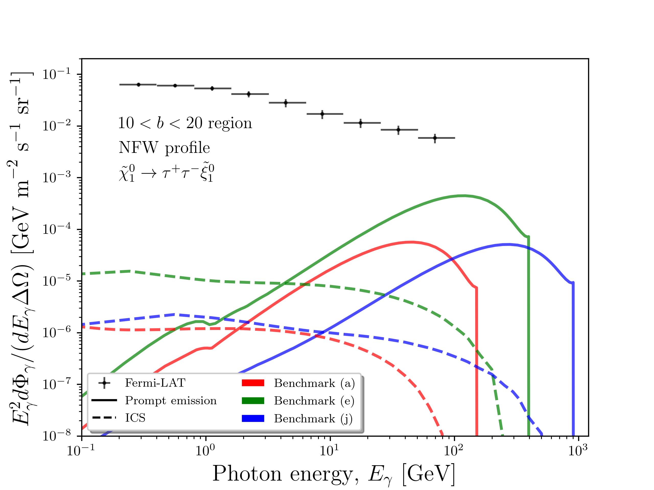
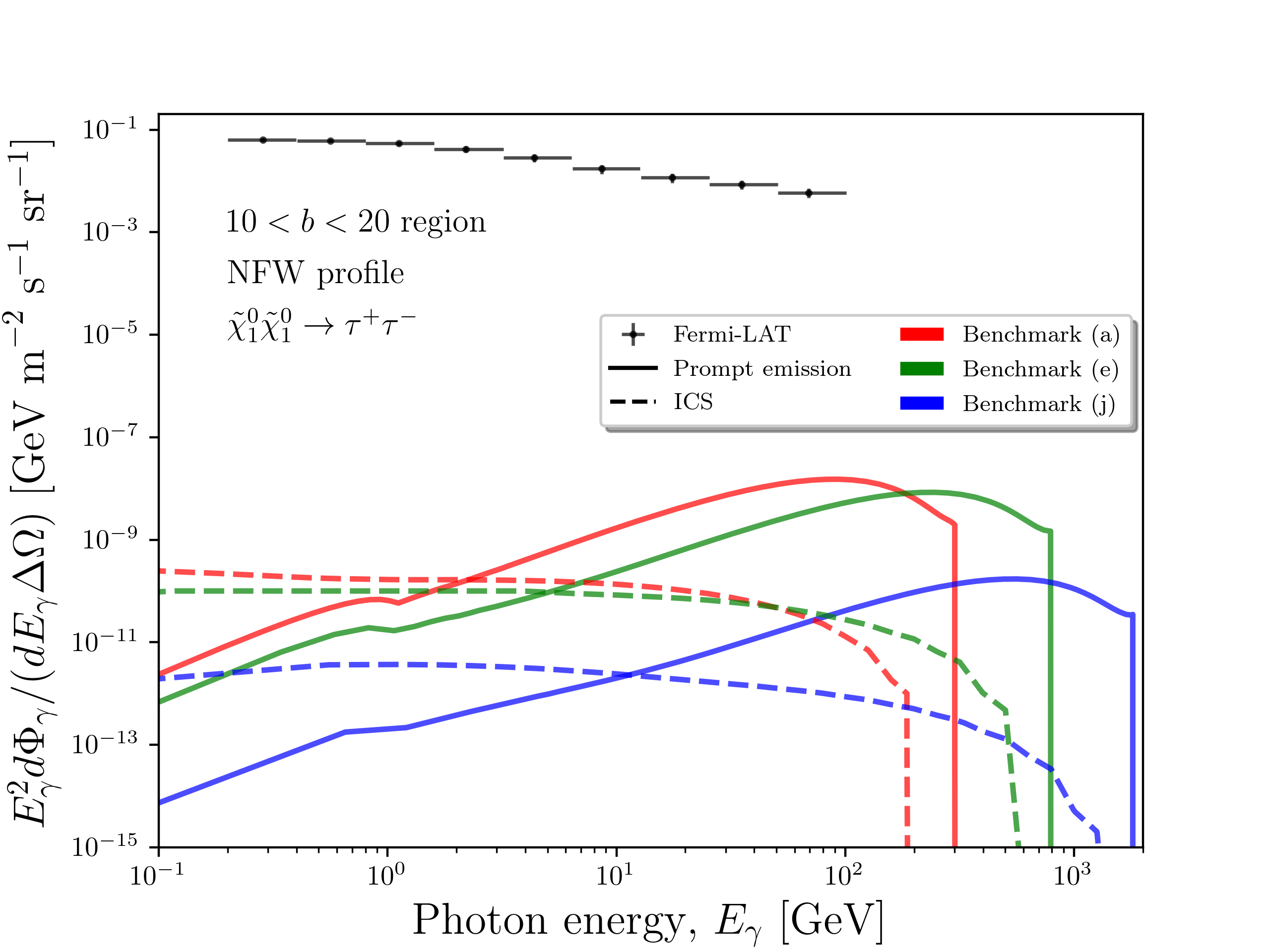
Figure 2: The gamma ray flux from the decay (left panel) and annihilation (right panel) of $\tilde{\chi}_{1}^{0}$ for three benchmarks of Table 1 due to prompt emission and ICS. Also shown are the Fermi-LAT data points.

It is seen in Fig. 2 that ICS dominates over prompt photons for small energies while prompt photons have higher intensities for higher energies which is consistent with a photon spectrum obtained from pion decays. Also plotted are the Fermi-LAT data points in the same region of observation. For both cases of decay and annihilation, the sum of prompt and secondary photons’ flux is below the observed gamma ray flux.

Since taus can decay hadronically, it is important to make sure that the antiproton flux from decay and annihilation of DM does not exceed the antiproton background. This background fits well the estimates from known astrophysical processes and allows very little room for additional hadronic decays or annihilation of DM. Despite the reported excesses which were discussed in the introduction, uncertainties in the DM density profiles, the propagation parameters used in solving the antiproton transport equation and solar modulation can wash away the excess at low energy while the higher energy excess can be argued away due to astrophysical processes. The antiproton flux for three benchmarks of Table 1 is calculated using Eqs. (B.10) and (B.11) and plotted against the antiproton energy in the left panel of Fig. 3. The recent AMS-02 data [7] is shown along the estimated background fit.

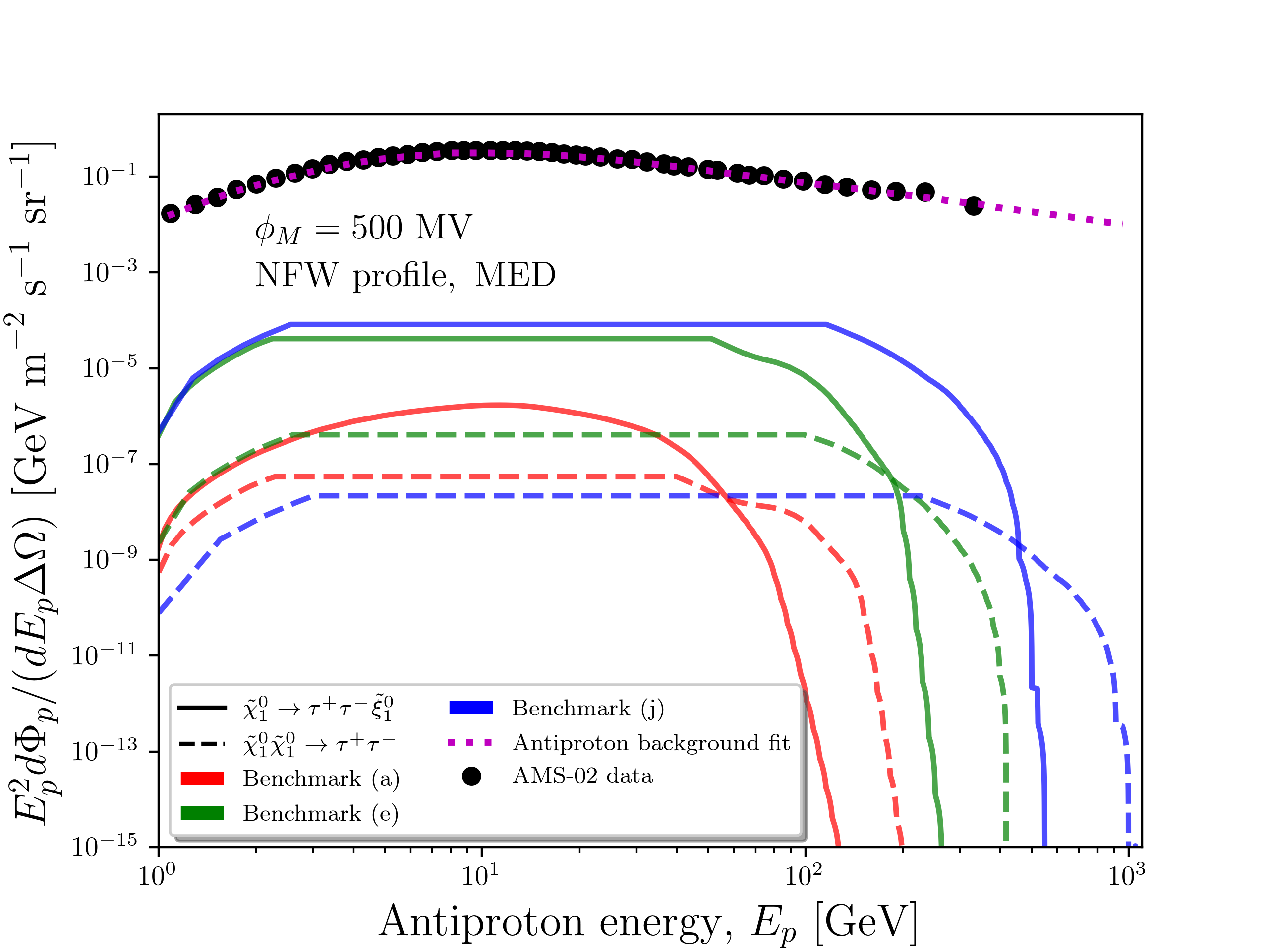
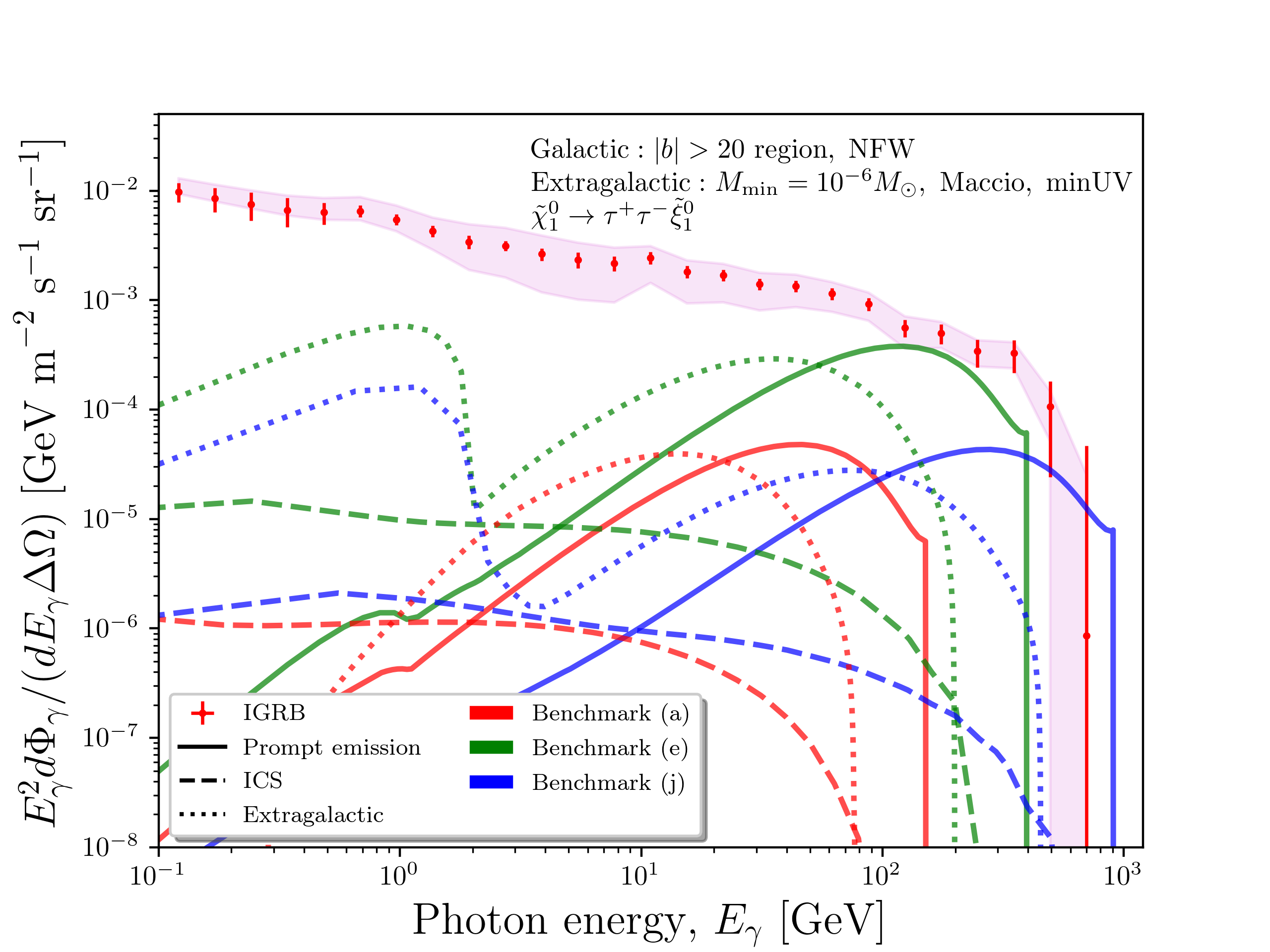
Figure 3: Left panel: Contributions from the annihilation and decay of the MSSM neutralino $\tilde{\chi}^{0}_{1}$ to the antiproton flux for three of the benchmarks of Table 1. The antiproton background and AMS data are also shown. Right panel: the gamma ray flux from the IGRB (for decay only) showing contributions from prompt photons, ICS and extragalatic photons. Fermi-LAT data points are in red with error bars and the uncertainty band from foreground modeling.

The antiproton fluxes coming from the decay and annihilation of DM for the benchmarks of Table 1 lie well below the observed background. Another possible antimatter channel is that of positrons. Since the leptonic decays of taus are smaller than the hadronic ones, one can safely assume that our benchmarks do not contribute to the observed positron excess and so is not constraining for the model. In the right panel of Fig. 3 we show contributions from DM decay to the IGRB for three benchmarks of Table 1. Photon emission from prompt decay (solid line) and ICS (dashed line) as well as the extragalactic component (dotted line) lie below the diffuse IGRB measured by Fermi-LAT [55] and shown as red points with error bars due to systematic and statistical uncertainties. The magenta band corresponds to uncertainties on IGRB from foreground modeling. The case of annihilation is not shown since it is much smaller than the decay case and therefore can be neglected.

There are several experiments planned or are underway on indirect detection of decaying DM signatures. One of these is the Square Kilometer Array (SKA) [9] which can reach high frequencies and would be a suitable probe of the high DM masses. SKA is expected to have improved efficiency in separating foregrounds thanks to its intercontinental baseline length and large effective area. In regards to the DM decay lifetime, SKA can reach 2 to 3 orders of magnitude in sensitivity higher than Fermi-LAT [10] for DM masses up to 100 TeV. Another telescope array known as Cherenkov Telescope Array (CTA) [11] is being built with more than 100 telescopes in the Northern and Southern hemispheres. CTA will scan the skies looking for high energy gamma rays and will be 10 times more sensitive than H.E.S.S. [12, 13], MAGIC [14, 15] and VERITAS [16, 17].

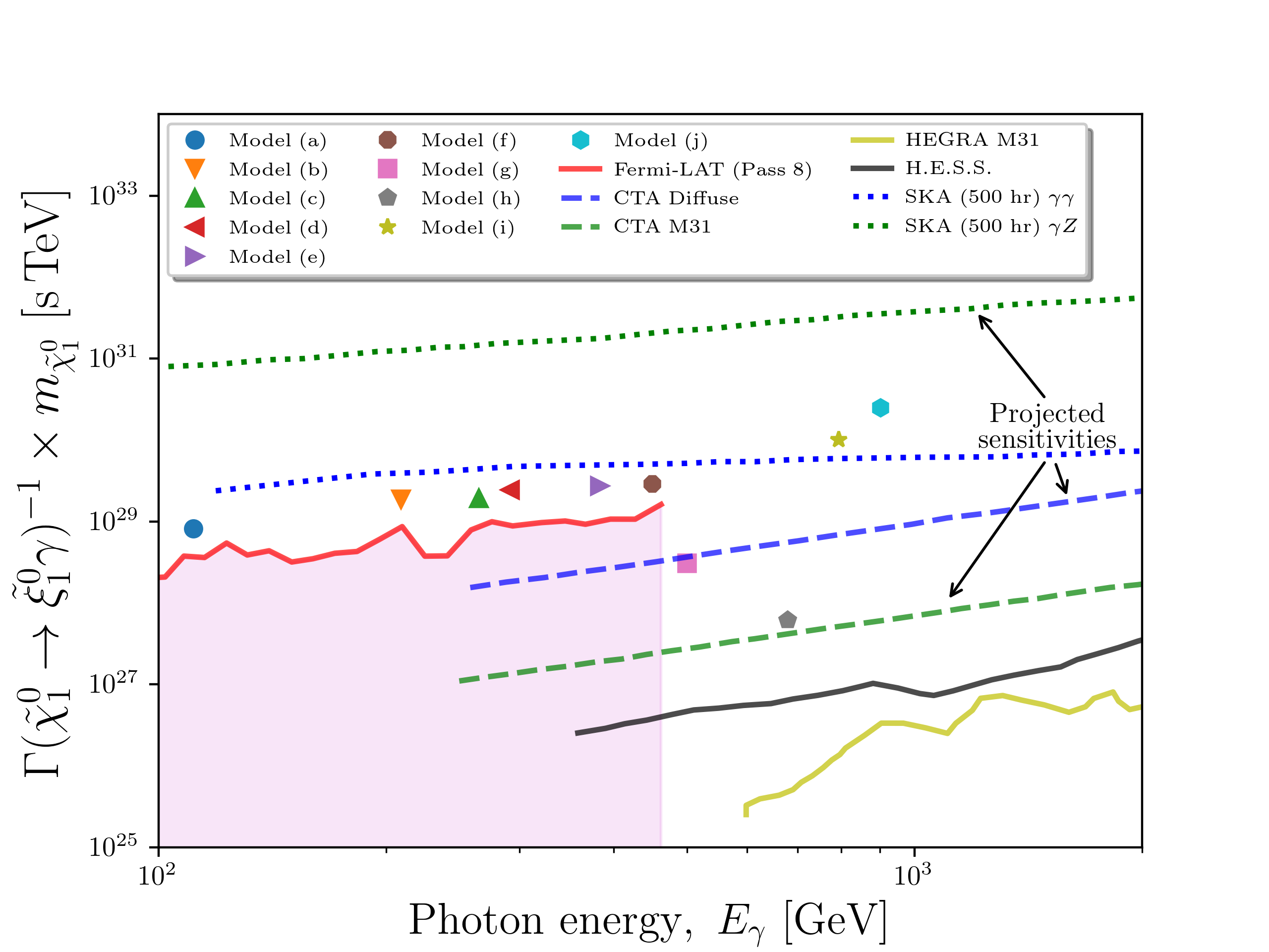
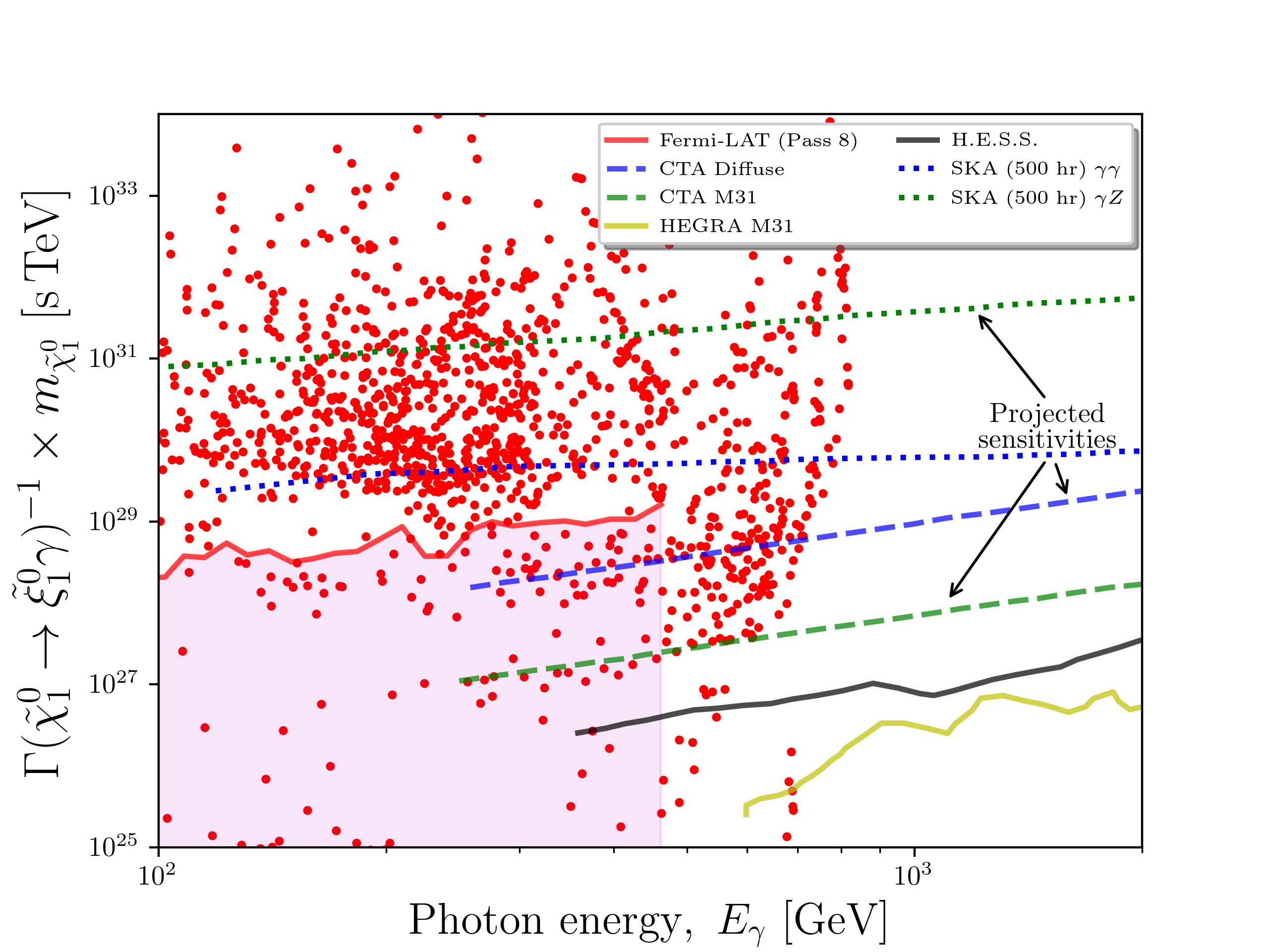
Figure 4: Left panel: A plot of $m_{\tilde{\chi}^{0}_{1}}/\Gamma(\tilde{\chi}^{0}_{1}\rightarrow\tilde{\xi}^{0}_{1}\gamma)$, in TeV s, versus the photon energy in GeV for a set of ten benchmarks consistent with all collider and astrophysical constraints. The model points are accessible in future improved experiments. Right panel: A scatter plot in the same variables shows that the parameter space in which a decaying neutralino consistent with all the current constraints can reside is quite large and a significant part of the parameter space will be accessible to more sensitive future experiments such as SKA and CTA [18, 19]. The ranges of the scanned parameters are: $800~{}\text{GeV}<m_{0}<5~{}\text{TeV}$, $-5<A_{0}/m_{0}<5$, $700~{}\text{GeV}<m_{1}<5.5~{}\text{TeV}$, $400~{}\text{GeV}<m_{2}<4~{}\text{TeV}$, $2~{}\text{TeV}<m_{3}<6.5~{}\text{TeV}$, $1<\tan\beta<50$, $500~{}\text{GeV}<M_{1}<5~{}\text{TeV}$ and $m_{X_{2}}=6$ TeV. The current and future limits from dark matter indirect detection experiments are shown in both panels.

Since the benchmarks of Table 1 satisfy all the indirect detection constraints, we can now use them to investigate the possibility of observing a sharp monochromatic spectral line in the decay $\tilde{\chi}^{0}_{1}\to\tilde{\xi}^{0}_{1}\gamma$. In Fig. 4, we exhibit $m_{\tilde{\chi}^{0}_{1}}/\Gamma(\tilde{\chi}^{0}_{1}\rightarrow\tilde{\xi}^{0}_{1}\gamma)$ plotted against the photon energy for the benchmarks of Table 1 (left panel). We also exhibit the current limits from Fermi-LAT [53, 20], HEGRA [67] and H.E.S.S. [12, 13] as well as the projections from the future CTA and SKA experiments. The limits from SKA are derived from the $\gamma\gamma$ and $\gamma Z$ channels assuming 500 hours of operation. One can notice that the limit from $\gamma Z$ is more stringent since $Z$ fragments into visible SM particles. Here one finds that none of the model points of Table 1 are yet excluded by experiment. Thus benchmarks (a)$-$(f) lie just above the current Fermi-LAT limit and can be probed with higher sensitivities while the rest of the benchmarks are well within the range of detectability of CTA and SKA. It should be noted that there are many limits set on decaying DM in the literature [21, 22, 23, 24, 25, 26, 27, 28, 29]. These analyses give limits on the DM lifetime to be $\mathcal{O}(10^{27-28})$ s with the exception of light DM (in the MeV$-$GeV range) where the constraints are less stringent. In Ref. [30], data from HEAO-1 [31], INTEGRAL [32], COMPTEL [33] and EGRET [34] were used to set limits on decaying light DM particles. Furthermore, using a microwave background analysis, one sets a limit on the lifetime of DM decaying to 30 MeV electrons and positrons [35] to be greater than $2.6\times 10^{25}$ s, at 95% CL. Scanning the parameter space of the model, one finds many more points that can be probed by future experiments in a wide range of photon energy. Those points are shown in the right panel of Fig. 4. We note that the sharp cutoff of model points in the scatter plot is due to the limits placed on the parameter space of input used in generating the scatter plot. Just as for the benchmarks of Table 1, the model points in the scatter plot have enhanced leptonic (mostly tau) three body decays with an estimated flux below the limits shown in Fig. 2 and Fig. 3. The discovery of a monochromatic spectral line feature would be a strong evidence for a decaying dark matter since standard astrophysical processes do not produce such an effect.

5 Conclusions

The search for dark matter has resulted in both direct and indirect detection experiments. Direct detection involves either producing the DM particles directly using collider experiments such as the LHC or using large volume underground experiments such as Xenon1T and the upcoming XenonnT to measure electronic or nuclear recoil effects as DM particles scatter off xenon atoms. Most recently, Xenon1T [68] detected some excess in electronic recoil events in the few keV region with hidden sector DM as a possible explanation (see, e.g., [69] and the references therein). However, a radioactive tritium background cannot be ruled out as a possible reason for such an excess. Indirect detection experiments have been reporting several signals for possible DM particles through their annihilation or decay products such as the positron excess by the PAMELA [1] and AMS-02 [4, 5, 6] experiments. In contrast to charged particles which cannot be easily traced back to their origin due to energy losses and diffusion as those particles travel through the universe, gamma ray signals do not suffer from those uncertainties and can be a powerful tool in searching for DM.

In this work we have investigated the possibility of detecting a monochromatic gamma ray line resulting from the radiative decay of a long-lived MSSM/SUGRA neutralino $\tilde{\chi}^{0}_{1}$ into the hidden sector fermion $\tilde{\xi}^{0}_{1}$ in the process $\tilde{\chi}^{0}_{1}\to\tilde{\xi}^{0}_{1}\gamma$. With mixing between the visible sector and the hidden sector neutralino $\tilde{\xi}_{1}^{0}$ chosen to be ultraweak, the lifetime for the decay of the neutralino is much larger than the lifetime of the universe. Thus it was shown that the MSSM/SUGRA neutralino of the visible sector, although unstable, can generate the full dark matter relic density of the universe. At the same time, production of the hidden sector neutralino is suppressed in the early universe because of its ultraweak interactions with the SM particles. Further, the amount of hidden sector neutralino $\tilde{\xi}^{0}_{1}$ produced via the decay of the visible sector neutralino is negligible because the decay lifetime of the visible sector neutralino is significantly larger than the lifetime of the universe. Thus the MSSM/SUGRA neutralino of the visible sector is the dominant component of dark matter in the universe at current times with the hidden sector neutralino $\tilde{\xi}_{1}^{0}$ being a subdominant component.

To investigate in a quantitative fashion the possibility of detection of the monochromatic gamma ray signal in the model, we generated a number of benchmarks given in Table 1. To ensure the viability of the benchmarks we investigated the diffuse gamma ray emission which can arise in this model from three body decays such as $\tilde{\chi}^{0}_{1}\to\tilde{\xi}^{0}_{1}f\bar{f}$, where the final state is dominated by $\tau^{+}\tau^{-}$. Similarly, the DM annihilation is dominated by the channel $\tilde{\chi}^{0}_{1}\tilde{\chi}^{0}_{1}\to\tau^{+}\tau^{-}$. These decays produce diffuse photons and we showed that the produced photon fluxes do not exceed the current limit from Fermi-LAT allowing for a monochromatic photon line to be observed in current and future experiments with greater sensitivity such as SKA and CTA. We also showed that the antiproton flux arising from these decays and annihilation for the benchmarks makes a very suppressed contribution to the antiproton background from astrophysical sources. It is remarkable that despite the fact that line emissions are loop suppressed compared to diffuse emissions from three-body decays, the former can still produce a signal that may be detectable in future experiments.

Finally, we point to the new elements of the analysis and compare our work to the existing literature. The model discussed in section 2 is an extended $\text{MSSM/SUGRA}\times U(1)_{X_{1}}\times U(1)_{X_{2}}$ model with 8 neutralinos involving kinetic mixing of three $U(1)^{\prime}s$, i.e., $U(1)_{Y}\times U(1)_{X_{1}}\times U(1)_{X_{2}}$, where the visible sector communicates with the hidden sector $X_{2}$ only via the sector $X_{1}$ making the coupling of the visible sector with $X_{2}$ doubly suppressed. This mechanism is helpful in allowing the visible sector neutralino to decay into the lighter neutralino in $X_{2}$ with lifetime larger that the age of the universe with couplings of two $U(1)$’s of size $\mathcal{O}(10^{-12})$. This is to be contrasted with the case of just one $U(1)_{X}$ which would require a mixing of size $\mathcal{O}(10^{-24})$. While the ultraweak mixings of size $\mathcal{O}(10^{-12})-\mathcal{O}(10^{-24})$ can be manufactured in string compactifications, we believe that mixings of size $\mathcal{O}(10^{-12})$ offer less fine tuned solutions than those of size $\mathcal{O}(10^{-24})$. However, this is to a degree subjective. In any case, the proposed mechanism of section 2 is new and offers another solution to achieving ultraweak mixings. Regarding sections A and 3, here the first complete analysis of $W$-charginos, charged Higgs-charginos, and fermion-sfermions exchange contributions in the loops is given. The parameter space of the model is constrained by the astrophysical and laboratory constraints which include the relic density, the gamma ray flux and antiproton flux. The monochromatic signal is analysed in detail.

We now compare our analysis to previous works. While decaying dark matter has been discussed by various authors there is currently no focused work on the decaying neutralino in the framework we discuss. Thus, while the work of [70] discusses decaying neutralino as dark matter, the analysis is within the framework of $R$-parity violation and has no overlap with our work. In our analysis, $R$-parity is strictly conserved and the decay of the neutralino arises at the loop level. The work of Ref. [51] does consider mSUGRA model points but is restricted to leptonic three-body decays to explain the positron excess and does not discuss the radiative two body decay of the neutralino. Ref. [18] discusses radiative decay but the analysis is in a non-supersymmetric framework with a brief discussion of the SUSY case. Further, the model assumes the dark matter to be leptophilic to avoid hadronic decays of DM. In our analysis a natural suppression of hadronic channels occurs due to a light stau as discussed in the text. Moreover, our analysis is consistent with the observed Higgs boson mass and the relic density constraint which are overlooked in some of the previous analyses. Finally, the analyses of Figs. 3 and 4 takes account of the most recent experimental limits from Fermi-LAT and CTA and discusses the prospects of the new SKA experiment.

Acknowledgments: The research of AA and MK was supported by the BMBF under contract 05H18PMCC1, while the research of PN was supported in part by the NSF Grant PHY-1913328.

Appendices

Appendix A Interactions that enter in the analysis of the neutralino radiative decay

The radiative neutralino decay $\tilde{\chi}_{1}^{0}\to\tilde{\xi}_{1}^{0}\gamma$ is a loop suppressed process and the loop diagrams contributing to it are given in Fig. 1. The loop diagrams involve the following interactions: $WW\gamma$, chargino-chargino-$\gamma$, neutralino-chargino-$W$, neutralino-fermion-sfermion and neutralino-chargino-charged Higgs. We discuss them below.

The $WW\gamma$ coupling is obtained from the triboson Lagrangian

$$\mathcal{L}_{V} =ie\cot{\theta_{W}}\left[\left(\partial^{\mu}W^{\nu}-\partial^{\nu}W^{\mu}\right)W^{\dagger}_{\mu}Z_{\nu}-\left(\partial^{\mu}W^{\nu\dagger}-\partial^{\nu}W^{\mu\dagger}\right)W_{\mu}Z_{\nu}+W_{\mu}W^{\dagger}_{\nu}\left(\partial^{\mu}Z^{\nu}-\partial^{\nu}Z^{\mu}\right)\right]$$

$$+ie\left[\left(\partial^{\mu}W^{\nu}-\partial^{\nu}W^{\mu}\right)W^{\dagger}_{\mu}A_{\nu}-\left(\partial^{\mu}W^{\nu\dagger}-\partial^{\nu}W^{\mu\dagger}\right)W_{\mu}A_{\nu}+W_{\mu}W^{\dagger}_{\nu}\left(\partial^{\mu}A^{\nu}-\partial^{\nu}A^{\mu}\right)\right].$$ (A.1)

The chargino-chargino-$\gamma$ coupling is given by

$$\mathcal{L}_{\tilde{\chi}\gamma}=-eA_{\mu}\bar{\chi}^{C}\gamma^{\mu}\chi^{C}\,,$$ (A.2)

while the neutralino-chargino-$W$ coupling is given by

$$\mathcal{L}_{\tilde{\chi}^{0}\tilde{\chi}W}=g_{2}W_{\mu}^{-}\bar{\chi_{i}}^{0}\gamma^{\mu}\left(O^{L}_{ij}P_{L}+O^{R}_{ij}P_{R}\right)\chi_{j}^{C}+\text{h.c.},$$ (A.3)

with

$$O^{L}_{ij} =-\frac{1}{\sqrt{2}}X_{i4}V^{*}_{j2}+X_{i2}V^{*}_{j1},$$

$$O^{R}_{ij} =\frac{1}{\sqrt{2}}X^{*}_{i3}U_{j2}+X^{*}_{i2}U_{j1},$$ (A.4)

where $X$ diagonalizes the neutralino mass matrix $M_{N}$ of Eq. (2.8) so that

$$X^{*}M_{N}X^{-1}=\text{ diag}(m_{\tilde{\chi}_{1}^{0}},m_{\tilde{\chi}_{2}^{0}},m_{\tilde{\chi}_{3}^{0}},m_{\tilde{\chi}_{4}^{0}},m_{\tilde{\chi}_{5}^{0}},m_{\tilde{\chi}_{6}^{0}},m_{\tilde{\chi}_{7}^{0}},m_{\tilde{\chi}_{8}^{0}}),$$ (A.5)

and $\tilde{\xi}^{0}_{4}\equiv\tilde{\chi}_{5}^{0},~{}\tilde{\xi}^{0}_{3}\equiv\tilde{\chi}_{6}^{0},~{}\tilde{\xi}^{0}_{2}\equiv\tilde{\chi}_{7}^{0},~{}\tilde{\xi}^{0}_{1}\equiv\tilde{\chi}_{8}^{0}$. The Majorana phases are absorbed into $X$ so that the masses are non-negative. The $U$ and $V$ are the matrices that diagonalize the chargino mass matrix so that

$$U^{*}M_{C}V^{-1}=\text{ diag}(m_{\tilde{\chi}_{1}^{\pm}},m_{\tilde{\chi}_{2}^{\pm}}),$$ (A.6)

where $M_{C}$ is the chargino mass matrix.

A.1 The effective Lagrangian for $\bar{q}\tilde{q}_{i}\tilde{\chi}_{j}^{0}$ interaction

The quark-squark-neutralino, $\bar{q}\tilde{q}_{i}\chi_{j}^{0}$, interaction at the tree level is given by

$$\mathcal{L}_{q\tilde{q}\tilde{\chi}^{0}}=g\bar{d}(K^{d}_{ij}P_{R}+M^{d}_{ij}P_{L})\tilde{\chi}_{j}^{0}\tilde{d}_{i}+g\bar{u}(K^{u}_{ij}P_{R}+M^{u}_{ij}P_{L})\tilde{\chi}_{j}^{0}\tilde{u}_{i}+\text{h.c.}$$ (A.7)

Here $i=1,2$ stand for the two squark states (first generation sup and sdown), $j=1\cdots 8$ stand for the 8 neutralino states and where the couplings in Eq. (A.7) are given by

$$K^{d}_{ij} =-\sqrt{2}(\beta_{dj}D_{d1i}+\alpha_{dj}^{*}D_{d2i}),$$ (A.8)

$$K^{u}_{ij} =-\sqrt{2}(\beta_{uj}D_{u1i}+\alpha_{uj}^{*}D_{u2i}),$$

$$M^{d}_{ij} =-\sqrt{2}(\alpha_{dj}D_{d1i}-\gamma_{dj}D_{d2i}),$$

$$M^{u}_{ij} =-\sqrt{2}(\alpha_{uj}D_{u1i}-\gamma_{uj}D_{u2i}).$$

The quantity $D_{q}$ (with $q=u,d$) in Eq. (A.8) is the matrix that diagonalizes the squark mass square matrix, $M_{\tilde{q}}^{2}$, i.e.,

$$D_{q}^{\dagger}M_{\tilde{q}}^{2}D_{q}={\rm diag}(m_{\tilde{q}1}^{2},m_{\tilde{q}2}^{2}),$$ (A.9)

where $M_{\tilde{q}}^{2}$ is given by

$$\left(\begin{matrix}M_{\tilde{Q}}^{2}+m{{}_{q}}^{2}+M_{Z}^{2}(\frac{1}{2}-Q_{q}\sin^{2}\theta_{W})\cos 2\beta&m_{q}(A_{q}-\mu R_{q})\cr m_{q}(A_{q}-\mu R_{q})&M_{\tilde{U}}^{2}+m{{}_{q}}^{2}+M_{Z}^{2}Q_{q}\sin^{2}\theta_{W}\cos 2\beta\end{matrix}\right).$$ (A.10)

Here $Q_{q}=2/3(-1/3)$ and $R_{q}=\cot\beta(\tan\beta)$ for $q=u(d)$, and $m_{q}$ is the quark mass. The various other quantities appearing in Eq. (A.8) are defined as follows [43]

$$\alpha_{d(u)k} =\frac{gm_{d(u)}X_{3(4)k}}{2m_{W}\cos\beta(\sin\beta)},~{}~{}~{}\beta_{d(u)k}=eQ_{d(u)}X_{1k}^{{}^{\prime}*}+\frac{g}{\cos\theta_{W}}X_{2k}^{{}^{\prime}*}(T_{3d(u)}-Q_{d(u)}\sin^{2}\theta_{W}),$$ (A.11)

$$\gamma_{d(u)k} =eQ_{d(u)}X_{1k}^{\prime}-\frac{gQ_{d(u)}\sin^{2}\theta_{W}}{\cos\theta_{W}}X_{2k}^{\prime},$$

where $T_{3d}=-\frac{1}{2}$, $T_{3u}=\frac{1}{2}$, $Q_{d}=-\frac{1}{3}$, $Q_{u}=\frac{2}{3}$ and the $X^{\prime}$’s are given in terms of $X$, the matrix that diagonalizes the neutralino mass matrix, as

$$X^{\prime}_{1k} =X_{1k}\cos\theta_{W}+X_{2k}\sin\theta_{W},$$ (A.12)

$$X^{\prime}_{2k} =-X_{1k}\sin\theta_{W}+X_{2k}\cos\theta_{W}.$$

The same analysis can be easily generalized to include the second and third generation quarks and squarks. To extract the interactions of the MSSM neutralino $\tilde{\chi}^{0}_{1}$ from Eq. (A.7) we set $j=1$ while setting $j=8$ allows one to obtain the interactions of the LSP, $\tilde{\xi}^{0}_{1}$.

A.2 The effective Lagrangian for $\bar{\ell}\tilde{\chi}_{i}^{0}\tilde{\ell}_{j}$ interaction

To determine the elements of this interaction, we start by writing the slepton mass square matrix. It is given by

$$M_{\tilde{{\ell}}}^{2}=\left(\begin{matrix}M_{\tilde{L}}^{2}+m{{}_{{\ell}}}^{2}-M_{Z}^{2}(\frac{1}{2}-\sin^{2}\theta_{W})\cos 2\beta&m_{{\ell}}(A_{{\ell}}-\mu\tan\beta)\cr m_{{\ell}}(A_{{\ell}}-{\mu}\tan\beta)&M_{\tilde{R}}^{2}+m{{}_{\ell}}^{2}-M_{Z}^{2}\sin^{2}\theta_{W}\cos 2\beta\end{matrix}\right),$$ (A.13)

which is a hermitian matrix and can be diagonalized by the unitary transformation

$$D_{{\ell}}^{\dagger}M_{\tilde{{\ell}}}^{2}D_{{\ell}}={\rm diag}(m_{\tilde{{\ell}}1}^{2},m_{\tilde{{\ell}}2}^{2}).$$ (A.14)

The neutralino-lepton-slepton interaction in the mass diagonal basis is defined by

$$-\mathcal{L}_{\ell\tilde{\ell}\tilde{\chi}^{0}}=\bar{\ell}(F_{ij}P_{L}+Z_{ij}P_{R})\tilde{\chi}^{0}_{i}\tilde{\ell}_{j}+\text{h.c.},$$ (A.15)

where the couplings $F_{ij}$ and $Z_{ij}$ are given by

$$F_{ij} =\sqrt{2}(\alpha_{\ell i}D_{\ell 1j}-\gamma_{\ell i}D_{\ell 2j}),$$ (A.16)

$$Z_{ij} =\sqrt{2}(\beta_{\ell i}D_{\ell 1j}-\delta_{\ell i}D_{\ell 2j}),$$

and the quantities $\alpha$, $\beta$, $\gamma$ and $\delta$ are

$$\alpha_{{\ell}i} =\frac{gm_{{\ell}}X_{3i}}{2m_{W}\cos{\beta}},~{}~{}~{}\beta_{{\ell}i}=eQ_{{\ell}}X_{1i}^{{}^{\prime}*}+\frac{g}{\cos{\theta_{W}}}X_{2i}^{{}^{\prime}*}(T_{3{\ell}}-Q_{{\ell}}\sin^{2}{\theta_{W}}),$$ (A.17)

$$\gamma_{{\ell}i} =eQ_{{\ell}}X_{1i}^{{}^{\prime}}-\frac{gQ_{{\ell}}\sin^{2}{\theta_{W}}}{\cos{\theta_{W}}}X_{2i}^{{}^{\prime}},~{}~{}~{}\delta_{{\ell}i}=-\frac{gm_{{\ell}}X_{3i}^{*}}{2m_{W}\cos{\beta}}.$$

Again, the $\tilde{\chi}_{1}^{0}\ell\tilde{\ell}$ interaction can be gotten by setting $i=1$ and $\tilde{\xi}_{1}^{0}\ell\tilde{\ell}$ is obtained for $i=8$.

A.3 The effective Lagrangian for $H^{-}\tilde{\chi}^{0}_{i}\tilde{\chi}^{+}_{j}$ interaction

The effective Lagrangian that describes the charged Higgs-chargino-neutralino vertex is given by

$${\cal{L}}_{H\tilde{\chi}^{0}\tilde{\chi}^{+}}=H^{-}\bar{\tilde{\chi}}^{0}_{i}(\alpha^{S}_{ij}+\gamma_{5}\alpha^{P}_{ij})\tilde{\chi}^{+}_{j}+\text{h.c.},$$ (A.18)

where $i=1\cdots 8$, $j=1,2$ and

$$\alpha^{S}_{ij} =\frac{1}{2}\xi^{\prime}_{ij}\sin{\beta}+\frac{1}{2}\xi_{ij}\cos{\beta},$$ (A.19)

$$\alpha^{P}_{ij} =\frac{1}{2}\xi^{\prime}_{ij}\sin{\beta}-\frac{1}{2}\xi_{ij}\cos{\beta}.$$

In the above, $\xi_{ij}$ and $\xi_{ij}^{\prime}$ are given by

$$\xi_{ij} =-gX_{4i}V_{j1}^{*}-\frac{g}{\sqrt{2}}X_{2i}V_{j2}^{*}-\frac{g}{\sqrt{2}}\tan\theta_{W}X_{1i}V_{j2}^{*},$$ (A.20)

$$\xi_{ij}^{\prime} =-gX_{3i}^{*}U_{j1}+\frac{g}{\sqrt{2}}X_{2i}^{*}U_{j2}+\frac{g}{\sqrt{2}}\tan\theta_{W}X_{1i}^{*}U_{j2}.$$

To obtain the interactions of $\tilde{\chi}^{0}_{1}$ we set $i=1$ and for $\tilde{\xi}^{0}_{1}$ we set $i=8$.

Appendix B The flux from relevant astrophysical processes

The main source of gamma ray photons reaching terrestrial detectors arises from the galactic center (GC). Those photons can be prompt, i.e. the result of internal bremsstrahlung, or come from the decay of SM hadrons or decay/annihilation of DM particles. Secondary sources of photons are due to inverse Compton scattering (ICS), bremsstrahlung and synchrotron emission. In this work, prompt emissions and ICS dominate for the energy range and observational region of interest. The photon flux from the GC depends on the DM density profile which we consider to be of the Navarro, Frenk and White (NFW) form [44]. In this Appendix we give details of the calculations of the gamma ray flux from prompt photons, ICS and IGRB as well as the antiproton flux.

B.1 Prompt $\gamma$ ray photons

SM final states (leptons, quarks, $W^{\pm}$, $Z$) resulting from the decay or annihilation of DM particles in the GC will give rise to a continuum and diffuse photon spectrum. Photons are produced either by final state radiation off charged particles or by the decay of hadrons, such as pions. The spectrum has a kinematic endpoint at half the DM mass for decay processes and at the dark matter mass for annihilation.
The differential photon flux for an observation region $\Delta\Omega$ is given by

$$\frac{d\Phi}{dE\Delta\Omega}(E_{\gamma})=\frac{r_{\odot}}{4\pi}\frac{\rho_{\odot}}{m_{\tilde{\chi}^{0}_{1}}}\bar{J}\sum_{i}\frac{1}{\tau_{i}}\frac{dN_{i}}{dE_{\gamma}},$$ (B.1)

where $dN_{i}/dE_{\gamma}$ is the photon spectrum produced from the decay into some final state $i$ and is determined using PYTHIA [45], $\tau_{i}$ is the DM lifetime, $\bar{J}$ is the average $J$ factor for prompt photons given by

$$\bar{J}=\frac{4}{\Delta\Omega}\iint db\,d\ell\cos b\,J[\theta(b,\ell)],$$ (B.2)

in the $b\times\ell$ region with $(b,\ell)$ being the galactic coordinates (latitude $b$ and longitude $\ell$) and

$$\Delta\Omega=4\iint db\,d\ell\cos b.$$ (B.3)

The $J$ factor, $J(\theta)$ is calculated with PPPC4DMID [47, 48] where $\cos\theta=\cos b\cos\ell$ near the galactic plane. Note that $\theta$ is the aperture angle between the direction of the line of sight and the axis connecting the Earth to the GC. $r_{\odot}$ is the location of the Sun in the galactic plane which we take to be 8.5 kpc and $\rho_{\odot}=0.4$ GeV/cm³ is the DM mass density at $r_{\odot}$.

One can write a similar expression for the photon flux for annihilation processes

$$\frac{d\Phi}{dE\Delta\Omega}(E_{\gamma})=\frac{r_{\odot}}{4\pi}\frac{1}{2}\left(\frac{\rho_{\odot}}{m_{\tilde{\chi}^{0}_{1}}}\right)^{2}\bar{J}\sum_{i}\langle\sigma v\rangle_{i}\frac{dN_{i}}{dE_{\gamma}},$$ (B.4)

where $\langle\sigma v\rangle_{i}$ is the DM thermally averaged cross-section into some final states $i$. This diffuse and broad spectrum of photon emission from DM particles is hard to disentangle from astrophysical processes which constitute an overwhelming background.

The direct decay/annihilation of DM particles to photons will produce a sharp spectral line which can be easily detected over the otherwise smooth background from astrophysical emissions. Such a spectral line would be centered at

$$E_{\gamma}=\frac{m_{\tilde{\chi}^{0}_{1}}}{2}\left(1-\frac{m^{2}_{\tilde{\xi}^{0}_{1}}}{m^{2}_{\tilde{\chi}^{0}_{1}}}\right),$$ (B.5)

for the decay $\tilde{\chi}^{0}_{1}\to\tilde{\xi}^{0}_{1}\gamma$ and at $E_{\gamma}=m_{\tilde{\chi}^{0}_{1}}$ for annihilation $\tilde{\chi}^{0}_{1}\tilde{\chi}^{0}_{1}\to\gamma\gamma$. In this case, the photon spectrum becomes $dN/dE_{\gamma}=\delta(E-E_{\gamma})$ for decay and $2\delta(E-E_{\gamma})$ for annihilation.

B.2 Inverse Compton scattering

Photon flux signals generated in the GC are generally the most intense but are plagued with high levels of astrophysical background processes. At higher latitudes the signal becomes weaker and so does the contamination from the background. Energetic SM final states such as electrons arising from the decay or annihilation of DM particles can scatter off the interstellar light and the cosmic microwave background (CMB) sending those soft photons into the gamma ray energy range. Such a process is known as ICS. The photon signal from ICS comes from every direction in the diffusion volume of the galactic halo including high latitudes where astrophysical processes are subdominant and thus suffers from less uncertainties compared to the signal from the GC.

Products of DM decay or annihilation can be grouped into primary, $p$, and secondary, $s$. Primary particles are the result of the immediate decay/annihilation while secondary particles are stable SM particles resulting from the cascade decays of the primary particles. For ICS, electrons and positrons are the relevant secondary particles responsible for this scattering process. The differential ICS photon flux in the case of DM decay is given by

$$\frac{d\Phi_{\rm ICS}}{dE_{\gamma}\Delta\Omega}=\frac{r_{\odot}}{4\pi}\frac{\rho_{\odot}}{m_{\tilde{\chi}^{0}_{1}}}\frac{1}{E^{2}_{\gamma}}\int_{m_{s}}^{m_{\tilde{\chi}^{0}_{1}}/2}dE_{s}\sum_{i}\frac{1}{\tau_{i}}\frac{dN^{i}_{s}}{dE}(E_{s})F_{\rm ICS}(E_{\gamma},E_{s},b,\ell),$$ (B.6)

where $E_{s}$ and $m_{s}$ are the injection energy and mass of the secondary particle (in this case $e^{\pm}$) and $F_{\rm ICS}$ is a Halo function determined using the NFW profile and a set of propagation parameters [49]. For the DM annihilation case, the differential flux takes the form

$$\frac{d\Phi_{\rm ICS}}{dE_{\gamma}\Delta\Omega}=\frac{r_{\odot}}{4\pi}\left(\frac{\rho_{\odot}}{m_{\tilde{\chi}^{0}_{1}}}\right)^{2}\frac{1}{2E^{2}_{\gamma}}\int_{m_{s}}^{m_{\tilde{\chi}^{0}_{1}}}dE_{s}\sum_{i}\langle\sigma v\rangle_{i}\frac{dN^{i}_{s}}{dE}(E_{s})F_{\rm ICS}(E_{\gamma},E_{s},b,\ell).$$ (B.7)

B.3 Antiproton flux

The production and propagation of cosmic rays in the galaxy is a complicated process since it requires a modeling of diffusion, energy loss and annihilation effects as the charged particles navigate through the magnetic field of the galaxy. This process is generally described by a transport equation which arises from a stationary two-zone diffusion model with cylindrical boundary conditions [50, 51]. For the case of antiprotons of mass $m_{p}$ resulting from DM decay, the solution to the transport equation at the position of the solar system is given by

$$f(E)=\frac{1}{\tau m_{\tilde{\chi}^{0}_{1}}}\int_{0}^{m_{\tilde{\chi}^{0}_{1}}-m_{p}}dE^{\prime}\,G(E,E^{\prime})\frac{dN(E^{\prime})}{dE^{\prime}},$$ (B.8)

where the Green’s function $G(E,E^{\prime})$ contains all the astrophysical information. The antiproton differential flux for the case of DM decay can be expressed as [52]

$$\frac{d\Phi^{\rm IS}_{p}}{dE^{\prime}}=\frac{v_{p}}{4\pi}\frac{\rho_{\odot}}{m_{\tilde{\chi}^{0}_{1}}}G(E,E^{\prime})\sum_{i}\frac{1}{\tau_{i}}\frac{dN_{i}}{dE^{\prime}},$$ (B.9)

and for the annihilation case

$$\frac{d\Phi^{\rm IS}_{p}}{dE^{\prime}}=\frac{v_{p}}{4\pi}\frac{1}{2}\left(\frac{\rho_{\odot}}{m_{\tilde{\chi}^{0}_{1}}}\right)^{2}G(E,E^{\prime})\sum_{i}\langle\sigma v\rangle_{i}\frac{dN_{i}}{dE^{\prime}}.$$ (B.10)

The superscript ‘IS’ in Eqs. (B.9) and (B.10) means that these expressions are for the interstellar flux. The measurement of the antiproton flux is done at the top of the atmosphere (TOA) and such a value is affected by solar modulations. The solar wind decreases the kinetic energy and momentum of antiprotons and so in order to compare our results with AMS-02 experiment [7], we determine the TOA flux as

$$\Phi_{p}^{\rm TOA}(E_{\rm TOA})=\left(\frac{2m_{p}E_{\rm TOA}+E^{2}_{\rm TOA}}{2m_{p}E_{\rm IS}+E^{2}_{\rm IS}}\right)\Phi^{\rm IS}_{p}(E_{\rm IS}),$$ (B.11)

where the IS and TOA kinetic energies are related by $E_{\rm IS}=E_{\rm TOA}+\phi_{M}$, with the modulation parameter $\phi_{M}$ taken to be 500 MV which corresponds to minimum solar activity.

B.4 The isotropic gamma ray background

As mentioned earlier, measurements of the isotropic gamma ray background (IGRB) produce stringent limits on the DM decay lifetime [53, 54] and so it is important to consider this component and make sure that the photon flux from DM decay and annihilation is within the current experimental limits. The IGRB is the faint component of the photon flux measured at high galactic latitudes ($|b|>20^{\circ}$) with main contributions from active galactic nuclei and star-forming galaxies [55]. Together with extragalactic contributions due to energetic cosmic rays generating electromagnetic cascades or interactions with the galactic gas, the measured IGRB spectrum leaves very little room for exotic components such as DM decay or annihilation [56]. The flux due to prompt photons and ICS from DM decay or annihilation can be calculated for $|b|>20^{\circ}$ using Eqs. (B.1), (B.4), (B.6) and (B.7). Next, we discuss calculating the photon flux of extragalactic (EG) origin.

The differential prompt photon flux of extragalactic gamma rays due to DM decay measured at a redshift $z$ is given by

$$\frac{d\Phi^{\rm EG}_{\gamma}}{dE_{\gamma}}(E_{\gamma},z)=c\int_{0}^{\infty}dz^{\prime}\frac{(1+z)^{2}}{H(z^{\prime})(1+z^{\prime})^{3}}\frac{\rho_{\chi}(z^{\prime})}{m_{\tilde{\chi}}}e^{-\tau(E_{\gamma},z,z^{\prime})}\sum_{i}\frac{1}{\tau_{i}}\frac{dN^{i}}{dE_{\gamma}}(E^{\prime}_{\gamma}),$$ (B.12)

where $H(z^{\prime})\equiv H_{0}\sqrt{\Omega_{\rm m}(1+z^{\prime})^{3}+(1-\Omega_{\Lambda})}$, $\rho_{\chi}(z^{\prime})=\rho_{0}(1+z^{\prime})^{3}$ and $E_{\gamma}^{\prime}\equiv E_{\gamma}(1+z^{\prime})/(1+z)$, where the latter relates the photon energy $E_{\gamma}$ at $z$ with the photon energy $E_{\gamma}^{\prime}$ at $z^{\prime}$. Here, $\Omega_{\rm m}=0.31$, $\Omega_{\Lambda}=0.69$, $H_{0}=67.7$ km/s and $\rho_{0}=1.15\times 10^{-6}$ GeV/cm³. The quantity $\tau(E_{\gamma},z,z^{\prime})$ is the optical depth of the universe between the redshifts $z$ and $z^{\prime}$. This takes into account the absorption effects due to pair production. Since the measurement of the flux is done at $z=0$, the differential flux for decay is given by

$$\frac{d\Phi^{\rm EG}_{\gamma}}{dE_{\gamma}}(E_{\gamma})=\frac{c}{m_{\tilde{\chi}}}\int_{0}^{\infty}dz^{\prime}\frac{\rho_{\chi}(z^{\prime})}{H(z^{\prime})(1+z^{\prime})^{3}}e^{-\tau(E_{\gamma},z^{\prime})}\sum_{i}\frac{1}{\tau_{i}}\frac{dN^{i}}{dE_{\gamma}}(E^{\prime}_{\gamma}),$$ (B.13)

and for the annihilation case

$$\frac{d\Phi^{\rm EG}_{\gamma}}{dE_{\gamma}}(E_{\gamma})=\frac{c}{2m^{2}_{\tilde{\chi}}}\int_{0}^{\infty}dz^{\prime}\frac{\rho_{\chi}(z^{\prime})^{2}}{H(z^{\prime})(1+z^{\prime})^{3}}B(z^{\prime})e^{-\tau(E_{\gamma},z^{\prime})}\sum_{i}\langle\sigma v\rangle_{i}\frac{dN^{i}}{dE_{\gamma}}(E^{\prime}_{\gamma}),$$ (B.14)

where $B(z^{\prime})$ is a cosmological boost factor which corrects for DM clustering and is only relevant for the annihilation case.

The second contribution to the IGRB is from ICS processes on CMB photons and is more complicated. The calculations require knowledge of the electron-positron number density at redshift $z^{\prime}$ as well as the background bath photons (the CMB being the dominant component). We follow the recipe outlined in Ref. [48] to calculate this contribution.

References

• [1] O. Adriani et al. [PAMELA], Nature 458, 607-609 (2009) doi:10.1038/nature07942 [arXiv:0810.4995 [astro-ph]].
• [2] M. Aguilar et al. [AMS 01], Phys. Lett. B 646, 145-154 (2007) doi:10.1016/j.physletb.2007.01.024 [arXiv:astro-ph/0703154 [astro-ph]].
• [3] M. Ackermann et al. [Fermi-LAT], Phys. Rev. Lett. 108, 011103 (2012) doi:10.1103/PhysRevLett.108.011103 [arXiv:1109.0521 [astro-ph.HE]].
• [4] L. Accardo et al. [AMS], Phys. Rev. Lett. 113, 121101 (2014) doi:10.1103/PhysRevLett.113.121101
• [5] M. Aguilar et al. [AMS], Phys. Rev. Lett. 122, no.4, 041102 (2019) doi:10.1103/PhysRevLett.122.041102
• [6] M. Aguilar et al. [AMS], Phys. Rev. Lett. 122, no.10, 101101 (2019) doi:10.1103/PhysRevLett.122.101101
• [7] M. Aguilar et al. [AMS], Phys. Rev. Lett. 117, no.9, 091103 (2016) doi:10.1103/PhysRevLett.117.091103
• [8] A. Ibarra, D. Tran and C. Weniger, Int. J. Mod. Phys. A 28, 1330040 (2013) doi:10.1142/S0217751X13300408 [arXiv:1307.6434 [hep-ph]].
• [9] A. Weltman, P. Bull, S. Camera, K. Kelley, H. Padmanabhan, J. Pritchard, A. Raccanelli, S. Riemer-Sørensen, L. Shao and S. Andrianomena, et al. Publ. Astron. Soc. Austral. 37, e002 (2020) doi:10.1017/pasa.2019.42 [arXiv:1810.02680 [astro-ph.CO]].
• [10] A. Ghosh, A. Kar and B. Mukhopadhyaya, JCAP 09, 003 (2020) doi:10.1088/1475-7516/2020/09/003 [arXiv:2001.08235 [hep-ph]].
• [11] H. Abdalla et al. [Cherenkov Telescope Array Consortium], [arXiv:2010.01349 [astro-ph.HE]].
• [12] F. Aharonian et al. [H.E.S.S.], Phys. Rev. Lett. 101, 261104 (2008) doi:10.1103/PhysRevLett.101.261104 [arXiv:0811.3894 [astro-ph]].
• [13] F. Aharonian et al. [H.E.S.S.], Astron. Astrophys. 508, 561 (2009) doi:10.1051/0004-6361/200913323 [arXiv:0905.0105 [astro-ph.HE]].
• [14] M. L. Ahnen et al. [MAGIC], JCAP 03, 009 (2018) doi:10.1088/1475-7516/2018/03/009 [arXiv:1712.03095 [astro-ph.HE]].
• [15] M. L. Ahnen et al. [MAGIC and Fermi-LAT], JCAP 02, 039 (2016) doi:10.1088/1475-7516/2016/02/039 [arXiv:1601.06590 [astro-ph.HE]].
• [16] S. Archambault et al. [VERITAS], Phys. Rev. D 95, no.8, 082001 (2017) doi:10.1103/PhysRevD.95.082001 [arXiv:1703.04937 [astro-ph.HE]].
• [17] B. Zitzer [VERITAS], PoS ICRC2015, 1225 (2016) doi:10.22323/1.236.1225 [arXiv:1509.01105 [astro-ph.HE]].
• [18] M. Garny, A. Ibarra, D. Tran and C. Weniger, JCAP 01, 032 (2011) doi:10.1088/1475-7516/2011/01/032 [arXiv:1011.3786 [hep-ph]].
• [19] M. Actis et al. [CTA Consortium], Exper. Astron. 32, 193-316 (2011) doi:10.1007/s10686-011-9247-0 [arXiv:1008.3703 [astro-ph.IM]].
• [20] A. A. Abdo et al. [Fermi-LAT], Phys. Rev. Lett. 104, 101101 (2010) doi:10.1103/PhysRevLett.104.101101 [arXiv:1002.3603 [astro-ph.HE]].
• [21] H. Yuksel and M. D. Kistler, Phys. Rev. D 78, 023502 (2008) doi:10.1103/PhysRevD.78.023502 [arXiv:0711.2906 [astro-ph]].
• [22] S. Palomares-Ruiz, Phys. Lett. B 665, 50-53 (2008) doi:10.1016/j.physletb.2008.05.040 [arXiv:0712.1937 [astro-ph]].
• [23] L. Zhang, C. Weniger, L. Maccione, J. Redondo and G. Sigl, JCAP 06, 027 (2010) doi:10.1088/1475-7516/2010/06/027 [arXiv:0912.4504 [astro-ph.HE]].
• [24] M. Cirelli, P. Panci and P. D. Serpico, Nucl. Phys. B 840, 284-303 (2010) doi:10.1016/j.nuclphysb.2010.07.010 [arXiv:0912.0663 [astro-ph.CO]].
• [25] N. F. Bell, A. J. Galea and K. Petraki, Phys. Rev. D 82, 023514 (2010) doi:10.1103/PhysRevD.82.023514 [arXiv:1004.1008 [astro-ph.HE]].
• [26] L. Dugger, T. E. Jeltema and S. Profumo, JCAP 12, 015 (2010) doi:10.1088/1475-7516/2010/12/015 [arXiv:1009.5988 [astro-ph.HE]].
• [27] M. Cirelli, E. Moulin, P. Panci, P. D. Serpico and A. Viana, Phys. Rev. D 86, 083506 (2012) doi:10.1103/PhysRevD.86.083506 [arXiv:1205.5283 [astro-ph.CO]].
• [28] K. Murase and J. F. Beacom, JCAP 10, 043 (2012) doi:10.1088/1475-7516/2012/10/043 [arXiv:1206.2595 [hep-ph]].
• [29] Y. Mambrini, S. Profumo and F. S. Queiroz, Phys. Lett. B 760, 807-815 (2016) doi:10.1016/j.physletb.2016.07.076 [arXiv:1508.06635 [hep-ph]].
• [30] R. Essig, E. Kuflik, S. D. McDermott, T. Volansky and K. M. Zurek, JHEP 11, 193 (2013) doi:10.1007/JHEP11(2013)193 [arXiv:1309.4091 [hep-ph]].
• [31] D. E. Gruber, J. L. Matteson, L. E. Peterson and G. V. Jung, Astrophys. J. 520, 124 (1999) doi:10.1086/307450 [arXiv:astro-ph/9903492 [astro-ph]].
• [32] L. Bouchet, E. Jourdain, J. P. Roques, A. Strong, R. Diehl, F. Lebrun and R. Terrier, Astrophys. J. 679, 1315 (2008) doi:10.1086/529489 [arXiv:0801.2086 [astro-ph]].
• [33] G. Weidenspointner, M. Varendorff, U. Oberlack, D. Morris, S. Plueschke, R. Diehl, S. C. Kappadath, M. McConnell, J. Ryan and V. Schoenfelder, et al. AIP Conf. Proc. 510, no.1, 581-585 (2000) doi:10.1063/1.1303269 [arXiv:astro-ph/0012332 [astro-ph]].
• [34] A. W. Strong, I. V. Moskalenko and O. Reimer, Astrophys. J. 613, 962-976 (2004) doi:10.1086/423193 [arXiv:astro-ph/0406254 [astro-ph]].
• [35] T. R. Slatyer and C. L. Wu, Phys. Rev. D 95, no.2, 023010 (2017) doi:10.1103/PhysRevD.95.023010 [arXiv:1610.06933 [astro-ph.CO]].
• [36] B. Holdom, Phys. Lett. B 166, 196-198 (1986) doi:10.1016/0370-2693(86)91377-8; Phys. Lett. B 259, 329 (1991). doi:10.1016/0370-2693(91)90836-F
• [37] B. Kors and P. Nath, Phys. Lett. B 586, 366-372 (2004) doi:10.1016/j.physletb.2004.02.051 [arXiv:hep-ph/0402047 [hep-ph]]; JHEP 07, 069 (2005) doi:10.1088/1126-6708/2005/07/069.
• [38] K. Cheung and T. C. Yuan, JHEP 03, 120 (2007) doi:10.1088/1126-6708/2007/03/120 [arXiv:hep-ph/0701107 [hep-ph]]; D. Feldman, Z. Liu and P. Nath, Phys. Rev. D 79, 063509 (2009) doi:10.1103/PhysRevD.79.063509 [arXiv:0810.5762 [hep-ph]].
• [39] D. Feldman, Z. Liu and P. Nath, Phys. Rev. D 75, 115001 (2007) doi:10.1103/PhysRevD.75.115001 [arXiv:hep-ph/0702123 [hep-ph]].
• [40] A. H. Chamseddine, R. Arnowitt and P. Nath, Phys. Rev. Lett.  49 (1982) 970; P. Nath, R. L. Arnowitt and A. H. Chamseddine, Nucl. Phys.  B 227, 121 (1983); L. J. Hall, J. D. Lykken and S. Weinberg, Phys. Rev. D 27, 2359 (1983). doi:10.1103/PhysRevD.27.2359
• [41] A. Corsetti and P. Nath, Phys. Rev.  D 64, 125010 (2001); U. Chattopadhyay and P. Nath, Phys. Rev.  D 65, 075009 (2002); A. Birkedal-Hansen and B. D. Nelson, Phys. Rev.  D 67, 095006 (2003); H. Baer, A. Mustafayev, E. K. Park, S. Profumo and X. Tata, JHEP 0604, 041 (2006); K. Choi and H. P. Nilles JHEP 0704 (2007) 006; I. Gogoladze, R. Khalid, N. Okada and Q. Shafi, arXiv:0811.1187 [hep-ph]; S. P. Martin, Phys. Rev. D 79, 095019 (2009) doi:10.1103/PhysRevD.79.095019 [arXiv:0903.3568 [hep-ph]].
• [42] B. Herrmann, M. Klasen and K. Kovarik, Phys. Rev. D 80, 085025 (2009) doi:10.1103/PhysRevD.80.085025 [arXiv:0907.0030 [hep-ph]].
• [43] T. Ibrahim and P. Nath, Phys. Rev. D 71, 055007 (2005) doi:10.1103/PhysRevD.71.055007 [arXiv:hep-ph/0411272 [hep-ph]].
• [44] J. F. Navarro, C. S. Frenk and S. D. M. White, Astrophys. J. 462, 563-575 (1996) doi:10.1086/177173 [arXiv:astro-ph/9508025 [astro-ph]].
• [45] T. Sjostrand, S. Mrenna and P. Z. Skands, Comput. Phys. Commun. 178, 852-867 (2008) doi:10.1016/j.cpc.2008.01.036 [arXiv:0710.3820 [hep-ph]].
• [46] S. Amoroso, S. Caron, A. Jueid, R. Ruiz de Austri and P. Skands, JCAP 05, 007 (2019) doi:10.1088/1475-7516/2019/05/007 [arXiv:1812.07424 [hep-ph]].
• [47] P. Ciafaloni, D. Comelli, A. Riotto, F. Sala, A. Strumia and A. Urbano, JCAP 03, 019 (2011) doi:10.1088/1475-7516/2011/03/019 [arXiv:1009.0224 [hep-ph]].
• [48] M. Cirelli, G. Corcella, A. Hektor, G. Hutsi, M. Kadastik, P. Panci, M. Raidal, F. Sala and A. Strumia, JCAP 03, 051 (2011) [erratum: JCAP 10, E01 (2012)] doi:10.1088/1475-7516/2012/10/E01 [arXiv:1012.4515 [hep-ph]].
• [49] J. Buch, M. Cirelli, G. Giesen and M. Taoso, JCAP 09, 037 (2015) doi:10.1088/1475-7516/2015/9/037 [arXiv:1505.01049 [hep-ph]].
• [50] V. S. Berezinsky, S. V. Bulanov, V. A. Dogiel, V. L. Ginzburg and V. S. Ptuskin,
• [51] A. Ibarra, A. Ringwald, D. Tran and C. Weniger, JCAP 08, 017 (2009) doi:10.1088/1475-7516/2009/08/017 [arXiv:0903.3625 [hep-ph]].
• [52] M. Boudaud, M. Cirelli, G. Giesen and P. Salati, JCAP 05, 013 (2015) doi:10.1088/1475-7516/2015/05/013 [arXiv:1412.5696 [astro-ph.HE]].
• [53] A. A. Abdo, M. Ackermann, M. Ajello, W. B. Atwood, L. Baldini, J. Ballet, G. Barbiellini, D. Bastieri, K. Bechtol and R. Bellazzini, et al. Phys. Rev. Lett. 104, 091302 (2010) doi:10.1103/PhysRevLett.104.091302 [arXiv:1001.4836 [astro-ph.HE]].
• [54] M. Ackermann et al. [Fermi-LAT], Phys. Rev. D 91, no.12, 122002 (2015) doi:10.1103/PhysRevD.91.122002 [arXiv:1506.00013 [astro-ph.HE]].
• [55] M. Ackermann et al. [Fermi-LAT], Astrophys. J. 799, 86 (2015) doi:10.1088/0004-637X/799/1/86 [arXiv:1410.3696 [astro-ph.HE]].
• [56] C. Blanco and D. Hooper, JCAP 03, 019 (2019) doi:10.1088/1475-7516/2019/03/019 [arXiv:1811.05988 [astro-ph.HE]].
• [57] W. Porod, Comput. Phys. Commun. 153, 275-315 (2003) doi:10.1016/S0010-4655(03)00222-4 [arXiv:hep-ph/0301101 [hep-ph]].
• [58] W. Porod and F. Staub, Comput. Phys. Commun. 183, 2458-2469 (2012) doi:10.1016/j.cpc.2012.05.021 [arXiv:1104.1573 [hep-ph]].
• [59] G. Bélanger, F. Boudjema, A. Pukhov and A. Semenov, Comput. Phys. Commun. 192, 322-329 (2015) doi:10.1016/j.cpc.2015.03.003 [arXiv:1407.6129 [hep-ph]].
• [60] N. Aghanim et al. [Planck], Astron. Astrophys. 641, A6 (2020) doi:10.1051/0004-6361/201833910 [arXiv:1807.06209 [astro-ph.CO]].
• [61] M. Goodsell, J. Jaeckel, J. Redondo and A. Ringwald, JHEP 11, 027 (2009) doi:10.1088/1126-6708/2009/11/027 [arXiv:0909.0515 [hep-ph]].
• [62] L. J. Hall, K. Jedamzik, J. March-Russell and S. M. West, JHEP 03, 080 (2010) doi:10.1007/JHEP03(2010)080 [arXiv:0911.1120 [hep-ph]].
• [63] A. Aboubrahim, W. Z. Feng and P. Nath, JHEP 02, 118 (2020) doi:10.1007/JHEP02(2020)118 [arXiv:1910.14092 [hep-ph]].
• [64] A. Aboubrahim, W. Z. Feng and P. Nath, JHEP 04, 144 (2020) doi:10.1007/JHEP04(2020)144 [arXiv:2003.02267 [hep-ph]].
• [65] A. Aboubrahim, W. Z. Feng, P. Nath and Z. Y. Wang, [arXiv:2008.00529 [hep-ph]].
• [66] H. Baer and X. Tata, Weak scale supersymmetry: From superfields to scattering events. Cambridge University Press, 5, 2006.
• [67] F. A. Aharonian et al. [HEGRA], Astron. Astrophys. 400, 153-159 (2003) doi:10.1051/0004-6361:20021895 [arXiv:astro-ph/0302347 [astro-ph]].
• [68] E. Aprile et al. [XENON], Phys. Rev. D 102, no.7, 072004 (2020) doi:10.1103/PhysRevD.102.072004 [arXiv:2006.09721 [hep-ex]].
• [69] A. Aboubrahim, M. Klasen and P. Nath, [arXiv:2011.08053 [hep-ph]].
• [70] D. Aristizabal Sierra, D. Restrepo and O. Zapata, Phys. Rev. D 80, 055010 (2009) doi:10.1103/PhysRevD.80.055010 [arXiv:0907.0682 [hep-ph]].
• [71] A. Aboubrahim and P. Nath, Phys. Rev. D 99, no.5, 055037 (2019) doi:10.1103/PhysRevD.99.055037 [arXiv:1902.05538 [hep-ph]].
• [72] E. Aprile et al. [XENON], Phys. Rev. Lett. 121, no.11, 111302 (2018) doi:10.1103/PhysRevLett.121.111302 [arXiv:1805.12562 [astro-ph.CO]].
• [73] M. Aaboud et al. [ATLAS], Phys. Rev. D 98, no.9, 092012 (2018) doi:10.1103/PhysRevD.98.092012 [arXiv:1806.02293 [hep-ex]].
• [74] G. Aad et al. [ATLAS], Phys. Rev. D 101, no.5, 052005 (2020) doi:10.1103/PhysRevD.101.052005 [arXiv:1911.12606 [hep-ex]].
• [75] [ATLAS], ATLAS-CONF-2020-015.
• [76] G. Aad et al. [ATLAS], Phys. Rev. D 93, no.5, 052002 (2016) doi:10.1103/PhysRevD.93.052002 [arXiv:1509.07152 [hep-ex]].
• [77] M. Aaboud et al. [ATLAS], Eur. Phys. J. C 78, no.12, 995 (2018) doi:10.1140/epjc/s10052-018-6423-7 [arXiv:1803.02762 [hep-ex]].