Quantum reinforcement learning in continuous action space

Abstract

Quantum reinforcement learning (QRL) is one promising algorithm proposed for near-term quantum devices. Early QRL proposals are effective at solving problems in discrete action space, but often suffer from the curse of dimensionality in the continuous domain due to discretization. To address this problem, we propose a quantum Deep Deterministic Policy Gradient algorithm that is efficient at solving both classical and quantum sequential decision problems in the continuous domain. As an application, our method can solve the quantum state-generation problem in a single shot: it only requires a one-shot optimization to generate a model that outputs the desired control sequence for arbitrary target state. In comparison, the standard quantum control method requires optimizing for each target state. Moreover, our method can also be used to physically reconstruct an unknown quantum state.

1 Introduction

Reinforcement learning (RL) [1] plays a vital role in machine learning. Unlike supervised and unsupervised learning to find data patterns, the idea of RL is to reduce the original problem into finding a good sequence of decisions leading to an optimized long-term reward, through the interaction between an agent and an environment. This feature makes RL advantageous for solving a wide range of sequential decision problems, including game-playing [2, 3], e.g., AlphaGo [4], robotic control [5, 6], quantum error correction [7, 8] and quantum control [9, 10, 11, 12, 13, 14, 15]. Typical RL algorithms include Q-learning [16, 17], Deep Q-Network(DQN) [3, 18], and Deep Deterministic Policy Gradient(DDPG) [19]. Despite its broad applications, the implementation of RL on classical computers becomes intractable as the problem size grows exponentially, such as the cases from quantum physics. Analogous to quantum computation for conventional computational problems [20], quantum machine learning has been proposed to solve machine learning problems on quantum computers to potentially gain an exponential or quadratic speedup [21, 22, 23, 24, 25, 26, 27, 28]. In particular, implementing RL on a quantum circuit has been proposed and has been shown to obtain a quadratic speedup due to the application of the Grover’s algorithm [29, 30, 31, 32, 33, 34]. One interesting open question is whether a quantum reinforcement learning(QRL) algorithm can be constructed to guarantee an exponential speedup over its classical counterpart in terms of gate complexity. Besides, another interesting question is how to design the QRL algorithm so that it can efficiently and effectively solve RL problems in continuous action space(CAS) without the curse of dimensionality due to discretization, especially the decision problems on quantum systems. In this work, inspired by the classical DDPG algorithm, we propose a quantum DDPG method to solve the quantum state generation problem in the continuous action space. Specifically, for a given target state, we design a parametrized unitary sequence $\{U_{a}(\bm{\theta}_{t})\}$ that will sequentially drive arbitrary initial state $|s_{0}\rangle$ to the target state $|s_{d}\rangle$, where the action parameters $\bm{\theta}_{t}$ take values from a continuous domain and $t=0,\cdots,T$. First, the agent’s policy and the value function for QRL are constructed from variational quantum neural networks(QNN) [35, 36]. Next, the optimal policy function is obtained by continuously optimizing the policy QNN and the value QNN. Once the training is completed, the optimal policy QNN will generate the desired sequence $\{U_{a}(\bm{\theta}_{t})\}$. Then, due to the reversibility of the unitary gate, the reversed sequence of $\{U_{a}^{\dagger}(\bm{\theta}_{t})\}$ can be used to drive the given $|s_{d}\rangle$ to arbitrary $|s_{0}\rangle$, and this solves the quantum state generate problem. In addition, our method can be applied to physically reconstruct arbitrary unknown state $|s_{d}\rangle$. In comparison, the conventional way of achieving this is to first apply state tomography to identify the unknown target $|s_{d}\rangle$, and then run optimization to find the control pulse sequence that will generate $|s_{d}\rangle$. In the following, we will first have a brief introduction to the RL and then propose our own QRL algorithm.

2 Classical reinforcement learning

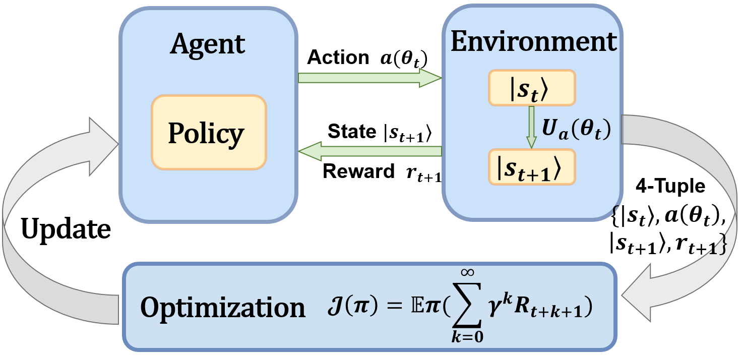
Figure 1: The QRL model. Each iterative step can be described by the following loop: (1) at step $t$, the agent receives $|s_{t}\rangle$ and generates the action parameter $\bm{\theta}_{t}$ according to the current policy; (2) the agent generates $|s_{t+1}\rangle\equiv U_{a}(\bm{\theta}_{t})|s_{t}\rangle$; (3) based on $|s_{t}\rangle$ and $|s_{t+1}\rangle$, a reward $r_{t+1}$ is calculated and fed back to the agent, together with $|s_{t+1}\rangle$; (4) based on $|s_{t+1}\rangle$ and $r_{t+1}$, the policy is updated and then used to generate $\bm{\theta}_{t+1}$.

In artificial intelligence, an agent is a mathematical abstraction representing an object with learning and decision-making abilities. It interacts with its environment, which includes everything except the agent. The core idea of RL is, through the iterative interactions, the agent learns and selects actions, and the environment responds to these actions, by updating its state and feeding it back to the agent. In the meanwhile, the environment also generates rewards, which are some value-functions the agent aims to maximize over its choice of actions along the sequential interactions [1].

Most reinforcement learning problems can be described by a Markov Decision Process (MDP) [37, 1] with basic elements including a set of states $\mathcal{S}$, a set of actions $\mathcal{A}$ and the reward $\mathcal{R}$. The agent interacts with its environment at each of a sequence of discrete time steps, $t=0,1,\cdots,T$. Each sequence like this generated in RL is called an episode. At each time step $t$, the agent receives a representation of the environment’s state, denoted by an $N$-dimensional vector $s_{t}\in\mathcal{S}$, based on which it then chooses an action $a_{t}\in\mathcal{A}$, resulting the change of the environment’s state from $s_{t}$ to $s_{t+1}$. At the next step, the agent receives the reward $r_{t+1}$ determined by the 3-tuple $(s_{t},a_{t},s_{t+1})$. The aim of the agent is to find a policy $\pi$ that maximizes the cumulative reward $R_{t}=\sum_{k=0}^{T}\gamma^{k}r_{t+k+1}$, where $\gamma$ is a discount factor, $0\leq\gamma\leq 1$. A large discount factor $\gamma$ means that the agent cares more about future rewards. The policy can be considered as a mapping from $\mathcal{S}$ to $\mathcal{A}$. The update of the policy $\pi$ is achieved by optimizing the value function $Q(s_{t},a_{t})\equiv E[R_{t}|s_{t},a_{t}]$, i.e., the expectation of $R_{t}$ under the policy $\pi$. Depending on whether the action space is discrete or continuous, the RL problems can be classified into two categories: DAS(discrete action space) and CAS, with different algorithmic design to update the agent’s policy. For DAS problems, popular RL algorithms includes Q-learning [16], Sarsa [38], DQN [18], etc.; for CAS problems, popular algorithms include Policy Gradient [39], DDPG [19], etc.

3 The framework of quantum reinforcement learning

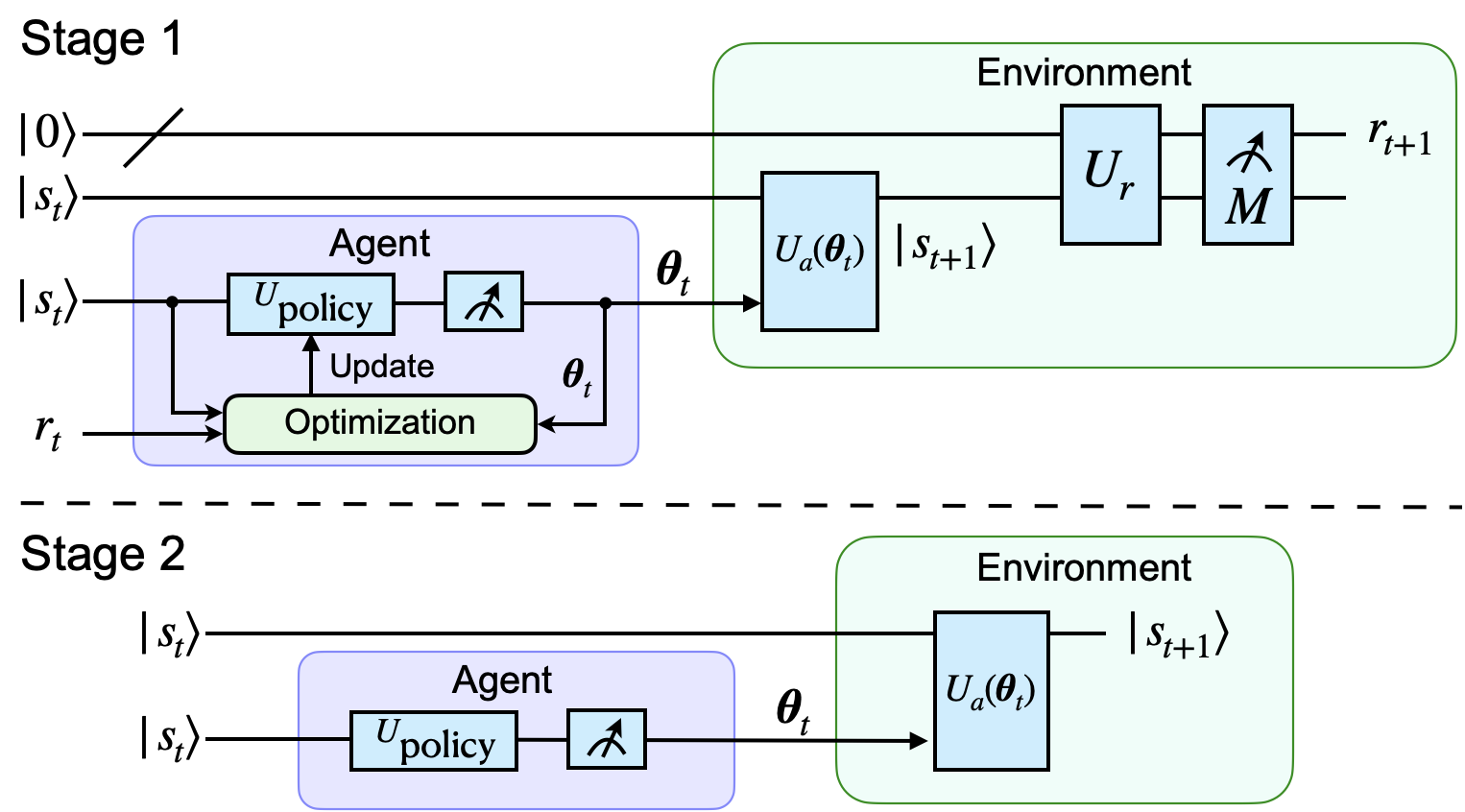
Figure 2: The quantum circuit for our QRL framework at each iteration. The entire QRL process includes two stages, so we give the circuit separately. In stage 1, the circuit includes two registers: the reward register, initialized $|0\rangle$, and the environment register $|s_{t}\rangle$. $U_{\operatorname{policy}}$ is generated by the quantum neural network, and determines the action unitary $U_{a}(\bm{\theta}_{t})$. $U_{r}$ and $M$ are designed to generate the reward $r_{t+1}$. In stage 2, the circuit has only environment register and does not need to feedback the reward value and update the policy.

In order to construct a quantum framework that works for both CAS and DAS cases, we present the following QRL model, as shown in Fig. 1. The essential idea is to map the elements of classical RL into the quantum counterparts. We introduce a quantum ‘environment’ register to represent the environment in RL, and its quantum state $|s_{t}\rangle$ to represent the classical state $s_{t}$ at time step $t$. Then the action $a(\bm{\theta}_{t})$ can be represented as a parameterized action unitary $U_{a}(\bm{\theta}_{t})$ on $|s_{t}\rangle$, where $\bm{\theta}_{t}$ is the action parameter, which is continuous for CAS case, and takes values from a finite set for DAS case. In order to generate the quantum reward function, by introducing a reward register $|r_{t}\rangle$, we design the reward unitary $U_{r}$ and the measurement observable $M$ such that $r_{t+1}\equiv f(\langle s_{t}|\langle 0|U_{a}^{\dagger}(\bm{\theta}_{t})U_{r}^{\dagger}MU_{r}U_{a}(\bm{\theta}_{t})|0\rangle|s_{t}\rangle)$ will match the actual reward defined by the RL problem. Here, $f$ is a function determined by the problem and $|0\rangle$ is the initial state of the reward register. It will be clear in the context of a concrete problem how to design $M$, $U_{r}$, and $f$ in the correct way, which will be discussed in detail based on the quantum state generate problem and the eigenvalue problem in the following.

With all RL elements represented as the components of a quantum circuit shown in Fig. 2, it remains to show how to find the optimal policy $\bm{\theta}_{t}=\bm{\pi}(|s_{t}\rangle)$ at each time step $t$, such that the iterative sequence $U_{\operatorname{tot}}=U_{a}(\bm{\theta}_{T})\cdots U_{a}(\bm{\theta}_{1})U_{a}(\bm{\theta}_{0})$ will drive the arbitrary initial state $|s_{0}\rangle$ converging to the target state $|s_{d}\rangle$. The entire QRL process can be divided into two stages. In stage 1, we construct the optimal policy $U_{\operatorname{policy}}$ through the agent training, including the policy update and the value-function estimation, which can be realized through the function fitting using QNNs. In stage 2, under the established optimal policy, we can iteratively generate the desired sequence $\{U_{a}(\bm{\theta}_{t})\}$ that will drive the initial state to the target state, and complete the RL task.

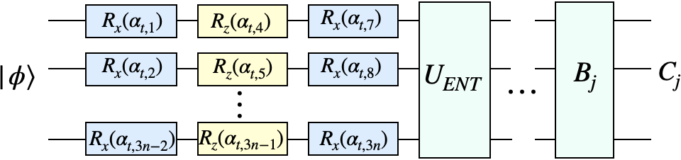
Figure 3: Circuit architecture for the VQC. $R_{\beta}(\alpha)\equiv\exp(-i\sigma_{\beta}\alpha/2)$ with $\beta=x,z$. $U_{\textup{ENT}}\equiv\prod_{k=1}^{n-1}\operatorname{CNOT}_{(k,k+1)}$, where $\operatorname{CNOT}_{(k,k+1)}$ denotes the CNOT gate using the $k$-th qubit to control the $(k+1)$-th qubit. $C_{j}$ is the outcome of the measurement on the observable $B_{j}$, $j=1,2,\cdots$.

In our method, in order to solve RL problems in CAS, we utilize QNNs to construct the policy function and the value function. One popular way of implementing a QNN is to use the variational quantum circuit (VQC) [35, 36, 40, 41], whose parameters can be iteratively optimized for the given objective function on classical computers. The VQC circuit of our quantum DDPG algorithm consists of a sequence of unitary $\{D^{(k)}(\bm{\alpha})\}$, and is ended by measurements of observables $\{B_{j}\}$ with $\operatorname{Tr}(B_{i}B_{j})=0$ (Fig.3), where $B_{j}=b_{j,1}\otimes b_{j,2}\otimes\cdots\otimes b_{j,n}$ and $b_{j,i}\in\{\sigma_{x},\sigma_{y},\sigma_{z},I\}$. Each $D^{(k)}(\bm{\alpha})$ can be chosen to have an identical structure, $D^{(k)}(\bm{\alpha})\equiv U_{\textup{ENT}}V^{(k)}(\bm{\alpha})$, where $V^{(k)}(\bm{\alpha})\equiv\otimes_{l=1}^{n}(R_{x}(\alpha_{k,3l-2})R_{z}(\alpha_{k,3l-1})R_{x}(\alpha_{k,3l}))$, $U_{\textup{ENT}}\equiv\prod_{k=1}^{n-1}\operatorname{CNOT}_{(k,k+1)}$ and $\operatorname{CNOT}_{(k,k+1)}$ uses the $k$-th qubit to control the $(k+1)$-th qubit. Here, $R_{x,z}$ are rotations, with $R_{\beta}(\alpha)\equiv\exp(-i\sigma_{\beta}\alpha/2)$, $\beta=x,z$. For the input $|\phi\rangle$, the output of the VQC can be expressed as the expected measurement outcome $C_{j}\equiv\langle\phi|D^{\dagger}(\bm{\alpha}){B_{j}}D(\bm{\alpha})|\phi\rangle$, based on which the parameter $\bm{\alpha}$ can then be optimized for the given optimization problem, on a classical computer.

4 Quantum DDPG algorithm

For RL problems in CAS, we aim to design QNNs to iteratively construct a sequence of unitary gates that will drive the environment register from the initial state eventually to the target state. This is the essential idea of the quantum DDPG algorithm. Analogous to the classical DDPG algorithm, we make use of the QNNs to construct the desired policy function $\pi_{\bm{\eta}}$ and the value function $Q_{\bm{\omega}}$. Specifically, the policy-QNN is used to approximate the policy function $\theta_{t,j}\equiv\langle s_{t}|D^{\dagger}(\bm{\eta}){B_{j}}D(\bm{\eta})|s_{t}\rangle$ with $\bm{\theta}_{t}=(\theta_{t,1},\theta_{t,2},\dots)$, and the Q-QNN is used to approximate the value function $Q(|s_{t}\rangle,\bm{\theta}_{t})\equiv\langle\bm{\theta}_{t}|\langle s_{t}|D^{\dagger}(\bm{\omega}){B_{Q}}D(\bm{\omega})|s_{t}\rangle|\bm{\theta}_{t}\rangle$. In order to make the training more stable, two more target networks are included with the same structure as the two main networks [3, 18, 19]. Therefore, the quantum DDPG uses four QNNs in total: (1) the policy-QNN $\pi_{\bm{\eta}}(|s_{t}\rangle)$, (2) the Q-QNN $Q_{\bm{\omega}}(|s_{t}\rangle,\bm{\theta}_{t})$, (3) the target-policy $\pi^{\prime}_{\bm{\eta^{\prime}}}(|s_{t}\rangle)$ and (4) the target-Q $Q^{\prime}_{\bm{\omega^{\prime}}}(|s_{t}\rangle,\bm{\theta}_{t})$.

Algorithm 1 Quantum DDPG algorithm

Randomly initialize $Q_{\bm{\omega}}(|s\rangle,\bm{\theta})$ and $\pi_{\bm{\eta}}(|s\rangle)$;

Initialize target $Q^{\prime}$ and $\pi^{\prime}$;

Initialize replay buffer $\bm{D}$;

for episode=1, M do

     Prepare the initial state $|0,s_{0}\rangle$;

     for t=1:$T$ do

         Select the actions: $\bm{\theta}_{t}=\pi_{\bm{\eta}}(|s_{t}\rangle)$;

         Apply $U_{a}(\bm{\theta}_{t})$: $|s_{t+1}\rangle=U_{a}(\bm{\theta}_{t})|s_{t}\rangle$;

         Apply $U_{r}$ and $M$ to obtain $r_{t+1}$;

         Store tuple $(|s_{t}\rangle,\bm{\theta}_{t},r_{t},|s_{t+1}\rangle)$ in $\bm{D}$;

         Sample a batch of tuples $(|s_{i}\rangle,\bm{\theta}_{i},r_{i},|s_{i+1}\rangle)$ from $\bm{D}$;

         Set $y_{i}=r_{i}+\bm{\gamma}Q^{\prime}_{\bm{\omega}^{\prime}}(|s_{i+1}\rangle,\pi^{\prime}_{\bm{\eta}^{\prime}}(|s_{i+1}\rangle))$;

         Update Q-QNN by minimizing the loss:

         $L=\frac{1}{G}\sum_{i}(y_{i}-Q_{\bm{\omega}}(|s_{i}\rangle,\bm{\theta}_{i}))^{2}$;

         Update the policy-QNN:

         $\nabla_{\bm{\eta}}J\approx\frac{1}{G}\sum_{i}\nabla_{\bm{\theta}}Q_{\bm{\omega}}(|s_{i}\rangle,\bm{\theta_{i}})\nabla_{\bm{\eta}}\pi_{\bm{\eta}}(|s_{i}\rangle)$;

         Update the target QNNs:

         $\bm{\omega}^{\prime}\leftarrow\tau\bm{\omega}+(1-\tau)\bm{\omega}^{\prime};\bm{\eta}^{\prime}\leftarrow\tau\bm{\eta}+(1-\tau)\bm{\eta}^{\prime}$.

     end for

end for

The quantum DDPG method contains two stages. In stage 1, the agent training is divided into three parts: (1) experience replay [42], (2) updates of the Q-QNN and the policy-QNN, and (3) updates of the target networks. The aim of the experience replay is to prevent the neural network from overfitting. We store the agent’s experiences $(|s_{t}\rangle,\bm{\theta}_{t},r_{t},|s_{t+1}\rangle)$ in a finite-sized replay buffer $\bm{D}$ at each time step. During the training, we randomly sample a batch of experiences from the replay buffer to update the Q-QNN and the policy-QNN. First, we update the policy-QNN parameters by minimizing the expected return $J=E[Q_{\bm{\omega}}(|s\rangle,\bm{\theta})|_{|s\rangle=|s_{i}\rangle,\bm{\theta}=\pi(|s_{i}\rangle)}]$. Then we update the Q-QNN parameters by minimizing the mean-squared loss $L=\frac{1}{G}\sum_{i}(y_{i}-Q_{\bm{\omega}}(|s_{i}\rangle,\bm{\theta}_{i}))^{2}$ between the predicted Q-value and the original Q-value, where $y_{i}=r_{i}+\bm{\gamma}Q^{\prime}_{\bm{\omega}^{\prime}}(|s_{i+1}\rangle,\pi^{\prime}_{\bm{\eta}^{\prime}}(|s_{i+1}\rangle))$ is the predicted Q-value and calculated by the target-Q networks, $G$ is the size of the batch. Here, we use the gradient descent algorithm AdamOptimizer [43] to minimize the loss function of these two quantum neural networks. Finally, we update the two target networks using a soft update strategy [19]: $\bm{\omega}^{\prime}\leftarrow\tau\bm{\omega}+(1-\tau)\bm{\omega}^{\prime}$, $\bm{\eta}^{\prime}\leftarrow\tau\bm{\eta}+(1-\tau)\bm{\eta}^{\prime}$, where $\tau$ is a parameter with $0<\tau<1$. The entire training process is summarized in Algorithm 1. In stage 2, with the optimal policy-QNN and $T$ iterations, we can construct a sequence of $\{U_{a}(\bm{\theta}_{t})\}$ and $|s_{t}\rangle$ for each given initial $|s_{0}\rangle$, satisfying $|s_{T}\rangle$ is sufficiently close to the target $|s_{d}\rangle$.

For DAS problems, the above QRL proposal still works if the quantum DDPG design in Fig. 2 is replaced by the quantum DQN design, analogous to the classical DQN algorithm [18]. Compared with the quantum DDPG, the quantum DQN maps states of the environment into the computational basis, rather than into the amplitudes of a quantum register. Moreover, for quantum DQN, only the value function needs to be approximated by the QNN, while the policy function can be described by the greedy algorithm [1]. Detailed proposals to solve DAS problems using QNNs are presented in [40, 44]. It is worthwhile to note that the quantum DQN cannot efficiently solve CAS problems, since the dimensionality problem is inevitable when solving the CAS problems through discretization.

5 Quantum DDPG in solving quantum state generation problems

The quantum state generation problem is a very important ingredient in quantum computation and quantum control. Given a target state $|s_{d}\rangle$, we hope to find a sequence of unitary operations $\{U_{a}(\bm{\theta}_{t})\}$ that can drive the quantum system from the initial state $|s_{0}\rangle$ to $|s_{d}\rangle$. In conventional quantum control algorithms, the desired control sequence $\{U_{a}(\bm{\theta}_{t})\}$ can be found through optimization; if a different target state $|s_{d}\rangle$ is chosen, a new optimization is required to find the desired control sequence for the new $|s_{d}\rangle$. In other words, $\{U_{a}(\bm{\theta}_{t})\}$ are generated through optimization case by case for different target $|s_{d}\rangle$. Now, we try to solve the same problem through our QRL algorithm: in the language of RL, we aim to find the optimal policy $U_{\operatorname{policy}}$ so that arbitrary initial state $|s_{0}\rangle$ can be iteratively driven to the given target state $|s_{d}\rangle$ by applying a sequence of $\{U_{a}(\bm{\theta}_{t})\}$ generated by $U_{\operatorname{policy}}$. Compared with the traditional method, the advantage of our method is that it only involves a one-shot optimization to construct the QRL model and there is no need to optimize case by case for different $|s_{d}\rangle$.

The QRL circuit for arbitrary state generation is shown in Fig. 2. First, we define the environment $U_{r}$, and at each step $t$, we define the reward function $r_{t+1}=f(p_{t+1})$. Given the target $|s_{d}\rangle$, we choose an observable $M_{d}\equiv|s_{d}\rangle\langle s_{d}|$. Then we can obtain an estimate of $p_{t+1}\equiv\langle M_{d}\rangle=\langle s_{t+1}|M_{d}|s_{t+1}\rangle$ through the measurement statistics of $M_{d}$, with estimation error $\epsilon$. Notice that the number of measurements required to obtain $p_{t+1}$ and $r_{t+1}=f(p_{t+1})$ is independent of the system size $N=2^{n}$ of the $n$-qubit environment register, and the proof will be shown later in the following. Let $|s_{0}\rangle=\sum_{k=1}^{N}\alpha_{0,k}|v_{k}\rangle$ be the initial state of the environment register, where $\alpha_{0,k}=\langle v_{k}|s_{0}\rangle$. At time step $t$, applying $U_{\operatorname{policy}}$ and quantum measurements on $|s_{t}\rangle$, as shown in Fig. 2, we obtain the action parameter $\bm{\theta}_{t}$, and generate the corresponding action unitary $U_{a}(\bm{\theta}_{t})\equiv U_{\textup{ENT}}V(\bm{\theta}_{t})$, where $V(\bm{\theta}_{t})$ and $U_{\textup{ENT}}$ are defined as in Fig. 3. Then we apply $U_{a}(\bm{\theta}_{t})$ and get

$$|s_{t+1}\rangle=U_{a}(\bm{\theta}_{t})|s_{t}\rangle=U_{\textup{ENT}}V(\bm{\theta}_{t})|s_{t}\rangle.$$ (1)

Next, by measuring $M_{d}$, we obtain an estimation of

$$p_{t+1}\equiv\langle s_{t+1}|M_{d}|s_{t+1}\rangle=|\langle s_{t+1}|s_{d}\rangle|^{2}$$ (2)

through $K$ number of measurements. For this state generation problem, we choose the reward $r_{t+1}=10p_{t+1}$. If $p_{t+1}\to 1$ as $t\to\infty$, then $|s_{t+1}\rangle$ will converge to $|s_{d}\rangle$ to complete the RL goal. Notice that the evaluation of $r_{t+1}$ is only needed for the QRL training stage; in the application stage, since $U_{\operatorname{policy}}$ is optimized, measurements are no longer required to estimate $r_{t+1}$. Then by implementing stage 1 and stage 2 of our method, the state generation problem will be solved with our quantum DDPG algorithm.

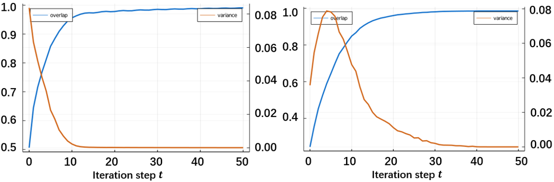
Figure 4: Simulation results for quantum state generation problem of the one-qubit and the two-qubit Hamiltonian by quantum DDPG. For $1000$ different initial $|s_{0}\rangle$, we plot how the average $\bar{p}_{t}$ and the variance $\Delta(p_{t})$ change with the iteration step $t$. For the one-qubit case, at $t=50$, $\bar{p}_{50}\geq 0.99$ and $\Delta(p_{50})\leq 4.47\times 10^{-5}$. For the two-qubit case, at $t=50$, $\bar{p}_{50}\geq 0.98$ and $\Delta(p_{50})\leq 4.04\times 10^{-7}$.

To verify the effectiveness of our method, we study the state generation problem for one-qubit and two-qubit cases. In stage 1, we apply the quantum DDPG algorithm to update the policy until we obtain the optimal $U_{\operatorname{policy}}$. Since the interaction between agent and environment is influenced by noise, we randomly choose the error $\epsilon\sim\mathcal{N}(p_{t},\epsilon^{2})$ on the reward value in the simulation. In stage 2, based on $U_{\operatorname{policy}}$ and $|s_{0}\rangle$, we generate a sequence of $\{U_{a}(\bm{\theta}_{t})\}$ and the corresponding $|s_{50}\rangle=U_{a}^{\dagger}(\bm{\theta}_{49})\cdots U_{a}^{\dagger}(\bm{\theta}_{0})|s_{0}\rangle$, and record the overlap $p_{t}$ at each $t$.

Specifically, for the one-qubit case, the target state is chosen to be $|1\rangle$. In stage 1, the size of the replay buffer is set as $1000$, the size of the batch is set as $16$, and the other parameters are set as $\gamma=0.9$, $\tau=0.001$. In addition, the quantum registers for the policy-QNN and the value-QNN are both comprised of three qubits, and the depth of the QNN circuits is one. For the policy-QNN, we add two ancilla qubits initialized in $|00\rangle$ together with $|s_{t}\rangle$ as the input of the policy network. For the value-QNN, we encode $\bm{\theta}_{t}$ into $|\bm{\theta}_{t}\rangle$ and use it together with $|s_{t}\rangle$ as the inputs of the value-QNN. Then we perform the training process. After the training stage, we randomly select 1000 different initial states $|s_{0}\rangle$ to test the performance of the policy $U_{\operatorname{policy}}$. In Fig. 4, we can see that almost all final states $|s_{50}\rangle$ are sufficiently close to the target $|s_{d}\rangle$, with $p_{50}\geq 0.99$ and $\Delta(p_{50})\leq 4.67\times 10^{-5}$ at $t=50$. For the two-qubit case, the target state $|s_{d}\rangle$ is chosen to be the maximum entangled state $(|00\rangle+|11\rangle)/\sqrt{2}$. In order to improve the training performance, we apply the quantum neural network proposed in Ref. [45], which introduced a classical activation function and a weight matrix on the basis of VQC. Also, we set the size of the replay buffer as $10000$, the size of the batch as $128$, and other parameters as $\gamma=0.9$, $\tau=0.005$. Here, the quantum registers to implement these two QNNs both contain six qubits, and the depth of both QNN circuits is three. Simulation results in Fig. 4 show that $\bar{p}_{50}\geq 0.98$ and $\Delta(p_{50})\leq 4.04\times 10^{-7}$ at $t=50$. Notice that for both one-qubit and two-qubit cases, a one-shot optimization is sufficient to find the optimal policy $U_{\operatorname{policy}}$ through QNN learning. Once the QRL model is constructed, for each $|s_{0}\rangle$, it can efficiently generate the desired control sequence $\{U_{a}(\bm{\theta}_{t})\}_{t=0}^{49}$ to drive $|s_{0}\rangle$ to $|s_{d}\rangle$. If we take $|s_{d}\rangle$ as the initial state, then the reversed sequence $\{U_{a}^{\dagger}(\bm{\theta}_{t})\}_{t=49}^{0}$ will drive $|s_{d}\rangle$ to arbitrary $|s_{0}\rangle$. Thus, we have completed the task of arbitrary state generation. It is worthwhile to note that it is not necessary for $|s_{0}\rangle$ to be known to make our model work: even if $|s_{0}\rangle$ is unknown, as long as we have sufficient number of identical copies of $|s_{0}\rangle$, our model is still able to output the desired sequence that will drive $|s_{d}\rangle$ to $|s_{0}\rangle$. Hence, our model can also be used to physically reconstruct an unknown state.

6 Quantum DDPG in solving the eigenvalue problem

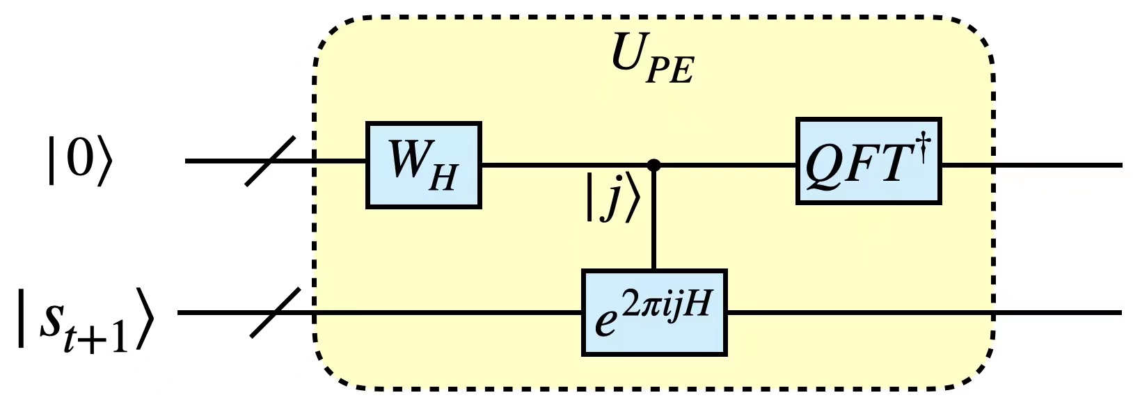
Figure 5: The quantum phase estimation circuit $U_{\operatorname{PE}}$.

In quantum complexity theory, the Quantum Merlin Arthur(QMA) is the set of all decision problems that can be verified by quantum computers in polynomial time [46, 47, 48]. One typical QMA-complete problem is the $k$-local Hamiltonian problem, which is to find the ground energy of a $k$-local Hamiltonian $H$ with $k\geq 2$ [49]. Essentially, this problem is an eigenvalue problem for a given physical Hamiltonian, and one way of solving it on a quantum computer is to use the variational quantum eigensolver (VQE) algorithm [35]. Here, we present an alternative method, formulating the $k$-local Hamiltonian problem as a reinforcement learning problem in CAS and applying our quantum DDPG algorithm to it. Specifically, let $H$ be the Hamiltonian defined on $N$ dimensional quantum system $E$, and $H$ is a sparse matrix that can be efficiently constructed. Assuming an unknown eigenvalue $\lambda_{0}$ of $H$ is located in a neighborhood of $\bar{\lambda}$, i.e. $\lambda_{0}\in\delta(\bar{\lambda})\equiv[\bar{\lambda}-\delta,\bar{\lambda}+\delta]$, we aim to find out $\lambda_{0}$ and its corresponding eigenvector $|u_{0}\rangle$. To implement the QRL circuit in Fig. 2 for the eigenvalue problem, we choose $U_{r}$ as the quantum phase estimation $U_{\operatorname{PE}}$ shown in Fig. 5. The role of $U_{\operatorname{PE}}$ together with the subsequent measurement is to map the input state $|s_{t+1}\rangle$ into the desired eigenstate with certain probability. Specifically, the reward function $r_{t+1}$ can be defined as the overlap between the $(t+1)$-th states with $|u_{0}\rangle$: $r_{t+1}\equiv 10|\langle s_{t+1}|u_{0}\rangle|^{2}$. Let $|0\rangle$ and $|s_{0}\rangle=\sum_{k=1}^{N}\alpha_{0,k}|u_{k}\rangle$ be the initial states of the reward register and the $n$-qubit environment register, where $n=\log N$ and $\alpha_{0,k}=\langle u_{k}|s_{0}\rangle$. At the time step $t$, applying $U_{\operatorname{policy}}$ and quantum measurements to $|s_{t}\rangle$, we obtain the action parameter $\bm{\theta}_{t}$, and the next state is $|s_{t+1}\rangle=U_{a}(\bm{\theta}_{t})|s_{t}\rangle$. Then, by applying $U_{\operatorname{PE}}$, we obtain

$$U_{\operatorname{PE}}|0\rangle|s_{t+1}\rangle=\sum_{k=1}^{N}\alpha_{t+1,k}|{\lambda}_{k}\rangle|u_{k}\rangle,$$ (3)

where $|u_{k}\rangle$ is the eigenvector corresponding to the eigenvalue $\lambda_{k}$. By measuring the eigenvalue phase register, we obtain the outcome $\lambda_{0}$ with probability

$$p_{t+1}\equiv|\langle s_{t+1}|u_{0}\rangle|^{2}=|\alpha_{t+1,0}|^{2}$$ (4)

which can be estimated by the frequency of obtaining $\lambda_{0}$ in $K$ number of measurements. The reward can be written as $r_{t+1}=10p_{t+1}$.

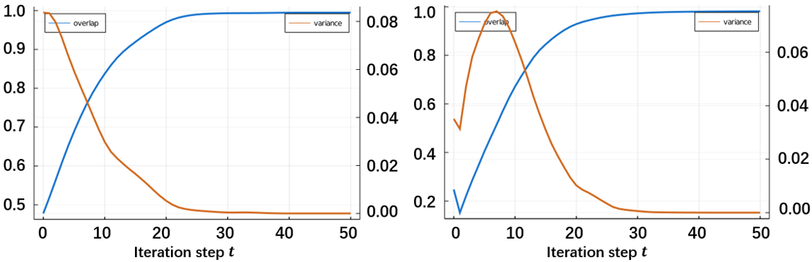
Figure 6: Simulation results for solving the eigenvalue problem of the one-qubit and the two-qubit Hamiltonian by quantum DDPG. For $1000$ different initial $|s_{0}\rangle$, we plot how the average $\bar{p}_{t}$ and the variance $\Delta(p_{t})$ change with the iteration step $t$. For the one-qubit case, at $t=50$, $\bar{p}_{50}\geq 0.99$ and $\Delta(p_{50})\leq 1.98\times 10^{-7}$. For the two-qubit case, at $t=50$, $\bar{p}_{50}\geq 0.98$ and $\Delta(p_{50})\leq 3.01\times 10^{-6}$.

Next, as numerical demonstration, we apply this method to the Heisenberg model with $n=1,2$. In stage 1, the parameter settings of the quantum neural networks are the same as in the cases of $n=1,2$ in the state generation problem. After the training in stage 1, we randomly select 1000 different initial states $|s_{0}\rangle$ to test the policy $U_{\operatorname{policy}}$. For the one-qubit case, we choose the Hamiltonian as $H\equiv\frac{1}{4}(0.13\sigma_{x}+0.28\sigma_{y}+0.95\sigma_{z}+I)$, where the three coupling constants are randomly generated. One can see from Fig. 6 that as $t$ increases, trajectories $\{|s_{t}\rangle\}$ with different initial $|s_{0}\rangle$ all converge to the ground state $|u_{0}\rangle$, with $\bar{p}_{50}\geq 0.99$ and $\Delta({p_{50}})\leq 1.98\times 10^{-7}$ at $t=50$. Next, we consider a two-qubit Hamiltonian model $H=\frac{1}{2}(\sigma_{x}\otimes\sigma_{x}+\sigma_{y}\otimes\sigma_{y}+\sigma_{z}\otimes\sigma_{z})+0.25\sigma_{x}\otimes I$, and use the quantum DDPG algorithm to find an energy state of it. The simulation result is shown in Fig. 6 that as $t$ increases, trajectories with different initial $|s_{0}\rangle$ all converge to the ground state of $H$, with $\bar{p}_{50}\geq 0.98$ and $\Delta({p_{50}})\leq 3.01\times 10^{-6}$ at $t=50$. However, we are not satisfied with the accuracy rate of 0.98, so we can use the final state $|s_{50}\rangle$ as the input of the method of Ref. [50] to obtain an exact state.

Again, analogous to the state generation problem, our QRL method demonstrates an advantage over the conventional optimal control [51] or the VQE [35] algorithms: the optimal $U_{\operatorname{policy}}$ generated through a one-shot optimization is useful for arbitrary initial state, while a different optimization is required for each different initial state in optimal control or VQE.

7 Complexity analysis

Analogous to the VQE algorithm, our quantum DDPG algorithm is essentially a quantum-classical hybrid optimization. Similar to other discussion, we will mainly focus on the quantum circuit complexity of our algorithm, including the circuit gate complexity and the measurement complexity. In our method, quantum measurements are required to obtain both the reward value and the action parameters.

Let $B$ be an observable with $B|u_{j}\rangle=\lambda_{j}|u_{j}\rangle$, for an $n$-qubit system, $N=2^{n}$. Assuming the system is in the state $|\psi\rangle=\sum_{j=1}^{N}\alpha_{j}|u_{j}\rangle$, the measurement of $B$ in $|\psi\rangle$ will generate the measurement outcome $m$, with probability distribution $P(m=\lambda_{j})=|\langle u_{j}|\psi\rangle|^{2}=|\alpha_{j}|^{2}$. Notice that $m$ and $B$ have the same expectation value and the variance: $\mathbb{E}(m)=\langle B\rangle$ and $\text{Var}(m)=\langle B^{2}\rangle-\langle B\rangle^{2}$. Then we have the following well-known result in probability theory:

Lemma 1 (Chebyshev’s inequality).

Let $X$ is a random variable with expected value $\mu$ and variance $\sigma^{2}$. For any real number $k>0$, $P(|X-\mu|\geq k\sigma)\leq\frac{1}{k^{2}}$.

Based on Lemma $1$, we further derive the following relationship between the measurement precision error $\epsilon$ and the number of measurements $K$ to reach that precision.

Theorem 1.

Let $B$ be an observable with $B=b_{1}\otimes b_{2}\otimes\cdots\otimes b_{n}$, where $b_{i}\in\{\sigma_{x},\sigma_{y},\sigma_{z},I\}$. We implemented measurements for $K$ times to obtain the sample average $\overline{m}_{K}$ to estimate the expected value $\langle B\rangle$. Then, the probability of the difference between $\overline{m}_{K}$ and $\langle B\rangle$ lager than $\epsilon$ is given by

$$P(|\overline{m}_{K}-\langle B\rangle|\geq\epsilon)\leq\frac{1}{K\epsilon^{2}}.$$ (5)

Proof.

After $K$ number of measurements on $B$, we obtain a sample of measurement outcomes, $m_{1},m_{2},\cdots,m_{K}$, with sample mean $\overline{m}_{K}\equiv\frac{1}{n}\sum_{i=1}^{K}m_{i}$ and $\{m_{i}\}$ to be independent and identically distributed. Let the expectation and the variance of $m_{i}$ be $\mu$ and $\sigma^{2}$. Due to the weak law of large numbers, we have $\overline{m}_{K}\to\mu$ for $n\to\infty$. Then the expectation of the sample mean is $\mathbb{E}(\overline{m}_{K})=\mu=\langle B\rangle$ and the variance is $\text{Var}(\overline{m}_{K})=\frac{\sigma^{2}}{K}$. Choosing $\epsilon=k\frac{\sigma}{\sqrt{K}}$ and using Chebyshev’s inequality result in $P(|\overline{m}_{K}-\langle B\rangle|\geq\epsilon)\leq\frac{\sigma^{2}}{K\epsilon^{2}}$.

For the observable $B=b_{1}\otimes b_{2}\otimes\cdots\otimes b_{n}$ and $b_{i}\in\{\sigma_{x},\sigma_{y},\sigma_{z},I\}$, we have $\lambda_{i}=\pm 1$ and $\langle B^{2}\rangle$ is $1$. Further, we have $0\leq\langle B\rangle^{2}\leq 1$ and $0\leq\langle B^{2}\rangle-\langle B\rangle^{2}\leq 1$. Hence, $0\leq\sigma\leq 1$, and we find $P(|\overline{m}_{K}-\langle B\rangle|\geq\epsilon)\leq\frac{1}{K\epsilon^{2}}$. ∎

Now we apply Theorem 1 to analyze the measurement complexity of our algorithm. For a given estimation error $\epsilon$, according to Theorem 1, choosing $K=\mathcal{O}(\frac{1}{\epsilon^{2}})$ will make $\overline{m}_{K}$ converge to $\langle B\rangle$ with high probability. Next, we analyze the gate complexity of our algorithm. During a single iteration at $t$ of stage 1, denoting the gate complexities of $U_{a}(\bm{\theta_{t}})$, $U_{\operatorname{policy}}$(policy-QNN) and $U_{Q}$(Q-QNN) as $C_{a}$, $C_{p}$ and $C_{q}$, we can see that the number of parameters $\bm{\theta_{t}}$ in $U_{a}(\bm{\theta_{t}})$ is at most equal to $C_{a}$. Hence, in a single iteration at $t$ of stage 1, the gate complexity is $\mathcal{O}(\frac{C_{a}C_{p}+C_{a}^{2}t+C_{q}}{\epsilon^{2}})$. Analogously, in a single iteration at $t$ of stage 2, the gate complexity is $\mathcal{O}(C_{a}t)+\mathcal{O}(\frac{C_{p}+C_{a}t}{\epsilon^{2}}C_{a})$; hence, the total gate complexity of stage 2 is $\mathcal{O}(\frac{T^{2}C_{a}^{2}+C_{a}C_{p}}{\epsilon^{2}})$.

8 Concluding discussion

In this work, inspired by the classical DDPG algorithm, we have proposed a quantum DDPG algorithm that can solve both CAS and DAS reinforcement learning problems. For CAS tasks, our quantum DDPG algorithm encodes the environment state into the quantum state amplitude to avoid the dimensionality disaster due to discretization. As a useful application, our method can be used to solve the state generation problem. A distinguishing feature of our method is that, for each target state, it only requires a one-shot optimization to construct the QRL model that is able to efficiently output the desired control sequence driving the initial state to the target state. In comparison, in conventional quantum control methods, different optimizations are required for each different target state. Simulation results for one-qubit and two-qubit quantum systems demonstrate that, our QRL method can be used for arbitrary state generation and eigenstate preparation for a given Hamiltonian. We have also analyzed the complexity of our proposal in terms of the QNN circuit complexity and the measurement complexity.

Appendix A Classical Reinforcement Learning

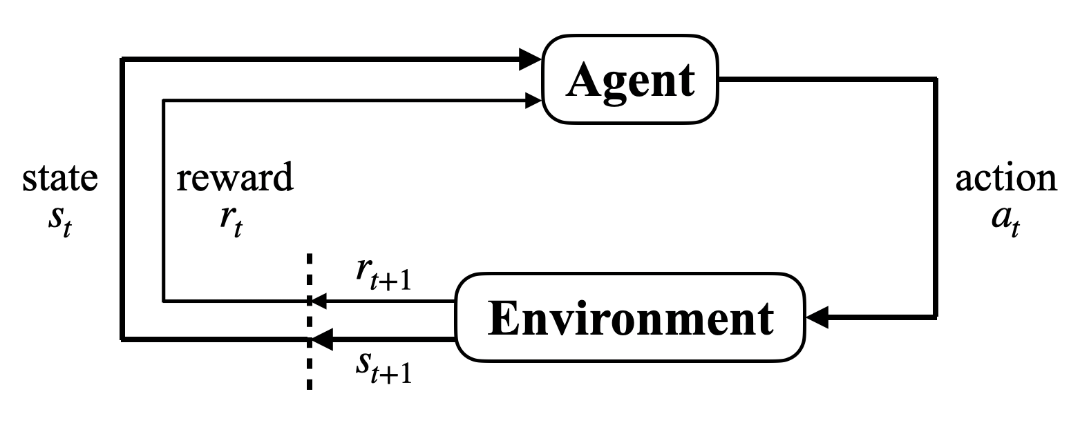
Figure 7: An illustration of the standard RL method.

Here, we will give a detailed introduction to the basic concepts of reinforcement learning for beginners to learn. In RL, the basic elements include a set of states $\mathcal{S}$, a set of actions $\mathcal{A}$, the reward $\mathcal{R}$. The model of reinforcement learning is shown in Fig. 7 [1], the agent and the environment interact continually. In a step, the agent receives an observation $s_{t}$, then chooses an action $a_{t}$. Next, the agent performs an action $a_{t}$, and the environment move to next state $s_{t+1}$ and emits a reward $r_{t+1}$. At the next step, the agent receives the reward $r_{t+1}$ determined by the 3-tuple $(s_{t},a_{t},s_{t+1})$. Given an initial state $s_{0}$, the agent-environment interactions will generate the following sequence: $s_{0},a_{0},r_{1},s_{1},a_{1},r_{2},\cdots$. Such a sequence is called an episode in RL. Next, we define the following three key elements of RL:

(1) Policy

The policy can be considered as a mapping from $\mathcal{S}$ to $\mathcal{A}$, which sets the rules on how to choose the action based on the environment’s state. Such policy is determined by certain optimization objective, such as maximizing the cumulative reward. A policy can be either deterministic or stochastic. A deterministic policy is characterized by a function $a=\pi(s)$, meaning that under the same policy, at time step $t$, the action $a_{t}$ is uniquely determined by the current environment’s state $s_{t}$. Given the state $s$, we define the stochastic policy, $\pi_{\theta}(a|s)\equiv P[a|s,\theta]$ as the probability of choosing the random action $a$, where $\theta$ is parameter charactering the distribution of $P[a|s,\theta]$.

(2) Cumulative reward

As mentioned above, at time step $t$, the policy goal of the agent is to maximize the cumulative reward it receives in the long run. At each step $t$, if we define the accumulative reward as $R_{t}=\sum_{k=0}^{\infty}r_{t+k+1}$, it may not be convergent and becomes ill-defined; alternatively, we can introduce a discount factor $\gamma(0\leq\bm{\gamma}\leq 1)$ and define the cumulative reward as $R_{t}=\sum_{k=0}^{\infty}\gamma^{k}r_{t+k+1}$. The larger the discount factor, the longer time span of future rewards we will consider to determine the current-state policy. At time step $t$, the reward $r_{t}$ determines the immediate return, and the cumulative reward $R_{t}$ determines the long-term return.

(3) Value function

Notice that when $a_{t}$ or $s_{t}$ is stochastic, $r_{t}$ and $R_{t}$ are also stochastic. Hence, we further define the value function $Q$ to be the expectation of the cumulative reward, $Q(s,a)\equiv E[R_{t}|s,a]$, under the policy $\pi$. The goal of RL is to find the optimal policy that maximizes the value function $Q$.

RL problems can be classified into two categories: discrete-action-space(DAS) problems and continuous-action-space (CAS) problems. In a DAS problem, the agent chooses the action from a finite set $\{a_{k}\}$, $k=1,\cdots,l$. For example, in the Pong game [18], the action set for moving the paddle is {up, down}. In a CAS problem, the action can be parametrized as a real-valued vector[52]. In the CartPole environment [53], the action is the thrust and can be parametrized as a continuous variable $\theta\in[-1,1]$. For DAS problems, popular RL algorithms include Q-learning [16], Sarsa [38], Deep Q-learning Network(DQN) [18], etc.; for CAS problems, popular algorithms include Policy Gradient [39], Deep Deterministic Policy Gradient(DDPG) [19], etc.

Notice that the DQN algorithm is only efficient when solving problems with small DAS. It quickly becomes inefficient and intractable when the size of the DAS becomes large. Hence, although a CAS problem can be converted into a DAS problem through discretization, the DQN algorithm will not work in solving the converted DAS problem, if we require high discretization accuracy. For CAS problems, it is better to use a CAS algorithm, such as DDPG.

Appendix B Discrete Action Space Algorithms

Q-learning is a milestone in reinforcement learning algorithms. The main idea of the algorithm is to construct a Q-table of state-action pairs to store the Q-values, and then the agent chooses the action that can obtain the largest cumulative reward based on the Q-values.

In the Q-learning algorithm, an immediate reward matrix $R$ can be constructed to represent the reward value from state $s_{t}$ to the next state $s_{t+1}$. The Q-value is calculated based on the matrix $R$, and it is updated by the following formula [1]:

$$\begin{split}Q(s_{t},a_{t})&\longleftarrow Q(s_{t},a_{t})\\ &+\alpha[r_{t}+\bm{\gamma}\max_{a_{t+1}}Q(s_{t+1},a_{t+1})-Q(s_{t},a_{t})]\end{split}$$ (6)

where $\bm{\gamma}$ is the discount factor, $\alpha$ is the learning rate that determines how much the newly learned value of $Q$ will override the old value. By training the agent, the Q-value will gradually converge to the optimal Q-value.

The Q-learning is only suitable for storing action-state pairs which are low-dimensional and discrete. In large-space tasks, the corresponding Q-table could become extremely large, causing the RL problem intractable to solve, which is known as the curse of dimensionality. The DQN algorithm takes the advantage of deep learning technique to solve the RL problems. Specifically, it introduces a neural network defined as Q-network $Q(s_{t},a_{t};\bm{\omega})$, whose function is similar to the Q-table in approximating the value function. The input of the Q-network is the current state $s_{t}$, and the output is the Q-value. The $\epsilon$-greedy strategy is used to choose the value of $a$ according to the following probability distribution [1]:

$$a=\begin{cases}\arg\max_{a}Q(a),&\text{ with probability}\ 1-\epsilon;\\ \text{a random action},\,&\text{ with probability}\ \epsilon.\end{cases}$$ (7)

In order to stabilize the training, the DQN algorithm uses two tricks: experience replay and a target network. The method of experience replay is to use a replay buffer to store the experienced data and to sample some data from the replay buffer at each step $t$ to update the parameters in the neural network. The DQN algorithm introduces a target-Q network $Q(s_{t+1},a_{t+1};{\bm{\omega}}^{\prime})$ which is a copy of the Q-network. The input of $Q(s_{t+1},a_{t+1};{\bm{\omega}}^{\prime})$ is $s_{t+1}$ and the output is $Q(s_{t+1},a_{t+1})$. However, the target-Q network parameters are updated using Q-network parameters at every $m$ steps, where $m$ is a constant. The DQN algorithm updates the Q-network by reducing the value of the loss function $L(\bm{\omega})=E[((r_{t}+\bm{\gamma}\max_{a_{t+1}}Q^{\prime}(s_{t+1},a_{t+1};{\bm{\omega}}^{\prime}))-Q(s_{t},a_{t};\bm{\omega}))^{2}]$.

Appendix C Continuous Action Space Algorithms

For tasks in continuous action space, we usually use the DDPG algorithm. The DDPG algorithm make use of the neural network to construct the desired policy function $\pi:\,s_{t}\to a_{t}$ such that the value function is maximized. The quantum DDPG includes four neural networks: the policy-network, the Q-network, the target-policy-network and the target-Q-network. The Q-network is used to approximate the value function, while the policy-network is used to approximate the policy function.

The DDPG algorithm uses the same tricks as DQN to stabilize the training. The update of the policy-network is achieved by reducing the loss function $L(\bm{\eta})=-Q(s_{t},a_{t};\bm{\eta})$. Similar to DQN, the update of the Q-network in DDPG is achieved through reducing the value of the loss function $L(\bm{\omega})=E[((r_{t}+\bm{\gamma}\max_{a_{t+1}}Q^{\prime}(s_{t+1},a_{t+1};{\bm{\omega}}^{\prime}))-Q(s_{t},a_{t};\bm{\omega}))^{2}]$. Through training, the estimated value output of the Q-network will be more accurate, and the action given by the policy-network will make the Q-value higher.

Appendix D Quantum Reinforcement Learning in Discrete Action Space

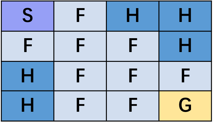
Figure 8: Frozen Lake environment model. S is the starting position; F is the walkable position; H is the hole position, and G is the goal position. The actions that the agent can choose at each position are up, down, left, and right.

Besides DAS problems, our QRL framework can solve DAS problems as well. For DAS tasks, we can use quantum Q-learning or quantum DQN algorithm. Specifically, we consider a Frozen Lake environment model [54] in which both the action space and the state space are finite dimensional, as shown in Fig. 8. In this environment, the agent can move from a grid to its neighboring grids and the goal is to move from the starting position to the target position. Some positions of the grids are walkable, while the others will make the agent fall into the water, resulting in a large negative reward, and a termination of the episode.

In order to solve the Frozen Lake problem using our QRL framework, we number the $N$ grids from $0$ to $N-1$, and encode them into the set of basis states $S=\{|j\rangle\}$, $j=0,\cdots,j-1$ of an $N$-dimensional quantum environment, composed of $n=\log N$ qubits. At each step $t$, the state of the environment $|s_{t}\rangle$ equals to one of the basis states in $S$. The action $a(\bm{\theta}_{t})$ can be represented as a parameterized action unitary $U_{a}(\bm{\theta}_{t})$ on $|s_{t}\rangle$, where $\bm{\theta}_{t}$ is the action parameter. Assuming that at the position $|j\rangle$, there are four actions(up, down, left, and right) the agent can choose from, corresponding to the discrete set $\{U_{a}(\bm{\theta}_{j,k})\}=\{U_{a}(\bm{\theta}_{j,1}),U_{a}(\bm{\theta}_{j,2}),U_{a}(\bm{\theta}_{j,3}),U_{a}(\bm{\theta}_{j,4})\}$ where $\bm{\theta}_{j,k}=(\theta_{j,k}^{(1)},\cdots,\theta_{j,k}^{(n)})^{T}$ is a real vector. Specifically, we construct $U_{a}(\bm{\theta}_{j,k})$ as $U_{a}(\bm{\theta}_{j,k})\equiv R_{y}(\theta_{j,k}^{(1)})\otimes\dots\otimes R_{y}(\theta_{j,k}^{(n)})$, where $R_{y}(\theta_{j,k}^{(n)})=\exp(-i\theta_{j,k}^{(n)}\sigma_{y}/2)$, and $\theta^{(j)}_{k,n}\in\{0,\pi\}$. For example, in Fig. 8, if the agent is at the position $|5\rangle$ and wants to move right to the position $|6\rangle$, then the required action parameter is $\bm{\theta}_{5,4}=(0,0,\pi,\pi)$, corresponding to $U(\bm{\theta}_{5,4})\equiv R_{y}(0)\otimes R_{y}(0)\otimes R_{y}(\pi)\otimes R_{y}(\pi)$, satisfying $U(\bm{\theta}_{5,4})|0101\rangle=|0110\rangle$.

We generate the reward function $f$ by introducing a reward register $|r_{t}\rangle$ and design the reward unitary $U_{r}=\sum_{j\in F}|j\rangle\langle j|\otimes I\otimes I+\sum_{j\in H}|j\rangle\langle j|\otimes I\otimes\sigma_{x}+\sum_{j\in G}|j\rangle\langle j|\otimes\sigma_{x}\otimes I$ and the measurement observable $M=\sum_{j=0}^{N}j|j\rangle\langle j|$. Then the reward $r_{t+1}$ is

$$r_{t+1}=f(p_{t+1})=\begin{cases}-1,&p_{t+1}=0\\ -10,&p_{t+1}=1\\ 10,&p_{t+1}=2\end{cases}$$ (8)

where $p_{t+1}\equiv\langle s_{t}|\langle 0|U_{a}^{\dagger}(\bm{\theta}_{t,k})U^{\dagger}_{r}MU_{r}U_{a}(\bm{\theta}_{t,k})|0\rangle|s_{t}\rangle$ and $r_{t+1}=f(p_{t+1})$. Here, $r_{t+1}$ is the reward for the action $U_{a}(\bm{\theta}_{t,k})$ at the state $|s_{t}\rangle$ and $|0\rangle$ is the initial state of the reward register.

With all RL elements represented as the components of a quantum circuit, we can use the quantum DQN algorithm to solve the Frozen Lake problem. In stage 1, we train the agent to find a state-action sequence to maximize the cumulative reward. In the training, the data $(|s_{t}\rangle,a(\bm{\theta}),r_{t+1})$ obtained from each interaction between the agent and the environment is recorded and these data are used to update the Q-value. In stage 2, we use the optimal policy to generate $\{U_{a}(\bm{\theta}_{0,k}),\cdots,U_{a}(\bm{\theta}_{T,k})\}$ to complete the task. Our simulation results show that though training the agent can reach the target position by moving 6 steps.

References

- Sutton and Barto [2018] Richard S. Sutton and Andrew G. Barto. Reinforcement Learning: An Introduction. The MIT Press, second edition, 2018. URL http://incompleteideas.net/book/the-book-2nd.html.
- Silver et al. [2017] David Silver, Julian Schrittwieser, Karen Simonyan, Ioannis Antonoglou, Aja Huang, Arthur Guez, Thomas Hubert, Lucas Baker, Matthew Lai, Adrian Bolton, et al. Mastering the game of go without human knowledge. Nature(London), 550(7676):354–359, 2017. doi: 10.1038/nature24270. URL https://doi.org/10.1038/nature24270.
- Volodymyr et al. [2013] Mnih Volodymyr, Kavukcuoglu Koray, Silver David, Graves Alex, Antonoglou Ioannis, Wierstra Daan, and Riedmiller Martin. Playing atari with deep reinforcement learning. 2013. doi: 10.48550/ARXIV.1312.5602. URL http://arxiv.org/abs/1312.5602.
- Silver et al. [2016] David Silver, Aja Huang, Chris J Maddison, Arthur Guez, Laurent Sifre, George Van Den Driessche, Julian Schrittwieser, Ioannis Antonoglou, Veda Panneershelvam, Marc Lanctot, Sander Dieleman, Dominik Grewe, John Nham, Nal Kalchbrenner, Ilya Sutskever, Timothy Lillicrap, Madeleine Leach, Koray Kavukcuoglu, Thore Graepel, and Demis Hassabis. Mastering the game of go with deep neural networks and tree search. Nature(London), 529(7587):484–489, 2016. doi: 10.1038/nature16961. URL https://doi.org/10.1038/nature16961.
- Peters et al. [2003] Jan Peters, Sethu Vijayakumar, and Stefan Schaal. Reinforcement learning for humanoid robotics. In Proceedings of the third IEEE-RAS international conference on humanoid robots, pages 1–20, 2003. doi: 10.1109/LARS/SBR/WRE51543.2020.9307084. URL https://ieeexplore.ieee.org/document/9307084.
- Duan et al. [2016] Yan Duan, Xi Chen, Rein Houthooft, John Schulman, and Pieter Abbeel. Benchmarking deep reinforcement learning for continuous control. In Proceedings of the 33rd International Conference on International Conference on Machine Learning - Volume 48, ICML’16, page 1329–1338, 2016. doi: 10.5555/3045390.3045531. URL https://dl.acm.org/doi/10.5555/3045390.3045531.
- Nautrup et al. [2019] Hendrik Poulsen Nautrup, Nicolas Delfosse, Vedran Dunjko, Hans J. Briegel, and Nicolai Friis. Optimizing Quantum Error Correction Codes with Reinforcement Learning. Quantum, 3:215, December 2019. ISSN 2521-327X. doi: 10.22331/q-2019-12-16-215. URL https://doi.org/10.22331/q-2019-12-16-215.
- Andreasson et al. [2019] Philip Andreasson, Joel Johansson, Simon Liljestrand, and Mats Granath. Quantum error correction for the toric code using deep reinforcement learning. Quantum, 3:183, September 2019. ISSN 2521-327X. doi: 10.22331/q-2019-09-02-183. URL https://doi.org/10.22331/q-2019-09-02-183.
- Palittapongarnpim et al. [2017] Pantita Palittapongarnpim, Peter Wittek, Ehsan Zahedinejad, Shakib Vedaie, and Barry C. Sanders. Learning in quantum control: High-dimensional global optimization for noisy quantum dynamics. Neurocomputing, 268:116 – 126, 2017. ISSN 0925-2312. doi: https://doi.org/10.1016/j.neucom.2016.12.087. URL http://www.sciencedirect.com/science/article/pii/S0925231217307531.
- An and Zhou [2019] Zheng An and D. L. Zhou. Deep reinforcement learning for quantum gate control. EPL (Europhysics Letters), 126(6):60002, jul 2019. doi: 10.1209/0295-5075/126/60002. URL https://doi.org/10.1209/0295-5075/126/60002.
- Bukov et al. [2018] Marin Bukov, Alexandre G. R. Day, Dries Sels, Phillip Weinberg, Anatoli Polkovnikov, and Pankaj Mehta. Reinforcement learning in different phases of quantum control. Phys. Rev. X, 8:031086, Sep 2018. doi: 10.1103/PhysRevX.8.031086. URL https://link.aps.org/doi/10.1103/PhysRevX.8.031086.
- Niu et al. [2019] Murphy Yuezhen Niu, Sergio Boixo, Vadim N Smelyanskiy, and Hartmut Neven. Universal quantum control through deep reinforcement learning. npj Quantum Information, 5(1):1–8, 2019. doi: 10.1038/s41534-019-0141-3. URL https://doi.org/10.1038/s41534-019-0141-3.
- Xu et al. [2019] Han Xu, Junning Li, Liqiang Liu, Yu Wang, Haidong Yuan, and Xin Wang. Generalizable control for quantum parameter estimation through reinforcement learning. npj Quantum Information, 5(82):1–8, 2019. doi: 10.1038/s41534-019-0198-z. URL https://doi.org/10.1038/s41534-019-0198-z.
- Zhang et al. [2019] Xiao-Ming Zhang, Zezhu Wei, Raza Asad, Xu-Chen Yang, and Xin Wang. When does reinforcement learning stand out in quantum control? a comparative study on state preparation. npj Quantum Information, 5(85):1–7, 2019. doi: 10.1038/s41534-019-0201-8. URL https://doi.org/10.1038/s41534-019-0201-8.
- Wauters et al. [2020] Matteo M. Wauters, Emanuele Panizon, Glen B. Mbeng, and Giuseppe E. Santoro. Reinforcement-learning-assisted quantum optimization. Phys. Rev. Research, 2:033446, Sep 2020. doi: 10.1103/PhysRevResearch.2.033446. URL https://link.aps.org/doi/10.1103/PhysRevResearch.2.033446.
- Watkins [1989] Christopher J. C. H. Watkins. Learning from delayed rewards. PhD thesis, University of Cambridge, 1989. URL https://doi.org/10.1016/0921-8890(95)00026-C.
- Watkins and Dayan [1992] Christopher J. C. H. Watkins and Peter Dayan. Q-learning. Machine Learning, 8(3-4):279–292, 1992. doi: 10.1007/BF00992698. URL https://doi.org/10.1007/BF00992698.
- Mnih et al. [2015] Volodymyr Mnih, Koray Kavukcuoglu, David Silver, Andrei A Rusu, Joel Veness, Marc G Bellemare, Alex Graves, Martin Riedmiller, Andreas K Fidjeland, Georg Ostrovski, Stig Petersen, Charles Beattie, Amir Sadik, Ioannis Antonoglou, Helen King, Dharshan Kumaran, Daan Wierstra, Shane Legg, and Demis Hassabis. Human-level control through deep reinforcement learning. Nature(London), 518(7540):529–533, 2015. doi: 10.1038/nature14236. URL https://doi.org/10.1038/nature14236.
- Lillicrap et al. [2015] Timothy P. Lillicrap, Jonathan J. Hunt, Alexander Pritzel, Nicolas Heess, Tom Erez, Yuval Tassa, David Silver, and Daan Wierstra. Continuous control with deep reinforcement learning. 2015. doi: 10.48550/ARXIV.1509.02971. URL https://arxiv.org/abs/1509.02971.
- Nielsen and Chuang [2011] Michael A. Nielsen and Isaac L. Chuang. Quantum Computation and Quantum Information. Cambridge University Press, USA, 10th edition, 2011. ISBN 1107002176.
- Biamonte et al. [2017] Jacob Biamonte, Peter Wittek, Nicola Pancotti, Patrick Rebentrost, Nathan Wiebe, and Seth Lloyd. Quantum machine learning. Nature(London), 549(7671):195–202, 2017. doi: 10.1038/nature23474. URL https://doi.org/10.1038/nature23474.
- Shor [1994] Peter W Shor. Algorithms for quantum computation: discrete logarithms and factoring. In Proceedings 35th Annual Symposium on Foundations of Computer Science, pages 124–134, 1994. doi: 10.1109/SFCS.1994.365700. URL https://ieeexplore.ieee.org/document/365700.
- Grover [1997] Lov Kumar Grover. Quantum mechanics helps in searching for a needle in a haystack. Phys. Rev. Lett., 79:325–328, Jul 1997. doi: 10.1103/PhysRevLett.79.325. URL https://link.aps.org/doi/10.1103/PhysRevLett.79.325.
- Wiebe et al. [2012] Nathan Wiebe, Daniel Braun, and Seth Lloyd. Quantum algorithm for data fitting. Phys. Rev. Lett., 109:050505, Aug 2012. doi: 10.1103/PhysRevLett.109.050505. URL https://link.aps.org/doi/10.1103/PhysRevLett.109.050505.
- Rebentrost et al. [2014] Patrick Rebentrost, Masoud Mohseni, and Seth Lloyd. Quantum support vector machine for big data classification. Phys. Rev. Lett., 113:130503, Sep 2014. doi: 10.1103/PhysRevLett.113.130503. URL https://link.aps.org/doi/10.1103/PhysRevLett.113.130503.
- Lloyd and Weedbrook [2018] Seth Lloyd and Christian Weedbrook. Quantum generative adversarial learning. Phys. Rev. Lett., 121:040502, Jul 2018. doi: 10.1103/PhysRevLett.121.040502. URL https://link.aps.org/doi/10.1103/PhysRevLett.121.040502.
- Das Sarma et al. [2019] Sankar Das Sarma, Dong-Ling Deng, and Lu-Ming Duan. Machine learning meets quantum physics. Physics Today, 72(3):48–54, Mar 2019. ISSN 1945-0699. doi: 10.1063/pt.3.4164. URL http://dx.doi.org/10.1063/PT.3.4164.
- Lloyd et al. [2014] Seth Lloyd, Masoud Mohseni, and Patrick Rebentrost. Quantum principal component analysis. Nature Physics, 10(9):631–633, 2014. doi: 10.1038/nphys3029. URL https://doi.org/10.1038/nphys3029.
- Dong et al. [2008] Daoyi Dong, Chunlin Chen, Hanxiong Li, and Tzyh-Jong Tarn. Quantum reinforcement learning. IEEE Transactions on Systems, Man, and Cybernetics, Part B (Cybernetics), 38(5):1207–1220, 2008. doi: 10.1109/TSMCB.2008.925743. URL https://ieeexplore.ieee.org/document/4579244.
- Dunjko et al. [2016] Vedran Dunjko, Jacob M. Taylor, and Hans J. Briegel. Quantum-enhanced machine learning. Phys. Rev. Lett., 117:130501, Sep 2016. doi: 10.1103/PhysRevLett.117.130501. URL https://link.aps.org/doi/10.1103/PhysRevLett.117.130501.
- Paparo et al. [2014] Giuseppe Davide Paparo, Vedran Dunjko, Adi Makmal, Miguel Angel Martin-Delgado, and Hans J. Briegel. Quantum speedup for active learning agents. Phys. Rev. X, 4:031002, Jul 2014. doi: 10.1103/PhysRevX.4.031002. URL https://link.aps.org/doi/10.1103/PhysRevX.4.031002.
- Dunjko et al. [2017] Vedran Dunjko, Jacob M Taylor, and Hans J Briegel. Advances in quantum reinforcement learning. In 2017 IEEE International Conference on Systems, Man, and Cybernetics (SMC), pages 282–287, 2017. doi: 10.1109/SMC.2017.8122616. URL https://ieeexplore.ieee.org/document/8122616.
- Dunjko and Briegel [2018] Vedran Dunjko and Hans J Briegel. Machine learning & artificial intelligence in the quantum domain: a review of recent progress. Reports on Progress in Physics, 81(7):074001, jun 2018. doi: 10.1088/1361-6633/aab406. URL https://doi.org/10.1088/1361-6633/aab406.
- Jerbi et al. [2021] Sofiene Jerbi, Lea M. Trenkwalder, Hendrik Poulsen Nautrup, Hans J. Briegel, and Vedran Dunjko. Quantum enhancements for deep reinforcement learning in large spaces. PRX Quantum, 2:010328, Feb 2021. doi: 10.1103/PRXQuantum.2.010328. URL https://link.aps.org/doi/10.1103/PRXQuantum.2.010328.
- Peruzzo et al. [2014] Alberto Peruzzo, Jarrod McClean, Peter Shadbolt, Man-Hong Yung, Xiao-Qi Zhou, Peter J. Love, Alán Aspuru-Guzik, and Jeremy L. O’Brien. A variational eigenvalue solver on a photonic quantum processor. Nature communications, 5:4213, 2014. doi: 10.1038/ncomms5213. URL https://doi.org/10.1038/ncomms5213.
- [36] Edward Farhi, Jeffrey Goldstone, and Sam Gutmann. A quantum approximate optimization algorithm. doi: 10.48550/ARXIV.1411.4028. URL https://arxiv.org/abs/1411.4028.
- Van Otterlo and Wiering [2012] Martijn Van Otterlo and Marco Wiering. Reinforcement learning and markov decision processes. In Reinforcement Learning, pages 3–42. Springer Berlin Heidelberg, 2012. doi: 10.1007/978-3-642-27645-3_1. URL https://doi.org/10.1007/978-3-642-27645-3_1.
- Rummery and Niranjan [1994] Gavin A Rummery and Mahesan Niranjan. On-line q-learning using connectionist systems. Technical report, 1994.
- Kakade [2002] Sham M Kakade. A natural policy gradient. In Advances in Neural Information Processing Systems, volume 14, pages 1531–1538. MIT Press, 2002. URL https://proceedings.neurips.cc/paper/2001/file/4b86abe48d358ecf194c56c69108433e-Paper.pdf.
- Chen et al. [2020] Samuel Yen-Chi Chen, Chao-Han Huck Yang, Jun Qi, Pin-Yu Chen, Xiaoli Ma, and Hsi-Sheng Goan. Variational quantum circuits for deep reinforcement learning. IEEE Access, 8:141007–141024, 2020. doi: 10.1109/ACCESS.2020.3010470. URL https://ieeexplore.ieee.org/abstract/document/9144562.
- Benedetti et al. [2019] Marcello Benedetti, Erika Lloyd, Stefan Sack, and Mattia Fiorentini. Parameterized quantum circuits as machine learning models. Quantum Science and Technology, 4(4):043001, nov 2019. doi: 10.1088/2058-9565/ab4eb5. URL https://doi.org/10.1088/2058-9565/ab4eb5.
- Lin [1992] Long-Ji Lin. Reinforcement Learning for Robots Using Neural Networks. PhD thesis, USA, 1992. URL https://dl.acm.org/doi/10.5555/168871.
- Kingma and Ba [2015] Diederik P Kingma and Jimmy Ba. Adam: A method for stochastic optimization. In Proceedings of International Conference on Learning Representations, 2015. URL http://arxiv.org/abs/1412.6980.
- Lockwood and Si [2020] Owen Lockwood and Mei Si. Reinforcement learning with quantum variational circuits. In The 16th AAAI Conference on Artificial Intelligence and Interactive Digital Entertainment, 2020. doi: 10.48550/ARXIV.2008.07524. URL https://arxiv.org/abs/2008.07524.
- [45] Xiaokai Hou, Guanyu Zhou, Qingyu Li, Shan Jin, and Xiaoting Wang. A universal duplication-free quantum neural network. URL https://arxiv.org/abs/2106.13211.
- Aharonov and Naveh [2002] Dorit Aharonov and Tomer Naveh. Quantum np-a survey. arXiv preprint quant-ph/0210077, 2002. doi: 10.48550/ARXIV.QUANT-PH/0210077. URL https://arxiv.org/abs/quant-ph/0210077.
- [47] John Watrous. Quantum computational complexity. doi: 10.48550/ARXIV.0804.3401. URL https://arxiv.org/abs/0804.3401.
- Gharibian et al. [2009] Sevag Gharibian, Yichen Huang, Zeph Landau, and Seung Woo Shin. Quantum hamiltonian complexity. pages 7174–7201, 2009. doi: 10.1007/978-0-387-30440-3_428. URL https://doi.org/10.1007/978-0-387-30440-3_428.
- Kempe et al. [2006] Julia Kempe, Alexei Kitaev, and Oded Regev. The complexity of the local hamiltonian problem. In FSTTCS 2004: Foundations of Software Technology and Theoretical Computer Science, volume 35, pages 372–383, 2006. URL https://doi.org/10.1007/978-3-540-30538-5_31.
- Abrams and Lloyd [1999] Daniel S. Abrams and Seth Lloyd. Quantum algorithm providing exponential speed increase for finding eigenvalues and eigenvectors. Phys. Rev. Lett., 83:5162–5165, Dec 1999. doi: 10.1103/PhysRevLett.83.5162. URL https://link.aps.org/doi/10.1103/PhysRevLett.83.5162.
- Khaneja et al. [2005] Navin Khaneja, Timo Reiss, Cindie Kehlet, Thomas Schulte-Herbrüggen, and Steffen J. Glaser. Optimal control of coupled spin dynamics: design of nmr pulse sequences by gradient ascent algorithms. Journal of Magnetic Resonance, 172(2):296–305, 2005. ISSN 1090-7807. doi: https://doi.org/10.1016/j.jmr.2004.11.004. URL https://www.sciencedirect.com/science/article/pii/S1090780704003696.
- Masson et al. [2016] Warwick Masson, Pravesh Ranchod, and George Konidaris. Reinforcement learning with parameterized actions. In Proceedings of the Thirtieth AAAI Conference on Artificial Intelligence, AAAI’16, page 1934–1940. AAAI Press, 2016. URL https://ojs.aaai.org/index.php/AAAI/article/view/10226.
- Doya [2000] Kenji Doya. Reinforcement learning in continuous time and space. Neural Computation, 12(1):219–245, 2000. doi: 10.1162/089976600300015961. URL https://ieeexplore.ieee.org/document/6789455.
- [54] Greg Brockman, Vicki Cheung, Ludwig Pettersson, Jonas Schneider, John Schulman, Jie Tang, and Wojciech Zaremba. Openai gym. doi: 10.48550/ARXIV.1606.01540. URL https://arxiv.org/abs/1606.01540.