Junction conditions in infinite derivative gravity

Abstract

The junction conditions for the infinite derivative gravity theory ${R{+}RF(\Box)R}$ are derived under the assumption that the conditions can be imposed by avoiding the ‘ill-defined expressions’ in the theory of distributions term by term in infinite summations. We find that the junction conditions of such non-local theories are much more restrictive than in local theories, since the conditions comprise an infinite number of equations for the Ricci scalar. These conditions can constrain the geometry far beyond the matching hypersurface. Furthermore, we derive the junction field equations which are satisfied by the energy-momentum on the hypersurface. It turns out that the theory still allows some matter content on the hypersurface (without external flux and external tension), but with a traceless energy-momentum tensor. We also discuss the proper matching condition where no matter is concentrated on the hypersurface. Finally, we explore the possible applications and consequences of our results to the braneworld scenarios and star models. Particularly, we find that the internal tension is given purely by the trace of the energy-momentum tensor of the matter confined to the brane. Consequences of the junction conditions are illustrated on two simple examples of static and collapsing stars. It is demonstrated that even without solving the field equations the geometry on one side of the hypersurface can be determined to a great extent by the geometry on the other side if the Ricci scalar is analytic. We further show that some usual star models in the general relativity are no longer solutions of the infinite derivative gravity.

I Introduction

In every physical theory, one must face the question of how to treat surfaces of discontinuity. For example, in electromagnetism, one can have charged surfaces that induce a ‘jump’ on the value of the electric and magnetic fields Misner:1974qy . The equations that relate the structure of this surface with discontinuities of the physical quantities are known as the junction conditions. In a gravitational context, the situation is very similar, and the junction conditions can be derived for a hypersurface that divides the spacetime into two regions. This issue was first studied in the general relativity (GR) by Lanczos https://doi.org/10.1002/andp.19243791403 . Then, subsequent studies have formulated the junction conditions for timelike, spacelike, null, and general hypersurfaces, in terms of the intrinsic and extrinsic curvatures of such hypersurfaces darmois1927equations ; Lichnerowicz:107002 ; o1952jump ; bel1967conditions ; taub1980space ; bonnor1981junction ; clarke1987junction ; barrabes1989singular ; Mars:1993mj . Also, this junction conditions affect the field equations, allowing certain jumps in the energy-momentum tensor, first obtained for non-null hypersurfaces by Israel Israel:1966rt , hence acquiring the name of Israel’s junction conditions. Null and general hypersurfaces were later studied in barrabes1991thin ; Mars:1993mj .

Being such a crucial aspect of a theory, it is clear that the junction conditions are of immense importance in any modified theory of gravity. Examples of such studies include brane-world models Davis:2002gn ; Battye:2001pb , $f(R)$ gravity Deruelle:2007pt ; Clifton:2012ry ; Senovilla:2013vra , Palatini $f(R)$ Olmo:2020fri , $f(R)$ with torsion Vignolo:2018eco , quadratic gravity Reina:2015gxa , Einstein-Cartan theory Arkuszewski:1975fz , metric-affine gravity Macias:2002sr , generalised scalar-tensor theories Padilla:2012ze , and extended teleparallel gravity delaCruz-Dombriz:2014zaa .

In this paper, we will focus on a particular non-local theory usually known as the infinite derivative gravity (IDG) Biswas:2005qr ; Biswas:2011ar . For this theory, the non-local interaction arises due to the inclusion of operators with an infinite number of derivatives in the gravitational action. The most general action has been built around Minkowski Biswas:2011ar , de Sitter and anti-de Sitter spaces Biswas:2016etb , and around cosmological bouncing background Biswas:2005qr ; Biswas:2010zk . The graviton propagator of such theories can be modified to avoid any perturbative ghosts around a specific background. Also, the non-local gravitational interaction has been argued to improve UV aspects gravity at the quantum level tomboulis1997superrenormalizable ; Modesto:2011kw ; Talaganis:2014ida ; Abel:2019ufz ; Abel:2019zou ; Abel:2020gdi . There were also several attempts in studying the initial value problem of IDG using diffusion equation method Calcagni:2018lyd and constructing perturbative Hamiltonian by introducing one extra time dimension Kolar:2020ezu .

At the classical level, it has been shown that the linearized IDG can yield non-singular static solutions for point sources (including electromagnetic charges), p-branes (and cosmic strings), sources describing NUT charges Biswas:2011ar ; Buoninfante:2018stt ; Boos:2018bxf ; Boos:2020ccj ; Kolar:2020bpo , spinning ring distributions Buoninfante:2018xif . It was also found that the linearized IDG prevents mini-black-hole production for small masses Frolov:2015usa ; Frolov:2015bia ; Frolov:2015bta . Exact solutions of the full IDG describing bouncing cosmologies, impulsive gravitational waves were obtained in Biswas:2005qr ; Kilicarslan:2018yxd ; Dengiz:2020xbu . An extension of IDG theories allowing a non-symmetric connection (retaining the absence of ghosts and non-singular linearized solutions) was proposed in delaCruz-Dombriz:2018aal ; de2019ghost .

The study of the junction conditions in non-local theories is of great interest. This is because one of the main aspects of the non-locality is that the fields interact directly over a greater distance, as the non-local scale modifies the UV aspects of gravitational interactions. Therefore, it can be expected that, for such theories, the junction conditions will have strong influence far beyond the matching hypersurface, and could significantly constrain the fields in the whole spacetime. We will show that this is indeed the case by studying some illustrative examples.

The paper is organized as follows: In Section II we will briefly review distributional calculus on manifolds together with some important formulas for derivatives and distributional curvature tensors. In Section III we will introduce the action of infinite derivative gravity and present the corresponding field equations. In Section IV we will derive the matching conditions on the timelike hypersurface of co-dimension 1 between two regions of the manifold. These conditions are required for the theory to be well-defined in a distributional sense. In Section V we will find expressions for the singular parts and discontinuities of the energy-momentum tensor. We will write the field equations for the quantities on the junction and discuss the proper matching where no matter content is allowed on the hypersurface. In Section VI we will study the consequences of our results on several illustrative examples. Particularly, we will examine the implications for the braneworld models and discuss explicit junction conditions for simple star models. The paper will be concluded with a brief summary of our results in Section VII.

II Mathematical prerequisites

In this section, we give a brief exposition of tensor distributions with application to spacetimes involving surfaces where the geometry is not differentiable. We present only the definitions and important results such as the distributional generalization of the curvature tensors, which are essential for the study of junction conditions. For the derivations and more details, we refer the reader to Mars:1993mj ; Reina:2015gxa .

II.1 Tensor distributions

Consider a 4-dimensional manifold $M$ equipped with a metric $\bm{g}$. Let $\mathcal{D}$ be a space of smooth tensor fields on $M$ with a compact support called the test tensor fields. A tensor distribution is a linear continuous functional ${\bm{\chi}:\mathcal{D}\to\mathbb{R}}$, which maps test tensor fields ${\bm{Y}\in\mathcal{D}}$ to real numbers,

$$\bm{\chi}(\bm{Y})\equiv\langle\bm{\chi},\bm{Y}\rangle\;.$$ (1)

Locally integrable tensor fields $\bm{T}$ define unique tensor distributions $\underline{\bm{T}}$ by means of

$$\langle\underline{\bm{T}},\bm{Y}\rangle\equiv\int_{M}\!\mathfrak{g}^{\frac{1}{2}}\bm{T}\bullet\bm{Y}\;,\qquad\bm{T}\bullet\bm{Y}\equiv T_{\mu\dots}^{\nu\dots}Y^{\mu\dots}_{\nu\dots}\;,$$ (2)

where ${\mathfrak{g}^{\frac{1}{2}}=\sqrt{-g}\,dx^{4}}$ is the volume element and ${\mu,\nu,\dots=0,1,2,3}$ are the 4-dimensional indices. Note that the action of $\underline{\bm{T}}$ can be extended to non-smooth test fields as well and the action of tensor distribution is considered whenever it can be defined Mars:1993mj . Components of a tensor distribution with respect to the vector frame $\bm{e}_{(\mu)}$ (and dual coframe $\bm{e}^{(\nu)}$), $\chi_{\mu\dots}^{\nu\dots}$, are defined by means of

$$\langle\chi_{\mu\dots}^{\nu\dots},Y\rangle\equiv\langle\bm{\chi},Y\bm{e}_{(\mu)}\cdots\bm{e}^{(\nu)}\cdots\rangle\;,$$ (3)

where $Y$ is a test scalar function. Consequently, we can write ${\langle\bm{\chi},\bm{Y}\rangle=\langle\chi_{\mu\dots}^{\nu\dots},Y^{\mu\dots}_{\nu\dots}\rangle}$ .

As it is common in the theory of distributions, the operations on distributional objects are defined through the actions on test fields. In particular, the definition of the covariant derivative of a tensor distribution is motivated by the integration by parts formula applied to (2),

$$\langle\bm{\nabla}\bm{\chi},\bm{Y}\rangle\equiv-\langle\bm{\chi},\bm{\nabla}\cdot\bm{Y}\rangle\;,\qquad(\bm{\nabla}\cdot\bm{Y})^{\mu\dots}_{\nu\dots}\equiv\nabla_{\rho}Y^{\rho\mu\dots}_{\nu\dots}\;.$$ (4)

The tensor multiplication by a tensor field is defined by

$$\langle\bm{T}\bm{\chi},\bm{Y}\rangle\equiv\langle\bm{\chi},\bm{T}\bullet\bm{Y}\rangle\;,\qquad(\bm{T}\bullet\bm{Y})^{\alpha\dots}_{\beta\dots}\equiv T_{\mu\dots}^{\nu\dots}Y^{\mu\dots}_{\nu\dots}{}^{\alpha\dots}_{\beta\dots}\;.$$ (5)

In general, this product is well defined if the tensor field $\bm{T}$ is smooth, however, also in more general cases Mars:1993mj .

The serious mathematical issue, however, arises with the products of distributions which cannot be associated to tensor fields such as $\delta\delta$ terms Schwartz . Note that it is possible to give a mathematical sense to such objects in the theories of nonlinear generalized functions, such as Colombeau algebras colombeau1990 . Unfortunately, the use of these advanced mathematical tools is quite complicated even within the theory of general relativity Steinbauer:2006qi ; Grosser:1620651 . In this paper, we restrict ourselves to the theory of linear distributions.

II.2 Matching hypersurface

The manifold $M$ possesses two regions ${M^{+}}$ and ${M^{-}}$ separated by a 3-dimensional timelike hypersurface $\Sigma$, called the matching hypersurface. It is assumed that the metrics in each region, $\bm{g}^{\pm}$, are smooth. To glue these to spacetimes together we have to demand that the 3-dimensional induced metrics (a.k.a. the first fundamental forms) $\bm{h}^{\pm}$ on $\Sigma$ as viewed from both sides coincide,

$$h_{ab}^{-}=h_{ab}^{+}\equiv h_{ab}\;,$$ (6)

where ${a,b,\dots=0,1,2}$ are the 3-dimensional indices. This single condition allows us to match the 4-dimensional tangent space on both sides of ${\Sigma}$. By choosing a set of basis vector fields $\bm{e}_{(a)}$ tangent to ${\Sigma}$, we can construct the orthonormal 1-forms $\bm{n}^{\pm}$ whose contraction with $\bm{e}_{(a)}$ vanish

$$\bm{n}^{\pm}\cdot\bm{e}_{(a)}=0\;,\qquad\bm{n}^{\pm}\cdot\bm{n}^{\pm}{}^{\sharp}=1\;.$$ (7)

Since such an othonormal 1-form is fixed uniquely up to sign, we can drop the $\pm$ sign and denote the othonormal 1-form pointing towards $M^{+}$ by $\bm{n}$. The set ${\{\bm{e}_{(a)},\bm{n}^{\sharp}\}}$ then forms a common frame of both tangent spaces with a dual coframe ${\{\bm{e}^{(a)},\bm{n}\}}$.

We will mostly work with the 4-dimensional version of the induced metric $h_{\mu\nu}$ that is related to the 3-dimensional $h_{ab}$ one through the relation

$$h_{ab}\equiv h_{\mu\nu}e^{\mu}_{(a)}e^{\nu}_{(b)}\;.$$ (8)

An important consequence of the previous analysis following from (6) is that the complete metric $\bm{g}$ is continuous across $\Sigma$, but still may have discontinuous finite derivatives. These definitions allows us to decompose an arbitrary tensor into its tangent and normal directions using the formula

$$g_{\mu\nu}=h_{\mu\nu}+n_{\mu}n_{\nu}\;.$$ (9)

because $h_{\mu\nu}$ plays a role of the projector to $\Sigma$ thanks to the properties ${h^{\mu}_{\nu}h^{\nu}_{\kappa}=h^{\mu}_{\kappa}}$, ${h^{\mu}_{\nu}n^{\nu}=0}$.

II.3 Discontinuities and derivatives

The metric tensor $\bm{g}$ is not differentiable on $\Sigma$, however, it defines a distribution $\underline{\bm{g}}$ which can be differentiated in distributional sense to obtain distributional curvature tensors. In order to proceed in this direction, we need to define the Heaviside step function $\theta$ (and the associated distribution $\underline{\theta}$) with the jump on $\Sigma$,

$$\theta\equiv\begin{cases}0\;,\quad&M^{-}\;,\\ \tfrac{1}{2}\;,\quad&\Sigma\;,\\ 1\;,\quad&M^{+}\;,\\ \end{cases}\qquad\langle\underline{{\theta}},Y\rangle=\int_{M^{+}}\!\!\mathfrak{g}^{\frac{1}{2}}\,Y\;,$$ (10)

and Dirac delta distribution $\delta$ supported on $\Sigma$,

$$\langle\delta,Y\rangle\equiv\int_{\Sigma}\mathfrak{h}^{\frac{1}{2}}\,Y\;,$$ (11)

where $\mathfrak{h}^{\frac{1}{2}}$ is the volume element on $\Sigma$. Definition (4) together with the divergence theorem implies

$$\bm{\nabla}\underline{\theta}=\bm{n}\delta\;.$$ (12)

This relation can be easily generalized to the covariant derivative of a distribution associated to an arbitrary discontinuous tensor field with finite limits and its derivatives from both sides. Consider a tensor field $\bm{T}$ (and the corresponding distribution ${\underline{\bm{T}}}$),

$$\bm{T}\equiv\bm{T}^{+}\theta+\bm{T}^{-}(1-\theta)\;,\qquad\underline{\bm{T}}=\bm{T}^{+}\underline{\theta}+\bm{T}^{-}(\underline{1}-\underline{\theta})\;.$$ (13)

Its covariant derivative then reads

$$\bm{\nabla}\underline{\bm{T}}=\bm{\nabla}\bm{T}^{+}\underline{\theta}+\bm{\nabla}\bm{T}^{-}(\underline{1}-\underline{\theta})+\bm{n}[\bm{T}]\delta\;,$$ (14)

where we introduced the square-bracket notation,

$$[\bm{T}]\equiv\big{(}\bm{T}^{+}-\bm{T}^{-}\big{)}\big{|}_{\Sigma}\;,$$ (15)

to denote the jump of ${\bm{T}}$ across $\Sigma$. We refer to the terms such as $[\bm{T}]\bm{n}\delta$ that prevent the distributions to be associated to a tensor field as the singular parts of distributions. Similar to (14), we can also calculate the second derivative, where one additional term appears due to the possible discontinuity of $\bm{\nabla}\bm{T}$,

$$\bm{\nabla}\bm{\nabla}\underline{\bm{T}}=\bm{\nabla}\bm{\nabla}\bm{T}^{+}\underline{\theta}+\bm{\nabla}\bm{\nabla}\bm{T}^{-}(\underline{1}-\underline{\theta})+\bm{\nabla}\big{(}\bm{n}[\bm{T}]\delta\big{)}+\bm{n}[\bm{\nabla}\bm{T}]\delta\;.$$ (16)

Finally, let us mention that we will use the shorthand notation for the value of the $\bm{T}$ on $\Sigma$,

$$\bm{T}^{\Sigma}\equiv\frac{1}{2}\big{(}\bm{T}^{+}+\bm{T}^{-}\big{)}\big{|}_{\Sigma}\;.$$ (17)

The discontinuity of the tensor product of $\bm{A}$ and $\bm{B}$ is then given by

$$[\bm{A}\bm{B}]=\bm{A}^{\Sigma}[\bm{B}]+[\bm{A}]\bm{B}^{\Sigma}\;.$$ (18)

The jump of the first derivative of a scalar field $T$ can be written as

$$[\nabla_{\mu}T]=n_{\mu}n^{\nu}[\nabla_{\nu}T]+h_{\mu}^{\kappa}\nabla_{\kappa}[T]\;,$$ (19)

while the second derivative reads (see, e.g., Reina:2015gxa )

$$[\nabla_{\mu}\nabla_{\nu}T]=n_{\mu}n^{\kappa}[\nabla_{\kappa}\nabla_{\nu}T]+h_{\mu}^{\kappa}\nabla_{\kappa}[\nabla_{\nu}T]-h_{\mu}^{\rho}[\Gamma^{\kappa}_{\rho\nu}](\nabla_{\kappa}T)^{\Sigma}\;.$$ (20)

A more convenient form of the last formula can be found by a recursive argument (together with commutation of derivatives of scalars),

$$n_{\mu}n^{\kappa}[\nabla_{\kappa}\nabla_{\nu}T]+U_{\mu\nu}=n_{\mu}n^{\kappa}\big{(}n_{\nu}n^{\rho}[\nabla_{\rho}\nabla_{\kappa}T]+U_{\nu\kappa}\big{)}+U_{\mu\nu}\;,$$ (21)

where we denoted ${U_{\mu\nu}\equiv h_{\mu}^{\kappa}\nabla_{\kappa}[\nabla_{\nu}T]-h_{\mu}^{\rho}[\Gamma^{\kappa}_{\rho\nu}](\nabla_{\kappa}T)^{\Sigma}}$. After inserting this identity in (20), we arrive at

$$[\nabla_{\mu}\nabla_{\nu}T]=n_{\mu}n_{\nu}n^{\kappa}n^{\rho}[\nabla_{\kappa}\nabla_{\rho}T]+n_{\mu}n^{\kappa}U_{\nu\kappa}+U_{\mu\nu}\;.$$ (22)

II.4 Intrinsic and extrinsic curvature

The fact that we have a metric with discontinuous derivatives across $\Sigma$ means that there can be a discontinuity of the curvature tensors. That is why these tensors need to be described in a distributional sense. Starting with the metric distribution defined by the continuous metric with finite derivatives from both sides,

$$\underline{g}_{\mu\nu}=g_{\mu\nu}^{+}\underline{\theta}+g_{\mu\nu}^{-}(\underline{1}-\underline{\theta})\;,\quad[g_{\mu\nu}]=0\;,$$ (23)

we can construct distributional Christoffel symbols,

$$\underline{\Gamma}^{\kappa}_{\mu\nu}=\Gamma^{+}{}^{\kappa}_{\mu\nu}\underline{\theta}+\Gamma^{-}{}^{\kappa}_{\mu\nu}(\underline{1}-\underline{\theta})\;,\quad[\Gamma{}^{\kappa}_{\mu\nu}]\in\mathbb{R}\;,$$ (24)

using the standard formulas and the rule (14). As a consequence of the arbitrary jump $[\Gamma{}^{\kappa}{}_{\mu\nu}]$, the Riemann tensor distribution,

$$\underline{R}^{\alpha}{}_{\beta\mu\nu}=R^{+\alpha}{}_{\beta\mu\nu}\underline{\theta}+R^{-\alpha}{}_{\beta\mu\nu}(\underline{1}-\underline{\theta})+\mathcal{R}^{\alpha}{}_{\beta\mu\nu}\delta\;,$$ (25)

contain a term proportional to $\delta$, the singular part of Riemann distribution,

$$\mathcal{R}^{\alpha}{}_{\beta\lambda\mu}=n_{\lambda}\left[\Gamma^{\alpha}_{\beta\mu}\right]-n_{\mu}\left[\Gamma^{\alpha}_{\beta\lambda}\right]\;.$$ (26)

Unlike the induced metric, the extrinsic curvatures of $\Sigma$, denoted by $K_{\mu\nu}^{\pm}$, (a.k.a. the second fundamental form), can be different when viewed from both sides. Their 4- and 3-dimensional versions are defined by

$$K_{\mu\nu}^{\pm}\equiv h^{\rho}_{\mu}h^{\sigma}_{\nu}\nabla^{\pm}_{\rho}n_{\sigma}\;,\qquad K_{ab}^{\pm}\equiv e^{\rho}_{(a)}e^{\mu}_{(b)}\nabla^{\pm}_{\rho}n_{\mu}\;.$$ (27)

The Gauss–Codazzi equations also have their two versions. Particularly important are the relations,

$$R^{\pm}-2R^{\pm}_{\mu\nu}n^{\mu}n^{\nu} =\overline{R}-(K^{\pm})^{2}+K^{\pm}_{\mu\nu}+K^{\pm}{}^{\mu\nu}\;,$$ (28)

$$n^{\mu}R^{\pm}_{\mu\rho}h^{\rho}_{\nu} =\overline{\nabla}^{\mu}K_{\mu\nu}^{\pm}-\overline{\nabla}_{\nu}K^{\pm}\;,$$

where $\overline{\bm{\nabla}}$ is the covariant derivative on $\Sigma$ and $\overline{R}$ is the scalar curvature of $\Sigma$.

There exist an alternative expression for the singular part of Riemann tensor that relates it to the jump of the extrinsic curvature. As shown in Reina:2015gxa , one can employ a coordinate transformation and write the jump of the Christoffel symbols as

$$[\Gamma^{\alpha}_{\beta\lambda}]=n_{\lambda}[K^{\alpha}_{\beta}]+n_{\beta}[K^{\alpha}_{\lambda}]-n^{\alpha}[K_{\beta\lambda}]\;.$$ (29)

The we immediately get,

$$\mathcal{R}_{\alpha\beta\lambda\mu}=-n_{\alpha}\left[K_{\beta\mu}\right]n_{\lambda}+n_{\alpha}\left[K_{\beta\lambda}\right]n_{\mu}-n_{\beta}\left[K_{\alpha\lambda}\right]n_{\mu}+n_{\beta}\left[K_{\alpha\mu}\right]n_{\lambda}\;.$$ (30)

The Ricci tensor and Ricci scalar distributions can be obtained by contracting (25) and (30) ,

$$\underline{R}_{\beta\mu}=R_{\beta\mu}^{+}\underline{\theta}+R_{\beta\mu}^{-}(\underline{1}-\underline{\theta})+\mathcal{R}_{\beta\mu}\delta\;,\qquad\mathcal{R}_{\beta\mu}\equiv\mathcal{R}^{\rho}{}_{\beta\rho\mu}=-\left[K_{\beta\mu}\right]-\left[K\right]n_{\beta}n_{\mu}\;,$$ (31)

and

$$\underline{R}=R^{+}\underline{\theta}+R^{-}(\underline{1}-\underline{\theta})+\mathcal{R}\delta\;,\qquad\mathcal{R}\equiv\mathcal{R}_{\rho}^{\rho}=-2\left[K\right]\;,$$ (32)

where we denoted the trace ${K\equiv K^{\mu}_{\mu}}$. Consequently, the Einstein tensor reads

$$\underline{G}_{\beta\mu}=G_{\beta\mu}^{+}\underline{\theta}+G_{\beta\mu}^{-}(\underline{1}-\underline{\theta})+\mathcal{G}_{\beta\mu}\delta\;,\qquad\mathcal{G}_{\beta\mu}\equiv-[K_{\beta\mu}]+[K]h_{\beta\mu}\;.$$ (33)

In the next section we shall use these expressions to see how the action and the field equations behave in a divided spacetime, in order to obtain the matching conditions in the boundary. Using the Gauss–Codazzi equations (28), it is possible to derive geometric relations,

$$K^{\Sigma}_{\rho\sigma}\mathcal{G}^{\rho\sigma}=n^{\beta}n^{\mu}[G_{\beta\mu}]=n^{\beta}n^{\mu}[R_{\beta\mu}]-[R]\;,\qquad\overline{\nabla}^{\beta}\mathcal{G}_{\beta\mu}=-n^{\rho}h^{\sigma}_{\mu}[G_{\rho\sigma}]=-n^{\rho}h^{\sigma}_{\mu}[R_{\rho\sigma}]\;.$$ (34)

In GR, when Einstein’s equations are imposed, these equations are known as Israel’s junction equations Israel:1966rt . It is also possible to derive distributional Bianchi identities Mars:1993mj ,

$$\nabla_{\rho}\underline{R}^{\alpha}{}_{\beta\mu\nu}+\nabla_{\mu}\underline{R}^{\alpha}{}_{\beta\nu\rho}+\nabla_{\nu}\underline{R}^{\alpha}{}_{\beta\rho\nu}=0\;,\qquad\nabla^{\beta}\underline{G}_{\beta\mu}=0\;.$$ (35)

III Infinite derivative gravity

Consider the following non-local gravity theory, which we refer to as the infinite derivative gravity (IDG) if not stated otherwise,

$$S=\frac{1}{2}\int_{M}\mathfrak{g}^{\frac{1}{2}}\big{(}R+RF\left(\Box\right)R\big{)}+S_{\textrm{m}}\;,$$ (36)

where the analytic operator $F\left(\Box\right)$, often referred to as the form-factor, is defined as

$$F\left(\Box\right)=\sum_{n=0}^{\infty}f_{n}\Box^{n}.$$ (37)

We hide the parameter $\ell$ describing the length scale of non-locality in the coefficients $f_{n}$,

$$f_{n}=\ell^{2n+2}\hat{f}_{n}\;.$$ (38)

Furthermore, we assume that $F(\Box)$ is non-polynomial which is reflected in the presence of the infinite number of derivatives, and thus the non-local theory. In other words, for every ${k\geq 0}$ there exists ${n>k}$ such that ${f_{n}\neq 0}$.

Performing variations with respect to the metric we can find the field equations (see Biswas:2005qr ; Biswas:2013cha ),

$$G_{\mu\nu}+2R_{\mu\nu}F\left(\Box\right)R-2\left(\nabla_{\mu}\nabla_{\nu}{-}g_{\mu\nu}\Box\right)F\left(\Box\right)R-\frac{1}{2}g_{\mu\nu}RF\left(\Box\right)R-R\overleftrightarrow{\Omega}_{\mu\nu}R+\frac{1}{2}g_{\mu\nu}\big{(}R\overleftrightarrow{\Omega}_{\sigma}^{\sigma}R+R\overleftrightarrow{\Theta}\Box R\big{)}=T_{\mu\nu},$$ (39)

where $\overleftrightarrow{\bm{\Omega}}$ and $\overleftrightarrow{\Theta}$ are bi-linear operators with the left/right actions defined by

$$\phi\overleftrightarrow{\Omega}_{\mu\nu}\psi \equiv\phi\overrightarrow{\nabla}_{\nu}\frac{F(\overleftarrow{\Box})-F(\overrightarrow{\Box})}{\overleftarrow{\Box}-\overrightarrow{\Box}}\overleftarrow{\nabla}_{\mu}\psi \equiv\sum_{n=1}^{\infty}f_{n}\sum_{k=0}^{n-1}\nabla_{\mu}\Box^{k}\phi\nabla_{\nu}\Box^{n-k-1}\psi =\sum_{k=0}^{\infty}\nabla_{\mu}\Box^{k}\phi\sum_{l=0}^{\infty}f_{k+l+1}\nabla_{\nu}\Box^{l}\psi\;,$$ (40)

$$\phi\overleftrightarrow{\Theta}\psi \equiv\phi\frac{F(\overleftarrow{\Box})-F(\overrightarrow{\Box})}{\overleftarrow{\Box}-\overrightarrow{\Box}}\psi \equiv\sum_{n=1}^{\infty}f_{n}\sum_{k=0}^{n-1}\Box^{k}\phi\Box^{n-k-1}\psi =\sum_{k=0}^{\infty}\Box^{k}\phi\sum_{l=0}^{\infty}f_{k+l+1}\Box^{l}\psi\;,$$

and $T_{\mu\nu}$ is the usual energy-momentum tensor.

IV Matching conditions

The moment one considers quadratic curvature terms in the action, problematic terms such as $\delta\delta$ may appear. These kinds of expressions are ill defined in the theory of distributions. Instead of dealing with the complicated non-linear generalized functions, we adopt the pragmatic approach of Mars:1993mj ; Deruelle:2007pt ; Reina:2015gxa . It is shown that the standard theory of distributions can be used if the problematic products of distributions are avoided by imposing certain minimal conditions on spacetimes in consideration. In this section we find such conditions.

IV.1 Simplifying assumptions

Following Mars:1993mj ; Senovilla:2013vra ; Reina:2015gxa , we need to find restrictions on various quantities in $\Sigma$ so that the action and the field equations of the theory are mathematically sensible. For example, in the local limiting case ${F\left(\Box\right)=1}$ one is forced to impose that the jump of the trace of the extrinsic curvature is zero, ${[K]=0}$, see Senovilla:2013vra . In the infinite derivative gravity it is not straightforward to generalize this argument. This is due to the fact that the differential operator $F\left(\Box\right)$ can in principle regularize $\delta$ distribution or de-regularize a smooth function. Such situations are difficult to control.

We place a simplifying assumption on the class of form-factors $F(\Box)$ we want to study in a given background. Roughly speaking, we assume that the action of the operators such as

$$\sum_{n=0}^{\infty}f_{n+k}\Box^{n}\;,\qquad\sum_{n=0}^{\infty}f_{n+k}\nabla_{\mu}\Box^{n}\;,\qquad k\geq 0\;,$$ (41)

on tensor distributions with non-zero singular parts should not give rise to tensor distributions without singular parts. On top of that, we assume that the result of such actions on perfectly smooth tensor fields should not produce tensor distributions with non-zero singular parts. This means that not only $F(\Box)$ but also the one-sided action of $\overleftrightarrow{\bm{\Omega}}$ and $\overleftrightarrow{\Theta}$ do not regularize any singular parts of distributions or de-regularize any smooth tensor fields that appear in our discussion. These rather imprecise demands should become clearer from our construction of the junction conditions in Section IV.3. They are necessary to assume since we want to be able to impose the conditions by avoiding ill-defined expressions in the infinite sums separately for each term only without worrying about convergence of smooth functions to distributions and vice versa.

IV.2 Derivatives of $\underline{R}$

The action as well as the field equations contain various terms with covariant derivatives of the Ricci scalar. After a repeated use of distributional formula (14), we arrive at

$$\nabla_{\mu_{k}}\cdots\nabla_{\mu_{1}}\underline{R} =\nabla_{\mu_{k}}\cdots\nabla_{\mu_{1}}R^{+}\underline{\theta}+\nabla_{\mu_{k}}\cdots\nabla_{\mu_{1}}R^{-}(\underline{1}-\underline{\theta})$$ (42)

$$\mathrel{\phantom{=}}+\sum_{l=2}^{k+1}\nabla_{\mu_{k}}\cdots\nabla_{\mu_{l}}\big{(}n_{\mu_{l-1}}[\nabla_{\mu_{l-2}}\cdots\nabla_{\mu_{1}}R]\delta\big{)}+\nabla_{\mu_{k}}\cdots\nabla_{\mu_{1}}\big{(}\mathcal{R}\delta\big{)}\;.$$

Setting (${k=2j}$) and contracting pairs of adjacent indices we find the formula for an arbitrary power of $\Box$,

$$\Box^{j}\underline{R}=\Box^{j}R^{+}\underline{\theta}+\Box^{j}R^{-}(\underline{1}-\underline{\theta})+\sum_{l=0}^{j-1}\Box^{l}\big{(}n^{\nu}[\nabla_{\nu}\Box^{j-1-l}R]\delta\big{)}+\sum_{l=0}^{j-1}\Box^{l}\nabla_{\nu}\big{(}n^{\nu}[\Box^{j-1-l}R]\delta\big{)}+\Box^{j}(\mathcal{R}\delta)\;.$$ (43)

A different contraction (with ${k=2j+1}$) or a covariant differentiation of the last equation lead to

$$\nabla_{\mu}\Box^{j}\underline{R} =\nabla_{\mu}\Box^{j}R^{+}\underline{\theta}+\nabla_{\mu}\Box^{j}R^{-}(\underline{1}-\underline{\theta})+n_{\mu}[\Box^{j}R]\delta+\sum_{l=0}^{j-1}\nabla_{\mu}\Box^{l}\big{(}n^{\nu}[\nabla_{\nu}\Box^{j-1-l}R]\delta\big{)}$$ (44)

$$\mathrel{\phantom{=}}+\sum_{l=0}^{j-1}\nabla_{\mu}\Box^{l}\nabla_{\nu}\big{(}n^{\nu}[\Box^{j-1-l}R]\delta\big{)}+\nabla_{\mu}\Box^{j}(\mathcal{R}\delta)\;.$$

IV.3 Well-defined theory in a distributional sense

Field equations (39) contain several terms that are quadratic in curvature:

$$R_{\mu\nu}F(\Box)R\;,\qquad RF(\Box)R\;,\qquad R\overleftrightarrow{\Omega}_{\mu\nu}R\;,\qquad R\overleftrightarrow{\Omega}_{\sigma}^{\sigma}R\;,\qquad R\overleftrightarrow{\Theta}\Box R\;.$$ (45)

Here, we ignored the numerical factors and the metric $g_{\mu\nu}$, which is continuous and does not affect our discussion. Due to our simplifying assumptions in Section IV.1, the singular parts of the Ricci scalar distribution cannot be regularized due to the presence of infinite sums (41). Also, the action of operators on smooth $R$ cannot suddenly produce singular terms. This means that the conditions can be imposed on each summand separately. Furthermore, we have to ignore all dubious cancellations between ill-defined terms, such as

$${a_{1}\delta\delta+a_{2}\delta\delta=(a_{1}+a_{2})\delta\delta},$$

and simply demand every coefficient to be zero, ${a_{1}=a_{2}=0}$, so that no ill-defined terms ever appear (see Reina:2015gxa ). Such cancellation, if it really occurs, could only be addressed in theory of non-linear generalized functions.

As the conditions arising from the presence of $\overleftrightarrow{\bm{\Omega}}$ and $\overleftrightarrow{\Theta}$ terms are very restrictive, it is best to start with terms involving these operator and then return to the rest. The expressions proportional to $f_{n}$ of the last three terms in (45) read, respectively,

$$\sum_{k=0}^{n-1}\nabla_{\mu}\Box^{k}R\nabla_{\nu}\Box^{n-k-1}R\;,\qquad\sum_{k=0}^{n-1}\nabla_{\mu}\Box^{k}R\nabla^{\mu}\Box^{n-k-1}R\;,\qquad\sum_{k=0}^{n-1}\Box^{k}R\Box^{n-k}R\;.$$ (46)

These terms can make sense in the theory of distributions if the singular parts of ${\nabla_{\mu}\Box^{k}\underline{R}}$ for ${0\leq k\leq\lfloor\frac{n-1}{2}\rfloor}$ and singular parts of ${\Box^{k}\underline{R}}$ for ${0\leq k\leq\lceil\frac{n-1}{2}\rceil}$ vanish. After realizing that a non-polynomial $F(\Box)$ guarantees the existence of ${f_{n}\neq 0}$ with $n$ larger than any arbitrary number and employing (32), (43), and (44), these requirements can be achieved by imposing

$$[K]=0\;,\qquad[\Box^{k}R]=0\;,\qquad n^{\mu}[\nabla_{\mu}\Box^{k}R]=0\;,\qquad k\geq 0\;.$$ (47)

In fact, the last condition can be strengthen with the help of (19),

$$\boxed{[K]=0\;,\qquad[\Box^{k}R]=0\;,\qquad[\nabla_{\mu}\Box^{k}R]=0\;,\qquad k\geq 0\;.}$$ (48)

Taking into consideration the first two conditions of (48), it is now easy to see that $F(\Box)\underline{R}$ does not contain the singular part. Therefore, the first two terms of (45) are well defined as well. The equations (48) are the junction conditions of IDG. They can be compared with local ${R+R^{2}}$ theory, $F(\Box)=1$, which is well defined whenever the trace of extrinsic curvature has to be zero, ${[K]=0}$, but $R$ can be discontinuous, ${[R]\neq 0}$, and its higher derivatives contain singular parts.

Since the action (36) contains just the quadratic term,

$$RF(\Box)R\;,$$ (49)

which was studied above, the conditions (48) are already sufficient to make the action mathematically sensible. Let us note that also the intermediary expressions that are produced in the integration by parts, ${R(\Box^{n}R)\to(\Box^{n}R)R}$,

$$\nabla_{\mu}\Box^{k}R\nabla^{\mu}\Box^{n-k-1}R\;,\qquad\Box^{k}R\Box^{n-k}R\;,\qquad 0\leq k\leq n-1\;,$$ (50)

are well defined, since these are exactly the terms that were freed from ill-defined expressions in (46).

V Junction field equations

Having obtained the junctions conditions (48), we can now ask what matter content is allowed on the hypersurface $\Sigma$. We identify the parts of the energy momentum tensor that are associated to $\Sigma$, derive the respective junction field equations, and discuss the conditions where there is no matter concentrated on $\Sigma$.

V.1 Singular parts of ${T_{\mu\nu}}$

Following Senovilla:2014kua ; Reina:2015gxa , let us consider an energy-momentum tensor distribution with a singular part proportional to $\delta$,

$$\underline{T}_{\mu\nu}=T_{\mu\nu}^{+}\underline{\theta}+T_{\mu\nu}^{-}(\underline{1}-\underline{\theta})+\mathcal{T}_{\mu\nu}\delta\;,$$ (51)

whose coefficient can be decomposed into the tangent, tangent-normal, and normal parts,

$$\begin{gathered}\mathcal{T}_{\mu\nu}\equiv\tau_{\mu\nu}+\rho_{\mu}n_{\nu}+\rho_{\nu}n_{\mu}+\sigma n_{\mu}n_{\nu}\;,\\ \tau_{\mu\nu}\equiv h_{\mu}^{\rho}h_{\nu}^{\sigma}\mathcal{T}_{\rho\sigma}\;,\quad\rho_{\mu}\equiv h_{\mu}^{\rho}n^{\sigma}\mathcal{T}_{\rho\sigma}\;,\quad\sigma\equiv n^{\rho}n^{\sigma}\mathcal{T}_{\rho\sigma}\;.\end{gathered}$$ (52)

Here, $\tau_{\mu\nu}$ is the energy-momentum tensor on $\Sigma$, $\rho_{\mu}$ is the external flux momentum, and $\sigma$ is the external tension. Assuming that the conditions (48) are satisfied, we can now return to the field equations (39). Thanks to (31) and (33), only the first two terms of (39) have non-trivial singular part,

$$\underline{G}_{\mu\nu} =G_{\mu\nu}^{+}\underline{\theta}+G_{\mu\nu}^{-}(\underline{1}-\underline{\theta})+\mathcal{G}_{\mu\nu}\delta\;,$$ (53)

$$\underline{R}_{\mu\nu}F(\Box)\underline{R} =R_{\mu\nu}^{+}F(\Box)R^{+}\underline{\theta}+R_{\mu\nu}^{-}F(\Box)R^{-}(\underline{1}-\underline{\theta})+\mathcal{R}_{\mu\nu}(F(\Box)R)^{\Sigma}\delta\;.$$

Indeed, the singular part of ${\nabla_{\mu}\nabla_{\nu}F(\Box)\underline{R}}$ is zero since it equals ${\nabla_{\mu}\big{(}n_{\nu}[F(\Box)R]\delta\big{)}+n_{\mu}[\nabla_{\nu}F(\Box)R]\delta=0}$. Terms with $\overleftrightarrow{\bm{\Omega}}$ and $\overleftrightarrow{\Theta}$ vanish because all expressions in the products are free from singular parts. Thus, we arrive at

$$\mathcal{T}_{\mu\nu}=\mathcal{G}_{\mu\nu}+2\mathcal{R}_{\mu\nu}(F(\Box)R)^{\Sigma}\;.$$ (54)

Employing (31), (33), and (52), we find that the theory admits the non-zero energy-momentum tensor on $\Sigma$ with vanishing external flux momentum and external tension,

$$\boxed{\tau_{\mu\nu}=-\big{(}1+2(F(\Box)R)^{\Sigma}\big{)}\left[K_{\mu\nu}\right]\;,\quad\rho_{\mu}=0\;,\quad\sigma=0\;.}$$ (55)

This differs from ${R+R^{2}}$ theory by vanishing external energy flux and external tension and from GR (for which ${\rho_{\mu}=\sigma=0}$) by a different form of the energy-momentum tensor on $\Sigma$, which is ${\tau_{\mu\nu}=-[K_{\mu\nu}]+h_{\mu\nu}[K]}$. An interesting property of ${\tau_{\mu\nu}}$ in IDG is that it is necessarily trace-less, ${\tau\equiv\tau_{\mu}^{\mu}=0}$.

V.2 Jumps of ${T_{\mu\nu}}$

Let us find the equations for the jump of $T_{\mu\nu}$. Subtracting the field equations on both sides of $\Sigma$,

$$T_{\mu\nu}^{\pm} =G_{\mu\nu}^{\pm}+2R_{\mu\nu}^{\pm}F\left(\Box\right)R^{\pm}-2\left(\nabla_{\mu}\nabla_{\nu}-g_{\mu\nu}^{\pm}\Box\right)F\left(\Box\right)R^{\pm}-\frac{1}{2}g_{\mu\nu}^{\pm}R^{\pm}F\left(\Box\right)R^{\pm}$$ (56)

$$\mathrel{\phantom{=}}-R^{\pm}\overleftrightarrow{\Omega}_{\mu\nu}R^{\pm}+\frac{1}{2}g_{\mu\nu}^{\pm}\big{(}R^{\pm}\overleftrightarrow{\Omega}_{\sigma}^{\sigma}R^{\pm}+R^{\pm}\overleftrightarrow{\Theta}\Box R^{\pm}\big{)}\;,$$

we obtain

$$[T_{\mu\nu}]=[G_{\mu\nu}]+2[R_{\mu\nu}](F(\Box)R)^{\Sigma}-2[\nabla_{\mu}\nabla_{\nu}F(\Box)R]\;.$$ (57)

The jump of the 2nd covariant derivative can be calculated using (22), where $U_{\mu\nu}$ reduces to ${-h_{\mu}^{\rho}[\Gamma^{\kappa}_{\rho\nu}](\nabla_{\kappa}F(\Box)R)^{\Sigma}}$, and the formula for the jump of Christoffel symbols (29),

$$=n_{\mu}n_{\nu}n^{\kappa}n^{\rho}[\nabla_{\kappa}\nabla_{\rho}F(\Box)R]-\big{(}n_{\mu}[K_{\nu}^{\lambda}]+n_{\nu}[K_{\mu}^{\lambda}]-n^{\lambda}[K_{\mu\nu}]\big{)}(\nabla_{\lambda}F(\Box)R)^{\Sigma}$$ (58)

$$=-\big{(}n_{\mu}[K_{\nu}^{\lambda}]+n_{\nu}[K_{\mu}^{\lambda}]-n^{\lambda}[K_{\mu\nu}]\big{)}(\nabla_{\lambda}F(\Box)R)^{\Sigma}\;.$$

where the second equality comes from the trace of the first line. The energy-momentum quantities (55) arise from the normal and tangent-normal projections of the right-hand side of (57). Employing relation (58) together with (34),

$$n^{\mu}n^{\nu}[G_{\mu\nu}] =n^{\mu}n^{\nu}[R_{\mu\nu}]=-K_{\mu\nu}^{\Sigma}[K^{\mu\nu}]\;,$$ (59)

$$n^{\mu}h^{\nu}_{\kappa}[G_{\mu\nu}] =n^{\mu}h^{\nu}_{\kappa}[R_{\mu\nu}]=\overline{\nabla}^{\mu}[K_{\mu\kappa}]\;,$$

we arrive at the junction field equation of IDG,

$$n^{\mu}n^{\nu}[T_{\mu\nu}] =-\big{(}1+2(F(\Box)R)^{\Sigma}\big{)}K^{\Sigma}_{\mu\nu}[K^{\mu\nu}]\;,$$ (60)

$$n^{\mu}h^{\nu}_{\kappa}[T_{\mu\nu}] =\big{(}1+2(F(\Box)R)^{\Sigma}\big{)}\overline{\nabla}^{\mu}[K_{\mu\kappa}]+2[K_{\kappa}^{\mu}](\nabla_{\mu}F(\Box)R)^{\Sigma}\;.$$

Since the divergence of (55) reads

$$\overline{\nabla}^{\mu}\tau_{\mu\kappa}=-\big{(}1+2(F(\Box)R)^{\Sigma}\big{)}\overline{\nabla}^{\mu}K_{\mu\kappa}-2[K_{\mu\kappa}]\overline{\nabla}^{\mu}\big{(}(F(\Box)R)^{\Sigma}\big{)}\;,$$ (61)

these junction field equations can be rewritten purely in terms of the energy-momentum tensor on $\Sigma$,

$$n^{\mu}n^{\nu}[T_{\mu\nu}] =K^{\Sigma}_{\mu\nu}\tau^{\mu\nu}\;,$$ (62)

$$n^{\mu}h^{\nu}_{\kappa}[T_{\mu\nu}] =-\overline{\nabla}^{\mu}\tau_{\mu\kappa}\;.$$

In this form, the junction field equations resemble their GR counterparts. The difference is in the expression for the energy-momentum quantities on $\Sigma$ which is given by (55) for IDG.

V.3 Proper matching conditions

Let us discuss a physically important scenario in which no matter content is allowed on the matching hypersurface $\Sigma$. This situation corresponds to the vanishing singular part of the energy-momentum tensor, ${\mathcal{T}_{\mu\nu}=0}$. The resulting conditions are often called the proper junction conditions, see Reina:2015gxa . The most studied examples of this kind involve the matching of the interior and exterior geometries for various static or dynamical star with models. In our specific theory, the requirement that ${\mathcal{T}_{\mu\nu}=0}$ implies that either the jump of the extrinsic curvature vanishes (see (55)),

$$\left[K_{\mu\nu}\right]=0\;,$$ (63)

or the $F(\Box)$-dependent expression

$$1+2(F(\Box)R)^{\Sigma}=0\;,$$ (64)

is zero.

The first condition leads to the Ricci and Riemmann tensors that are free of singular parts. The corresponding proper matching conditions then read

$$\boxed{\left[K_{\mu\nu}\right]=0\;,\qquad[\Box^{k}R]=0\;,\qquad[\nabla_{\mu}\Box^{k}R]=0\;,\qquad k\geq 0\;.}$$ (65)

It is worth noting that the extra condition (63) that arises from the proper matching is the same as in GR. This is because the term this theory introduces to the singular part of the energy-momentum tensor is directly proportional to the step of the extrinsic curvature. This is not true, for example, in modifications of GR that also involve quadratic terms of the Riemann tensor Reina:2015gxa , where the proper matching leads to vanishing jumps (and first derivatives) of the Riemann tensor.

The second option (64) can be rewritten as

$$F(\Box)R^{\pm}\big{|}_{\Sigma}=-\frac{1}{2}\;,$$ (66)

where we used ${[\Box^{k}R]=0}$. Unfortunately, this equation requires evaluation of the action of a $F(\Box)$, which is highly non-trivial in a generic spacetime. However, it might be worth studying in cases where $R$ can be decomposed into a sum of eigenfunctions of $\Box$.

VI Applications

VI.1 Implications for braneworld models

Braneworld models of gravity are constructed to solve the hierarchy problem and the cosmological constant problem Maartens:2010ar ; Flanagan:2000nx . The most common example is the Randall–Sundrum braneworld Randall:1999ee ; Randall:1999vf . Such a model consists of a 5-dimensional anti-de Sitter spacetime (called the bulk) with $\mathbb{Z}_{2}$-symmetry with respect to a flat 4-dimensional hypersurface (referred to as the brane) representing our 4-dimensional world. Following the covariant Shiromizu–Maeda–Sasaki approach Shiromizu:1999wj (see also Maartens:2010ar for a review), one can generalize this study to any 5-dimensional bulk geometry with $\mathbb{Z}_{2}$ symmetry with respect to an arbitrary 4-dimensional brane, and to arbitrary gravity theories in the bulk. The bulk metric is assumed to be a solution of the considered theory with a cosmological constant, and the brane field equations arise from the junction conditions of the theory. This is where our results come into play, if the 5-dimensional bulk theory is taken to be IDG.

The equation (55) has a direct physical consequence on possible cosmological braneworld models. In order to explore the properties of the brane in IDG, we write its energy-momentum tensor as

$$\tau_{ab}=\tau_{ab}^{\textrm{m}}-\lambda h_{ab}\;,$$ (67)

where $\tau_{ab}^{\textrm{m}}$ represents the energy-momentum tensor of the matter fields confined to the brane, and $\lambda$ is the internal tension of the brane, which accounts for the accelerated cosmological-constant-like expansion on the brane. In the original Randall–Sundrum model in GR, it is related to the cosmological constant in the bulk.

Taking the trace of (67), we obtain

$$h^{ab}\tau_{ab}=\tau^{\textrm{m}}-4\lambda\;,$$ (68)

where ${\tau^{\textrm{m}}\equiv h^{ab}\tau_{ab}^{\textrm{m}}}$. Clearly, the left-hand side is actually the trace of the total energy-momentum tensor on the brane $\tau_{\mu\nu}$ (cf. (52)),

$$\tau=\tau^{\textrm{m}}-4\lambda\;,$$ (69)

because ${\tau=g^{\mu\nu}\tau_{\mu\nu}=h^{\mu\nu}\tau_{\mu\nu}=\tau_{\mu\nu}h^{ab}e^{\mu}_{(a)}e^{\mu}_{(b)}=h^{ab}\tau_{ab}}$. Finally, resorting to IDG in the bulk, we know that the trace of the total energy-momentum is zero, ${\tau=0}$, which allows to write the following condition on the internal tension

$$\lambda=\frac{\tau^{\textrm{m}}}{4}\;.$$ (70)

Therefore, the internal tension is given purely by the trace of the stress-energy tensor of the matter confined to the brane, as it ís depicted in Figure 1. The fact that the matter fields in the brane fix the value of the tension has huge consequences in the possible braneworld models with this non-local theory in the bulk. For example, the original Randall–Sundrum model, which assumes no matter content, cannot describe the accelerated expansion on the brane. On the other hand, generalisations of such a model could resolve the fine-tuning problem of the cosmological constant in the bulk Forste:2000ge , since now the tension is uniquely related to the matter content on the brane.

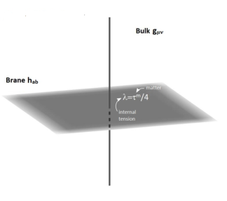
Figure 1: Consequences of the junction conditions for the braneworld models with the non-local ${R{+}RF\left(\Box\right)R}$ theory in the 5-dimensional bulk. The internal tension $\lambda$ of the 4-dimensional brane is given purely by the trace of the energy-momentum tensor of the matter confined to the brane ${\tau^{\textrm{m}}\equiv h^{ab}\tau_{ab}^{\textrm{m}}}$.

VI.2 Junction conditions in star models

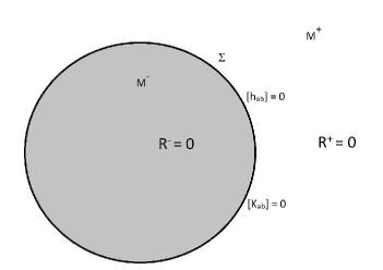
Figure 2: Consequences of the junction conditions in the non-local ${R{+}RF\left(\Box\right)R}$ theory for star models with vanishing Ricci scalar in the exterior, ${R^{+}=0}$. The infinite number of conditions implies that the Ricci scalar is zero also in the interior, ${R^{-}=0}$.

The fact that the proper junction conditions (65) impose so many constraints strongly affects the possible metrics that could potentially model physical situations by matching the geometries on the junction between $M^{+}$ and $M^{-}$. In order to illustrate this, we study two paradigmatic examples. First, we consider a generic static and spherically symmetric star whose exterior region has vanishing Ricci scalar. Then, we discuss a collapsing star with an interior region modelled by the Friedmann–Lemaitre–Robertson–Walker metric (FLRW) and the spherically symmetric static exterior with vanishing Ricci scalar. It turns out that in both cases the junction conditions hold only if the Ricci scalar is zero everywhere, as is illustrated schematically in Figure 2.

• This implies that most of the GR solutions that describe the interior of static stars or gravitational collapse are not compatible with a vanishing Ricci scalar exterior in this non-local theory.

Finally, let us stress that the main purpose of this section is to demonstrate the power of the junction conditions only, not to find new non-local solutions, since it would require solving highly complicated field equations of IDG.

VI.2.1 Static star

Let us consider a model of a static spherically symmetric star with the exterior region $M^{+}$ and the interior region ${M^{-}}$ separated by a timelike hypersurface $\Sigma$. The geometry on both sides is described by the metrics (see, e.g., hawking_ellis_1973 )

$$\bm{g}^{\pm}=-p^{\pm}(r)\bm{\mathrm{d}}t^{2}+q^{\pm}(r)\bm{\mathrm{d}}r^{2}+r^{2}\left(\bm{\mathrm{d}}\vartheta^{2}+\sin^{2}\vartheta\,\bm{\mathrm{d}}\varphi^{2}\right)\;,$$ (71)

where ${p^{\pm}(r)>0}$ and ${q^{\pm}(r)>0}$ are four single-variable functions. The junction hypersurface $\Sigma$ is located at ${r=r_{0}}$. It is clear that one indispensable condition from the continuity of the metric is

$$p^{-}(r_{0})=p^{+}(r_{0})\;,\quad q^{-}(r_{0})=q^{+}(r_{0})\;.$$ (72)

Since we are interested in the situation without any matter concentrated on $\Sigma$, we have to ensure that the proper matching conditions (65) are satisfied (${\mathcal{T}_{\mu\nu}=0}$).

First we focus on the vanishing jump of the extrinsic curvature. The induced metric on $\Sigma$, which coincides from both sides, reads

$$\bm{h}^{-}=\bm{h}^{+}=-p^{\pm}(r_{0})\bm{\mathrm{d}}t^{2}+r_{0}^{2}(\bm{\mathrm{d}}\vartheta^{2}+\sin^{2}\vartheta\,\bm{\mathrm{d}}\varphi^{2})\;.$$ (73)

Defining the orthonormal 1-forms, which are orthogonal to $\Sigma$ and pointed towards $M^{+}$,

$$\bm{n}^{-}=\bm{n}^{+}=\sqrt{q^{\pm}(r_{0})}\,\bm{\mathrm{d}}r\;,$$ (74)

we obtain the extrinsic curvature from both side of the hypersurface ${r=r_{0}}$,

$$\bm{K}^{\pm}=\frac{-p^{\pm}{}^{\prime}(r_{0})}{2\sqrt{q^{\pm}(r_{0})}}\bm{\mathrm{d}}t^{2}+\frac{r_{0}}{\sqrt{q^{\pm}(r_{0})}}\bm{\mathrm{d}}\vartheta^{2}+\frac{r_{0}\sin^{2}\vartheta}{\sqrt{q^{\pm}(r_{0})}}\bm{\mathrm{d}}\varphi^{2}\;.$$ (75)

The condition ${[\bm{K}]=0}$ together with the continuity of $q$ demands also the continuity of $p^{\prime}$,

$$p^{-}{}^{\prime}(r_{0})=p^{+}{}^{\prime}(r_{0})\;.$$ (76)

Let us move on to the junction conditions involving the Ricci scalar $R$. A significant progress can be made if we suppose that the Ricci scalar is identically zero in the exterior region $M^{+}$,

$$R^{+}=0\;.$$ (77)

Under this assumption, the junction conditions for the jump of the Ricci scalar and its derivatives can be rewritten as

$$\left.\Box^{k}R^{-}\right|_{r=r_{0}}=0\;,\quad\left.\partial_{r}\Box^{k}R^{-}\right|_{r=r_{0}}=0\;,\quad k\geq 0\;,$$ (78)

where we used the fact that the Ricci scalar as well as its derivatives depend only on the coordinate $r$. Suppressing ${\pm}$ signs, we write the explicit expression for the action of the wave operator associated with the interior metric on an arbitrary $r$-dependent scalar field ${\phi(r)}$,

$$\Box\phi(r)=\alpha\left(r\right)\phi^{\prime}(r)+\beta\left(r\right)\phi^{\prime\prime}(r)\;,$$ (79)

where we denoted

$$\alpha\left(r\right)\equiv\frac{1}{2q(r)^{2}}\left[\left(\frac{p^{\prime}(r)}{p(r)}+\frac{4}{r}\right)q(r)-q^{\prime}(r)\right]\;,\quad\beta\left(r\right)\equiv\frac{1}{q(r)}\;.$$ (80)

Employing (79), we obtain the recursive formula for $\Box^{k}R$,

$$\Box^{k}R=\alpha\left(r\right)\partial_{r}\Box^{k-1}R+\beta\left(r\right)\partial_{r}^{2}\Box^{k-1}R\;.$$ (81)

The last expression allows us to rewrite the junction conditions (78) purely in terms of partial derivatives with respect to $r$. The reasoning goes as follows: At ${k=0}$, the Ricci scalar and its first derivative must be zero at ${r=r_{0}}$. At ${k=1}$, the first condition of (78) is just a sum of first and second derivatives. Since ${\beta^{-}(r_{0})\neq 0}$ (from continuity of $q$ at $r_{0}$), the second derivative must also vanish. Going to the second condition of (78) for ${k=1}$, which is a sum of first, second, and third derivatives, we find that the third derivative is zero as well thanks to ${\beta^{-}(r_{0})\neq 0}$. Extending this iterative argument to any $k\geq 0$, it is now clear that the conditions (78) can be re-expressed as

$$\left.\partial_{r}^{k}R^{-}\right|_{r=r_{0}}=0\;,\quad k\geq 0\;.$$ (82)

Therefore, by assuming analyticity of $R$, we find that ${R}$ vanishes throughout the whole manifold $M$. This gives an explicit equation for $f$ and $g$ that is valid in everywhere in ${M^{-}}$ as well as in ${M^{+}}$,

$$R=\frac{r^{2}qp^{\prime 2}+rp\left(rp^{\prime}q^{\prime}-2q\left(rp^{\prime\prime}+2p^{\prime}\right)\right)+4p^{2}\left(rq^{\prime}+q^{2}-q\right)}{2r^{2}p^{2}q^{2}}=0\;.$$ (83)

This equation (83) and its derivatives enable us to express the $k$-th derivative of functions $p^{-}$ at ${r=r_{0}}$ as

$$\partial_{r}^{k}p^{-}(r_{0})=\Phi_{k}\big{(}p^{-}(r_{0}),p^{-}{}^{\prime}(r_{0}),q^{-}(r_{0}),q^{-}{}^{\prime}(r_{0}),\dots,\partial_{r}^{k-1}q^{-}(r_{0})\big{)}\;,$$ (84)

where we formally eliminated the dependence on $\partial_{r}^{l}p^{-}(r_{0})$, ${2\leq l\leq k-1}$, by successive substitutions. The freedom in the choice of $\partial_{r}^{k}q^{-}(r_{0})$ for ${k\geq 1}$ can be translated to the statement that all the junction conditions are satisfied for an arbitrary function $q^{-}(r)$ and a function $p^{-}(r)$ that is calculated from equation (83).

It is important to stress that all these properties follow purely from the junction conditions. Since the theory is now well-defined in the theory of distributions, we can move on to the field equations. Usually this is an extremely difficult task, but our situation is greatly simplified thanks to the condition (83). Indeed, the field equations of the theory (39) reduce everywhere just to

$$R_{\mu\nu}=T_{\mu\nu}\;,$$ (85)

which is effectively equivalent to the Einstein field equations with vanishing scalar curvature. For this reason, such solutions with ${R=0}$ everywhere (if they are regular) are the same as the GR solutions, and thus they are independent of the length scale of non-locality $\mathcal{\ell}$.

Since we are interested in star models with the vacuum outside ${r>r_{0}}$, we put ${T_{\mu\nu}^{+}=0}$. This is only solved by the Schwarzschild spacetime,

$$p^{+}(r)=1-\frac{2m}{r}\;,\quad q^{+}(r)=\bigg{(}1-\frac{2m}{r}\bigg{)}^{\!\!-1}\;,$$ (86)

where $m$ is a positive constant corresponding to mass of the star. The only possible matter allowed in the interior region ${r<r_{0}}$ (if any regular solution exists) is then given by a traceless energy-momentum tensor ${T^{-}_{\mu\nu}}$, i.e., ${T^{-}=0}$. As a consequence, the matter inside the star cannot be modelled by common perfect fluids as it usual in GR bernui1994study . For example, the well-known Tolman stars Tolman:1934za with the Schwarzschild exterior are not solutions of IDG. Thus, if we want to describe the interior of a spherically symmetric and static star with a non-traceless energy-momentum tensor, ${T^{-}\neq 0}$, then the exterior geometry cannot have vanishing Ricci scalar ${R^{+}}$.

VI.2.2 Collapsing star

In this section we shall consider a model of a collapsing star where the interior is described by a closed FLRW metric (positive spatial curvature) in co-moving coordinates,

$$\bm{g}^{-}=-\bm{\mathrm{d}}\tau^{2}+a^{2}\left(\tau\right)\left(\bm{\mathrm{d}}\lambda^{2}+\sin^{2}\lambda\,(\bm{\mathrm{d}}\vartheta^{2}+\sin^{2}\vartheta\,\bm{\mathrm{d}}\varphi^{2})\right)\;,$$ (87)

where $a\left(\tau\right)$ is the scale factor. The junction surface is located at ${\lambda=\lambda_{0}}$. The 4-velocity of the observer co-moving with the surface is ${\bm{u}=\bm{\partial}_{\tau}}$, see poisson2004relativist . The exterior is given by the spherically symmetric static geometry (with ${p^{+}>0}$ and ${q^{+}>0}$),

$$\bm{g}^{+} =-p^{+}(r)\bm{\mathrm{d}}t^{2}+q^{+}(r)\bm{\mathrm{d}}r^{2}+r^{2}\left(\bm{\mathrm{d}}\vartheta^{2}+\sin^{2}\vartheta\,\bm{\mathrm{d}}\varphi^{2}\right)\;,$$ (88)

$$=-\big{(}p^{+}(r)\dot{t}^{2}-q^{+}(r)\dot{r}^{2}\big{)}\bm{\mathrm{d}}\tau^{2}+\big{(}{-}p^{+}(r)t^{\prime}{}^{2}+q^{+}(r)r^{\prime}{}^{2}\big{)}\bm{\mathrm{d}}\lambda^{2}+r^{2}\left(\bm{\mathrm{d}}\vartheta^{2}+\sin^{2}\vartheta\,\bm{\mathrm{d}}\varphi^{2}\right)\;,$$

where we performed a generic transformation ${t=t(\tau,\lambda)}$, ${r=r(\tau,\lambda)}$ in the second line (and hid the explicit dependence on $\tau$ and $\lambda$). We use the shortcuts ${\dot{f}\equiv\partial_{\tau}f}$ and ${f^{\prime}\equiv\partial_{\lambda}f}$.

First we focus on the restrictions coming from that the continuity of the metric and the continuity of the extrinsic curvature. From the inside the induce metric reads

$$\bm{h}^{-}=-\bm{\mathrm{d}}\tau^{2}+a^{2}\left(\tau\right)\sin^{2}\lambda_{0}\,(\bm{\mathrm{d}}\vartheta^{2}+\sin^{2}\vartheta\,\bm{\mathrm{d}}\varphi^{2})\;,$$ (89)

while from the outside it can be expressed as

$$\bm{h}^{+}=-\Big{(}p^{+}\big{(}r(\tau,\lambda_{0})\big{)}\dot{t}^{2}(\tau,\lambda_{0})-q^{+}\big{(}r(\tau,\lambda_{0})\big{)}\dot{r}^{2}(\tau,\lambda_{0})\Big{)}\bm{\mathrm{d}}\tau^{2}+r^{2}(\tau,\lambda_{0})\left(\bm{\mathrm{d}}\vartheta^{2}+\sin^{2}\vartheta\,\bm{\mathrm{d}}\varphi^{2}\right)\;.$$ (90)

By comparing (89) with (90), it becomes clear that the continuity of ${\bm{h}}$ implies

$$r\left(\tau,\lambda_{0}\right)=a\left(\tau\right)\sin\lambda_{0}\;,\quad\dot{t}(\tau,\lambda_{0})p^{+}(\tau,\lambda_{0})=\sqrt{p^{+}(\tau,\lambda_{0})(1+q^{+}(\tau,\lambda_{0})\dot{r}^{2}(\tau,\lambda_{0}))}\equiv\Psi(\tau)\;.$$ (91)

The second expression can be used to obtain $t(\tau,\lambda_{0})$ by direct integration

$$t(\tau,\lambda_{0})=\int^{\tau}\!\!d\tilde{\tau}\,\frac{\Psi(\tilde{\tau})}{p^{+}(\tilde{\tau},\lambda_{0})}\;.$$ (92)

Following the arguments in Section II.2, we can now argue that also $\bm{g}$ is continuous. Consider the orthonormal 1-form orthogonal to ${\lambda=\lambda_{0}}$ and directed towards $M^{+}$. We immediately see that from the interior it reads

$$\bm{n}^{-}=a\left(\tau\right)\bm{\mathrm{d}}\lambda\;.$$ (93)

Realizing that orthonormal 1-form (pointed towards ${M^{+}}$) is actually defined uniquely by the conditions ${\bm{n}\cdot\bm{e}_{(a)}=0}$ and ${\bm{n}\cdot\bm{n}^{\sharp}=1}$ with $\bm{e}_{(a)}$ being the vector frame tangent to the hypersurface ${\lambda=\lambda_{0}}$ (e.g., ${\bm{e}_{(0)}\equiv\bm{u}}$, ${\bm{e}_{(1)}\equiv r^{-1}\bm{\partial}_{\vartheta}}$, ${\bm{e}_{(2)}\equiv(r\sin\vartheta)^{-1}\bm{\partial}_{\varphi}}$), we arrive at

$$\bm{n}^{+}=\bm{n}^{-}=-\dot{r}(\tau,\lambda_{0})\,\bm{\mathrm{d}}t+\dot{t}(\tau,\lambda_{0})\,\bm{\mathrm{d}}r\;.$$ (94)

As a results, the metric $\bm{g}$ is continuous due to ${\bm{g}=\bm{h}+\bm{n}\bm{n}}$. Having defined the orthonormal 1-form, we can now calculate and compare the extrinsic curvatures from both sides of the hypersurface. For the interior side one gets

$$\bm{K}^{-}=a\left(\tau\right)\cos\lambda_{0}\sin\lambda_{0}\,(\bm{\mathrm{d}}\vartheta^{2}+\sin^{2}\vartheta\bm{\mathrm{d}}\varphi^{2})\;,$$ (95)

and for the exterior

$$\bm{K}^{+}=\bigg{(}{-}\frac{\dot{\Psi}}{\dot{r}}\bm{\mathrm{d}}\tau^{2}+a\left(\tau\right)\Psi(\tau)\sin\lambda_{0}\,(\bm{\mathrm{d}}\vartheta^{2}+\sin^{2}\vartheta\bm{\mathrm{d}}\varphi^{2})\bigg{)}\;.$$ (96)

By demanding that the jump of the extrinsic curvature is zero, ${\bm{K}}$, we find that $\Psi(\tau)$ is constant,

$$\Psi(\tau)=\cos\lambda_{0}\;.$$ (97)

Hence, from the continuity of the metric and the extrinsic curvature have obtained the following relations

$$r\left(\tau,\lambda_{0}\right)=a\left(\tau\right)\sin\lambda_{0}\;,\quad t(\tau,\lambda_{0})=\cos\lambda_{0}\int^{\tau}\!\!\,\frac{d\tilde{\tau}}{p^{+}(\tilde{\tau},\lambda_{0})}\;.$$ (98)

Let us now focus on the remaining junction conditions, which put restrictions on the jump of the Ricci scalar. Assuming that the exterior geometry has vanishing Ricci scalar, ${R^{+}=0}$, we can write in co-moving coordinates

$$\Box^{k}R^{-}\big{|}_{\lambda=\lambda_{0}}=0\;,\qquad\partial_{\tau}\Box^{k}R^{-}\big{|}_{\lambda=\lambda_{0}}=0\;,\qquad k\geq 0\;.$$ (99)

The Ricci scalar of the interior closed FLRW metric is given by

$$R^{-}=\frac{6}{a^{2}}\left(1+\dot{a}^{2}+a\ddot{a}\right)\;.$$ (100)

Since the repeated action of the wave operator reads

$$\Box^{k}R^{-}=-3\frac{\dot{a}\left(\tau\right)}{a\left(\tau\right)}\partial_{\tau}\Box^{k-1}R^{-}-\partial_{\tau}^{2}\Box^{k-1}R^{-}\;,$$ (101)

We can make a very similar argument to the one we did for the static case. Following these steps, one can find that the conditions (99) can be rewritten as

$$\partial_{\tau}^{k}R^{-}\big{|}_{\lambda=\lambda_{0}}=0\;,\qquad k\geq 0\;.$$ (102)

Again, assuming the analyticity of $R$, this clearly implies that the Ricci scalar must be zero not only in the exterior but also throughout the whole interior region. The equation ${R^{-}=0}$ has the following solution

$$a\left(\tau\right)=\sqrt{(\tau_{*}-\tau_{0})^{2}-(\tau-\tau_{0})^{2}}\;,$$ (103)

where $\tau_{*}$ and $\tau_{0}$ are arbitrary constants. As before, we can see that the non-local character of the theory causes that the constraints themselves affect the whole spacetime and determine the geometry to a great extent. In particular, they imply that the Ricci scalar must vanish everywhere, ${R=0}$. Thus, even without solving the field equations we already see that the our simple model with the closed FLRW interior and spherically symmetric static exterior of vanishing Ricci scalar (e.g., the Schwarzschild metric) does not allow bounce. A more complicated geometry in the exterior is required.

Finally let us comment on the interior geometry with (103). The scale-factor ${a(\tau)}$ has the maximum value at ${\tau=\tau_{0}}$ and decreases towards ${\tau=\tau_{*}}$, which corresponds to the curvature singularity as can be seen from the Kretschmann scalar,

$$R_{\mu\nu\kappa\lambda}R^{\mu\nu\kappa\lambda}=\frac{24(\tau_{*}-\tau_{0})^{4}}{(\tau-\tau_{*})^{4}(\tau-2\tau_{0}+\tau_{*})^{4}}\;.$$ (104)

Unfortunately, due to the singular behaviour the check whether this geometry is a regular solution is highly non-trivial and goes beyond the scope of this paper. Our statement that ${R=0}$ is only valid outside the point of singularity ${\tau<\tau_{*}}$. In order to check that a singular geometry is a solution of IDG one should first include the singular point to the manifold as well and describe the Ricci scalar using non-linear generalized functions localized at ${\tau=\tau_{*}}$. As a next step one could calculate the action of $F(\Box)$ on $R$, for instance, using the decomposition into the eigenfunctions of $\Box$. Such a study is very challenging and has never been done even for the simplest cases such as the Schwarzschild metric.

VII Conclusions

In this paper we found the junction conditions, junction field equations for the non-local infinite derivative theory ${R+RF(\Box)R}$ (IDG). To achieve that, we relied on the theory of linear distributions to describe the potential discontinuities and we assumed that the conditions can be imposed by avoiding ill-defined expressions term by term in the infinite sums (ignoring their regularizing and deregularizing properties). After introducing necessary tools of distributional theory and the infinite derivative gravity, we obtained the matching conditions (48) by requiring that the theory is well-behaved in a distributional sense, These conditions are much more restrictive than in the general relativity (GR) or other local theories of gravity. They say that the trace of the extrinsic curvature as well as ${\Box^{k}R}$ and ${\bm{\nabla}\Box^{k}R}$ for all ${k\geq 0}$ must be continuous across the matching hypersurface.

The junction field equations and the allowed matter content on the hypersurface get also modified in IDG, see (62) with (55). Similar to GR, the external flux and external tension are not present (which is not the case of ${R+R^{2}}$, for example), but unlike in GR the energy-momentum on the hypersurface must be traceless. From there it also follows that the proper matching with no matter on the hypersurface requires vanishing jump of the extrinsic curvature.

Finally, we illustrated the use of our results in several physically motivated scenarios. First, we focused on the implications for the braneworld models with 5-dimensional bulk theory being IDG. It turns out that the internal tension of the brane is then given purely by the trace of the energy-momentum tensor of the matter confined to the brane. Next, we studied the consequences of the junction conditions on two simple examples of static and collapsing stars. In particular, we found that having a spherically symmetric static exterior with zero Ricci scalar implies that the Ricci scalar in the interior region must either be non-analytic or also vanish. These examples demonstrate that the junction condition of non-local theories hugely constraint the possible metrics that one can consider even before going into the field equations. Of course, much more difficult task is to check whether the resulting geometry actually is a solution or not. To answer this question, new methods of solving non-local nonlinear equations in curved geometry must be developed.

To conclude, let us point out that this work can be extended by considering terms of the form $R_{\mu\nu}F_{2}(\Box)R^{\mu\nu}$ and $R_{\mu\nu\kappa\lambda}F_{3}(\Box)R^{\mu\nu\kappa\lambda}$ in the action. This will of course impose more constraints on the jumps of the curvature, possibly reaching a point where only completely smooth metrics with no matter content on the hypersurface will be allowed. An even more interesting problem is the study that goes beyond our simplifying assumptions especially the case where the non-local operator can produce a singular part when it acts on a smooth function. We plan to investigate these extensions in our future works.

References

- (1) C. W. Misner, K. Thorne and J. Wheeler, Gravitation. W. H. Freeman, San Francisco, 1973.
- (2) K. Lanczos, Flächenhafte verteilung der materie in der einsteinschen gravitationstheorie, Annalen der Physik 379 (1924) 518–540, [https://onlinelibrary.wiley.com/doi/pdf/10.1002/andp.19243791403].
- (3) G. Darmois, Les équations de la gravitation einsteinienne. Gauthier-Villars Paris, 1927.
- (4) A. Lichnerowicz, Théories relativistes de la gravitation et de l’électromagnétisme: relativité générale et théories unitaires. Masson, Paris, 1955.
- (5) S. O’Brien and J. L. Synge, Jump conditions at discontinuities in general relativity, Commun. Dublin Inst. Adv. Stud., A (1952) .
- (6) L. Bel and A. Hamoui, Les conditions de raccordement en relativité générale, in Annales de l’IHP Physique théorique, vol. 7, pp. 229–244, 1967.
- (7) A. Taub, Spacetimes with distribution valued curvature tensors, Journal of Mathematical Physics 21 (1980) 1423–1431.
- (8) W. Bonnor and P. Vickers, Junction conditions in general relativity, General Relativity and Gravitation 13 (1981) 29–36.
- (9) C. Clarke and T. Dray, Junction conditions for null hypersurfaces, Classical and Quantum Gravity 4 (1987) 265.
- (10) C. Barrabes, Singular hypersurfaces in general relativity: a unified description, Classical and Quantum Gravity 6 (1989) 581.
- (11) M. Mars and J. M. Senovilla, Geometry of general hypersurfaces in space-time: Junction conditions, Class. Quant. Grav. 10 (1993) 1865–1897, [gr-qc/0201054].
- (12) W. Israel, Singular hypersurfaces and thin shells in general relativity, Nuovo Cim. B 44S10 (1966) 1.
- (13) C. Barrabes and W. Israel, Thin shells in general relativity and cosmology: The lightlike limit, Physical Review D 43 (1991) 1129.
- (14) S. C. Davis, Generalized Israel junction conditions for a Gauss-Bonnet brane world, Phys. Rev. D 67 (2003) 024030, [hep-th/0208205].
- (15) R. A. Battye and B. Carter, Generic junction conditions in brane world scenarios, Phys. Lett. B 509 (2001) 331–336, [hep-th/0101061].
- (16) N. Deruelle, M. Sasaki and Y. Sendouda, Junction conditions in f(R) theories of gravity, Prog. Theor. Phys. 119 (2008) 237–251, [0711.1150].
- (17) T. Clifton, P. Dunsby, R. Goswami and A. M. Nzioki, On the absence of the usual weak-field limit, and the impossibility of embedding some known solutions for isolated masses in cosmologies with f(R) dark energy, Phys. Rev. D 87 (2013) 063517, [1210.0730].
- (18) J. M. Senovilla, Junction conditions for F(R)-gravity and their consequences, Phys. Rev. D 88 (2013) 064015, [1303.1408].
- (19) G. J. Olmo and D. Rubiera-Garcia, Junction conditions in Palatini gravity, Class. Quant. Grav. 37 (2020) 215002, [2007.04065].
- (20) S. Vignolo, R. Cianci and S. Carloni, On the junction conditions in -gravity with torsion, Class. Quant. Grav. 35 (2018) 095014, [1801.08344].
- (21) B. Reina, J. M. M. Senovilla and R. Vera, Junction conditions in quadratic gravity: thin shells and double layers, Class. Quant. Grav. 33 (2016) 105008, [1510.05515].
- (22) W. Arkuszewski, W. Kopczynski and V. Ponomarev, Matching Conditions in the Einstein-Cartan Theory of Gravitation, Commun. Math. Phys. 45 (1975) 183–190.
- (23) A. Macias, C. Lammerzahl and L. O. Pimentel, Matching conditions in metric affine gravity, Phys. Rev. D 66 (2002) 104013.
- (24) A. Padilla and V. Sivanesan, Boundary Terms and Junction Conditions for Generalized Scalar-Tensor Theories, JHEP 08 (2012) 122, [1206.1258].
- (25) A. de la Cruz-Dombriz, P. K. S. Dunsby and D. Saez-Gomez, Junction conditions in extended Teleparallel gravities, JCAP 12 (2014) 048, [1406.2334].
- (26) T. Biswas, A. Mazumdar and W. Siegel, Bouncing universes in string-inspired gravity, JCAP 03 (2006) 009, [hep-th/0508194].
- (27) T. Biswas, E. Gerwick, T. Koivisto and A. Mazumdar, Towards singularity and ghost free theories of gravity, Phys. Rev. Lett. 108 (2012) 031101, [1110.5249].
- (28) T. Biswas, A. S. Koshelev and A. Mazumdar, Gravitational theories with stable (anti-)de Sitter backgrounds, Fundam. Theor. Phys. 183 (2016) 97–114, [1602.08475].
- (29) T. Biswas, T. Koivisto and A. Mazumdar, Towards a resolution of the cosmological singularity in non-local higher derivative theories of gravity, JCAP 11 (2010) 008, [1005.0590].
- (30) E. Tomboulis, Superrenormalizable gauge and gravitational theories, arXiv preprint hep-th/9702146 (1997) .
- (31) L. Modesto, Super-renormalizable Quantum Gravity, Phys. Rev. D 86 (2012) 044005, [1107.2403].
- (32) S. Talaganis, T. Biswas and A. Mazumdar, Towards understanding the ultraviolet behavior of quantum loops in infinite-derivative theories of gravity, Class. Quant. Grav. 32 (2015) 215017, [1412.3467].
- (33) S. Abel and N. A. Dondi, UV Completion on the Worldline, JHEP 07 (2019) 090, [1905.04258].
- (34) S. Abel, L. Buoninfante and A. Mazumdar, Nonlocal gravity with worldline inversion symmetry, JHEP 01 (2020) 003, [1911.06697].
- (35) S. Abel and D. Lewis, Worldline theories with towers of internal states, JHEP 12 (2020) 069, [2007.07242].
- (36) G. Calcagni, L. Modesto and G. Nardelli, Initial conditions and degrees of freedom of non-local gravity, JHEP 05 (2018) 087, [1803.00561].
- (37) I. Kolar and A. Mazumdar, Hamiltonian for scalar field model of infinite derivative gravity, Phys. Rev. D 101 (2020) 124028, [2003.00590].
- (38) L. Buoninfante, G. Harmsen, S. Maheshwari and A. Mazumdar, Nonsingular metric for an electrically charged point-source in ghost-free infinite derivative gravity, Phys. Rev. D 98 (2018) 084009, [1804.09624].
- (39) J. Boos, V. P. Frolov and A. Zelnikov, Gravitational field of static p -branes in linearized ghost-free gravity, Phys. Rev. D 97 (2018) 084021, [1802.09573].
- (40) J. Boos, J. Pinedo Soto and V. P. Frolov, Ultrarelativistic spinning objects in nonlocal ghost-free gravity, Phys. Rev. D 101 (2020) 124065, [2004.07420].
- (41) I. Kolář and A. Mazumdar, NUT charge in linearized infinite derivative gravity, Phys. Rev. D 101 (2020) 124005, [2004.07613].
- (42) L. Buoninfante, A. S. Cornell, G. Harmsen, A. S. Koshelev, G. Lambiase, J. a. Marto et al., Towards nonsingular rotating compact object in ghost-free infinite derivative gravity, Phys. Rev. D 98 (2018) 084041, [1807.08896].
- (43) V. P. Frolov and A. Zelnikov, Head-on collision of ultrarelativistic particles in ghost-free theories of gravity, Phys. Rev. D 93 (2016) 064048, [1509.03336].
- (44) V. P. Frolov, A. Zelnikov and T. de Paula Netto, Spherical collapse of small masses in the ghost-free gravity, JHEP 06 (2015) 107, [1504.00412].
- (45) V. P. Frolov, Mass-gap for black hole formation in higher derivative and ghost free gravity, Phys. Rev. Lett. 115 (2015) 051102, [1505.00492].
- (46) E. Kilicarslan, Weak Field Limit of Infinite Derivative Gravity, Phys. Rev. D 98 (2018) 064048, [1808.00266].
- (47) S. Dengiz, E. Kilicarslan, I. Kolář and A. Mazumdar, Impulsive waves in ghost free infinite derivative gravity in anti-de Sitter spacetime, Phys. Rev. D 102 (2020) 044016, [2006.07650].
- (48) A. de la Cruz-Dombriz, F. J. Maldonado Torralba and A. Mazumdar, Nonsingular and ghost-free infinite derivative gravity with torsion, Phys. Rev. D 99 (2019) 104021, [1812.04037].
- (49) Á. de la Cruz-Dombriz, F. J. M. Torralba and A. Mazumdar, Ghost-free higher-order theories of gravity with torsion, arXiv preprint arXiv:1911.08846 (2019) .
- (50) L. Schwartz, Sur l’impossibilité de la multiplication des distributions, C. R. Acad. Sci. Paris 239 (1954) 847–8.
- (51) J. F. Colombeau, Multiplication of distributions, Bull. Amer. Math. Soc. (N.S.) 23 (10, 1990) 251–268.
- (52) R. Steinbauer and J. A. Vickers, The Use of generalised functions and distributions in general relativity, Class. Quant. Grav. 23 (2006) R91–R114, [gr-qc/0603078].
- (53) M. Grosser, M. Kunzinger, M. Oberguggenberger and R. Steinbauer, Geometric theory of generalized functions with applications to general relativity. Mathematics and Its Applications. Springer, Dordrecht, 2001, 10.1007/978-94-015-9845-3.
- (54) T. Biswas, A. Conroy, A. S. Koshelev and A. Mazumdar, Generalized ghost-free quadratic curvature gravity, Class. Quant. Grav. 31 (2014) 015022, [1308.2319].
- (55) J. M. Senovilla, Gravitational double layers, Class. Quant. Grav. 31 (2014) 072002, [1402.1139].
- (56) R. Maartens and K. Koyama, Brane-World Gravity, Living Rev. Rel. 13 (2010) 5, [1004.3962].
- (57) E. Flanagan, N. T. Jones, H. Stoica, S. Tye and I. Wasserman, A Brane world perspective on the cosmological constant and the hierarchy problems, Phys. Rev. D 64 (2001) 045007, [hep-th/0012129].
- (58) L. Randall and R. Sundrum, A Large mass hierarchy from a small extra dimension, Phys. Rev. Lett. 83 (1999) 3370–3373, [hep-ph/9905221].
- (59) L. Randall and R. Sundrum, An Alternative to compactification, Phys. Rev. Lett. 83 (1999) 4690–4693, [hep-th/9906064].
- (60) T. Shiromizu, K.-i. Maeda and M. Sasaki, The Einstein equation on the 3-brane world, Phys. Rev. D 62 (2000) 024012, [gr-qc/9910076].
- (61) S. Forste, Fine tuning of the cosmological constant in brane worlds, Fortsch. Phys. 49 (2001) 495–501, [hep-th/0012029].
- (62) S. W. Hawking and G. F. R. Ellis, The Large Scale Structure of Space-Time. Cambridge Monographs on Mathematical Physics. Cambridge University Press, 1973, 10.1017/CBO9780511524646.
- (63) A. Bernui and E. Portocarrero, Study of the matching of solutions of the Einstein equations according to Darmois, The Astrophysical Journal 427 (1994) 947–950.
- (64) R. C. Tolman, Effect of imhomogeneity on cosmological models, Proc. Nat. Acad. Sci. 20 (1934) 169–176.
- (65) E. Poisson, A relativist’s toolkit: the mathematics of black-hole mechanics. Cambridge university press, 2004.
- (66) J. Heinzle and R. Steinbauer, Remarks on the distributional Schwarzschild geometry, J. Math. Phys. 43 (2002) 1493–1508, [gr-qc/0112047].