Abstract

We theoretically investigate the self-evaporation dynamics of quantum droplets in a ⁴¹K-⁸⁷Rb mixture, in free-space. The dynamical formation of the droplet and the effects related to the presence of three-body losses are analyzed by means of numerical simulations. We identify a regime of parameters allowing for the observation of the droplet self-evaporation in a feasible experimental setup.

1 1 0 Received: date; Accepted: date; Published: date Self-evaporation dynamics of quantum droplets in a ⁴¹K-⁸⁷Rb mixture Chiara Fort ^1,2 and Michele Modugno ^3,4* Chiara Fort and Michele Modugno Correspondence: michele.modugno@ehu.eus

1 Introduction

As demonstrated in a seminal paper by D. Petrov Petrov (2015), ultracold quantum gases can exist in the form of self-bound droplets that do not expand even in the absence of any confinement. This liquid-like behavior, which originates from the interplay of attractive mean-field interactions and the repulsive effect of quantum fluctuations Petrov (2018); Ferrier-Barbut and Pfau (2018); Ferrier-Barbut (2019), was successfully observed in a number of experiments with dipolar condensates Ferrier-Barbut et al. (2016a, b); Schmitt et al. (2016); Chomaz et al. (2016); Tanzi et al. (2019), homonuclear mixtures of ³⁹K Cabrera et al. (2018); Semeghini et al. (2018); Cheiney et al. (2018); Ferioli et al. (2018), and recently in a heteronuclear mixture of ⁴¹K and ⁸⁷Rb D’Errico et al. (2019); Burchianti et al. (2020). These findings have triggered an intense research activity on droplets properties (see, e.g., the recent reviews in Refs. Böttcher et al. (2020); Luo et al. (2020)) and on the so-called Lee-Huang-Yang fluid Jørgensen et al. (2018); Minardi et al. (2019); Skov et al. (2020), and have motivated further studies in low-dimensional systems Morera et al. (2020); Lavoine and Bourdel (2020) and also beyond Petrov’s theory Hu et al. (2020); Hu and Liu (2020a, b); Zin et al. (2020); Ota and Astrakharchik (2020).

Besides being self bound, one of the most peculiar characteristics of these quantum objects is the fact that they can be self-evaporating. Namely, in certain regimes the droplet cannot sustain any collective mode, such that any initial excitation is completely dissipated (that is, evaporated) until the system relaxes into a droplet with a lower number of atoms. This remarkable feature, originally predicted in Ref. Petrov (2015) for bosonic mixtures, has been so far elusive to the experimental detection. Indeed, the first pioneering experiments performed with bosonic mixtures Cabrera et al. (2018); Semeghini et al. (2018) have shown that the homonuclear mixtures of ³⁹K suffer from strong three-body losses that continuously drive the system out of equilibrium, and eventually lead to the depletion of the droplet. This behavior was then confirmed by the theoretical analysis reported in Ref. Ferioli et al. (2019), where the complex dynamics taking place during the droplet formation is thoroughly described. There, it was shown that the evolution of the system is indeed dominated by the presence of three-body losses and by a continuous release of atoms to restore the proper population ratio, whereas the self-evaporation mechanism plays only a negligible role, if any.

In this respect, the recent experiment in Ref. D’Errico et al. (2019) represents a promising setup in which the self-evaporation mechanism could be properly investigated. As a matter of fact, for a ⁴¹K-⁸⁷Rb mixture the regime of parameters for which self-bound droplets form is such that three-body losses are expected to be significantly suppressed. Indeed, in such a mixture droplets form at lower densities $n\sim(\delta g/g)^{2}a^{-3}$, and this allows for a larger ratio $\tau_{\mathrm{life}}/\tau\sim n^{-1}$, with $\tau_{\mathrm{life}}$ and $\tau$ being respectively the lifetime (limited by three-body losses) and the characteristic time scale of the droplet dynamics D’Errico et al. (2019). Thus, the fact that the ⁴¹K-⁸⁷Rb mixture is characterized by larger scattering lengths with respect to the ³⁹K mixture employed in Refs. Cabrera et al. (2018); Semeghini et al. (2018) allows for lower densities and, therefore, longer lifetimes. Actually, in that experiment no appreciable effect of three-body losses was observed on the timescale of several tens of milliseconds.

Motivated by the previous discussion, in this paper we analyze the self-evaporation mechanism and the role of three-body losses on the collective excitations of a ⁴¹K-⁸⁷Rb quantum droplet. For the sake of conceptual clarity, and in view of the fact that quantum droplets at equilibrium are spherically symmetric objects, we shall restrict the analysis to the case of a spherically symmetric system. Though this assumption limits the study to the monopole collective mode, it is however sufficient to draw the general behavior of the system and to discuss the role of three-body losses.

The paper is organized as follows. In Section 2 we review the general formalism for describing quantum droplets in heteronuclear bosonic mixtures. Then, in Section 3 we discuss the preparation of the initial state, namely a droplet compressed by a harmonic trapping. The dynamics of the droplet after the release of the trap is then studied in Section 4 in the unitary case (no losses), and in the presence of three-body losses. Finally, in Section 5 we draw the conclusions.

2 Self-bound droplets

We consider a binary condensate of ⁴¹K and ⁸⁷Rb atoms in the $\left|F=1,m_{F}=1\right\rangle$ state, as considered in the recent experiment in Ref. D’Errico et al. (2019). The two components will be indicated as 1 and 2, respectively. This system is described by the following Gross-Pitaevskii (GP) energy functional, including both the mean field term and the Lee-Huang-Yang (LHY) correction accounting for quantum fluctuations in the local density approximation: Ancilotto et al. (2018)

$$E=\sum_{i=1}^{2}\int\left[\frac{\hbar^{2}}{2m_{i}}|\nabla\psi_{i}(\bm{r})|^{2}+V_{i}(\bm{r})n_{i}(\bm{r})\right]d\bm{r}+\frac{1}{2}\sum_{i,j=1}^{2}g_{ij}\int n_{i}(\bm{r})n_{j}(\bm{r})d\bm{r}+\int{\cal E}_{\rm LHY}(n_{1}(\bm{r}),n_{2}(\bm{r}))d\bm{r}\,,$$ (1)

where $m_{i}$ are the atomic masses, $V_{i}(\bm{r})$ the external potentials, and $n_{i}(\bm{r})=|\psi_{i}(\bm{r})|^{2}$ the densities of the two components ($i=1,2$). The LHY correction reads Petrov (2015)

$${\cal E}_{\rm LHY} =\frac{8}{15\pi^{2}}\left(\frac{m_{1}}{\hbar^{2}}\right)^{3/2}\!\!\!\!\!\!(g_{11}n_{1})^{5/2}f\left(\frac{m_{2}}{m_{1}},\frac{g_{12}^{2}}{g_{11}g_{22}},\frac{g_{22}\,n_{2}}{g_{11}\,n_{1}}\right)$$

$$\equiv\kappa(g_{11}n_{1})^{5/2}f(z,u,x),$$ (2)

with $\kappa=8m_{1}^{3/2}/(15\pi^{2}\hbar^{3})$ and $f(z,u,x)>0$ being a dimensionless function of the parameters $z\equiv m_{2}/m_{1}$, $u\equiv g_{12}^{2}/(g_{11}g_{22})$, and $x\equiv g_{22}n_{2}/(g_{11}n_{1})$ Petrov (2015); Ancilotto et al. (2018). The mixture is completely characterized in terms of the intraspecies $g_{ii}=4\pi\hbar^{2}a_{i}/m_{i}$ ($i=1,2$), and interspecies $g_{12}=2\pi\hbar^{2}a_{12}/m_{12}$ coupling constants, where $m_{12}=m_{1}m_{2}/(m_{1}+m_{2})$ is the reduced mass. The values of the homonuclear scattering lengths are fixed to $a_{11}=62a_{0}$ , $a_{22}=100.4a_{0}$, whereas the heteronuclear scattering length $a_{12}$ is considered here as a free parameter, that can be tuned by means of Feshbach resonances D’Errico et al. (2019). The onset of the MF collapse regime corresponds to $\delta g=g_{12}+\sqrt{g_{1}g_{2}}=0$, at $a_{\mathrm{12}}^{c}=-73.6a_{0}$ Riboli and Modugno (2002).

In free space ($V_{i}\equiv 0$), the equilibrium density of a droplet is obtained by requiring the vanishing of the total pressure Astrakharchik and Malomed (2018), which yields Petrov (2015)

$$n^{0}_{1} =\frac{25\pi}{1024}\frac{1}{a_{11}^{3}}\frac{\delta g^{2}}{g_{11}g_{22}}f^{-2}\left(\frac{m_{2}}{m_{1}},1,\sqrt{\frac{g_{22}}{g_{11}}}\right)$$ (3)

$$n^{0}_{2} =n^{0}_{1}\sqrt{\frac{g_{11}}{g_{22}}}.$$ (4)

Following Petrov (2015); Ancilotto et al. (2018), we consider this function at the mean-field collapse $u=1$, $f(z,1,x)$. We note that the actual expression for $f$ can be fitted very accurately with the same functional form of the homonuclear case Minardi et al. (2019)

$$f\left(\frac{m_{2}}{m_{1}},1,\sqrt{\frac{g_{22}}{g_{11}}}\right)\simeq\left[1+\left(\frac{m_{2}}{m_{1}}\right)^{3/5}\!\!\!\!\sqrt{\frac{g_{22}}{g_{11}}}\right]^{5/2}.$$ (5)

For a finite number of atoms the droplet has a finite size, and it can be effectively described by a single wave function that satisfies the following dimensionless equation Petrov (2015)

$$\left[-\frac{1}{2}\nabla_{\tilde{\bm{r}}}^{2}-3\widetilde{N}|\phi_{0}|^{2}+\frac{5}{2}\widetilde{N}^{3/2}|\phi_{0}|^{3}\right]\phi_{0}=\tilde{\mu}\phi_{0},$$ (6)

with $\int|\phi_{0}|^{2}d\tilde{\bm{r}}=1$, and

$$N_{i}=n_{i}^{(0)}\xi^{3}\widetilde{N},$$ (7)

where $\sum_{i}N_{i}=N$ and $N_{1}/N_{2}=\sqrt{g_{22}/g_{11}}$ [see Eq. (4)]. Here $\xi$ represents the length scale of the droplet Petrov (2015); Hu and Liu (2020b)

$$\xi =\hbar\left[\frac{3}{2}\frac{\sqrt{g_{11}}/m_{2}+\sqrt{g_{22}}/m_{1}}{|\delta g|\sqrt{g_{11}}n_{1}^{(0)}}\right]^{1/2},$$ (8)

and $n_{i}^{(0)}$ the equilibrium density of each component in the uniform case. We also remind that the wave functions of the two condensates forming the droplet are given by $\psi_{i}=\sqrt{n_{i}^{(0)}}\phi_{0}$.

3 Preparation of the initial state

Following Ref. D’Errico et al. (2019), we initially prepare the atomic mixture in the ground state of an optical dipole trap. In order to simplify the discussion, and motivated by the fact that quantum droplets at equilibrium are spherically symmetric objects, we assume i) that the two condensates are initially prepared in a spherically symmetric potential $U^{d}_{j}(r)$ ($j=1,2$), and ii) that the differential vertical gravitational sag (due to the different masses of the two atomic species) can be exactly compensated. With these assumptions, which will be maintained throughout this work for easiness of calculations and conceptual clarity, both the ground state and the dynamical evolution can be obtained by solving spherically symmetric equations. We remark that this approach restricts the analysis to the excitations of the monopole mode only. Indeed, the excitation of surface modes (with angular momentum $\ell\neq 0$), which arise when the condensate is prepared in an asymmetric trap, is ruled out by the assumption of spherical symmetry. However, the presence of these modes is not expected to modify qualitatively the picture resulting from the following discussion.

The ground state of the system is obtained by minimizing the energy functional in Eq. (1) by means of a steepest-descent algorithm Press et al. (2007). Formally, this corresponds to solve the following set of stationary Gross-Pitaevskii (GP) equations for two wave functions $\psi_{j}$ Dalfovo et al. (1999)

$$\left[-\frac{\hbar^{2}}{2m_{1}}\nabla^{2}_{r}+U^{d}_{1}(r)+\mu_{1}(n_{1},n_{2})\right]\psi_{1}=\mu_{1}\psi_{1}$$

(9)

$$\left[-\frac{\hbar^{2}}{2m_{2}}\nabla^{2}_{r}+U^{d}_{2}(r)+\mu_{2}(n_{1},n_{2})\right]\psi_{2}=\mu_{2}\psi_{2},$$

where $\nabla_{r}^{2}$ represents the radial component of the Laplacian:

$$\nabla_{r}^{2}={\frac{1}{r^{2}}}{\frac{\partial}{\partial r}}\left(r^{2}{\frac{\partial}{\partial r}}\right)={\frac{\partial^{2}}{\partial r^{2}}}+{\frac{2}{r}}{\frac{\partial}{\partial r}}.$$ (10)

The local chemical potentials $\mu_{i}(n_{1},n_{2})$ include both the usual mean-field term and the Lee-Huang-Yang (LHY) correction Petrov (2015), namely

$$\mu_{i}(n_{1},n_{2})=g_{ii}n_{i}+g_{12}n_{j}+\frac{\delta E_{LHY}}{\delta n_{i}},\quad i\neq j,$$ (11)

with $n_{i}(r)\equiv|\psi_{i}(r)|^{2}$.

We recall that the optical dipole potential experienced by the two atomic species can be written as $U^{d}_{j}(r)=U_{0j}I(r)$, where $U_{0j}$ is species-dependent ($j=1,2$) and it depends on the atomic species polarizability and the wavelength of the optical potential, and $I(r)$ represents the intensity of the laser beam. For the atomic mixture ⁴¹K-⁸⁷Rb and a wavelength $\lambda=1064$ nm D’Errico et al. (2019) one has $\alpha\equiv U_{02}/U_{01}\simeq 1.15$. Then, in the harmonic approximation, we have

$$U^{d}_{j}(r)=\frac{1}{2}m_{j}\omega^{2}_{j}r^{2},$$ (12)

with $\omega_{1}=\omega_{2}\sqrt{m_{2}/(\alpha m_{1})}$. In the following, the value of the trap frequency will be considered as a free parameter, to be tuned in order to produce the desired amount of initial excitations. For low enough $\omega_{j}$, the droplet will be prepared close to the equilibrium configuration in free space, whereas a tight confinement obviously corresponds to the excitation of a compressional mode.

The other free parameters of the system are the inter-species scattering length $a_{12}$, that we will consider in the range $a_{12}\in[-95,-73.6]a_{0}$, below to the mean-field collapse threshold, and the number of atoms of the two species. As for the latter, we shall vary $N_{2}$ in the range $[1.5,15]\times 10^{4}$, keeping $N_{1}=N_{2}\sqrt{g_{22}/g_{11}}$, so that the atom numbers match the nominal equilibrium ratio in Eq. (4).

4 Dynamics

Once the initial state is prepared, the optical dipole trap is switched off and the system is let to evolve. The droplet dynamics is studied here by solving the following set of GP equations Wächtler and Santos (2016a, b); Ferioli et al. (2019)

$$i\hbar\partial_{t}\psi_{1}=\left[-\frac{\hbar^{2}\nabla^{2}_{r}}{2m_{1}}+\mu_{1}(n_{1},n_{2})-i\hbar\frac{K_{3}}{2}|\psi_{2}|^{4}\right]\psi_{1}$$

(13)

$$i\hbar\partial_{t}\psi_{2}=\left[-\frac{\hbar^{2}\nabla^{2}_{r}}{2m_{2}}+\mu_{2}(n_{1},n_{2})-i\hbar K_{3}|\psi_{1}|^{2}|\psi_{2}|^{2}\right]\psi_{2},$$

in the presence of three-body losses, which are included by adding to the energy functional in Eq. (1) a dissipative term $-(i/2)\hbar K_{3}\int n_{1}(\bm{r},t)n_{2}(\bm{r},t)^{2}d^{3}r$ (with $K_{3}=7\times 10^{-41}$ m⁶/s, see Ref. D’Errico et al. (2019)) accounting for the dominant recombination channel, i.e. K-Rb-Rb.

Since the droplet is prepared in a compressed configuration (owing to the presence of the trap), the droplet will start oscillating. According to discussion in Ref. Petrov (2015), in the absence of three-body losses the dynamics is expected to be characterized either by sinusoidal oscillations of the droplet width, where the monopole mode exists, or by damped oscillations, in the so-called self-evaporation regime. The latter represents one of the remarkable properties of quantum droplets Petrov (2015); Ferioli et al. (2019), and it takes place in a certain window of $\widetilde{N}$, where the excitation spectrum of the droplet lies entirely in the continuum. The nominal phase diagram for our system (obtained from the predictions Ref. Petrov (2015)) is shown in Fig. 1 as a function of the interspecies scattering length $a_{12}$ and of the (initial) number of atoms $N_{2}$. The specific combination of parameters used in the figure, $(\widetilde{N}-N_{c})^{1/4}$, is introduced after Ref. Petrov (2015). The monopole mode is expected to be stable for $\widetilde{N}>933.7$, and to evaporate for lower values of $\widetilde{N}$. In the window $94.2<\widetilde{N}<933.7$ other modes with $\ell\neq 0$ (not included in the present discussion) may appear, whereas below $\widetilde{N}<94.2$ neither the monopole nor the surface modes ($\ell\neq 0$) can be sustained, such that the droplet is expected to evaporate any initial excitation Petrov (2015). Below $\widetilde{N}_{c}$, where a droplet cannot be formed, the mixture forms a so-called LHY fluid: in this regime the MF interactions almost cancel out ($\delta g/\sqrt{g_{11}g_{22}}\approx 0$), and the system is governed only by quantum fluctuations Jørgensen et al. (2018); Minardi et al. (2019); Skov et al. (2020).

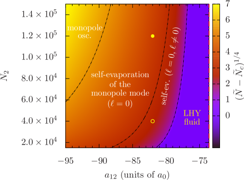
Figure 1: Heat map of $(\widetilde{N}-\widetilde{N}_{c})^{1/4}$ as a function of $a_{12}$ and $N_{2}$, with $\widetilde{N}_{c}=18.65$ being the critical value for the existence of a droplet Petrov (2015). The dotted-dashed lines, corresponding to $\widetilde{N}=933.7$, $94.2$, $18.65$ (from left to right), represent the boundaries between the different regimes (see text). The vertical red dashed-dotted line at $a_{12}=-73.6$ corresponds to the onset of the MF collapse. The two circles at $a_{12}=-82a_{0}$ refer to the parameter configurations considered in Sec. 4.

4.1 Estimate of the droplet lifetime

Before analyzing the detailed dynamical behavior of our system it is convenient to discuss the role of three-body losses on the droplet lifetime. To this aim, we shall consider a droplet in free space, at equilibrium (at $t=0$). Then, assuming that the shape of the droplet is weakly affected by the atom losses (which is justified at the early stages at the evolution, at least), we can write

$$n_{i}(r,t)\simeq N_{i}(t)\rho(r),$$ (14)

where $N_{1}(0)/N_{2}(0)=\sqrt{g_{22}/g_{11}}\equiv\gamma$ , and with $\rho(r)$ representing the droplet density profile normalized to unity [see Eqs. (4) and (7)]. With this in mind, the evolution of $N_{i}(t)$ can be obtained from the previous Eqs. (13) by neglecting the kinetic and chemical potential terms [which concur in determining the shape $\rho(r)$], left multiplying each equation by $\psi_{i}^{*}$, and integrating over the volume (see also Ref. Altin et al. (2011)), yielding

$$\frac{d\bar{N}_{1}}{d\tau}=-\bar{N}_{1}\bar{N}_{2}^{2}$$ (15)

$$\frac{d\bar{N}_{2}}{d\tau}=-2\gamma\bar{N}_{1}\bar{N}_{2}^{2},$$ (16)

where we have defined $\bar{N}_{i}(\tau)\equiv N_{i}(\tau)/N_{i}(0)$ and $\tau\equiv tK_{3}N_{2}^{2}(0)\int\rho^{3}d^{3}r$. Notice that the factor of $2$ in Eq. (16) corresponds to the fact that here we are considering the dominant recombination channel K-Rb-Rb (two atoms of Rb are lost for each atom of K).

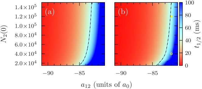
Figure 2: Heat map of $t_{1/2}$ as a function of $a_{12}$ and $N_{2}(0)$. (a) Prediction of the analytical model, see Eq. (18); (b) values extracted from the actual decay of $N_{2}(t)$ obtained from the solution of the GP equations in (13). The color scale is saturated at $t_{1/2}=100$ ms (dark blue). The dashed-dotted line corresponds to $t_{1/2}=50$ ms. The two circles at $a_{12}=-82a_{0}$ refer to the parameter configurations considered in the GP simulations of Sec. 4.2.

The above equations have an approximate solution of the form

$$\bar{N}_{1}(\tau) =\frac{1-\beta}{1+(\tau/\tau_{1})^{\alpha_{1}}}+\beta,$$ (17)

$$\bar{N}_{2}(\tau) =\frac{1}{1+(\tau/\tau_{2})^{\alpha_{2}}},$$ (18)

which is very accurate, indeed. In the present case ($\gamma\simeq 0.8736$), from a fit of the exact numerical solution of Eqs. (15) and (16) we find $\tau_{1}\simeq 0.70$, $\alpha_{1}\simeq 0.88$, $\beta\simeq 0.43$, $\tau_{2}\simeq 0.71$, $\alpha_{2}\simeq 0.86$. In particular, $\tau_{2}$ corresponds to the half-life of the $i=2$ component (regardless of the value of $\alpha_{2}$), in which losses are dominant. Therefore, it represents a characteristic time through which we can measure the impact of three-body losses on the lifetime of the droplet. In our simple model the half-life is therefore $t_{1/2}\simeq\tau_{2}/\left[K_{3}N_{2}^{2}(0)\int\rho^{3}d^{3}r\right]$ that, besides the explicit dependence on $N_{2}(0)$, also depends implicitly on $a_{12}$ through the density distribution $\rho(r)$. The behavior of $t_{1/2}$ as a function of $a_{12}$ and $N_{2}(0)$ is shown in Fig. 2. There we compare the prediction of the above analytical model with the actual values obtained from the solution of the GP equations in (13). The qualitative agreement is remarkable.

4.2 Damped monopole oscillations

Given the above picture, in the following we shall investigate the self evaporation dynamics for $a_{12}=-82a_{0}$, where the droplet half-life is larger than $50$ ms [see Fig. 2(b)]. In particular, we consider two different configurations with $N_{2}=4\times 10^{4}$ and $N_{2}=1.2\times 10^{5}$, indicated by the yellow circles in Figs. 1 and 2(b), both lying in the self-evaporation regime. It is worth to remark that in the regime where the monopole mode is expected to be stable (see Fig. 1) the droplet is affected by severe three-body losses (see Fig. 2), which make the detection of this mode unfeasible.

In order to distinguish between the atoms remaining in the droplet and those that evaporate, we define the droplet volume as that contained within a certain bulk radius. In the present case, it can be conveniently fixed to $R_{d}=8$ $\mu$m . Accordingly, with $N_{i}^{d}(t)$ we indicate the number of atoms of each species ($i=1,2$) within the droplet volume, at time $t$. Then, we define a running value of $\widetilde{N}$ as Ferioli et al. (2019)

$$\widetilde{N}_{R}(t)\equiv\frac{1}{\xi^{3}}\frac{N_{1}^{d}(t)+N_{2}^{d}(t)}{N_{1}+N_{2}}=k\sum_{i=1}^{2}N_{i}^{d}(t),$$ (19)

where $k\simeq 4.41\times 10^{-3}$ for the current values of the scattering lengths.

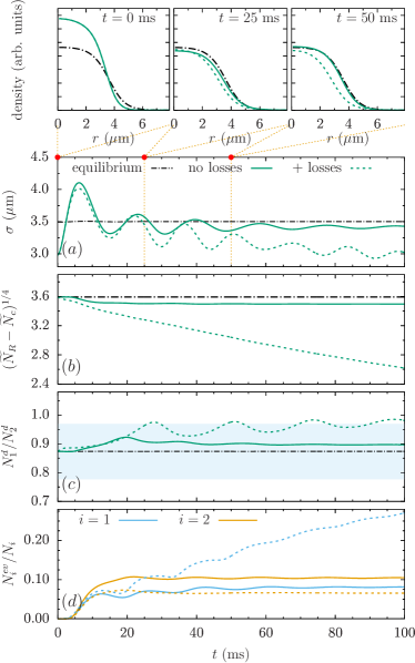
Figure 3: Evolution of (a) the droplet width $\sigma(t)$, (b) the running value of $\widetilde{N}_{R}(t)$ (see text), (c) the ratio $N_{1}^{d}(t)/N_{2}^{d}(t)$, and (d) the fraction of evaporated atoms for each species $N_{i}^{ev}(t)/N_{i}$, after the release from a trap of frequency $\omega_{2}=2\pi\times 50$ Hz, with and without three-body losses. The insets in the top row show the total density of the binary mixture, $n(r,t)=\sum_{i=1}^{2}N_{i}|\psi_{i}(r,t)|^{2}$, at different evolution times, corresponding to the red circles in (a). The horizontal line in (b) represent the nominal equilibrium value $N_{1}/N_{2}=\sqrt{g_{22}/g_{11}}\simeq 0.873$, and the dashed area the corresponding tolerance (see text). Here $a_{12}=-82a_{0}$, $N_{2}=4\times 10^{4}$ (left), $N_{2}=1.5\times 10^{5}$ (right).

The evolution of the system is shown in in Fig. 3, where we plot the rms width $\sigma(t)$ of the droplet, the running value of $[\widetilde{N}_{R}(t)-N_{c}]^{1/4}$, the ratio $N_{1}^{d}(t)/N_{2}^{d}(t)$, and the fraction of evaporated atoms for each species $N_{i}^{ev}(t)/N_{i}$, with and without three-body losses. In both cases the mixture is initially prepared in the ground state of a dipole trap of frequency $\omega_{2}=2\pi\times 50$ Hz (we recall that $\omega_{1}=\omega_{2}\sqrt{m_{2}/(\alpha m_{1})}$, see Sec. 3; in the present case $\omega_{1}=2\pi\times 67.9$ Hz).

Let us first focus on the clean case, in the absence of three-body losses. As expected, we find that in both the investigated cases the droplet width performs damped sinusoidal oscillations (corresponding to a damped monopole mode), and the system eventually relaxes to an equilibrium configuration [see Fig. 3(a), along with the top panels], corresponding to a smaller, stationary value of $\widetilde{N}_{R}(t)$, see panels (b). This decrease in the number of particles is a consequence of the self-evaporation mechanism Petrov (2015); Ferioli et al. (2019), which takes place within the first $15$ ms. Looking at panel (d), where we plot the fraction of atoms of each species that are lost by self-evaporation, it is clear that the values of $N_{i}^{ev}(t)/N_{i}$ soon reach their asymptotic value (modulo small fluctuations). In addition, also the ratio between the atom numbers in the two components remains close to the equilibrium value, see panels (c), with deviations below the reequilibration threshold (shaded area in the figure). Indeed, we recall that a droplet can sustain an excess of particles in one of the two components $\delta N_{i}^{d}/N_{i}^{d}$ up to a critical value $\sim\delta g/\sqrt{g_{11}g_{22}}$ Petrov (2015) ($\approx 11\%$ in the present case), beyond which particles in excess are expelled.

Let us now discus how the presence of three-body losses affects the above picture. From panels (b) it is evident that losses produce a continuous drain of particles from the droplet. Nevertheless, after $100$ ms of evolution the value of $\widetilde{N}_{R}(t)$ is still well above the critical value $\widetilde{N}_{c}$ for the existence of a droplet. Indeed, after several tens of milliseconds the mixture still forms a self-bound droplet (see e.g. the density profile at $50$ ms) which keeps undergoing damped monopole oscillations, as shown in panels (a). Notably, the initial stage of the evolution is still dominated by self-evaporation, see panel (d), and then both the frequency and the amplitude of the oscillations become larger than in the clean case (without losses), because of the atoms that leave the bulk and populate the tails. Actually, there are two opposite effects taking place: on the one hand the droplet shrinks because of the loss of atoms due to three-body recombination, on the other hand there is an outward flow of K atoms that evaporate from the droplet, see panel (d). This species selective evaporation is due to the fact that the major loss of atoms affects the Rb component (see previous section), so that a progressively increasing fraction of K atoms cannot stay bound inside the droplet, and it is let free to expand. We remark that this is obviously a non-equilibrium process, as it is evident from the fact that $\widetilde{N}_{R}(t)$ does not relaxes to a stationary value and that the ratio $N_{1}^{d}(t)/N_{2}^{d}(t)$ soon run over the reequilibration threshold, anyway. All this is responsible for the different ’asymptotic’ behavior of $\sigma(t)$ in the two cases shown in panels (a). For $N_{2}=4\times 10^{4}$ (left), the two effects approximately compensate each other, and the width oscillates close to the nominal equilibrium value without losses. Instead, for $N_{2}=1.5\times 10^{5}$ (right), which is characterized by a shorter lifetime, the droplet width decreases progressively (though keeping oscillating). It is worth to remark that the actual behavior is also sensitive to the choice of the droplet radius $R_{d}$.

5 Conclusions

We have theoretically investigated the self-evaporation dynamics of quantum droplets in a ⁴¹K-⁸⁷Rb mixture in feasible experimental setups, including the effects of three-body losses. The mixture is prepared in the ground state of a spherically symmetric harmonic trap, that is then released thus letting the system evolve in free space. The subsequent dynamics, characterized by the excitation of the monopole breathing mode, has been analyzed by solving the coupled Gross-Pitaevskii equations for the two components. For the estimated values of three-body losses ($K_{3}=7\times 10^{-41}$ m⁶/s for the dominant recombination channel K-Rb-Rb D’Errico et al. (2019)), we find that by tuning the interspecies scattering length $a_{12}$, the lifetime of the system can be easily adjusted to be of the order of, or larger than, $100$ ms. This makes ⁴¹K-⁸⁷Rb droplets much more robust than those realized with two hyperfine states of ³⁹K, whose lifetime is limited to the order of $10$ ms Cabrera et al. (2018); Semeghini et al. (2018); Ferioli et al. (2019). Such long lifetimes permits to follow the droplet dynamics for several tens of milliseconds, without any appreciable loss of resolution. In this scenario, we have found that the initial stage of the evolution is dominated by the self-evaporation mechanism even in the presence of three-body losses, and that the latter induce an interesting non equilibrium dynamics at later times. These findings make the experimental investigation of collective modes of self-bound droplets in ⁴¹K-⁸⁷Rb mixtures very promising.

This work was supported by the Spanish Ministry of Science, Innovation and Universities and the European Regional Development Fund FEDER through Grant No. PGC2018-101355-B-I00 (MCIU/AEI/FEDER, UE), by the Basque Government through Grant No. IT986-16.

Appendix A Numerical methods

Let us consider a GP equation of the form

$$i\partial_{\tau}\varphi(r,\tau)=H\varphi(r,\tau),$$ (20)

with

$$H=-\frac{1}{2}\nabla_{r}^{2}+V(r)+g|\varphi(r,\tau)|^{2},$$ (21)

and

$$\nabla^{2}={\frac{\partial^{2}}{\partial r^{2}}}+\frac{2}{r}{\frac{\partial}{\partial r}}.$$ (22)

The Crank-Nicholson algorithm (on a discrete space-time grid) consists in solving the following system of linear equations with the components of the vector $\varphi^{n+1}\equiv(\varphi_{1},\dots,\varphi_{j},\dots\varphi_{N})^{n+1}$ being the unknown variables Press et al. (2007)

$$\left(1+{\frac{i\Delta\tau}{2}}H\right)\varphi^{n+1}=\left(1-{\frac{i\Delta\tau}{2}}H\right)\varphi^{n}.$$ (23)

Notice that this algorithm preserves the unitarity for real-time evolutions.

Derivatives can be written in terms of central differences Abramowitz and Stegun (1964),

$$\frac{\partial^{2}\varphi}{\partial r^{2}} \to\frac{\varphi_{j+1}-2\varphi_{j}+\varphi_{j-1}}{\Delta^{2}}$$ (24)

$$\frac{2}{r}\frac{\partial\varphi}{\partial r} \to\frac{2}{r_{j}}\frac{\varphi_{j+1}-\varphi_{j-1}}{2\Delta}$$ (25)

that allow to write the linear system Eq. (23) in the following tridiagonal form,

$$a_{j}\varphi^{n+1}_{j-1}+b_{j}\varphi^{n+1}_{j}+c_{j}\varphi^{n+1}_{j+1}=d_{j}.$$ (26)

The explicit expression for the coefficients $a_{j}$, $b_{j}$, $c_{j}$ , and $d_{j}$ ($j=1,\dots N$) are

$$a_{j} ={\frac{i\Delta\tau}{2}}\left[\frac{1}{\Delta^{2}}-\frac{1}{r_{j}\Delta}\right],$$ (27)

$$b_{j} =1+{\frac{i\Delta\tau}{2}}\left[-\frac{2}{\Delta^{2}}+V(r_{j})+g|\varphi_{j}^{n}|^{2}\right],$$ (28)

$$c_{j} ={\frac{i\Delta\tau}{2}}\left[\frac{1}{\Delta^{2}}+\frac{1}{r_{j}\Delta}\right],$$ (29)

$$d_{j} =-a_{j}\varphi^{n}_{j-1}+(2-b_{j})\varphi^{n}_{j}-c_{j}\varphi^{n}_{j+1},$$ (30)

which have to be accompanied by suitable boundary conditions in order to preserve the tridiagonal form.

References yes

References

- Petrov (2015) Petrov, D.S. Quantum Mechanical Stabilization of a Collapsing Bose-Bose Mixture. Phys. Rev. Lett. 2015, 115, 155302. doi:\changeurlcolorblack10.1103/PhysRevLett.115.155302.
- Petrov (2018) Petrov, D.S. Liquid beyond the van der Waals paradigm. Nature Physics 2018, 14, 211–212. doi:\changeurlcolorblack10.1038/s41567-018-0052-9.
- Ferrier-Barbut and Pfau (2018) Ferrier-Barbut, I.; Pfau, T. Quantum liquids get thin. Science 2018, 359, 274–275. doi:\changeurlcolorblack10.1126/science.aar3785.
- Ferrier-Barbut (2019) Ferrier-Barbut, I. Ultradilute Quantum Droplets. Physics Today 2019, 72, 46–52. doi:\changeurlcolorblack10.1063/pt.3.4184.
- Ferrier-Barbut et al. (2016a) Ferrier-Barbut, I.; Kadau, H.; Schmitt, M.; Wenzel, M.; Pfau, T. Observation of Quantum Droplets in a Strongly Dipolar Bose Gas. Phys. Rev. Lett. 2016, 116, 215301. doi:\changeurlcolorblack10.1103/PhysRevLett.116.215301.
- Ferrier-Barbut et al. (2016b) Ferrier-Barbut, I.; Schmitt, M.; Wenzel, M.; Kadau, H.; Pfau, T. Liquid quantum droplets of ultracold magnetic atoms. Journal of Physics B: Atomic, Molecular and Optical Physics 2016, 49, 214004. doi:\changeurlcolorblack10.1088/0953-4075/49/21/214004.
- Schmitt et al. (2016) Schmitt, M.; Wenzel, M.; Böttcher, F.; Ferrier-Barbut, I.; Pfau, T. Self-bound droplets of a dilute magnetic quantum liquid. Nature 2016, 539, 259 EP –.
- Chomaz et al. (2016) Chomaz, L.; Baier, S.; Petter, D.; Mark, M.J.; Wächtler, F.; Santos, L.; Ferlaino, F. Quantum-Fluctuation-Driven Crossover from a Dilute Bose-Einstein Condensate to a Macrodroplet in a Dipolar Quantum Fluid. Phys. Rev. X 2016, 6, 041039. doi:\changeurlcolorblack10.1103/PhysRevX.6.041039.
- Tanzi et al. (2019) Tanzi, L.; Lucioni, E.; Famà, F.; Catani, J.; Fioretti, A.; Gabbanini, C.; Bisset, R.N.; Santos, L.; Modugno, G. Observation of a Dipolar Quantum Gas with Metastable Supersolid Properties. Phys. Rev. Lett. 2019, 122, 130405. doi:\changeurlcolorblack10.1103/PhysRevLett.122.130405.
- Cabrera et al. (2018) Cabrera, C.R.; Tanzi, L.; Sanz, J.; Naylor, B.; Thomas, P.; Cheiney, P.; Tarruell, L. Quantum liquid droplets in a mixture of Bose-Einstein condensates. Science 2018, 359, 301–304. doi:\changeurlcolorblack10.1126/science.aao5686.
- Semeghini et al. (2018) Semeghini, G.; Ferioli, G.; Masi, L.; Mazzinghi, C.; Wolswijk, L.; Minardi, F.; Modugno, M.; Modugno, G.; Inguscio, M.; Fattori, M. Self-Bound Quantum Droplets of Atomic Mixtures in Free Space. Phys. Rev. Lett. 2018, 120, 235301. doi:\changeurlcolorblack10.1103/PhysRevLett.120.235301.
- Cheiney et al. (2018) Cheiney, P.; Cabrera, C.R.; Sanz, J.; Naylor, B.; Tanzi, L.; Tarruell, L. Bright Soliton to Quantum Droplet Transition in a Mixture of Bose-Einstein Condensates. Phys. Rev. Lett. 2018, 120, 135301. doi:\changeurlcolorblack10.1103/PhysRevLett.120.135301.
- Ferioli et al. (2018) Ferioli, G.; Semeghini, G.; Masi, L.; Giusti, G.; Modugno, G.; Inguscio, M.; Gallemì, A.; Recati, A.; Fattori, M. Collisions of self-bound quantum droplets. Physical Review Letters 2018, 122, 090401, [1812.09151]. doi:\changeurlcolorblack10.1103/physrevlett.122.090401.
- D’Errico et al. (2019) D’Errico, C.; Burchianti, A.; Prevedelli, M.; Salasnich, L.; Ancilotto, F.; Modugno, M.; Minardi, F.; Fort, C. Observation of quantum droplets in a heteronuclear bosonic mixture. Phys. Rev. Research 2019, 1, 033155. doi:\changeurlcolorblack10.1103/PhysRevResearch.1.033155.
- Burchianti et al. (2020) Burchianti, A.; D’Errico, C.; Prevedelli, M.; Salasnich, L.; Ancilotto, F.; Modugno, M.; Minardi, F.; Fort, C. A Dual-Species Bose-Einstein Condensate with Attractive Interspecies Interactions. Condensed Matter 2020, 5. doi:\changeurlcolorblack10.3390/condmat5010021.
- Böttcher et al. (2020) Böttcher, F.; Schmidt, J.N.; Hertkorn, J.; Ng, K.S.H.; Graham, S.D.; Guo, M.; Langen, T.; Pfau, T. New states of matter with fine-tuned interactions: quantum droplets and dipolar supersolids 2020. [2007.06391].
- Luo et al. (2020) Luo, Z.; Pang, W.; Liu, B.; Li, Y.; Malomed, B.A. A new form of liquid matter: quantum droplets 2020. [2009.01061].
- Jørgensen et al. (2018) Jørgensen, N.B.; Bruun, G.M.; Arlt, J.J. Dilute Fluid Governed by Quantum Fluctuations. Phys. Rev. Lett. 2018, 121, 173403. doi:\changeurlcolorblack10.1103/PhysRevLett.121.173403.
- Minardi et al. (2019) Minardi, F.; Ancilotto, F.; Burchianti, A.; D’Errico, C.; Fort, C.; Modugno, M. Effective expression of the Lee-Huang-Yang energy functional for heteronuclear mixtures. Phys. Rev. A 2019, 100, 063636. doi:\changeurlcolorblack10.1103/PhysRevA.100.063636.
- Skov et al. (2020) Skov, T.G.; Skou, M.G.; Jørgensen, N.B.; Arlt, J.J. Observation of a Lee-Huang-Yang Fluid 2020. [2011.02745].
- Morera et al. (2020) Morera, I.; Astrakharchik, G.E.; Polls, A.; Juliá-Díaz, B. Quantum droplets of bosonic mixtures in a one-dimensional optical lattice. Physical Review Research 2020, 2, 022008. doi:\changeurlcolorblack10.1103/physrevresearch.2.022008.
- Lavoine and Bourdel (2020) Lavoine, L.; Bourdel, T. 1D to 3D beyond-mean-field dimensional crossover in mixture quantum droplets, 2020, [2011.12394].
- Hu et al. (2020) Hu, H.; Wang, J.; Liu, X.J. Microscopic pairing theory of a binary Bose mixture with interspecies attractions: Bosonic BEC-BCS crossover and ultradilute low-dimensional quantum droplets. Phys. Rev. A 2020, 102, 043301. doi:\changeurlcolorblack10.1103/PhysRevA.102.043301.
- Hu and Liu (2020a) Hu, H.; Liu, X.J. Microscopic derivation of the extended Gross-Pitaevskii equation for quantum droplets in binary Bose mixtures. Phys. Rev. A 2020, 102, 043302. doi:\changeurlcolorblack10.1103/PhysRevA.102.043302.
- Hu and Liu (2020b) Hu, H.; Liu, X.J. Collective excitations of a spherical ultradilute quantum droplet. Phys. Rev. A 2020, 102, 053303. doi:\changeurlcolorblack10.1103/PhysRevA.102.053303.
- Zin et al. (2020) Zin, P.; Pylak, M.; Gajda, M. Zero-energy modes of two-component Bose-Bose droplets, 2020, [2011.05135].
- Ota and Astrakharchik (2020) Ota, M.; Astrakharchik, G. Beyond Lee-Huang-Yang description of self-bound Bose mixtures. SciPost Physics 2020, 9, 020. doi:\changeurlcolorblack10.21468/scipostphys.9.2.020.
- Ferioli et al. (2019) Ferioli, G.; Semeghini, G.; Masi, L.; Giusti, G.; Modugno, G.; Inguscio, M.; Gallemí, A.; Recati, A.; Fattori, M. Collisions of Self-Bound Quantum Droplets. Phys. Rev. Lett. 2019, 122, 090401. doi:\changeurlcolorblack10.1103/PhysRevLett.122.090401.
- Ancilotto et al. (2018) Ancilotto, F.; Barranco, M.; Guilleumas, M.; Pi, M. Self-bound ultradilute Bose mixtures within local density approximation. Phys. Rev. A 2018, 98, 053623. doi:\changeurlcolorblack10.1103/PhysRevA.98.053623.
- Riboli and Modugno (2002) Riboli, F.; Modugno, M. Topology of the ground state of two interacting Bose-Einstein condensates. Phys. Rev. A 2002, 65, 063614. doi:\changeurlcolorblack10.1103/PhysRevA.65.063614.
- Astrakharchik and Malomed (2018) Astrakharchik, G.E.; Malomed, B.A. Dynamics of one-dimensional quantum droplets. Phys. Rev. A 2018, 98, 013631. doi:\changeurlcolorblack10.1103/PhysRevA.98.013631.
- Press et al. (2007) Press, W.H.; Teukolsky, S.A.; Vetterling, W.T.; Flannery, B.P. Numerical Recipes: The Art of Scientific Computing, 3 ed.; Cambridge University Press: USA, 2007.
- Dalfovo et al. (1999) Dalfovo, F.; Giorgini, S.; Pitaevskii, L.P.; Stringari, S. Theory of Bose-Einstein condensation in trapped gases. Rev. Mod. Phys. 1999, 71, 463–512. doi:\changeurlcolorblack10.1103/RevModPhys.71.463.
- Wächtler and Santos (2016a) Wächtler, F.; Santos, L. Ground-state properties and elementary excitations of quantum droplets in dipolar Bose-Einstein condensates. Phys. Rev. A 2016, 94, 043618. doi:\changeurlcolorblack10.1103/PhysRevA.94.043618.
- Wächtler and Santos (2016b) Wächtler, F.; Santos, L. Quantum filaments in dipolar Bose-Einstein condensates. Phys. Rev. A 2016, 93, 061603. doi:\changeurlcolorblack10.1103/PhysRevA.93.061603.
- Altin et al. (2011) Altin, P.A.; Dennis, G.R.; McDonald, G.D.; Döring, D.; Debs, J.E.; Close, J.D.; Savage, C.M.; Robins, N.P. Collapse and three-body loss in a 85Rb Bose-Einstein condensate. Phys. Rev. A 2011, 84, 033632. doi:\changeurlcolorblack10.1103/PhysRevA.84.033632.
- Abramowitz and Stegun (1964) Abramowitz, M.; Stegun, I.A. Handbook of Mathematical Functions with Formulas, Graphs, and Mathematical Tables, ninth dover printing, tenth gpo printing ed.; Dover: New York City, 1964.