Local Dvoretzky-Kiefer-Wolfowitz confidence bands

Abstract

In this paper, we revisit the concentration inequalities for the supremum of the cumulative distribution function (CDF) of a real-valued continuous distribution as established by Dvoretzky, Kiefer, Wolfowitz and revisited later by Massart in two seminal papers. We focus on the concentration of the local supremum over a sub-interval, rather than on the full domain. That is, denoting $U$ the CDF of the uniform distribution over $[0,1]$ and $U_{n}$ its empirical version built from $n$ samples, we study $\mathbb{P}\Big{(}\sup_{u\in[\underline{u},\overline{u}]}U_{n}(u)-U(u)>\varepsilon\Big{)}$ for different values of $\underline{u},\overline{u}\in[0,1]$. Such local controls naturally appear for instance when studying estimation error of spectral risk-measures (such as the conditional value at risk), where $[\underline{u},\overline{u}]$ is typically $[0,\alpha]$ or $[1-\alpha,1]$ for a risk level $\alpha$, after reshaping the CDF $F$ of the considered distribution into $U$ by the general inverse transform $F^{-1}$. Extending a proof technique from Smirnov, we provide exact expressions of the local quantities $\mathbb{P}\Big{(}\sup_{u\in[\underline{u},\overline{u}]}U_{n}(u)-U(u)>\varepsilon\Big{)}$ and $\mathbb{P}\Big{(}\sup_{u\in[\underline{u},\overline{u}]}U(u)-U_{n}(u)>\varepsilon\Big{)}$ for each $n,\varepsilon,\underline{u},\overline{u}$. Interestingly these quantities, seen as a function of $\varepsilon$, can be easily inverted numerically into functions of the probability level $\delta$. Although not explicit, they can be computed and tabulated. We plot such expressions and compare them to the classical bound $\sqrt{\frac{\log(1/\delta)}{2n}}$ provided by Massart inequality. We then provide an application of such result to the control of generic functional of the CDF, motivated by the case of the conditional value at risk. Last, we extend the local concentration results holding individually for each $n$ to time-uniform concentration inequalities holding simultaneously for all $n$, revisiting a reflection inequality by James, which is of independent interest for the study of sequential decision making strategies.

Keywords: Cumulative Distribution Function; Concentration inequalities; DKW; Risk measure.

1 Introduction

Let $X$ be a real-valued random variable. The cumulative distribution function (CDF) $F$, that associates to each $x\!\in\!\mathbb{R}$ the quantity $F(x)=\mathbb{P}(X\leqslant x)$ has been at the heart of statistics since its early ages, as $F$ characterizes the law of $X$. The quantile function $Q(\delta)=\inf\{x\!\in\!\mathbb{R}:F(x)\geqslant\delta\}$ enables to simulate the random variable, since $X\stackrel{{\scriptstyle\mathcal{L}}}{{=}}Q(Y)$, where $Y$ is uniform on $[0,1]$. More generally one can reduce the study of the supremum of $F_{n}(x)-F(x)$ over a set $\mathcal{X}$, where $F_{n}$ is the empirical version of $F$ built from $n$ i.i.d. samples of a distribution with CDF $F$ to the supremum of $U_{n}(u)-U(u)$ over its image $F(\mathcal{X})$, where $U$ denotes the CDF of the uniform distribution on $[0,1]$ and $U_{n}$ denotes its empirical version built from $n$ i.i.d. samples. The CDF is at the heart of the Glivenko-Cantelli theorem – sometimes called the fundamental theorem of statistics – that states that $\mathbb{P}(\lim_{n\to\infty}\sup_{x\in\mathbb{R}}|F_{n}(x)-F(x)|=0)=1$. This result led to the definition of $P$-Glivenko-Cantelli classes of functions $\mathcal{F}$, for which $\displaystyle{\lim_{n\to\infty}\sup_{f\in\mathcal{F}}|P_{n}(f)-P(f)|\to 0}$ almost surely, where $P(f)=\mathbb{E}[f(X)]$ denotes the measure associated to the random variable $X$, and $P_{n}$ denotes the empirical measure built from $n$ i.i.d. samples. This definition had a prominent role in the development of function process theory as Glivenko-Cantelli theorem shows that the class of functions $\mathcal{F}=\{x\mapsto\mathbb{I}\{x\leqslant t\}:t\!\in\!\mathbb{R}\}$ is an example being $P$-Glivenko-Cantelli for all probability measure $P$ on $\mathbb{R}$, which opened the quest for other such classes. While Glivenko-Cantelli classes are nice, great efforts have been put on obtaining not only asymptotic results but further understand the speed of convergence of the supremum towards $0$. One important part of the literature focuses on Donsker classes where the supremum of $\sqrt{n}(F_{n}(x)-F(x))$ is studied as a random process (See Kolmogorov (1933), wrongly extended by Donsker (1952) but later corrected; we refer the interested reader to Billingsley (1968), Pollard (1984), Dudley (1999) or Shorack and Wellner (2009) for further details and overview of the field). An alternative approach to this prolific field of research is the one proposed by Dvoretzky–Kiefer–Wolfowitz in their seminal paper Dvoretzky et al. (1956) that looks at deviation inequalities of the supremum process for each $n$. The initial result from Dvoretzky et al. (1956) is based on an exact derivation from Smirnov (1944), and shows that

$$\mathbb{P}\Big{(}\sup_{u\in[0,1]}U_{n}(u)-U(u)>\varepsilon\Big{)}\leqslant Ce^{-2n\varepsilon^{2}}\,,$$

hence providing an exponentially decreasing upper bound on the deviation probability, yet for some unspecified constant $C$. In a seminal paper, Massart (1990) later showed that the result holds for the constant $C=1$ provided that $e^{-2n\varepsilon^{2}}\leqslant 1/2$, and that this constant cannot be improved. Such a result is especially interesting as it enables the practitioner to derive tight confidence bands on CDF. Indeed, it can be used to show that for any $\delta\in[0,0.5]$, with probability higher than $1-\delta$, uniformly for all $x\in\mathbb{R}$, then

$$F_{n}(x)-\varepsilon\leqslant F(x)\leqslant F_{n}(x)+\varepsilon\quad\text{ where }\varepsilon=\sqrt{\frac{\log(2/\delta)}{2n}}\,.$$

Risk-aversion estimation

One important example of application of CDF deviation inequalities is when considering spectral risk-measures, such as the Conditional Value At Risk (CVAR) that is popular in economy (See Mandelbrot (1997); Rockafellar and Uryasev (2000)). The definition of the CVaR changes from author to author, depending on conventions, such as whether it applies to a non-negative or non-positive random variable, and whether the risk corresponds to the upper or lower tail. We choose below a non-negative random variable with focus on its lower tail for this short presentation. While CVaR at risk level $\alpha\in[0,1]$ is classically defined as an optimization (see Section 4 for more details), when the CDF $F$ of the considered random variable is a continuous bijection, it takes the following convenient form

$$\texttt{CVaR}^{r}_{\alpha}(\nu) \!=\! \mathbb{E}_{\nu}\bigg{[}X\bigg{|}X\leqslant\overline{x}_{\alpha}(\nu)\bigg{]}=\frac{1}{\alpha}\mathbb{E}\Big{[}X\mathbb{I}\{X\!\leqslant\!\overline{x}_{\alpha}(\nu)\}\Big{]}=\frac{1}{\alpha}\int_{\mathbb{R}^{+}}\!\!\max(\alpha\!-\!F(x),0)dx\,.$$

where we introduced the (upper) Value at Risk $\overline{x}_{\alpha}(\nu)=\inf\{x\!\in\!\mathbb{R}:F(x)>\alpha\}$. In particular the CVaR writes as a function of the CDF in the form $\texttt{CVaR}^{r}_{\alpha}(\nu)=h^{r}\Big{(}\int_{\mathcal{X}}g^{r}\big{(}F(x)\big{)}dx\Big{)}$, where $h^{r}$ and $g^{r}$ are known monotonic functions. Further $g^{r}(\beta)=(\alpha-\beta)_{+}$ has support $[0,\alpha)$ that is a strict subset of $[0,1]$ for $\alpha<1$, and $\alpha$ is typically small (e.g. $\alpha=0.01,\alpha=0.05$). This property is actually not limited to the CVaR risk-measure (see e.g. spectral risk-measures Acerbi (2002)) and suggests to focus on controlling the local deviations of the CDF in order to later control the risk-measure. Note also that since in this case $\sup_{x\in[0,\overline{x}_{\alpha}(\nu)]}F_{n}(x)-F(x)\stackrel{{\scriptstyle\mathcal{L}}}{{=}}\sup_{u\in[0,\alpha]}U_{n}(u)-U(u)$ and $\alpha$ is given by the practitioner, controlling the local supremum for the uniform distribution ensures a control for any unknown distribution. Hence, such results are universal in a sense, which is especially interesting when the class of distributions generating the samples is unknown to the practitioner.

Outline and contribution

The purpose of this work is not to greatly extend the vast literature on function process theory, but rather to focus specifically on the local control of the CDF concentration. Namely, we ask how to revisit the initial results from Smirnov in the case when the supremum is not considered on $\mathbb{R}$ but on a sub-interval $\mathcal{X}$. Obviously the results by DKW and Massart already apply to yield confidence bands in such cases. However, making use of the existing bound to uniformly control the deviations on a set $\mathcal{X}$ that is “small” may result in unnecessary large confidence bands that may be concerning for the practitioner. In this article, extending the proof techniques from Smirnov (1944), we derive in Section 2 exact expressions for the quantities $\mathbb{P}\Big{(}\sup_{u\in[\underline{u},\overline{u}]}U_{n}(u)-U(u)>\varepsilon\Big{)}$ (see Theorem 3) and $\mathbb{P}\Big{(}\sup_{u\in[\underline{u},\overline{u}]}U(u)-U_{n}(u)>\varepsilon\Big{)}$ (see Theorem 4) for any $n\!\in\!\mathbb{N},\varepsilon>0$ and $\underline{u},\overline{u}\!\in\![0,1]$. This derivation, up to our knowledge, is (perhaps surprisingly) novel. Interestingly, these probabilities, seen as functions of $\varepsilon$ can be inverted numerically, and directly yield confidence bands on the CDF. In Section 3, we plot these functions and their inverse, which enables to highlight their non-trivial behavior and compare them to the simplified bound obtained by application of DKW and Massart bound. This also shows that deriving approximations of the exact quantities may not be necessarily required for practical usage. Although these plots reveal the strikingly good match between the simplified and exact bound when considering the full interval $[0,1]$, which is expected since the constant $C=1$ obtained by Massart cannot be improved, they also reveal the conservative nature of the simplified bounds when considering a supremum over a sub-interval of the form $[0,\alpha]$ or $[1-\alpha,1]$ for small values of $\alpha$. We believe making use of the exact bounds may thus greatly impact the practitioner interested in tight bounds. To provide greater perspective, in Section 4, we quickly detail the case of the risk-measure known as Conditional Value At Risk. In Section  5, we finally describe a generic way to turn the concentration bounds of Section 2, valid with high probability for each $n\!\in\!\mathbb{N}$, into concentration bounds that are time-uniform, that is, valid with high probability simultaneously for all $n\!\in\!\mathbb{N}$. This extension is not trivial as it seems difficult to make use of Doob’s maximal inequality in this context, hence we describe an alternative way to derive such results that is of independent interest.

Contents

1. 1 Introduction
2. 2 Local CDF concentration
3. 3 Numerical illustration of the bounds
4. 4 Application to the CVAR and other functionals of the CDF
5. 5 Time-uniform concentration inequalities
6. A Proofs of the main results
7. B Monte Carlo simulations of the confidence bounds
8. C Technical details regarding the CVAR
9. D Other result

2 Local CDF concentration

For a distribution $\nu$ with CDF $F$, we denote by $F_{n}$ the empirical CDF built from a sample of size $n$ from $\nu$. We consider distributions with continuous CDF in the sequel. Since the uniform distribution on $[0,1]$ plays a special role, we denote its CDF by $U$ and empirical CDF with a sample of size $n$ by $U_{n}$.

Let us first recall the result obtained by Massart’s version of DKW inequality from Massart (1990).

$$\forall\delta_{0}\!\in\![0,0.5)\quad\mathbb{P}\bigg{(}\sup_{x\in\mathcal{X}}F(x)-F_{n}(x)>\sqrt{\frac{\log(1/\delta_{0})}{2n}}\bigg{)}\leqslant\delta_{0}\,.$$

$$\forall\delta_{0}\!\in\![0,0.5)\quad\mathbb{P}\bigg{(}\sup_{x\in\mathcal{X}}F_{n}(x)-F(x)>\sqrt{\frac{\log(1/\delta_{0})}{2n}}\bigg{)}\leqslant\delta_{0}\,.$$

We now introduce the following closely related quantities on which we shall focus

$$\delta_{[\underline{u},\overline{u}]}(n,\varepsilon) = \mathbb{P}\Big{(}\sup_{u\in[\underline{u},\overline{u}]}U_{n}(u)-U(u)>\varepsilon\Big{)}\quad\varepsilon_{[\underline{u},\overline{u}]}(n,\delta)=\inf\{\varepsilon:\delta_{[\underline{u},\overline{u}]}(n,\varepsilon)\leqslant\delta\}$$

$$\tilde{\delta}_{[\underline{u},\overline{u}]}(n,\varepsilon) = \mathbb{P}\Big{(}\sup_{u\in[\underline{u},\overline{u}]}U(u)-U_{n}(u)>\varepsilon\Big{)}\quad\tilde{\varepsilon}_{[\underline{u},\overline{u}]}(n,\delta)=\inf\{\varepsilon:\tilde{\delta}_{[\underline{u},\overline{u}]}(n,\varepsilon)\leqslant\delta\}\,.$$

Since in general, $U_{n}(u)\!\neq\!-U_{n}(1-u)$, then $\delta_{[\underline{u},\overline{u}]}(n,\varepsilon)$ is in general different from $\tilde{\delta}_{[\underline{u},\overline{u}]}(n,\varepsilon)$. Also, since $U_{n}-U$ is right continuous with a left limit, but $U-U_{n}$ is left continuous with a right limit, the supremum of these functions have different behavior. In particular, the following result, whose proof is immediate given this observation, shows that considering the second supremum should be considered with care.

Lemma 1 (Asymmetry)

On the one hand, the value of the optimization problem $\sup_{u\in[\alpha,\beta]}U_{n}(u)-U(u)$ is achieved at one of the points $v=u_{(k)}$ or at $v=\alpha$, where $(u_{(k)})_{k\in[n]}$ are the order samples received from the uniform distribution, such that $0\leqslant u_{(1)}\leqslant\dots\leqslant u_{(n)}\leqslant 1$.

$$\sup_{u\in[\alpha,\beta]}U_{n}(u)-U(u)=\max\bigg{\{}U_{n}(v)-U(v):v\in\{\alpha\}\cup\{u_{(1)},\dots,u_{(n)}\}\cap[\alpha,\beta]\bigg{\}}\,.$$

On the other hand, the value of the optimization problem $\sup_{u\in[\alpha,\beta]}U(u)-U_{n}(u)$ is not realized at any point, but can be approached from below when approaching some of the $v=u_{(k)}$ or point $v=\beta$ from below.

$$\sup_{u\in[\alpha,\beta]}U(u)-U_{n}(u)=\max\bigg{\{}\lim_{u\to v,u<v}U(u)-U_{n}(u):v\in\{\beta\}\cup\{u_{(1)},\dots,u_{(n)}\}\cap(\alpha,\beta]\bigg{\}}$$

To complement this lemma, let us recall that $\sup_{u\in[\alpha,\beta]}U_{n}(u)-U(u)$ and $\sup_{u\in[1-\beta,1-\alpha]}U(u)-U_{n}(u)$ should have the same law. Nevertheless, we now provide the following result that gives a first explicit expression of $\delta_{[\underline{u},\overline{u}]}$ and $\tilde{\delta}_{[\underline{u},\overline{u}]}$. For the second quantity, we make use of a construction inspired from Skorokhod convergence since the considered function is not corlol (continuous on the right with a limit on the left).

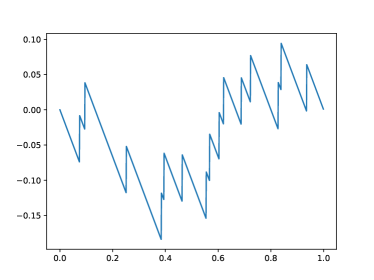
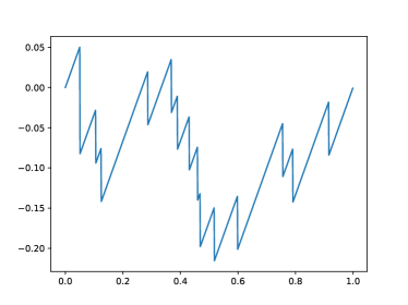
Figure 1: Illustration of the random function $u\mapsto U_{n}(u)-u$ (left) and $u\mapsto u-U_{n}(u)$ (right) using $n=15$.

Lemma 2 (Exact CDF concentration)

Let $U$ denote the CDF of a random variable uniformly distributed on $[0,1]$ (that is, $U(x)=x$). Let $U_{n}$ denote the empirical CDF built from $n$ i.i.d. samples from this distribution. Let us introduce the following notation $I_{k}(x;a_{1},\dots,a_{k})=\int_{a_{1}}^{x}\int_{a_{2}}^{t_{1}}\dots\int_{a_{k}}^{t_{k-1}}dt_{1}\dots dt_{k}$ for all $k\in\mathbb{N}_{\star}$ and $x\geqslant a_{1}\geqslant\dots\geqslant a_{k}\in\mathbb{R}$, and $I_{0}(x;\emptyset)=1$. Let $\alpha,\beta$ be such that $[\alpha,\beta]\subset[0,1]$, $\varepsilon>0$ and $n\in\mathbb{N}$. Then it holds

$$\mathbb{P}\Big{(}\sup_{u\in[\alpha,\beta]}U_{n}(u)-U(u)>\varepsilon\Big{)} = \sum_{\ell=0}^{\overline{n}_{\alpha,\varepsilon}-1}\binom{n}{\ell}\beta_{\ell+1,\varepsilon}^{n-\ell}\ell!I_{\ell}(1;\beta_{1,\varepsilon},\dots\beta_{\ell,\varepsilon})\,,$$

$$\mathbb{P}\Big{(}\sup_{u\in[\alpha,\beta]}U(u)-U_{n}(u)>\varepsilon\Big{)} = \sum_{\ell=0}^{\overline{n}_{\beta,\varepsilon}-1}\binom{n}{\ell}\tilde{\alpha}_{\ell+1,\varepsilon}^{n-\ell}\ell!I_{\ell}(1;\tilde{\alpha}_{1,\varepsilon},\dots\tilde{\alpha}_{\ell,\varepsilon})\,.$$

where we introduced $\beta_{k,\varepsilon}=\min(\beta,(n-k+1)/n-\varepsilon)$, $\tilde{\beta}=1-\beta$, $\tilde{\alpha}_{k,\varepsilon}=\min(1-\alpha,1-\varepsilon-(k-1)/n)$ as well as $\overline{n}_{\alpha,\varepsilon}=\lceil n(1-\alpha-\varepsilon)\rceil$ and $\overline{n}_{\beta,\varepsilon}=\lceil n(\beta-\varepsilon)\rceil$.

Sketch of proof of Lemma 2

We provide below a sketch of proof of the key steps leading to the control of $\sup_{u\in[\alpha,\beta]}U_{n}(u)-U(u)$ in Lemma 2. The full proof is detailed in and deferred to Appendix A. This enables to highlight the main ingredients of the proof, and in particular the smart use of a generic Taylor expansion by Smirnov, that we reuse in order to prove this novel result.

The first step of the proof consists in showing that

$$\mathbb{P}\Big{(}\sup_{u\in[\alpha,\beta]}U_{n}(u)-U(u)\leqslant\varepsilon\Big{)}$$

$$= n!\int\dots\int\mathbb{I}\bigg{\{}0\leqslant u_{1}\leqslant\dots u_{n}\leqslant 1;\forall k\in[n],\begin{cases}\text{if }u_{k}\in[\alpha,\beta]&\text{ then }u_{k}\geqslant\frac{k}{n}-\varepsilon\\ \text{if }k>n(\varepsilon+\alpha)&\text{ then }\alpha\notin[u_{k},u_{k+1})\\ \end{cases}\bigg{\}}du_{1}\dots du_{n}.$$

The second step enables to simplify the expression, leading, after careful rewriting, to

$$\mathbb{P}\Big{(}\sup_{u\in[\alpha,\beta]}U_{n}(u)-U(u)\leqslant\varepsilon\Big{)} = n!\int_{\beta_{1}}^{1}\!\int_{\beta_{2}}^{t_{1}}\!\dots\!\int_{\beta_{\overline{n}_{\alpha,\varepsilon}}}^{t_{\overline{n}_{\alpha,\varepsilon}-1}}\!\!J_{n-\overline{n}_{\alpha,\varepsilon}}(t_{\overline{n}_{\alpha,\varepsilon}})dt_{\overline{n}_{\alpha,\varepsilon}}\!\dots\!dt_{1}\!\,,$$

where $J_{k}(x)=\frac{x^{k}}{k!}$, $\beta_{k}=\min(\beta,(n-k+1)/n-\varepsilon)$ and $\overline{n}_{\alpha,\varepsilon}=\lceil n(1-\varepsilon-\alpha)\rceil$.

At this point, the key trick, originating from Smirnov (1944), is to make use of the following variant of the Taylor expansion at multiple points $a_{1},a_{2},\dots$, of the value of a smooth function $f$ at point $x$, given by

$$f(x) = f(a_{1})+\sum_{\ell=1}^{n-k-1}f^{(\ell)}(a_{\ell+1})\int_{a_{1}}^{x}\int_{a_{2}}^{t_{1}}\dots\int_{a_{k}}^{t_{\ell-1}}dt_{1}\dots dt_{\ell}$$

$$+\int_{a_{1}}^{x}\int_{a_{2}}^{t_{1}}\dots\int_{a_{n-k}}^{t_{n-k-1}}f^{(n-k)}(t_{n-k})dt_{1}\dots dt_{n-k}\,,$$

applied to the function $f(x)=x^{n}$. This enables to rewrite the multiple integral in explicit terms. After some careful computations, this yields the desired result.

Explicit local CDF concentration

In this section, we now detail the computations of the multiple integrals $I_{\ell}$ appearing in Lemma 2. Theorem 3 and Theorem 4 below constitute the main results of this paper, as they provide the exact value of $\delta_{[\underline{u},\overline{u}]}(n,\varepsilon)$ and $\tilde{\delta}_{[\underline{u},\overline{u}]}(n,\varepsilon)$. The full proof is deferred to Appendix A.

Theorem 3 (Exact Left-CDF concentration)

Let $U$ denote the CDF of a random variable uniformly distributed on $[0,1]$ (that is, $U(x)=x$). Let $U_{n}$ denote the empirical CDF built from $n$ i.i.d. samples from this distribution. Let $\alpha,\beta$ be such that $[\alpha,\beta]\subset[0,1]$, $\varepsilon>0$ and $n\in\mathbb{N}$. Let $\overline{n}_{\alpha,\varepsilon}=\lceil n(1-\alpha-\varepsilon)\rceil$, then $n_{\beta}=n(1-\beta-\varepsilon)$ and $m=\min\{\lfloor n_{\beta}\rfloor+1,\overline{n}_{\alpha,\varepsilon}-1\}$. It holds when $n_{\beta}>0$,

$$\mathbb{P}\Big{(}\sup_{u\in[\alpha,\beta]}U_{n}(u)-U(u)>\varepsilon\Big{)}=\sum_{\ell=0}^{m}\binom{n}{\ell}\Big{(}\!\min\Big{\{}1\!-\!\frac{\ell}{n}\!-\!\varepsilon,\beta\Big{\}}\!\Big{)}^{n\!-\!\ell}(1-\beta)^{\ell}$$

$$+\!\!\sum_{\ell=m+1}^{\overline{n}_{\alpha,\varepsilon}-1}\!\!\binom{n}{\ell}\!\bigg{(}1\!-\!\frac{\ell}{n}\!-\!\varepsilon\bigg{)}^{n\!-\!\ell}\bigg{[}\varepsilon\bigg{(}\!\frac{\ell}{n}\!+\!\varepsilon\!\bigg{)}^{\ell\!-\!1\!}\!\!+\!\sum_{j=0}^{m-1}\!\bigg{[}\frac{n_{\beta}\!-\!j}{n}\bigg{]}\binom{\ell}{j}\bigg{(}\frac{\ell\!-\!n_{\beta}}{n}\bigg{)}^{\ell\!-\!j\!-\!1\!}\!(1\!-\!\beta)^{j}\bigg{]}\,.$$

(Using the convention that $\displaystyle{\sum_{\ell=i}^{j}}$ is $0$ if $i>j$ for both sums.) If, on the other hand $n_{\beta}<0$, then

$$\mathbb{P}\Big{(}\sup_{u\in[\alpha,\beta]}U_{n}(u)-U(u)>\varepsilon\Big{)} = \sum_{\ell=0}^{\overline{n}_{\alpha,\varepsilon}-1}\!\binom{n}{\ell}\!\Big{(}1\!-\!\frac{\ell}{n}\!-\!\varepsilon\Big{)}^{n\!-\!\ell}\!\varepsilon\Big{(}\frac{\ell}{n}\!+\!\varepsilon\Big{)}^{\ell-1}\,.$$

Theorem 4 (Exact Right-CDF concentration)

Let $U$ denote the CDF of a random variable uniformly distributed on $[0,1]$ (that is, $U(x)=x$). Let $U_{n}$ denote the empirical CDF built from $n$ i.i.d. samples from this distribution. Let $\alpha,\beta$ be such that $[\alpha,\beta]\subset[0,1]$, $\varepsilon>0$ and $n\in\mathbb{N}$. Let $\overline{n}_{\beta,\varepsilon}=\lceil n(\beta-\varepsilon)\rceil$, $n_{\alpha}=n(\alpha-\varepsilon)$, and finally $\tilde{m}=\min\{\lfloor n_{\alpha}\rfloor+1,\overline{n}_{\beta,\varepsilon}-1\}$. Then, when $n_{\alpha}>0$

$$\mathbb{P}\Big{(}\sup_{u\in[\alpha,\beta]}U(u)-U_{n}(u)>\varepsilon\Big{)}=\sum_{\ell=0}^{\tilde{m}}\binom{n}{\ell}\Big{(}\!\min\Big{\{}1\!-\!\frac{\ell}{n}\!-\!\varepsilon,1\!-\!\alpha\Big{\}}\!\Big{)}^{n\!-\!\ell}\alpha^{\ell}$$

$$+\!\!\sum_{\ell=\tilde{m}+1}^{\overline{n}_{\beta,\varepsilon}-1}\!\!\binom{n}{\ell}\!\bigg{(}1\!-\!\frac{\ell}{n}\!-\!\varepsilon\bigg{)}^{n\!-\!\ell}\bigg{[}\varepsilon\bigg{(}\!\frac{\ell}{n}\!+\!\varepsilon\!\bigg{)}^{\ell\!-\!1\!}\!\!+\!\sum_{j=0}^{\tilde{m}-1}\!\bigg{[}\frac{n_{\alpha}\!-\!j\!}{n}\bigg{]}\binom{\ell}{j}\bigg{(}\frac{\ell\!-\!n_{\alpha}}{n}\bigg{)}^{\ell\!-\!j\!-\!1\!}\!\alpha^{j}\bigg{]}\,.$$

On the other hand, when $n_{\alpha}<0$, it holds

$$\mathbb{P}\Big{(}\sup_{u\in[\alpha,\beta]}U(u)-U_{n}(u)>\varepsilon\Big{)}=\!\!\sum_{\ell=0}^{\overline{n}_{\beta,\varepsilon}-1}\!\!\binom{n}{\ell}\!\bigg{(}1\!-\!\frac{\ell}{n}\!-\!\varepsilon\bigg{)}^{n\!-\!\ell}\!\bigg{[}\varepsilon\bigg{(}\!\frac{\ell}{n}\!+\!\varepsilon\!\bigg{)}^{\ell\!-\!1\!}\bigg{]}\,.$$

Remark 5 (Left-Right tails)

Interestingly, note that it holds $\tilde{\delta}_{[\underline{u},\overline{u}]}(n,\varepsilon)=\delta_{[1\!-\!\overline{u},1\!-\!\underline{u}]}(n,\varepsilon)$. This should not be surprising since $\sup_{u\in[\alpha,\beta]}U_{n}(u)-U(u)$ and $\sup_{u\in[1-\beta,1-\alpha]}U(u)-U_{n}(u)$ indeed have the same law. Also we have the trivial bound $\sup_{u\in[\alpha,\beta]}U_{n}(u)\!-\!U(u)\in[-\beta,1\!-\!\alpha]$, as well as $\sup_{u\in[\alpha,\beta]}U(u)\!-\!U_{n}(u)\in[\alpha\!-\!1,\beta]$. Hence $\delta_{[\alpha,\beta]}(n,\varepsilon)=0$ for $\varepsilon>1-\alpha$ and $\tilde{\delta}_{[\alpha,\beta]}(n,\varepsilon)=0$ for $\varepsilon>\beta$.

Corollary 6 (Exact concentration in specific cases)

If $\varepsilon\leqslant 1-\alpha$, then

$$\mathbb{P}\bigg{(}\sup_{u\in[\alpha,1]}U_{n}(u)-U(u)>\varepsilon\bigg{)} = \sum_{\ell=0}^{\lceil n(1\!-\!\alpha\!-\!\varepsilon)\rceil\!-\!1}\varepsilon\Big{(}\frac{\ell}{n}\!+\!\varepsilon\Big{)}^{\ell\!-\!1}\binom{n}{\ell}\Big{(}1\!-\!\varepsilon\!-\!\frac{\ell}{n}\Big{)}^{n\!-\!\ell}\,.$$

Now, if $\varepsilon\leqslant 1$, then for $m=\min\{\lfloor n_{\beta}\rfloor+1,\lceil n(\beta-\varepsilon)\rceil-1\}$,

$$\mathbb{P}\Big{(}\sup_{u\in[0,\beta]}U_{n}(u)-U(u)>\varepsilon\Big{)}=\sum_{\ell=0}^{m}\binom{n}{\ell}\Big{(}\!\min\Big{\{}1\!-\!\frac{\ell}{n}\!-\!\varepsilon,\beta\Big{\}}\!\Big{)}^{n\!-\!\ell}(1-\beta)^{\ell}$$

$$+\!\!\sum_{\ell=m+1}^{\lceil n(1-\varepsilon)\rceil-1}\!\!\binom{n}{\ell}\!\bigg{(}1\!-\!\frac{\ell}{n}\!-\!\varepsilon\bigg{)}^{n\!-\!\ell}\bigg{[}\varepsilon\bigg{(}\!\frac{\ell}{n}\!+\!\varepsilon\!\bigg{)}^{\ell\!-\!1\!}\!\!+\!\sum_{j=0}^{m-1}\!\bigg{[}\frac{n_{\beta}\!-\!j}{n}\bigg{]}\binom{\ell}{j}\bigg{(}\frac{\ell\!-\!n_{\beta}}{n}\bigg{)}^{\ell\!-\!j\!-\!1\!}\!(1\!-\!\beta)^{j}\bigg{]}\,.$$

If $\beta\geqslant\varepsilon$, then

$$\mathbb{P}\Big{(}\sup_{u\in[0,\beta]}U(u)-U_{n}(u)>\varepsilon\Big{)}=\!\sum_{\ell=0}^{\lceil n(\beta-\varepsilon)\rceil-1}\!\!\binom{n}{\ell}\!\bigg{(}1\!-\!\frac{\ell}{n}\!-\!\varepsilon\bigg{)}^{n\!-\!\ell}\!\bigg{[}\varepsilon\bigg{(}\!\frac{\ell}{n}\!+\!\varepsilon\!\bigg{)}^{\ell\!-\!1\!}\bigg{]}\!\,.$$

Now, if $\varepsilon<1$, for $\tilde{m}=\min\{\lfloor n_{\alpha}\rfloor+1,\lceil n(1-\varepsilon)\rceil-1\}$,

$$\mathbb{P}\Big{(}\sup_{u\in[\alpha,1]}U(u)-U_{n}(u)>\varepsilon\Big{)}=\sum_{\ell=0}^{\tilde{m}}\binom{n}{\ell}\Big{(}\!\min\Big{\{}1\!-\!\frac{\ell}{n}\!-\!\varepsilon,1\!-\!\alpha\Big{\}}\!\Big{)}^{n\!-\!\ell}\alpha^{\ell}$$

$$+\!\!\sum_{\ell=\tilde{m}+1}^{\lceil n(1-\varepsilon)\rceil-1}\!\!\binom{n}{\ell}\!\bigg{[}\bigg{(}1\!-\!\frac{\ell}{n}\!-\!\varepsilon\bigg{)}^{\!n\!-\!\ell}\bigg{]}\bigg{[}\varepsilon\bigg{(}\!\frac{\ell}{n}\!+\!\varepsilon\!\bigg{)}^{\ell\!-\!1\!}\!\!+\!\sum_{j=0}^{\tilde{m}-1}\!\bigg{[}\frac{n_{\alpha}\!-\!j}{n}\bigg{]}\binom{\ell}{j}\bigg{(}\frac{\ell-\!n_{\alpha}}{n}\bigg{)}^{\ell\!-\!j\!-\!1\!}\!\alpha^{j}\bigg{]}\,.$$

Proof of Corollary 6:

In case $\beta=1$,then $n_{\beta}=-n\varepsilon<0$ and $\overline{n}_{\alpha,\varepsilon}=\lceil n(1-\alpha-\varepsilon)\rceil$. This yields the first equality. In case $\alpha=0$ and $\varepsilon<1$, then $n_{\beta}=n(1-\beta-\varepsilon)$ and $\overline{n}_{\alpha,\varepsilon}=\lceil n(1-\varepsilon)\rceil$, which yields the second result. We proceed similarly for the right-tail inequality. $\hfill\square$

The previous result shows that for the global concentration ($[\underline{u},\overline{u}]=[0,1]$), we recover the classical DKW derivation. Indeed, from Corollary 6, we get the following expressions

$$\mathbb{P}\bigg{(}\sup_{u\in[0,1]}U_{n}(u)-U(u)>\varepsilon\bigg{)} = \sum_{\ell=0}^{\lceil n(1\!-\!\varepsilon)\rceil\!-\!1}\binom{n}{\ell}\varepsilon\Big{(}\frac{\ell}{n}\!+\!\varepsilon\Big{)}^{\ell\!-\!1}\Big{(}1\!-\!\varepsilon\!-\!\frac{\ell}{n}\Big{)}^{n\!-\!\ell}$$

$$\mathbb{P}\Big{(}\sup_{u\in[0,1]}U(u)-U_{n}(u)>\varepsilon\Big{)} = \!\sum_{\ell=0}^{\lceil n(1-\varepsilon)\rceil-1}\!\!\binom{n}{\ell}\varepsilon\bigg{(}\!\frac{\ell}{n}\!+\!\varepsilon\!\bigg{)}^{\ell\!-\!1\!}\!\bigg{(}1\!-\!\frac{\ell}{n}\!-\!\varepsilon\bigg{)}^{n\!-\!\ell}\,,$$

while, on the other hand, from (Smirnov, 1944, eq.(50) p.9), we get the following equivalent expression

$$\mathbb{P}\bigg{(}\sup_{u\in[0,1]}U_{n}(u)-U(u)>\varepsilon\bigg{)} = (1-\varepsilon)^{n}+\sum_{\ell=\lfloor n\varepsilon\rfloor+1}^{n-1}\binom{n}{\ell}\varepsilon\bigg{(}\frac{\ell}{n}-\varepsilon\bigg{)}^{\ell}\bigg{(}1-\frac{\ell}{n}+\varepsilon\bigg{)}^{n-\ell-1}$$

$$= \sum_{\ell=\lfloor n\varepsilon\rfloor+1}^{n}\binom{n}{\ell}\varepsilon\bigg{(}\frac{\ell}{n}-\varepsilon\bigg{)}^{\ell}\bigg{(}1-\frac{\ell}{n}+\varepsilon\bigg{)}^{n-\ell-1}$$

$$= \sum_{\ell=0}^{n-\lfloor n\varepsilon\rfloor-1}\binom{n}{\ell}\varepsilon\bigg{(}1-\frac{\ell}{n}-\varepsilon\bigg{)}^{n-\ell}\bigg{(}\frac{\ell}{n}+\varepsilon\bigg{)}^{\ell-1}\,.$$

Now, Theorem 3,4 and Corollary 6 provide a detailed control of the CDF concentration over arbitrary intervals $[\alpha,\beta]$ of $[0,1]$. As we detail in Section 4, this is of special interest when $\alpha$ and $\beta$ are risk-levels and one is interested in functionals of the CDF such as the conditional value at risk or more generic risk measures, since in that case $\alpha$ and $\beta$ are known and specified by the practitioner.

3 Numerical illustration of the bounds

In this section, we provide a numerical illustration of the concentration bounds provided in Theorem 3 and Theorem 4. This is made possible thanks to the fact the functions $\delta_{[\underline{u},\overline{u}]}$ and $\delta_{[\underline{u},\overline{u}]}$ are fully explicit although with fairly complicated expressions. We illustrate these functions as well as their inverse in this section in order to provide intuition and also to show that they can be easily computed. We thus humbly suggest the practitioner to make use of the quantity $\varepsilon_{[\underline{u},\overline{u}]}(n,\delta)$ instead of the approximation $\sqrt{\log(1/\delta)/2n}$ suggested by DKW and Massart. Indeed, this approximation is primarily interesting for large values of $n$ in order to get an idea of the scaling of the bound. However, for small values of $n$, this approximation can be detrimental.

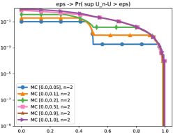
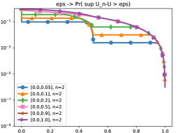
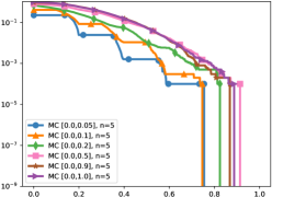
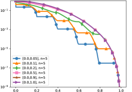
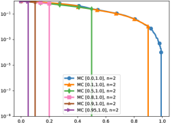
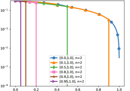
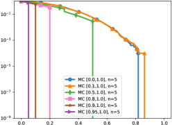
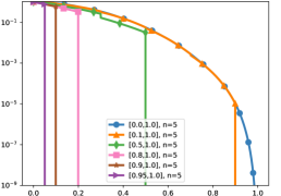
Figure 5: MCMC (left) versus Exact (Right) plot of $\varepsilon\to\delta_{[\underline{u},\overline{u}]}(n,\varepsilon)$ for various values of $n$ and interval $[\underline{u},\overline{u}]$ build from $M=10^{4}$ replicate.

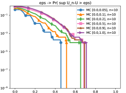
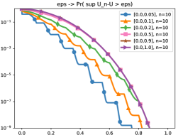
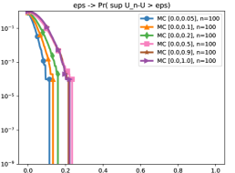
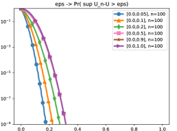
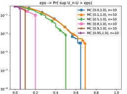
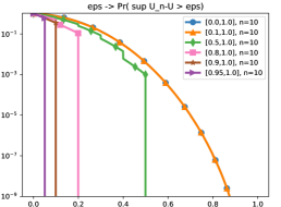
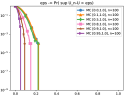
Figure 6: MCMC (left) versus Exact (Right) plot of $\varepsilon\to\delta_{[\underline{u},\overline{u}]}(n,\varepsilon)$ for various values of $n$ and interval $[\underline{u},\overline{u}]$ build from $M=10^{4}$ replicate.

In Figure 2, we plot $\varepsilon\to\delta_{[\underline{u},\overline{u}]}(n,\varepsilon)$ for various intervals $[\underline{u},\overline{u}]$, and in Figure 3, we plot $\varepsilon\to\tilde{\delta}_{[\underline{u},\overline{u}]}(n,\varepsilon)$. The plots highlight the non-trivial behavior of these functions, especially for small values of $n$, having plateaus, abrupt changes and non-linear behavior. These functions become smoother as $n$ increases (which is expected). Let us note the striking impact of changing $[\underline{u},\overline{u}]$ on the resulting function. In Appendix B, we further provide in Figure 5 and Figure 6 a numerical comparison between the computation of the exact probabilities from Theorem 3, and direct Monte Carlo simulations of the bound. The plots were obtained using $M=10^{4}$ simulations (we consider that the accuracy of such plots is hence good enough for values not less than $10^{-3}$), and perfectly match the theoretical bounds, as expected.

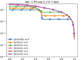
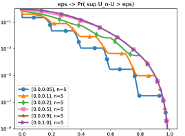
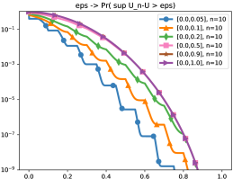
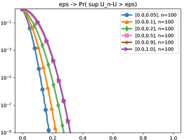
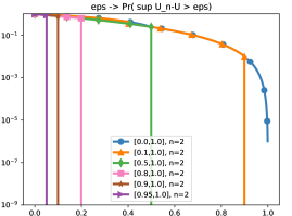
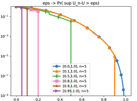
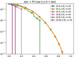
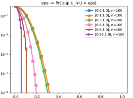
Figure 2: Plot of $\varepsilon\to\delta_{[\underline{u},\overline{u}]}(n,\varepsilon)$ for various values of $n$ and interval $[\underline{u},\overline{u}]$.

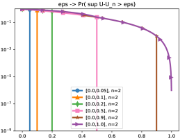
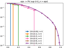
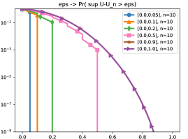
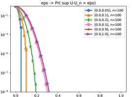
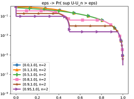
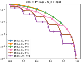
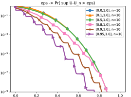
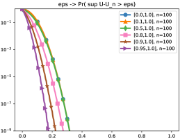
Figure 3: Plot of $\varepsilon\to\tilde{\delta}_{[\underline{u},\overline{u}]}(n,\varepsilon)$ for various values of $n$ and interval $[\underline{u},\overline{u}]$.

In Figure 4, we plot the inverse function $\delta\to\varepsilon_{[\underline{u},\overline{u}]}(n,\delta)$ as well as the explicit approximation given by Massart of the inverse probability function $\varepsilon_{[0,1]}$ for comparison. More precisely, we plot $\varepsilon(n,\delta)=\min\big{\{}\sqrt{\frac{\log(1/\delta)}{2n}},1\}$, simply called “DKW” in the plots (let us recall this function is only shown to control the deviations provided that $\delta\in[0,0.5)$, but this does not prevent us from plotting it for $[0,1]$). From the perspective of confidence bands, we believe that this function is the most interesting to plot, as it shows the exact magnitude of the estimation errors, and as such are not improvable. The plots confirm that the Massart bound is a valid upper bound on the exact probability functions, as can be seen by comparing in each plot the curve called DKW with the one obtained for the full set $[0,1]$. On the other hand, we also observe that this convenient but simplified bound can be quite conservative when considering a local supremum as opposed to a supremum over $[0,1]$. Also, the plots confirm that a simple expression cannot be obtained to accurately describe the behavior of $\varepsilon_{[\underline{u},\overline{u}]}$. The simplified bound provided by Massart is in this sense an especially convenient tool to trade-off accuracy and simplicity of the expression. However, we recommend using the exact bounds out of tightness, especially when the number of considered samples $n$ is small. Indeed in that case, the numerical cost of computing the exact bound should not be high.

Interestingly, we remark that a computation of $\varepsilon_{[\underline{u},\overline{u}]}$ and $\tilde{\varepsilon}_{[\underline{u},\overline{u}]}$ can be achieved numerically (hence, yielding the different plots) and readily translates into confidence bands over the local supremum deviation, offering tighter bounds for the practitioner. The computation of $\varepsilon_{[\underline{u},\overline{u}]}$ can further be done simply, e.g. by dichotomous search, in an efficient way up to a desired precision $\eta$. For instance Figure 4 has been obtained using precision $\eta=10^{-7}$. We believe this is a key point, as it indicates one can use such bounds in various applications, at a controlled computational cost. Note also that one can tabulate this function off-line, which is convenient for applications involving sequential decisions with increasingly many observations.

For ease of use, we provide for the interested reader the implementation details in the gitlab repository that is available at https://gitlab.inria.fr/omaillar/article-companion/-/tree/

master/2020-local-dkw. In order to avoid some numerical instabilities, the code uses a simple trick to replace expressions such as $x^{\ell}$ by $\exp(\ell\log(x))$. It also enables to reproduce all the plots displayed in the different figures of this article. Further, we provided a method to tabulate the inverse functions $\varepsilon_{[\underline{u},\overline{u}]}$ and $\tilde{\varepsilon}_{[\underline{u},\overline{u}]}$ for any given sub-interval of $[0,1]$, number of observations $n$ and given probability level $\delta$, which we believe to be useful for the practitioner.

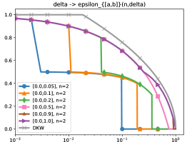
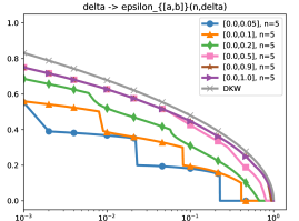
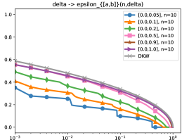
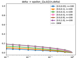
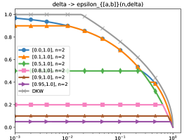
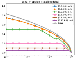
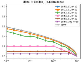
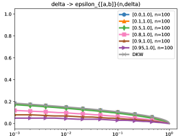
Figure 4: Plot of $\delta\to\varepsilon_{[\underline{u},\overline{u}]}(n,\delta)$ for various values of $n$ and intervals $[\underline{u},\overline{u}]$.

4 Application to the CVAR and other functionals of the CDF

In this section, we first introduce some background material and intuition about the risk measure known as the conditional value-at-risk (CVaR). For a probability distribution $\nu\in\mathcal{P}(\mathcal{X})$ taking values in $\mathcal{X}\subset\mathbb{R}$, let $\mathbb{E}_{\nu}$ denote its expectation operator and $F:x\mapsto\mathbb{P}_{\nu}(X\leqslant x)$ its Cumulative Distribution Function (CDF). Given $\alpha$, chosen by the practitioner, one may want to measure a risk using $\mathbb{E}_{\nu}[X|X<x_{\alpha}]$ for some $x_{\alpha}\in\mathcal{X}$ such that $F(x_{\alpha})=\alpha$ in case $X$ is a variable we want to maximize (reward), or $\mathbb{E}_{\nu}[X|X>x_{\kappa}]$ for some $x_{\kappa}\in\mathcal{X}$ such that $F(x_{\kappa})=\kappa$ in case $X$ is a variable we want to minimize (loss). Unfortunately, when $F$ is not continuously increasing, the points $x_{\alpha},x_{\kappa}$ may not exist. This is typically the case when $\nu=\nu_{n}$ is the empirical distribution built from $n$ observation. One way to overcome this problem is to introduce the Left Tail Conditional Expectation $\overline{\texttt{LTCE}}_{\alpha}(\nu)=\mathbb{E}_{\nu}\bigg{[}X\bigg{|}X\leqslant\overline{x}_{\alpha}(\nu)\bigg{]}$ together with the upper Value at Risk $\overline{x}_{\alpha}(\nu)=\inf\{x\in\mathbb{R}:F(x)>\alpha\}$, or the Right Tail Conditional Expectation $\underline{\texttt{RTCE}}_{\kappa}(\nu)=\mathbb{E}_{\nu}\bigg{[}X\bigg{|}X>\underline{x}_{\kappa}(\nu)\bigg{]}$ together with the lower Value at Risk $\underline{x}_{\kappa}(\nu)=\inf\{x\in\mathbb{R}:F(x)\geqslant\kappa\}$. Unfortunately, since in general $F(\overline{x}_{\alpha}(\nu))\geqslant F(\underline{x}_{\alpha}(\nu))\geqslant\alpha$ without equality, this makes such quantities difficult to interpret. The idea behind the classical definition of the CVaR is hence to interpolate between the values of $F$ around $\alpha$, using the following optimization problems (Rockafellar and Uryasev (2000))

$$\texttt{CVaR}^{r}_{\alpha}(\nu)=\sup_{x\in\mathbb{R}}\bigg{\{}\frac{1}{\alpha}\mathbb{E}[\min(X\!-\!x,0)]+x\bigg{\}}\,,\qquad\texttt{CVaR}^{\ell}_{\kappa}(\nu)=\inf_{x\in\mathbb{R}}\bigg{\{}x+\frac{1}{1-\kappa}\mathbb{E}[\max(X\!-\!x,0)]\bigg{\}}\,.$$

Let $X$ be a non negative random variable upper bounded by $\overline{x}$ for which $F$ is increasing and continuous. Then the following is known (see e.g. Acerbi (2002), or Thomas and Learned-Miller (2019); we reproduce this result in Appendix C for completeness)

Proposition 7 (CVaR to CDF reduction)

The quantity $\underline{x}_{\kappa}(\nu)$ is a solution to the $\texttt{CVaR}^{\ell}_{\kappa}$ optimization problem, and the following rewriting holds

$$\texttt{CVaR}^{\ell}_{\kappa}(\nu) \!=\! \frac{1}{1\!-\!\kappa}\mathbb{E}_{\nu}\Big{[}X\mathbb{I}\{X\!>\!\underline{x}_{\kappa}(\nu)\}\Big{]}=\underline{\texttt{RTCE}}_{\kappa}(\nu)=\overline{x}\!-\!\frac{1}{1\!-\!\kappa}\int_{0}^{\overline{x}}(F(x)\!-\!\kappa)_{+}dx\,.$$

$$\texttt{CVaR}^{r}_{\alpha}(\nu) \!=\! \frac{1}{\alpha}\mathbb{E}_{\nu}\Big{[}X\mathbb{I}\{X\!\leqslant\!\overline{x}_{\alpha}(\nu)\}\Big{]}=\overline{\texttt{LTCE}}_{\alpha}(\nu)=\frac{1}{\alpha}\int_{0}^{\overline{x}}(\alpha-F(x))_{+}dx\,.$$

In particular the CVaR writes as a function of the CDF in the form $\texttt{CVaR}^{r}_{\alpha}(\nu)=h^{r}\Big{(}\int_{\mathcal{X}}g^{r}\big{(}F(x)\big{)}dx\Big{)}$, where $h^{r}$ and $g^{r}$ are monotonic functions. Further $g^{r}(\beta)=(\alpha-\beta)_{+}$ has support $[0,\alpha)$ that is a strict subset of $[0,1]$ for $\alpha<1$. This property is actually not limited to the CVaR and allows to focus on controlling the deviations of the CDF to later control the risk-measure. Indeed, one can then build the confidence bands

$$\texttt{CVaR}_{\alpha,n,\delta}^{r,\pm}=h^{r}\Big{(}\int_{\mathcal{X}}g^{r}\big{(}F_{n}(x)\pm\varepsilon_{[0,\alpha]}(n,\delta)\big{)}dx\Big{)}\,.$$

Functional of the CDF

We now present a generalization of this procedure to other functionals of the CDF. In the sequel, we let $\mathcal{S}_{J}=\bigg{\{}\alpha=(\alpha_{0},\dots,\alpha_{J}),\alpha_{0}=0<\alpha_{1}<\dots<\alpha_{J}=1\}$ denote the set of increasing sequences partitioning the interval $[0,1]$ into $J$ segments. Further, for $\beta\in\mathcal{S}_{J}$, we let $\mathcal{S}_{K}(\beta)=\bigg{\{}\alpha\in\mathcal{S}_{K}:\exists k_{0}<k_{1},\dots<k_{J}\text{ s.t.}\alpha_{k_{j}}=\beta_{j}\bigg{\}}$. We now introduce a definition for convenience.

Definition 8 (Locally right-Lipschitz function)

A function $\varphi$ is locally lower-right-Lipschitz if it satisfies

$$\exists J\in\mathbb{N}_{\star},\beta\in\mathcal{S}_{J},\ell\in\mathbb{R}_{+}^{J}\,\,\forall j\in\{1,\dots,J\}\forall y\in[\beta_{j-1},\beta_{j}],\quad\forall\varepsilon>0,\frac{\varphi(y)-\varphi(y+\varepsilon)}{\varepsilon}\leqslant\ell_{j}\,.$$

A function $\varphi$ is locally upper-left-Lipschitz if it satisfies

$$\exists J\in\mathbb{N}_{\star},\beta\in\mathcal{S}_{J},\ell\in\mathbb{R}_{+}^{J}\,\,\forall j\in\{1,\dots,J\}\forall y\in[\beta_{j-1},\beta_{j}],\quad\forall\varepsilon>0,\frac{\varphi(y-\varepsilon)-\varphi(y)}{\varepsilon}\leqslant\ell_{j}\,.$$

For illustration, let us remark that $\texttt{CVaR}^{\ell}_{\kappa}(\nu)=\int_{\mathcal{X}}\varphi(F(x))dx$ with $\varphi(y)=1-\left(\frac{y-\kappa}{1-\kappa}\right)_{+}$. This non-increasing function is locally upper-left Lipschitz with $J=2$, $\beta=(0,\kappa,1)$ and $\ell=(0,\frac{1}{1-\kappa})$. On the other hand, $\texttt{CVaR}^{r}_{\alpha}(\nu)=\int_{\mathcal{X}}\varphi(F(x))dx$ with $\varphi(y)=\left(\frac{\alpha-y}{\alpha}\right)_{+}$. This non-increasing function is locally lower-right Lipschitz with $J=2$, $\beta=(0,\alpha,1)$ and $\ell=(\frac{1}{\alpha},0)$. This motivates the following result.

Theorem 9 (Functional of continuous CDF deviation)

For a distribution on $\mathcal{X}$ with continuous CDF $F$, let $\mu=\int_{\mathcal{X}}\varphi(F(x))dx$, where $\varphi$ is assumed to be a known, non-increasing function. For any $K\in\mathbb{N},\alpha\in\mathcal{S}_{k}$ and all $\delta_{k}\in[0,1],k\in\{1,\dots,K\}$ it holds that

$$\mathbb{P}\bigg{(}\mu<\sum_{k=0}^{K-1}\int_{\underline{x}_{\alpha_{k}}}^{\underline{x}_{\alpha_{k+1}}}\varphi\Big{(}\widehat{F}_{n}(x)+\tilde{\varepsilon}_{[\alpha_{k},\alpha_{k+1}]}(n,\delta_{k})\Big{)}\bigg{)} \leqslant \sum_{k=1}^{K}\delta_{k}\,,$$

$$\mathbb{P}\bigg{(}\mu>\sum_{k=0}^{K-1}\int_{\underline{x}_{\alpha_{k}}}^{\underline{x}_{\alpha_{k+1}}}\varphi\Big{(}\widehat{F}_{n}(x)-\varepsilon_{[\alpha_{k},\alpha_{k+1}]}(n,\delta_{k})\Big{)}\bigg{)} \leqslant \sum_{k=1}^{K}\delta_{k}\,,$$

where $\underline{x}_{\kappa}=\inf\{x\in\mathbb{R}:F(x)\geqslant\kappa\}$. Further, when $\varphi$ is locally lower-right Lipschitz with known $(J,\beta,\ell)$ and the quantile function $\kappa\mapsto\underline{x}_{\kappa}$ is $\gamma$-Lipschitz, then if $\alpha\in\mathcal{S}_{K}(\beta)$, the following holds

$$\mathbb{P}\bigg{(}\mu<\int_{\mathcal{X}}\varphi(\widehat{F}_{n}(x))dx-\sum_{j=1}^{J}\ell_{j}\sum_{k=k_{j-1}}^{k_{j}-1}\gamma(\alpha_{k+1}-\alpha_{k})\tilde{\varepsilon}_{[\alpha_{k},\alpha_{k+1}]}(n,\delta_{k})\bigg{)}\leqslant\sum_{k=1}^{K}\delta_{k}\,.$$

If instead $\varphi$ is locally upper-left Lipschitz with known $(J,\beta,\ell)$ and $\alpha\in\mathcal{S}_{K}(\beta)$, then

$$\mathbb{P}\bigg{(}\mu>\int_{\mathcal{X}}\varphi(\widehat{F}_{n}(x))dx+\sum_{j=1}^{J}\ell_{j}\sum_{k=k_{j-1}}^{k_{j}-1}\gamma(\alpha_{k+1}-\alpha_{k})\varepsilon_{[\alpha_{k},\alpha_{k+1}]}(n,\delta_{k})\bigg{)}\leqslant\sum_{k=1}^{K}\delta_{k}\,.$$

We only stated the result for a non-increasing function $\varphi$. Alternative results for a non-decreasing function and corresponding upper-right or lower-left assumptions can be derived too.

Proof of Theorem 9:

Indeed, first, using the definition of $\mu$ an the monotony of $\varphi$, it holds for all $\alpha\in\mathcal{S}_{K}(\beta)$

$$\mu = \sum_{k=0}^{K-1}\int_{\underline{x}_{\alpha_{k}}}^{\underline{x}_{\alpha_{k+1}}}\varphi\Big{(}\widehat{F}_{n}(x)+F(x)-\widehat{F}_{n}(x)\Big{)}dx$$

$$\geqslant \sum_{k=0}^{K-1}\int_{\underline{x}_{\alpha_{k}}}^{\underline{x}_{\alpha_{k+1}}}\varphi\Big{(}\widehat{F}_{n}(x)+\sup_{\underline{x}_{\alpha_{k}}\leqslant x\leqslant\underline{x}_{\alpha_{k+1}}}F(x)-\widehat{F}_{n}(x)\Big{)}dx$$

Now, using that $\sup_{\underline{x}_{\alpha_{k}}\leqslant x\leqslant\underline{x}_{\alpha_{k+1}}}F(x)-\widehat{F}_{n}(x)\stackrel{{\scriptstyle\mathcal{L}}}{{=}}\sup_{\alpha_{k}\leqslant u\leqslant\alpha_{k+1}}U(u)-\widehat{U}_{n}(u)$, we get that

$$\mu \stackrel{{\scriptstyle\mathcal{L}}}{{\geqslant}} \sum_{k=0}^{K-1}\int_{\underline{x}_{\alpha_{k}}}^{\underline{x}_{\alpha_{k+1}}}\varphi\Big{(}\widehat{F}_{n}(x)+\sup_{\alpha_{k}\leqslant u\leqslant\alpha_{k+1}}U(u)-\widehat{U}_{n}(u)\Big{)}dx$$

$$\geqslant \sum_{k=0}^{K-1}\int_{\underline{x}_{\alpha_{k}}}^{\underline{x}_{\alpha_{k+1}}}\varphi\Big{(}\widehat{F}_{n}(x)+\tilde{\varepsilon}_{[\alpha_{k},\alpha_{k+1}]}(n,\delta_{k})\Big{)}dx\,.$$

where the last inequality holds on an event of probability higher than $1-\sum_{k=1}^{K}\delta_{k}$. Last, using the local Lipschitz property, we get

$$\mathbb{P}\bigg{(}\mu<\int_{\mathcal{X}}\varphi\big{(}\widehat{F}_{n}(x)\big{)}-\sum_{j=1}^{J}\ell_{j}\sum_{k=k_{j-1}}^{k_{j}-1}(\underline{x}_{\alpha_{k+1}}-\underline{x}_{\alpha_{k}})\tilde{\varepsilon}_{[\alpha_{k},\alpha_{k+1}]}(n,\delta_{k})\bigg{)}\leqslant\sum_{k=1}^{K}\delta_{k}\,.$$

We conclude using the assumption that $F$ has $\gamma$-Lipshitz quantile function. $\hfill\square$

5 Time-uniform concentration inequalities

In this section, we now provide an extension of the previous result and focus on the number of samples $n$. The previous result provide a confidence bound valid with high probability for each $n$. In some situations, one way want to have a high probability control valid simultaneously for all $n$ in a given range, or even simultaneously all $n\in\mathbb{N}$. In order to derive such bounds, classical techniques consists of using (1) a union bound argument, (2) a geometric time-peeling argument together with Doob’s maximal inequality for sub-martingales, or (3) a method of mixture (Laplace method) for specific distributions. These techniques lead to different bounds, the union bound technique being the simplest yet yielding the largest time-uniform confidence bands. In the following, we provide a version of the geometric time-peeling argument for the control of the supremum CDF. One difficulty is that a Martingale cannot be easily built in this case, and hence we replace the use of Doob’s maximal inequality with a weaker reflection inequality that can be traced back at least to James (1975).

We first show below a slight extension of (Shorack and Wellner, 2009, Inequality 13.2.1) (the result from Shorack and Wellner (2009) itself originates from, and slightly extends that of James (1975)). The proof of this result easily follows by looking at inequality (a) p. 513 in the proof of (Shorack and Wellner, 2009, Inequality 13.2.1) and thus is not reproduced here.

Lemma 10 (Reflection inequality)

Let $\eta\!>\!1,\lambda\!>\!0$ and then $\underline{u},\overline{u}\!\in\![0,1]$. Let $c\!\in\!(0,1)$ be such that $\frac{(C-1)(1-c)^{2}\lambda^{2}}{C(\eta\!-\!1)}\geqslant\sup_{x\in[\underline{u},\overline{u}]}x(1-x)$ for some $C>1$ Then, for all integers $n_{1},n_{2}\!\in\!\mathbb{N}$ such that $n_{2}\!\leqslant n_{1}\!\eta$, it holds

$$\mathbb{P}\bigg{(}\max_{n_{1}\leqslant n\leqslant n_{2}}\sup_{x\in[\underline{u},\overline{u}]}\sqrt{n}\Big{(}U_{n}(x)-U(x)\Big{)}>\lambda\bigg{)} \leqslant C\mathbb{P}\bigg{(}\sup_{x\in[\underline{u},\overline{u}]}\sqrt{n_{2}}\Big{(}U_{n_{2}}(x)-U(x)\Big{)}>\frac{c}{\sqrt{\eta}}\lambda\bigg{)}\,.$$

$$\mathbb{P}\bigg{(}\max_{n_{1}\leqslant n\leqslant n_{2}}\sup_{x\in[\underline{u},\overline{u}]}\sqrt{n}\Big{(}U(x)-U_{n}(x)\Big{)}>\lambda\bigg{)} \leqslant C\mathbb{P}\bigg{(}\sup_{x\in[\underline{u},\overline{u}]}\sqrt{n_{2}}\Big{(}U(x)-U_{n_{2}}(x)\Big{)}>\frac{c}{\sqrt{\eta}}\lambda\bigg{)}\,.$$

We deduce from this key result the following maximal inequality

Corollary 11 (Maximal inequality)

Let $\eta\!>\!1$, $C\!>\!1$, $\underline{u},\overline{u}\!\in\![0,1]$ then $q\!=\!\sup_{x\in[\underline{u},\overline{u}]}x(1-x)$. For any $n_{1},n_{2}\!\in\!\mathbb{N}$ such that $n_{2}\!\leqslant\!\eta n_{1}$ and for any $\varepsilon>0$ such that $\varepsilon>\sqrt{\frac{Cq(\eta\!-\!1)}{(C-1)n_{1}}}$, it comes

$$\mathbb{P}\bigg{(}\max_{n_{1}\leqslant n\leqslant n_{2}}\sup_{x\in[\underline{u},\overline{u}]}U_{n}(x)\!-\!U(x)>\varepsilon\bigg{)} \leqslant C\mathbb{P}\bigg{(}\sup_{x\in[\underline{u},\overline{u}]}U_{n_{2}}(x)\!-\!U(x)>\sqrt{\frac{n_{1}}{n_{2}\eta}}\Big{(}\varepsilon\!-\!\sqrt{\frac{Cq(\eta\!-\!1)}{(C-1)n_{1}}}\Big{)}\bigg{)}\,.$$

$$\mathbb{P}\bigg{(}\max_{n_{1}\leqslant n\leqslant n_{2}}\sup_{x\in[\underline{u},\overline{u}]}U(x)\!-\!U_{n}(x)>\varepsilon\bigg{)} \leqslant C\mathbb{P}\bigg{(}\sup_{x\in[\underline{u},\overline{u}]}U(x)\!-\!U_{n_{2}}(x)>\sqrt{\frac{n_{1}}{n_{2}\eta}}\Big{(}\varepsilon\!-\!\sqrt{\frac{Cq(\eta\!-\!1)}{(C-1)n_{1}}}\Big{)}\bigg{)}\,.$$

Proof of Corollary 11:

First, we successively derive

$$\mathbb{P}\bigg{(}\max_{n_{1}\leqslant n\leqslant n_{2}}\sup_{x\in[\underline{u},\overline{u}]}U_{n}(x)-U(x)>\varepsilon\bigg{)} \leqslant \mathbb{P}\bigg{(}\max_{n_{1}\leqslant n\leqslant n_{2}}\sup_{x\in[\underline{u},\overline{u}]}\frac{\sqrt{n}}{\sqrt{n_{1}}}\Big{(}U_{n}(x)-U(x)\Big{)}>\varepsilon\bigg{)}$$

$$= \mathbb{P}\bigg{(}\max_{n_{1}\leqslant n\leqslant n_{2}}\sup_{x\in[\underline{u},\overline{u}]}\sqrt{n}\Big{(}U_{n}(x)-U(x)\Big{)}>\sqrt{n_{1}}\varepsilon\bigg{)}$$

$$\leqslant C\mathbb{P}\bigg{(}\sup_{x\in[\underline{u},\overline{u}]}\sqrt{n_{2}}\Big{(}U_{n_{2}}(x)-U(x)\Big{)}>\sqrt{\frac{n_{1}}{\eta}}\varepsilon c\bigg{)}\,.$$

Note that in the first line, we considered the event that $\sup_{x}U_{n}(x)-U(x)>0$. Indeed the complementary event does not intersect the event of interest. Now, we choose for $c\in(0,1)$ the maximal value such that $\frac{n_{1}(C-1)(1-c)^{2}\varepsilon^{2}}{C(\eta\!-\!1)}\geqslant\sup_{x\in[\underline{u},\overline{u}]}x(1-x)$, that is $c=1-\frac{\sqrt{C(\eta\!-\!1)q}}{\sqrt{(C-1)n_{1}}\varepsilon}$, provided that $\sqrt{\frac{C(\eta\!-\!1)q}{(C-1)n_{1}}}<\varepsilon$. Reorganizing the terms yields the conclusion. We proceed similarly for the second inequality. $\hfill\square$

We are now ready to prove Theorem 12. To this end, we combine Corollary 11 together with the local DKW inequality, on top of the standard geometric time-peeling technique.

Theorem 12 (Time-Uniform local DKW inequality)

Let $n\!\in\!\mathbb{N}$, and consider any random stopping time $N_{n}$ a.s. upper-bounded by $n$. Let us introduce a function $\varepsilon_{[\underline{u},\overline{u}]}$ such that

$$\forall\delta\!\in\!(0,1),\forall n\!\in\!\mathbb{N},\quad\mathbb{P}\bigg{(}\sup_{x\in[\underline{u},\overline{u}]}U_{n}(x)-U(x)>\varepsilon_{[\underline{u},\overline{u}]}\Big{(}n,\delta\Big{)}\bigg{)}\leqslant\delta\,.$$

Then for all $\eta>1$, for all $\delta_{n}\in(0,1)$, and $C>1$, it holds

$$\mathbb{P}\bigg{(}\!\sup_{x\in[\underline{u},\overline{u}]}U_{N_{n}}(x)\!-\!U(x)>\frac{1}{\sqrt{N_{n}\!-\!(\eta\!-\!1)}}\Big{[}\eta\sqrt{N_{n}}\varepsilon_{[\underline{u},\overline{u}]}\bigg{(}\!N_{n},\frac{\delta_{n}/C}{\big{\lceil}\frac{\log(n)}{\log(\eta)}\big{\rceil}}\!\bigg{)}+\sqrt{\!\frac{C}{C\!-\!1}q\eta(\eta\!-\!1)}\Big{]}\bigg{)}\leqslant\delta_{n}\,.$$

Likewise, if $\tilde{\varepsilon}_{[\underline{u},\overline{u}]}$ controls $\sup_{x\in[\underline{u},\overline{u}]}U(x)-U_{n}(x)$, a similar inequality holds replacing $U_{n}(x)-U(x)$ with $U(x)-U_{n}(x)$ and $\varepsilon_{[\underline{u},\overline{u}]}$ with $\tilde{\varepsilon}_{[\underline{u},\overline{u}]}$.

Corollary 13 (Time-Uniform global DKW inequality)

In particular for $[\underline{u},\overline{u}]=[0,1]$, choosing $C=2$, and using that $q\leqslant 1/4$ it comes $\forall\delta\in(0,0.5)$,

$$\mathbb{P}\bigg{(}\sup_{x\in[0,1]}U_{N_{n}}(x)-U(x)>\frac{1}{\sqrt{2(N_{n}-(\eta\!-\!1))}}\Big{[}\eta\sqrt{\log\bigg{(}\bigg{\lceil}\frac{\log(n)}{\log(\eta)}\bigg{\rceil}\frac{2}{\delta}\bigg{)}}+\sqrt{\eta(\eta\!-\!1)}\Big{]}\bigg{)}\leqslant\delta\,.$$

Corollary 13 is stated for convenience, to show an explicit formula that can be used to control uniform deviations uniformly over time. This result should be compared to the term $\sqrt{\log(1/\delta)/2n}$ obtained for a single $n$ by application of Massart’s inequality. Note the $\log\log(n)$ scaling, compared to the $\log(n)$ term one would obtain from a simple union bound.

Proof of Theorem 12:

Let us introduce $t_{k}=\lfloor\eta^{k}\rfloor$, for $k=0,\dots,K$ with $K=\big{\lceil}\frac{\log(n)}{\log(\eta)}\big{\rceil}$ (thus $n\leqslant t_{K}$), for some constant $\eta>1$. Let also $\varepsilon$ be a non-increasing positive function on $\mathbb{R}$, to be defined later.

$$\mathbb{P}\bigg{(}\sup_{x\in[\underline{u},\overline{u}]}U_{N_{n}}(x)-U(x)>\varepsilon(N_{n})\bigg{)}$$

$$\leqslant \sum_{k=1}^{K}\mathbb{P}\bigg{(}\exists t\in[t_{k\!-\!1},t_{k}\!-\!1]:\sup_{x\in[\underline{u},\overline{u}]}\Big{(}U_{t}(x)-U(x)\Big{)}>\varepsilon(t)\bigg{)}$$

$$\leqslant \sum_{k=1}^{K}\mathbb{P}\bigg{(}\max_{t\in[t_{k\!-\!1},t_{k}\!-\!1]}\sup_{x\in[\underline{u},\overline{u}]}\Big{(}U_{t}(x)-U(x)\Big{)}>\varepsilon(t_{k}-1)\bigg{)}$$

$$\leqslant \sum_{k=1}^{K}C\mathbb{P}\bigg{(}\sup_{x\in[\underline{u},\overline{u}]}\Big{(}U_{t_{k}-1}(x)-U(x)\Big{)}>\sqrt{\frac{t_{k-1}}{(t_{k}-1)\eta}}\Big{(}\varepsilon(t_{k}\!-\!1)-\sqrt{\frac{Cq(\eta\!-\!1)}{(C\!-\!1)t_{k-1}}}\Big{)}\bigg{)}$$

In order to make use of local DKW inequality, let us choose the function $\varepsilon$ such that

$$\sqrt{\frac{t_{k-1}}{(t_{k}-1)\eta}}\Big{(}\varepsilon(t_{k}\!-\!1)-\sqrt{\frac{Cq(\eta\!-\!1)}{(C\!-\!1)t_{k-1}}}\Big{)}\geqslant\varepsilon_{[\underline{u},\overline{u}]}(t_{k}\!-\!1,\delta_{k})\,.$$

Indeed, this ensures by local DKW inequality that, provided that $\delta_{k}\in(0,1)$,

$$\mathbb{P}\bigg{(}\sup_{x\in[\underline{u},\overline{u}]}\Big{(}U_{N_{n}}(x)-U(x)\Big{)}>\varepsilon(N_{n})\bigg{)}\leqslant\sum_{k=1}^{K}C\delta_{k}\,,$$

and assuming $C>1$, we can further choose $\delta_{k}=\delta/(CK)$ for $\delta\in(0,1)$. That is, we want

$$\varepsilon(t_{k}\!-\!1)\geqslant\frac{1}{\sqrt{t_{k-1}}}\bigg{(}\sqrt{(t_{k}-1)\eta}\varepsilon_{[\underline{u},\overline{u}]}\Big{(}t_{k}\!-\!1,\frac{\delta}{CK}\Big{)}+\sqrt{\frac{C}{C\!-\!1}q(\eta\!-\!1)}\bigg{)}$$

We now use the fact that

$$t_{k}-1 = \lfloor\eta^{k}\rfloor-1\leqslant\eta^{k-1}\eta-1=\lfloor\eta^{k-1}\rfloor\eta+\Big{(}\eta^{k-1}-\lfloor\eta^{k-1}\rfloor\Big{)}\eta\!-\!1$$

$$\leqslant t_{k-1}\eta+(\eta\!-\!1)\,.$$

Hence, we conclude the proof by choosing the function

$$\varepsilon(t) = \sqrt{\frac{\eta}{t-(\eta\!-\!1)}}\Big{(}\sqrt{t\eta}\varepsilon_{[\underline{u},\overline{u}]}(t,\frac{\delta}{CK})+\sqrt{\frac{C}{C\!-\!1}q(\eta\!-\!1)}\Big{)}$$

$$= \frac{1}{\sqrt{t-(\eta\!-\!1)}}\Big{(}\eta\sqrt{t}\varepsilon_{[\underline{u},\overline{u}]}(t,\frac{\delta}{CK})+\sqrt{\frac{C}{C\!-\!1}q\eta(\eta\!-\!1)}\Big{)}\,.$$

$\hfill\square$

An application to the cumulative control of sequential deviations

Using Theorem 12, we deduce the following control, together with tuning recommendations for the practitioner.

Corollary 14 (Time uniform cumulative error control)

Let $q=\sup_{x\in[\underline{u},\overline{u}]}x(1-x)$. Let $(\eta_{t})_{t}$ be a decreasing sequence converging to $1$, and $(\delta_{t})_{t}\subset(0,1)$. Then, it holds

$$\sum_{t=1}^{T}\mathbb{P}\bigg{(}\sup_{x\in[\underline{u},\overline{u}]}U_{N_{t}}(x)-U(x) > \frac{1}{\sqrt{N_{t}\!-\!(\eta_{t}\!-\!1)}}\Big{[}\eta_{t}\sqrt{N_{t}}\varepsilon_{[\underline{u},\overline{u}]}\bigg{(}N_{t},\delta_{t}\bigg{)}+\sqrt{2q\eta_{t}(\eta_{t}\!-\!1)}\Big{]}\bigg{)}$$

$$\leqslant 2\sum_{t=1}^{T}\bigg{\lceil}\frac{\log(t)}{\log(\eta_{t})}\bigg{\rceil}\delta_{t},$$

In particular, provided that (a) $\log(\eta_{t})^{-1}=O(\log^{\alpha}(t))$ for some $\alpha<1$, choosing $\delta_{t}$ such that $\log(t)^{2}\delta_{t}=O(1/t)$ ensures that the right hand side term is $o(\log(T))$. This quantity is also

$$o(\log(T)) \eta_{t}=\frac{f(t)+1}{f(t)}\text{ and }\delta_{t}=\exp(-f(t))\text{ where}f(t)=\log(t)+\xi\log\log(t)\text{ with }\xi>2\,.$$ for (b)

$$\leqslant 1 \delta_{t}=\bigg{\lceil}\frac{\log(t)}{\log(\eta_{t})}\bigg{\rceil}^{-1}\frac{1}{2g(t)}\text{ where }\sum_{t=1}^{\infty}\frac{1}{g(t)}\leqslant 1\text{ provided that }\delta_{t}\leqslant 1.$$ for (c)

Remark 15

The tuning of $\eta_{t}$ using $f(t)$ is the one suggested in Cappé et al. (2013) for the tuning of the KL-UCB algorithm, and this is the one we suggest using in practice. In the last case c), the condition $\delta_{t}\leqslant 1$ constrains the choice of $\eta_{t}$ that cannot be too small. In particular, it cannot converge too fast towards $1$. Some classical choice for $g$ include $g(t)=3t^{3/2}$, $g(t)=t(t+1)$ or $g(t)=(t+1)\log^{2}(t+1)/\log(2)$. See Appendix D for other possible choices for $g$.

Remark 16

For comparison, note that a union bound argument yields the alternative bound

$$\sum_{t=1}^{T}\mathbb{P}\bigg{(}\sup_{x\in[\underline{u},\overline{u}]}U_{N_{t}}(x)-U(x)>\varepsilon_{[\underline{u},\overline{u}]}(N_{t},\delta_{t})\bigg{)}\leqslant\sum_{t=1}^{T}t\delta_{t}\,,$$

which suggests choosing e.g. $\delta_{t}=(tg(t))^{-1}$. A classical choice is e.g. $\delta(t)=(t^{2}(t+1))^{-1}$.

Proof of Corollary 14:

We apply Theorem  12 with $C=2$ in order to get the claimed inequality.

The first claim follows from the fact that $\bigg{\lceil}\frac{\log(t)}{\log(\eta_{t})}\bigg{\rceil}\delta_{t}=O(t^{-1}\log(t)^{1+\alpha-2})=o(t^{-1})$ under the considered assumption.

Regarding the second claim, for the choice $\eta_{t}=\frac{f(t)+1}{f(t)}$ and $\delta_{t}=\exp(-f(t))$ where $f(t)=\log(t)+\xi\log\log(t)$, we obtain that

$$\sum_{t}\bigg{\lceil}\frac{\log(t)}{\log(\eta_{t})}\bigg{\rceil}\delta_{t} = e\sum_{t}\frac{1}{t\log^{\xi}(t)}\lceil\log^{2}(t)+\xi\log(t)\log\log(t)\rceil$$

$$\leqslant e\sum_{t}\frac{1}{t\log^{\xi-2}(t)}+e\sum_{t}\frac{\log\log(t)}{t\log^{\xi-1}(t)}+e\sum_{t}\frac{1}{t\log^{\xi}(t)}\,.$$

Hence, provided that $\xi>2$, this sum is $o(\log(T))$. The last claim is direct; note that the condition $\delta_{t}\leqslant 1$ constrains the choice of admissible $\eta_{t}$. $\hfill\square$

A Proofs of the main results

Proof of Lemma 2:

We let $[n]=\{1,\dots,n\}$ for all $n\in\mathbb{N}_{\star}$.

Left tail, step 1 Let first recall the following remark by Smirnov (Smirnov, 1944, p.10), showing that if $u_{(1)},\dots,u_{(n)}$ denotes the order samples received from the uniform distribution, then

$$\mathbb{P}(\sup_{u\in[0,1]}U_{n}(u)-u\leqslant\varepsilon) = \mathbb{P}\Big{(}\forall k\in[n],\quad U_{n}(u_{(k)})-\varepsilon\leqslant u_{(k)}\Big{)}$$ (1)

$$= \mathbb{P}\Big{(}\forall k\in[n],\quad k/n-\varepsilon\leqslant u_{(k)}\Big{)}$$

$$= n!\!\int\!\dots\!\int\!\mathbb{I}\bigg{\{}0\!\leqslant\!u_{1}\!\leqslant\!\dots u_{n}\!\leqslant\!1;\forall k,u_{k}\geqslant k/n-\varepsilon\bigg{\}}du_{1}\dots du_{n}\,.$$

When restricting the supremum to $[\alpha,\beta]$, this equality needs to be modified. First of all, it holds that

$$\sup_{u\in[\alpha,\beta]}U_{n}(u)-u=\max\bigg{\{}U_{n}(v)-v:v\in\{\alpha\}\cup\{u_{(1)},\dots,u_{(n)}\}\cap[\alpha,\beta]\bigg{\}}\,.$$

Hence, we deduce that

$$\bigg{\{}\sup_{u\in[\alpha,\beta]}U_{n}(u)-u\leqslant\varepsilon\bigg{\}}$$

$$= \bigcap_{k\in[n]}\bigg{\{}u_{(k)}\in[\alpha,\beta]\implies U_{n}(u_{(k)})-\varepsilon\leqslant u_{(k)}\bigg{\}}\cap\bigg{\{}U_{n}(\alpha)\leqslant\varepsilon+\alpha\bigg{\}}$$

$$= \bigcap_{k\in[n]}\bigg{\{}u_{(k)}\in[\alpha,\beta]\implies k/n-\varepsilon\leqslant u_{(k)}\bigg{\}}\cap\bigg{\{}\sum_{k=1}^{n}\mathbb{I}\{u_{(k)}\leqslant\alpha\}\leqslant n(\varepsilon+\alpha)\bigg{\}}$$

$$= \bigcap_{k\in[n]}\bigg{\{}u_{(k)}\in[\alpha,\beta]\implies k/n-\varepsilon\leqslant u_{(k)}\bigg{\}}\cap\bigg{\{}u_{(k)}\leqslant\alpha<u_{(k+1)}\implies k/n\leqslant\varepsilon+\alpha\bigg{\}}\,,$$

where we introduced the term $u_{(n+1)}=1$ in the last line and used that $\varepsilon+\alpha\geqslant 0$ to exclude the term $u_{(0)}=0$. Using the distribution of the order statistics, we deduce that

$$\mathbb{P}\Big{(}\sup_{u\in[\alpha,\beta]}U_{n}(u)-U(u)\leqslant\varepsilon\Big{)}$$

$$= \!\!n!\!\int\!\dots\!\int\!\mathbb{I}\bigg{\{}0\!\leqslant\!u_{1}\!\leqslant\!\dots u_{n}\!\leqslant\!1;\forall k\!\in\![n],\begin{cases}\text{if }u_{k}\!\in\![\alpha,\beta]&\text{ then }u_{k}\geqslant\frac{k}{n}-\varepsilon\\ \text{if }k\!>\!n(\varepsilon\!+\!\alpha)&\text{ then }\alpha\!\notin\![u_{k},u_{k+1})\\ \end{cases}\bigg{\}}du_{1}\dots du_{n}.$$

Left tail, step 2 Following Smirnov (1944), we introduce the notation $t_{k}=u_{n-k+1}$, constant $\gamma_{k}=(n-k+1)/n-\varepsilon$ (non-negative for $k\leqslant n-\lfloor\varepsilon n\rfloor$) as well as $\beta_{k}=\min(\gamma_{k},\beta)$. We thus have the following rewriting

$$\bigg{\{}t\in[0,1]:\text{if }t\in[\alpha,\beta]\text{ then }t\geqslant\gamma_{k}\bigg{\}} = [0,\alpha]\cup[\min(\gamma_{k},\beta),1]=[0,\alpha]\cup[\beta_{k},1]\,,$$

which further reduces to $[0,1]$ when $\gamma_{k}\leqslant\alpha$. We let $n_{\alpha,\varepsilon}=n(1\!-\!\varepsilon\!-\!\alpha)$, $\overline{n}_{\alpha,\varepsilon}=\lceil n_{\alpha,\varepsilon}\rceil$ and remark that $\gamma_{k}\leqslant\alpha$ iff $k\geqslant n_{\alpha,\varepsilon}+1$ . Also, $\gamma_{k}\leqslant\alpha$ as soon as $k>\overline{n}_{\alpha,\varepsilon}$. Let us also note that $n-k+1>n(\varepsilon+\alpha)$ iff $k<n_{\alpha,\varepsilon}+1$, and that $\overline{n}_{\alpha,\varepsilon}<n_{\alpha,\varepsilon}+1$. This means in particular that if $k\geqslant\overline{n}_{\alpha,\varepsilon}+1$, then both conditions in the integral vanish (so contribute to $1$ in the integral).

$$\mathbb{P}\Big{(}\sup_{u\in[\alpha,\beta]}U_{n}(u)-U(u)\leqslant\varepsilon\Big{)}$$

$$= \!\!n!\!\int\!\dots\!\int\!\!\mathbb{I}\bigg{\{}\!0\!\leqslant\!t_{n}\!\leqslant\!\dots t_{1}\!\leqslant\!1;\forall k\!\in\![n],t_{k}\!\in\![0,\alpha]\!\cup\![\beta_{k},1],\forall k\!\leqslant\!\overline{n}_{\alpha,\varepsilon},\alpha\!\notin\![t_{k},t_{k-1})\!\bigg{\}}dt_{n}\dots dt_{1}$$

$$= \!\!n!\!\!\int\!\dots\!\int\!\!\mathbb{I}\bigg{\{}\!0\!\leqslant\!t_{\overline{n}_{\alpha,\varepsilon}}\!\leqslant\!\dots t_{1}\!\leqslant\!1;$$

$$\qquad\qquad\forall k\!\leqslant\!\overline{n}_{\alpha,\varepsilon},t_{k}\!\in\![0,\alpha]\!\cup\![\beta_{k},\!1]\text{ and }\alpha\!\notin\![t_{k},t_{k-1})\!\!\bigg{\}}J_{n\!-\!\overline{n}_{\alpha,\varepsilon}}\!(t_{\overline{n}_{\alpha,\varepsilon}})dt_{\overline{n}_{\alpha,\varepsilon}\!}\!\dots dt_{1}\,,$$

where we integrated out all terms for $k>\overline{n}_{\alpha,\varepsilon}$ into the short-hand notation $J_{k}(x)=\frac{x^{k}}{k!}$. In the integral, we note that if $t_{k}\leqslant\alpha$, then so must be all terms $t_{k^{\prime}}$ for $k^{\prime}\geqslant k$.

We now proceed with integration. Starting with $t_{1}$, we see that if $t_{1}\leqslant\alpha$, then this implies $\alpha\in[t_{1},t_{0}]$. Hence, the corresponding terms are $0$, and it remains to integrate $t_{1}$ on $(\alpha,1]$, that is on $[\beta_{1},1]$.

Regarding $t_{2}$, if $t_{2}\leqslant\alpha<t_{1}$, this contradicts $\alpha\notin[t_{2},t_{1}]$, hence it remains it remains to integrate $t_{2}$ on $(\alpha,1]$, that is on $[\beta_{2},1]$. Proceeding similarly, for all $k\leqslant\overline{n}_{\alpha,\varepsilon}$ we obtain that

$$\mathbb{P}\Big{(}\sup_{u\in[\alpha,\beta]}U_{n}(u)-U(u)\leqslant\varepsilon\Big{)} = n!\int_{\beta_{1}}^{1}\!\int_{\beta_{2}}^{t_{1}}\!\dots\!\int_{\beta_{\overline{n}_{\alpha,\varepsilon}}}^{t_{\overline{n}_{\alpha,\varepsilon}-1}}\!\!J_{n-\overline{n}_{\alpha,\varepsilon}}(t_{\overline{n}_{\alpha,\varepsilon}})dt_{\overline{n}_{\alpha,\varepsilon}}\!\dots\!dt_{1}\!\,.$$

In order to compute the multiple integral, similarly to Smirnov (1944), we make use of the following variant of the Taylor expansion

$$f(x) = f(a_{1})+\sum_{\ell=1}^{n-k-1}f^{(\ell)}(a_{\ell+1})\int_{a_{1}}^{x}\int_{a_{2}}^{t_{1}}\dots\int_{a_{k}}^{t_{\ell-1}}dt_{1}\dots dt_{\ell}$$

$$+\int_{a_{1}}^{x}\int_{a_{2}}^{t_{1}}\dots\int_{a_{n-k}}^{t_{n-k-1}}f^{(n-k)}(t_{n-k})dt_{1}\dots dt_{n-k}\,,$$

which, using the $I_{k}$ notation, yields the following form

$$\int_{a_{1}}^{x}\int_{a_{2}}^{t_{1}}\dots\int_{a_{n-k}}^{t_{n-k-1}}f^{(n-k)}(t_{n-k})dt_{1}\dots dt_{n-k}=f(x)-f(a_{1})-\sum_{\ell=1}^{n-k-1}f^{(\ell)}(a_{\ell+1})I_{\ell}(x;a_{1},\dots,a_{\ell})\,.$$

This is applied to the function $f(x)=x^{n}$, $k=n-\overline{n}_{\alpha,\varepsilon}$. Indeed, we then get $f^{(n-k)}(x)=\frac{n!x^{k}}{k!}=\frac{n!x^{n-\overline{n}_{\alpha,\varepsilon}}}{(n-\overline{n}_{\alpha,\varepsilon})!}=n!J_{n-\overline{n}_{\alpha,\varepsilon}}(x)$. This in turns yields

$$\mathbb{P}\Big{(}\sup_{u\in[\alpha,\beta]}U_{n}(u)-U(u)\leqslant\varepsilon\Big{)} = 1-\beta_{1}^{n}-\sum_{\ell=1}^{\overline{n}_{\alpha,\varepsilon}-1}\frac{n!}{(n-\ell)!}\beta_{\ell+1}^{n-\ell}I_{\ell}(1;\beta_{1},\dots\beta_{\ell})$$

$$= 1-\sum_{\ell=0}^{\overline{n}_{\alpha,\varepsilon}-1}\binom{n}{\ell}\beta_{\ell+1}^{n-\ell}\ell!I_{\ell}(1;\beta_{1},\dots\beta_{\ell})\,,$$

using the convention that $I_{0}(x;\emptyset)=1$. This completes the proof regarding the left tail concentration.

Right tail We proceed similarly for the right tail. First, using our notation we note that

$$\sup_{u\in[\alpha,\beta]}U(u)-U_{n}(u)=\max\bigg{\{}\lim_{u\to v;u<v}U(u)-U_{n}(u):v\in\{\beta\}\cup\{u_{(1)},\dots,u_{(n)}\}\cap(\alpha,\beta]\bigg{\}}$$

To be more precise, we let $(\eta_{k})_{k\in[n]}>0$ be arbitrary small constants. We also let $\eta_{0}<\min_{k\in[n]}\eta_{k}$ and define $\overline{\eta}=\max_{k\in[n]}\eta_{k}$. We further introduce, for each $k\!\in\![n]$, $u^{-}_{(k)}$ such that $u_{(k)}-\eta=u^{-}_{(k)}<u_{(k)}$, and $\beta^{-}$ such that $\beta-\eta_{0}=\beta^{-}<\beta$. Then, we introduce the notation

$$\sup^{\eta}_{u\in[\alpha,\beta]}U(u)-U_{n}(u)=\max\bigg{\{}U(v)-U_{n}(v):v\in\{\beta^{-}\}\cup\{u_{(1)}^{-},\dots,u_{(n)}^{-}\}\cap(\alpha,\beta]\bigg{\}}\,.$$

Before proceeding, we note that $\forall n\!\in\!\mathbb{N},\lim_{\overline{\eta}\to 0}\mathbb{P}(\min_{k\in[n]}u_{(k)}-u_{(k-1)}>\eta_{k})=1$ Indeed, it holds

$$\mathbb{P}\big{(}\min_{k\in[n]}u_{(k)}-u_{(k-1)}\leqslant\eta_{k}\big{)} = \mathbb{P}\big{(}\exists{k\in[n]},\,\,u_{(k)}-u_{(k-1)}\leqslant\eta_{k}\big{)}$$

$$\leqslant \mathbb{P}\big{(}\exists{i,j\in[n],i<j},\,\,|X_{i}-X_{j}|\leqslant\overline{\eta}\big{)}$$

$$\leqslant \frac{n(n-1)}{2}\mathbb{P}(|X_{1}-X_{2}|\leqslant\overline{\eta})=n(n-1)\overline{\eta}\,.$$

In the following, we use a construction similar to that of Kolmogorov (1956) for Skorokhod convergence. Note that under the event that $\Omega_{n}=\big{\{}\min_{k\in[n]}u_{(k)}-u_{(k-1)}>\eta_{k}\big{\}}$ (where $u_{(0)}=0$) we have the following rewriting

$$\bigg{\{}\sup^{\eta}_{u\in[\alpha,\beta]}u-U_{n}(u)\leqslant\varepsilon\bigg{\}}$$

$$= \bigcap_{k\in[n]}\bigg{\{}u_{(k)}^{-}\in[\alpha,\beta]\implies u_{(k)}^{-}-\varepsilon\leqslant U_{n}(u_{(k)}^{-})\bigg{\}}\cap\bigg{\{}\beta^{-}-\varepsilon\leqslant U_{n}(\beta^{-})\bigg{\}}$$

$$= \bigcap_{k\in[n]}\bigg{\{}u_{(k)}^{-}\in[\alpha,\beta]\implies u_{(k)}^{-}-\varepsilon\leqslant(k-1)/n\bigg{\}}\cap\bigg{\{}\sum_{k=1}^{n}\mathbb{I}\{u_{(k)}\leqslant\beta^{-}\}\geqslant n(\beta^{-}-\varepsilon)\bigg{\}}$$

$$= \bigcap_{k\in[n]}\!\bigg{\{}u_{(k)}^{-}\!\in\![\alpha,\beta]\!\implies\!u_{(k)}^{-}\!-\!\varepsilon\leqslant(k\!-\!1)/n\bigg{\}}\cap\bigg{\{}u_{(k\!-\!1)}\!\leqslant\!\beta^{-}\!<\!u_{(k)}\!\implies\!(k\!-\!1)/n\geqslant\beta^{-}\!-\!\varepsilon\bigg{\}}\,.$$

In the last line, we used that $\beta^{-}=\beta-\eta_{0}$ and $\eta_{0}<\min_{k\in[n]}\eta_{k}$ to rewrite $\sum_{k=1}^{n}\mathbb{I}\{u_{(k)}\leqslant\beta^{-}\}$, in terms of $u_{(k)}\!\leqslant\!\beta^{-}\!<\!u_{(k\!+\!1)}$. Then we shifted $k$ by $1$, and used the fact that $\beta\leqslant 1$ implies $1\geqslant\beta^{-}-\varepsilon$ in order to exclude the term $u_{(n+1)}=1$.

We let $\tilde{\beta}=1-\beta,\tilde{\alpha}=1-\alpha$, $\tau_{k}=1-u_{k}$ and introduce for all $k$ the constant $\rho_{k}=1-\varepsilon-k/n$ (non-negative for all $k\leqslant n(1-\varepsilon)$ as well as $\tilde{\alpha}_{k}=\min(\rho_{k-1},\tilde{\alpha})$. We also let $\tilde{\beta}^{+}=1-\tilde{\beta}^{-}$. Finally, we let $\tau_{k}<_{k}\tau_{k-1}$ if and only if $\tau_{k}+\eta_{k}<\tau_{k-1}$. Using the distribution of the order statistics together with these notations,we then naturally study the quantity $\lim_{\overline{\eta}\to 0}\mathbb{P}^{\eta}\Big{(}\sup_{u\in[\alpha,\beta]}U(u)-U_{n}(u)\leqslant\varepsilon\Big{)}$ where

$$\mathbb{P}^{\eta}\Big{(}\sup_{u\in[\alpha,\beta]}U(u)-U_{n}(u)\leqslant\varepsilon\Big{)}=\mathbb{P}\Big{(}\sup^{\eta}_{u\in[\alpha,\beta]}U(u)-U_{n}(u)\leqslant\varepsilon\cap\Omega_{n}\Big{)}$$

$$\!\!= \!\!n!\!\!\int\!\!\!\dots\!\!\int\!\!\mathbb{I}\bigg{\{}\!\Omega_{n}\!\cap\!0\leqslant\!u_{1}\!\leqslant\!\dots u_{n}\!\leqslant\!\!1;\forall k\!\in\![n],\!\begin{cases}\text{if }u_{k}^{-}\!\in\![\alpha,\beta]&\!\!\text{then }u_{k}^{-}\!\leqslant\!\frac{k-1}{n}\!+\!\varepsilon\\ \text{if }k\!-\!1\!<\!n(\beta^{-}\!-\!\varepsilon)&\!\!\text{then }\beta^{-}\!\!\notin\![u_{k-1},u_{k})\\ \end{cases}\!\!\bigg{\}}du_{1}\dots du_{n}.$$

$$\!\!= \!\!n!\!\!\int\!\!\!\dots\!\!\int\!\!\mathbb{I}\bigg{\{}\!0\!\leqslant\!\tau_{n}\!<_{n}\!\dots\tau_{1}\!<_{1}\!1;\forall k\!\in\![n],\begin{cases}\text{if }\tau_{k}^{+}\!\in\![\tilde{\beta},\tilde{\alpha}]&\text{ then }\tau_{k}^{+}\!\geqslant\!\rho_{k-1}\\ \text{if }k\!-\!1<n(\beta^{-}\!-\!\varepsilon)&\text{ then }\tilde{\beta}^{+}\!\notin\![\tau_{k},\tau_{k-1})\\ \end{cases}\!\bigg{\}}d\tau_{n}\dots d\tau_{1}.$$

Now, $[0,\tilde{\beta}]\cup[\min(\rho_{k-1},\tilde{\alpha}),1]$ reduces to $[0,1]$ when $\rho_{k-1}\leqslant\tilde{\beta}$. We let $n_{\beta,\varepsilon}=n(\beta-\varepsilon)$, $\overline{n}_{\beta,\varepsilon}=\lceil n_{\beta,\varepsilon}\rceil$ and remark that $\rho_{k-1}\leqslant\tilde{\beta}$ iff $k-1\geqslant n_{\beta,\varepsilon}$. We first deal with the case when $n_{\beta,\varepsilon}\in\mathbb{N}$. In this situation, provided that $\eta_{0}$ is sufficiently small, then $\overline{n}_{\beta^{-},\varepsilon}=\overline{n}_{\beta,\varepsilon}=n_{\beta,\varepsilon}$ and also, $k-1<n_{\beta^{-},\varepsilon}$ iff $k\leqslant\overline{n}_{\beta^{-},\varepsilon}$. If $k>\overline{n}_{\beta,\varepsilon}$, then $\rho_{k-1}\leqslant\tilde{\beta}$ and both restrictions disappear in the integral. In the general situation when $n_{\beta,\varepsilon}\notin\mathbb{N}$, then $\overline{n}_{\beta,\varepsilon}>n_{\beta,\varepsilon}$ and $\overline{n}_{\beta^{-},\varepsilon}=\overline{n}_{\beta,\varepsilon}$. Also, $k-1<n_{\beta^{-},\varepsilon}$ iff $k\leqslant\overline{n}_{\beta^{-},\varepsilon}$. If $k>\overline{n}_{\beta,\varepsilon}$ then $\rho_{k-1}\leqslant\tilde{\beta}$ and again restrictions disappear in the integral. We deduce that provided that $\overline{\eta}$ is sufficiently small,

$$\mathbb{P}^{\eta}\Big{(}\sup_{u\in[\alpha,\beta]}U(u)-U_{n}(u)\leqslant\varepsilon\Big{)}$$

$$\!\!=\!\! \!\!n!\!\int\!\dots\!\int\!\!\mathbb{I}\bigg{\{}0\!\leqslant\!\tau_{n}\!<_{n}\!\dots\!\tau_{1}\!<_{1}\!1;\forall k\!\in\![n],\tau_{k}\!\in\![0,\tilde{\beta}]\cup[\tilde{\alpha}_{k},1],\forall k\!\leqslant\!\overline{n}_{\beta^{-},\varepsilon},\tilde{\beta}^{+}\notin[\tau_{k},\tau_{k-1})\bigg{\}}d\tau_{n}\dots d\tau_{1}$$

$$\!\!=\!\! \!\!n!\!\!\int\!\!\dots\!\!\int\!\!\mathbb{I}\bigg{\{}0\!\leqslant\!\tau_{\overline{n}_{\beta,\varepsilon}}\!\!<_{{\overline{n}_{\beta,\varepsilon}}}\!\dots\!\tau_{1}\!<_{1}\!1;$$

$$\qquad\qquad\forall k\!\leqslant\!\overline{n}_{\beta,\varepsilon},\tau_{k}\!\in\![0,\tilde{\beta}]\!\cup\![\tilde{\alpha}_{k},1]\text{ and }\tilde{\beta}^{+}\!\!\notin\![\tau_{k},\!\tau_{k-1})\!\bigg{\}}J^{\eta}_{n-\overline{n}_{\beta}}(\!\tau_{\overline{n}_{\beta,\varepsilon}}\!)d\tau_{\overline{n}_{\beta,\varepsilon}}\!\dots\!d\tau_{1},$$

where we integrated out all terms for $k>\overline{n}_{\beta,\varepsilon}$ in the term $J^{\eta}_{m}(x)$, that satisfies $\lim_{\overline{\eta}\to 0}J^{\eta}_{m}(x)=\frac{x^{m}}{m!}$.

We now proceed with integration. Starting with $\tau_{1}$, we see that if $\tau_{1}\leqslant\tilde{\beta}$, then this implies $\tilde{\beta}\in[\tau_{1},\tau_{0})$. The case when $\tilde{\beta}^{+}\geqslant\tau_{0}=1$, that is $\beta^{-}\leqslant 0$ is excluded by the assumption that $\beta>0$. Hence, this in turns implies $\tilde{\beta}^{+}\in[\tau_{1},\tau_{0})$, provided that $\eta_{0}<\tau_{0}-\tilde{\beta}=\beta$. Since this event is excluded by the indicator function, the corresponding terms are $0$, and it remains to integrate $\tau_{1}$ on $(\tilde{\beta},1]$, that is on $[\tilde{\alpha}_{1},1]$. Regarding $\tau_{2}$, if $\tau_{2}\leqslant\tilde{\beta}^{+}<\tau_{1}$, this contradicts $\tilde{\beta}^{+}\notin[\tau_{2},\tau_{1})$, hence it remains to integrate $\tau_{2}$ on $(\tilde{\beta}^{+},1]$, that is on $[\tilde{\alpha}_{2},1]$. We proceed similarly for all $k\leqslant\overline{n}_{\alpha,\varepsilon}$. We obtain that for $\overline{\eta}$ sufficiently small,

$$\mathbb{P}^{\eta}\Big{(}\sup_{u\in[\alpha,\beta]}U(u)-U_{n}(u)\leqslant\varepsilon\Big{)}$$

$$= n!\int_{\tilde{\alpha}_{1}}^{1}\!\int_{\tilde{\alpha}_{2}}^{\tau_{1}}\!\dots\!\int_{\tilde{\alpha}_{\overline{n}_{\beta,\varepsilon}}}^{\tau_{\overline{n}_{\beta,\varepsilon}-1}}\!\!\mathbb{I}\bigg{\{}0\!\leqslant\!\tau_{\overline{n}_{\beta,\varepsilon}}\!\!<_{{\overline{n}_{\beta,\varepsilon}}}\!\dots\!\tau_{1}\!<_{1}\!1\bigg{\}}J^{\eta}_{n-\overline{n}_{\beta,\varepsilon}}(\tau_{\overline{n}_{\beta,\varepsilon}})d\tau_{\overline{n}_{\beta,\varepsilon}}\!\dots\!d\tau_{1}\!\,.$$

Now, we remark that $\lim_{\overline{\eta}\to 0}\mathbb{I}\bigg{\{}0\!\leqslant\!\tau_{\overline{n}_{\beta,\varepsilon}}\!\!<_{{\overline{n}_{\beta,\varepsilon}}}\!\dots\!\tau_{1}\!<_{1}\!1\bigg{\}}=\mathbb{I}\bigg{\{}0\!\leqslant\!\tau_{\overline{n}_{\beta,\varepsilon}}\!\!\leqslant\dots\!\tau_{1}\!\leqslant 1\bigg{\}}$, and so

$$\lim_{\overline{\eta}\to 0}\mathbb{P}^{\eta}\Big{(}\sup_{u\in[\alpha,\beta]}U(u)-U_{n}(u)\leqslant\varepsilon\Big{)} = n!\int_{\tilde{\alpha}_{1}}^{1}\!\int_{\tilde{\alpha}_{2}}^{\tau_{1}}\!\dots\!\int_{\tilde{\alpha}_{\overline{n}_{\beta,\varepsilon}}}^{\tau_{\overline{n}_{\beta,\varepsilon}-1}}\!\!J_{n-\overline{n}_{\beta,\varepsilon}}(\tau_{\overline{n}_{\beta,\varepsilon}})d\tau_{\overline{n}_{\beta,\varepsilon}}\!\dots\!d\tau_{1}\!\,.$$

In order to compute the multiple integral, we resort to a Taylor expansion as for the Left tail, and deduce that

$$\lim_{\overline{\eta}\to 0}\mathbb{P}^{\eta}\Big{(}\sup_{u\in[\alpha,\beta]}U(u)-U_{n}(u)\leqslant\varepsilon\Big{)} = 1-\sum_{\ell=0}^{\overline{n}_{\beta,\varepsilon}-1}\binom{n}{\ell}\tilde{\alpha}_{\ell+1}^{n-\ell}\ell!I_{\ell}(1;\tilde{\alpha}_{1},\dots\tilde{\alpha}_{\ell})\,.$$

It remains to note that $\lim_{\overline{\eta}\to 0}\mathbb{P}\Big{(}\sup^{\eta}_{u\in[\alpha,\beta]}U(u)-U_{n}(u)\leqslant\varepsilon\cap\Omega_{n}^{c}\Big{)}\leqslant\lim_{\overline{\eta}\to 0}\mathbb{P}\Big{(}\Omega_{n}^{c}\Big{)}=0$, and thus

$$\lim_{\overline{\eta}\to 0}\mathbb{P}\Big{(}\sup^{\eta}_{u\in[\alpha,\beta]}U(u)-U_{n}(u)\Big{)} = \lim_{\overline{\eta}\to 0}\mathbb{P}\Big{(}\sup^{\eta}_{u\in[\alpha,\beta]}U(u)-U_{n}(u)\cap\Omega_{n}\Big{)}$$

$$= \lim_{\overline{\eta}\to 0}\mathbb{P}^{\eta}\Big{(}\sup_{u\in[\alpha,\beta]}U(u)-U_{n}(u)\leqslant\varepsilon\Big{)}\,.$$

This shows that the limit of $\mathbb{P}\Big{(}\sup^{\eta}_{u\in[\alpha,\beta]}U(u)-U_{n}(u)\Big{)}$ indeed exists and hence gives the value of $\mathbb{P}\Big{(}\sup_{u\in[\alpha,\beta]}U(u)-U_{n}(u)\Big{)}$.

$\hfill\square$

Proof of Theorem 3:

We now compute for $\ell\geqslant 1$ the quantity

$$I_{\ell}(x;\beta_{1},\dots,\beta_{\ell})=\int_{\beta_{1}}^{x}\int_{\beta_{2}}^{t_{1}}\dots\int_{\beta_{\ell}}^{t_{\ell-1}}dt_{\ell}\dots dt_{1}\,.$$

We further let $n_{\beta}=n(1-\beta-\varepsilon)$, $\underline{n}_{\beta}=\lfloor n_{\beta}\rfloor$ and note that $\beta_{k}=\min((n-k+1)/n-\varepsilon,\beta)$ is equal to $\beta$ iff $k\leqslant n_{\beta}+1$. Also, $\beta_{k}=\beta$ as soon as $k\leqslant\underline{n}_{\beta}+1$. Last, $\gamma_{k}=(n-k+1)/n-\varepsilon$.

Case 1 When $n_{\beta}<0$, then $\beta_{k}=\gamma_{k}$ for all $k\geqslant 1$. In this case, since $\gamma_{k}-\gamma_{k-1}=-1/n$, we deduce that

$$I_{\ell}(1;\beta_{1},\dots,\beta_{\ell}) = I_{\ell}(1;\gamma_{1},\dots,\gamma_{\ell})$$

$$= \frac{(1-\gamma_{1})(1-\gamma_{1}+\ell/n)^{\ell-1}}{\ell!}\,,$$

and hence since $\gamma_{1}=1-\varepsilon$, and $\gamma_{\ell+1}=1-\ell/n-\varepsilon$,

$$\mathbb{P}\Big{(}\sup_{u\in[\alpha,\beta]}U_{n}(u)-U(u)<\varepsilon\Big{)} = 1-\sum_{\ell=0}^{\overline{n}_{\alpha,\varepsilon}-1}\binom{n}{\ell}\bigg{(}\Big{(}1-\ell/n-\varepsilon\Big{)}^{n-\ell}-\alpha^{n-\ell}\bigg{)}\varepsilon(\varepsilon+\ell/n)^{\ell-1}\,.$$

Case 2 We now consider the general case when $\underline{n}_{\beta}\geqslant 0$. For instance if $n_{\beta}\geqslant 0$ but $\underline{n}_{\beta}=0$ (that is, $0\leqslant n_{\beta}<1$), then, we deduce that $\beta_{k}=\gamma_{k}$ for all $k\geqslant 2$, while $\beta_{1}=\beta$. Hence, we deduce that

$$I_{\ell}(1;\beta_{1},\dots,\beta_{\ell})=\begin{cases}\int_{\beta}^{1}dt_{1}=(1-\beta)&\text{if }\ell=1\\ \int_{\beta}^{1}I_{\ell-1}(t_{1};\gamma_{2},\dots,\gamma_{\ell})dt_{1}&\text{if }\ell>1\,.\end{cases}$$

Likewise, when $\underline{n}_{\beta}=1$, then we deduce that $\beta_{k}=\gamma_{k}$ for all $k\geqslant 3$, while $\beta_{1}=\beta_{2}=\beta$, and so

$$I_{\ell}(1;\beta_{1},\dots,\beta_{\ell})=\begin{cases}\int_{\beta}^{1}\int_{\beta}^{t_{1}}\dots\int_{\beta}^{t_{\ell-1}}dt_{\ell}\dots dt_{1}=\frac{(1-\beta)^{\ell}}{\ell!}&\text{if }\ell\leqslant 2\\ \int_{\beta}^{1}\int_{\beta}^{t_{1}}I_{\ell-2}(t_{\underline{n}_{\beta}+1};\gamma_{\underline{n}_{\beta}+2},\dots,\gamma_{\ell})dt_{2}dt_{1}&\text{if }\ell>2\,.\end{cases}$$

More generally, for a generic $\underline{n}_{\beta}\geqslant 0$, we deduce (using the convention that $t_{0}=1$) that

$$I_{\ell}(1;\beta_{1},\dots,\beta_{\ell})=\begin{cases}\int_{\beta}^{1}\int_{\beta}^{t_{1}}\dots\int_{\beta}^{t_{\ell-1}}dt_{\ell}\dots dt_{1}=\frac{(1-\beta)^{\ell}}{\ell!}&\text{if }\ell\leqslant\underline{n}_{\beta}+1\\ \int_{\beta}^{1}\int_{\beta}^{t_{1}}\dots\int_{\beta}^{t_{\underline{n}_{\beta}}}I_{\ell-\underline{n}_{\beta}-1}(t_{\underline{n}_{\beta}+1};\gamma_{\underline{n}_{\beta}+2},\dots,\gamma_{\ell})dt_{\underline{n}_{\beta}+1}\dots dt_{1}&\text{if }\ell>\underline{n}_{\beta}+1\,.\end{cases}$$

Further, since $\gamma_{\ell}-\gamma_{\ell-1}=-1/n$ for all $\ell$, and introducing $\ell_{\beta}=\ell-\underline{n}_{\beta}-1$ we also have (see Smirnov (1944))

$$I_{\ell_{\beta}}(t;\gamma_{\underline{n}_{\beta}+2},\dots,\gamma_{\ell}) = \frac{(t-\gamma_{\underline{n}_{\beta}+2})(t-\gamma_{\underline{n}_{\beta}+2}+\ell_{\beta}/n)^{\ell_{\beta}-1}}{\ell_{\beta}!}$$

$$= \frac{(t-\beta+C_{\ell_{\beta}})^{\ell_{\beta}}}{\ell_{\beta}!}-\frac{1}{n}\frac{(t-\beta+C_{\ell_{\beta}})^{\ell_{\beta}-1}}{(\ell_{\beta}-1)!}\,,$$

where in the second line, we also introduced $C_{\ell_{\beta}}=\beta-\gamma_{\underline{n}_{\beta}+2}+\ell_{\beta}/n=(\beta+\varepsilon)-(n-\ell)/n$. In particular, $C_{\ell_{\beta}}=(\ell-n_{\beta})/n>0$ for $\ell>\underline{n}_{\beta}+1$. From this expression, we deduce that if $\ell>\underline{n}_{\beta}+1$, then

$$I_{\ell}(1;\beta_{1},\dots,\beta_{\ell}) = \int_{\beta}^{1}\int_{\beta}^{t_{1}}\dots\int_{\beta}^{t_{\underline{n}_{\beta}}}\frac{(t_{\underline{n}_{\beta}+1}-\beta+C_{\ell_{\beta}})^{\ell_{\beta}}}{\ell_{\beta}!}dt_{\underline{n}_{\beta}+1}\dots dt_{1}$$

$$-\frac{1}{n}\int_{\beta}^{1}\int_{\beta}^{t_{1}}\dots\int_{\beta}^{t_{\underline{n}_{\beta}}}\frac{(t_{\underline{n}_{\beta}+1}-\beta+C_{\ell_{\beta}})^{\ell_{\beta}-1}}{(\ell_{\beta}-1)!}dt_{\underline{n}_{\beta}+1}\dots dt_{1}\,.$$

In order to compute both terms, we use the following inequality for given $k,\ell,C$,

$$\int_{\beta}^{1}\int_{\beta}^{t_{1}}\dots\int_{\beta}^{t_{k}}\frac{(t_{k+1}-\beta+C)^{\ell}}{\ell!}dt_{k+1}\dots dt_{1}$$

$$= \int_{\beta}^{1}\int_{\beta}^{t_{1}}\dots\int_{\beta}^{t_{k-1}}\frac{(t_{k}-\beta+C)^{\ell+1}}{(\ell+1)!}dt_{k}\dots dt_{1}-\frac{C^{\ell+1}}{(\ell+1)!}\underbrace{\int_{\beta}^{1}\!\int_{\beta}^{t_{1}}\!\dots\!\int_{\beta}^{t_{k-1}}dt_{k}\dots dt_{1}}_{B_{k}}$$

$$= \int_{\beta}^{1}\int_{\beta}^{t_{1}}\dots\int_{\beta}^{t_{k-j-1}}\frac{(t_{k-j}\!-\!\beta\!+\!C)^{\ell+j+1}}{(\ell\!+\!j\!+\!1)!}dt_{k-j}\dots dt_{1}\!-\!\frac{C^{\ell+j+1}}{(\ell\!+\!j\!+\!1)!}B_{k-j}-\!\dots-\!\frac{C^{\ell+1}}{(\ell\!+\!1)!}B_{k}$$

$$= \frac{(1-\beta+C)^{\ell+k+1}}{(\ell+k+1)!}-\sum_{j=0}^{k}\frac{C^{\ell+j+1}}{(\ell+j+1)!}\frac{(1-\beta)^{k-j}}{(k-j)!}\,.$$

Hence, we deduce that

$$I_{\ell}(1;\beta_{1},\dots,\beta_{\ell}) = \frac{(1-\beta+C_{\ell_{\beta}})^{\ell_{\beta}+\underline{n}_{\beta}+1}}{(\ell_{\beta}+\underline{n}_{\beta}+1)!}-\frac{1}{n}\frac{(1-\beta+C_{\ell_{\beta}})^{\ell_{\beta}+\underline{n}_{\beta}}}{(\ell_{\beta}+\underline{n}_{\beta})!}$$

$$-\sum_{j=0}^{\underline{n}_{\beta}}\frac{C_{\ell_{\beta}}^{\ell_{\beta}+j+1}}{(\ell_{\beta}+j+1)!}\frac{(1-\beta)^{\underline{n}_{\beta}-j}}{(\underline{n}_{\beta}-j)!}+\frac{1}{n}\sum_{j=0}^{\underline{n}_{\beta}}\frac{C_{\ell_{\beta}}^{\ell_{\beta}+j}}{(\ell_{\beta}+j)!}\frac{(1-\beta)^{\underline{n}_{\beta}-j}}{(\underline{n}_{\beta}-j)!}$$

$$= \bigg{[}\frac{1-\beta+C_{\ell_{\beta}}}{\ell}-\frac{1}{n}\bigg{]}\frac{(1-\beta+C_{\ell_{\beta}})^{\ell-1}}{(\ell-1)!}$$

$$-\sum_{j=0}^{\underline{n}_{\beta}}\bigg{[}\frac{C_{\ell_{\beta}}}{\ell-\underline{n}_{\beta}+j}-\frac{1}{n}\bigg{]}\frac{C_{\ell_{\beta}}^{\ell-\underline{n}_{\beta}+j-1}}{(\ell-\underline{n}_{\beta}+j-1)!}\frac{(1-\beta)^{\underline{n}_{\beta}-j}}{(\underline{n}_{\beta}-j)!}$$

After reorganizing the terms, and remarking that $C_{\ell_{\beta}}=b-1+\varepsilon+\ell/n=(\ell-n_{\beta})/n$, we obtain that then if $\ell>\underline{n}_{\beta}+1$, then

$$I_{\ell}(1;\beta_{1},\dots,\beta_{\ell}) = \frac{1}{n}\bigg{[}\frac{\ell\!+\!n\varepsilon}{\ell}\!-\!1\bigg{]}\frac{(\ell/n\!+\!\varepsilon)^{\ell\!-\!1}}{(\ell\!-\!1)!}-\sum_{j=0}^{\underline{n}_{\beta}}\frac{1}{n}\bigg{[}\frac{\ell\!-\!n_{\beta}}{\ell\!-\!\underline{n}_{\beta}\!+\!j}\!-\!1\bigg{]}\frac{((\ell\!-\!n_{\beta})/n)^{\ell\!-\!\underline{n}_{\beta}\!+\!j\!-\!1}}{(\ell\!-\!\underline{n}_{\beta}\!+\!j\!-\!1)!}\frac{(1\!-\!\beta)^{\underline{n}_{\beta}\!-\!j}}{(\underline{n}_{\beta}\!-\!j)!}$$

$$= \varepsilon\frac{(\ell/n\!+\!\varepsilon)^{\ell\!-\!1}}{\ell!}+\frac{1}{n(\ell-1)!}\sum_{j=0}^{\underline{n}_{\beta}}\frac{n_{\beta}\!-\!j}{\ell\!-\!j}\binom{\ell\!-\!1}{j}\bigg{(}\frac{\ell\!-\!n_{\beta}}{n}\bigg{)}^{\ell\!-\!j\!-\!1}(1\!-\!\beta)^{j}$$

$$= \varepsilon\frac{(\ell/n\!+\!\varepsilon)^{\ell\!-\!1}}{\ell!}+\frac{1}{\ell!}\sum_{j=0}^{\underline{n}_{\beta}}\frac{n_{\beta}\!-\!j}{n}\binom{\ell}{j}\bigg{(}\frac{\ell\!-\!n_{\beta}}{n}\bigg{)}^{\ell\!-\!j\!-\!1}(1\!-\!\beta)^{j}\,.$$

Combining all steps together, we deduce that if $\underline{n}_{\beta}\geqslant 0$ and $\lfloor n_{\beta}\rfloor+1\leqslant\overline{n}_{\alpha,\varepsilon}-1$, then

$$\mathbb{P}\Big{(}\sup_{u\in[\alpha,\beta]}U_{n}(u)-U(u)<\varepsilon\Big{)}=1-\sum_{\ell=0}^{\underline{n}_{\beta}+1}\binom{n}{\ell}\beta_{\ell+1}^{n-\ell}(1-\beta)^{\ell}$$

$$-\sum_{\ell=\underline{n}_{\beta}+2}^{\overline{n}_{\alpha,\varepsilon}-1}\binom{n}{\ell}\bigg{(}1\!-\!\frac{\ell}{n}\!-\!\varepsilon\bigg{)}^{n-\ell}\varepsilon\bigg{(}\!\frac{\ell}{n}\!+\!\varepsilon\!\bigg{)}^{\ell\!-\!1}$$

$$-\sum_{\ell=\underline{n}_{\beta}+2}^{\overline{n}_{\alpha,\varepsilon}-1}\binom{n}{\ell}\bigg{(}1\!-\!\frac{\ell}{n}\!-\!\varepsilon\bigg{)}^{n-\ell}\sum_{j=0}^{\underline{n}_{\beta}}\bigg{[}\frac{n_{\beta}\!-\!j}{n}\bigg{]}\binom{\ell}{j}\bigg{(}\frac{\ell\!-\!n_{\beta}}{n}\bigg{)}^{\ell\!-\!j\!-\!1}(1\!-\!\beta)^{j}$$

where $\beta_{k}=\min((n-k+1)/n-\varepsilon,b)$, $\overline{n}_{\alpha,\varepsilon}=\lceil n(1-\alpha-\varepsilon)\rceil$ $\underline{n}_{\beta}=\lfloor n(1-\beta-\varepsilon)\rfloor$. Introducing the term $m_{\beta}=\min\{\lfloor n_{\beta}\rfloor+1,\overline{n}_{\alpha,\varepsilon}-1\}$, we get more generally when $n_{\beta}>0$,

$$\mathbb{P}\Big{(}\sup_{u\in[\alpha,\beta]}U_{n}(u)-U(u)<\varepsilon\Big{)}=1-\sum_{\ell=0}^{m_{\beta}}\binom{n}{\ell}\Big{(}\!\min\Big{\{}1\!-\!\frac{\ell}{n}\!-\!\varepsilon,\beta\Big{\}}\!\Big{)}^{n\!-\!\ell}(1-\beta)^{\ell}$$

$$-\!\!\sum_{\ell=m_{\beta}+1}^{\overline{n}_{\alpha,\varepsilon}-1}\!\!\binom{n}{\ell}\!\bigg{(}1\!-\!\frac{\ell}{n}\!-\!\varepsilon\bigg{)}^{n\!-\!\ell}\!\bigg{[}\varepsilon\bigg{(}\!\frac{\ell}{n}\!+\!\varepsilon\!\bigg{)}^{\ell\!-\!1\!}\!\!+\!\sum_{j=0}^{m_{\beta}-1}\!\bigg{[}\frac{n_{\beta}\!-\!j}{n}\bigg{]}\binom{\ell}{j}\bigg{(}\frac{\ell\!-\!n_{\beta}}{n}\bigg{)}^{\ell\!-\!j\!-\!1\!}\!(1\!-\!\beta)^{j}\bigg{]}\,.$$

$\hfill\square$

Proof of Lemma  4:

We let $\tilde{\beta}=1-\beta,\tilde{\alpha}=1-\alpha$, $\tau_{k}=1-u_{k}$ and consider for all $k$ the constant $\rho_{k}=1-\varepsilon-k/n$ (non-negative for all $k\leqslant n(1-\varepsilon)$. We recall that $\tilde{\alpha}_{k}=\min(\rho_{k-1},\tilde{\alpha})$.We let $n_{\beta,\varepsilon}=n(\beta-\varepsilon)$, $\overline{n}_{\beta,\varepsilon}=\lceil n_{\beta,\varepsilon}\rceil$ and remark that $\rho_{k}\leqslant\tilde{\beta}$ iff $k\geqslant n_{\beta,\varepsilon}$. Also, $\rho_{k}\leqslant\tilde{\beta}$ as soon as $k-1>\overline{n}_{\beta,\varepsilon}$.

We now compute the quantity

$$I_{\ell}(x;\tilde{\alpha}_{1},\dots,\tilde{\alpha}_{\ell})=\int_{\tilde{\alpha}_{1}}^{x}\int_{\tilde{\alpha}_{2}}^{t_{1}}\dots\int_{\tilde{\alpha}_{\ell}}^{t_{\ell-1}}dt_{\ell}\dots dt_{1}\,,$$

where $\tilde{\alpha}_{k}=\min(\rho_{k-1},\tilde{\alpha})$. We further let $n_{\tilde{\alpha}}=n(\alpha-\varepsilon)$, $\underline{n}_{\alpha}=\lfloor n_{\alpha}\rfloor$ and note that $\tilde{\alpha}_{k}=\min(1-\varepsilon-(k-1)/n,\tilde{\alpha})$ is equal to $\tilde{\alpha}$ iff $k\leqslant n_{\tilde{\alpha}}+1$. Also, $\tilde{\alpha}_{k}=\tilde{\alpha}$ as soon as $k\leqslant\underline{n}_{\tilde{\alpha}}+1$.

Case 1 When $n_{\tilde{\alpha}}<0$, then $\tilde{\alpha}_{k}=\rho_{k-1}$ for all $k\geqslant 1$. In this case, since $\rho_{k}-\rho_{k-1}=-1/n$, we deduce that

$$I_{\ell}(1;\tilde{\alpha}_{1},\dots,\tilde{\alpha}_{\ell}) = I_{\ell}(1;\rho_{0},\dots,\rho_{\ell-1})$$

$$= \frac{(1-\rho_{0})(1-\rho_{0}+\ell/n)^{\ell-1}}{\ell!}\,,$$

and hence since $\rho_{0}=1-\varepsilon$, and $\rho_{\ell}=1-\ell/n-\varepsilon$, it comes

$$\mathbb{P}\Big{(}\sup_{u\in[\alpha,\beta]}U(u)-U_{n}(u)\geqslant\varepsilon\Big{)} = \sum_{\ell=0}^{\overline{n}_{\beta,\varepsilon}-1}\binom{n}{\ell}\Big{(}1-\frac{\ell}{n}-\varepsilon\Big{)}^{n-\ell}\varepsilon(\varepsilon+\frac{\ell}{n})^{\ell-1}\,.$$

Case 2 We now consider the general case when $\underline{n}_{\tilde{\alpha}}\geqslant 0$. For instance if $n_{\tilde{\alpha}}\geqslant 0$ but $\underline{n}_{\tilde{\alpha}}=0$ (that is, $0\leqslant n_{\tilde{\alpha}}<1$), then, we deduce that $\tilde{\alpha}_{k}=\rho_{k-1}$ for all $k\geqslant 2$, while $\tilde{\alpha}_{1}=\tilde{\alpha}$. Hence, we deduce that

$$I_{\ell}(1;\tilde{\alpha}_{1},\dots,\tilde{\alpha}_{\ell})=\begin{cases}\int_{\tilde{\alpha}}^{1}dt_{1}=(1-\tilde{\alpha})&\text{if }\ell=1\\ \int_{\tilde{\alpha}}^{1}I_{\ell-1}(t_{1};\rho_{1},\dots,\rho_{\ell-1})dt_{1}&\text{if }\ell>1\,.\end{cases}$$

Likewise, when $\underline{n}_{\tilde{\alpha}}=1$, then we deduce that $\tilde{\alpha}_{k}=\rho_{k-1}$ for all $k\geqslant 3$, while $\tilde{\alpha}_{1}=\tilde{\alpha}_{2}=\tilde{\alpha}$, and so

$$I_{\ell}(1;\tilde{\alpha}_{1},\dots,\tilde{\alpha}_{\ell})=\begin{cases}\int_{\tilde{\alpha}}^{1}\int_{\tilde{\alpha}}^{t_{1}}\dots\int_{\tilde{\alpha}}^{t_{\ell-1}}dt_{\ell}\dots dt_{1}=\frac{(1-\tilde{\alpha})^{\ell}}{\ell!}&\text{if }\ell\leqslant 2\\ \int_{\tilde{\alpha}}^{1}\int_{\tilde{\alpha}}^{t_{1}}I_{\ell-2}(t_{\underline{n}_{\tilde{\alpha}}+1};\rho_{\underline{n}_{\tilde{\alpha}}+1},\dots,\rho_{\ell-1})dt_{2}dt_{1}&\text{if }\ell>2\,.\end{cases}$$

More generally, for a generic $\underline{n}_{\tilde{\alpha}}\geqslant 0$, we deduce (using the convention that $t_{0}=1$) that

$$I_{\ell}(1;\tilde{\alpha}_{1},\dots,\tilde{\alpha}_{\ell})=\begin{cases}\int_{\tilde{\alpha}}^{1}\int_{\tilde{\alpha}}^{t_{1}}\dots\int_{\tilde{\alpha}}^{t_{\ell-1}}dt_{\ell}\dots dt_{1}=\frac{(1-\tilde{\alpha})^{\ell}}{\ell!}&\text{if }\ell\leqslant\underline{n}_{\tilde{\alpha}}+1\\ \int_{\tilde{\alpha}}^{1}\int_{\tilde{\alpha}}^{t_{1}}\dots\int_{\tilde{\alpha}}^{t_{\underline{n}_{\tilde{\alpha}}}}I_{\ell-\underline{n}_{\tilde{\alpha}}-1}(t_{\underline{n}_{\tilde{\alpha}}+1};\rho_{\underline{n}_{\tilde{\alpha}}+1},\dots,\rho_{\ell-1})dt_{\underline{n}_{\tilde{\alpha}}+1}\dots dt_{1}&\text{if }\ell>\underline{n}_{\tilde{\alpha}}+1\,.\end{cases}$$

Further, since $\rho_{\ell}-\rho_{\ell-1}=-1/n$ for all $\ell$, and introducing $\ell_{\tilde{\alpha}}=\ell-\underline{n}_{\tilde{\alpha}}-1$ we also have (see Smirnov (1944))

$$I_{\ell_{\tilde{\alpha}}}(t;\rho_{\underline{n}_{\tilde{\alpha}}+1},\dots,\rho_{\ell-1}) = \frac{(t-\rho_{\underline{n}_{\tilde{\alpha}}+1})(t-\rho_{\underline{n}_{\tilde{\alpha}}+1}+\ell_{\tilde{\alpha}}/n)^{\ell_{\tilde{\alpha}}-1}}{\ell_{\tilde{\alpha}}!}$$

$$= \frac{(t-{\tilde{\alpha}}+C_{\ell_{\tilde{\alpha}}})^{\ell_{\tilde{\alpha}}}}{\ell_{\tilde{\alpha}}!}-\frac{1}{n}\frac{(t-{\tilde{\alpha}}+C_{\ell_{\tilde{\alpha}}})^{\ell_{\tilde{\alpha}}-1}}{(\ell_{\tilde{\alpha}}-1)!}\,,$$

where in the second line, we also introduced $C_{\ell_{\tilde{\alpha}}}={\tilde{\alpha}}-\rho_{\underline{n}_{\tilde{\alpha}}+1}+\ell_{\tilde{\alpha}}/n=(1-\alpha+\varepsilon)-(n-\ell)/n$.

In particular, it holds that $C_{\ell_{\tilde{\alpha}}}=(\ell-n_{\tilde{\alpha}})/n>0$ for $\ell>\underline{n}_{\tilde{\alpha}}+1$. From this expression, we deduce that if $\ell>\underline{n}_{\tilde{\alpha}}+1$, then

$$I_{\ell}(1;{\tilde{\alpha}}_{1},\dots,{\tilde{\alpha}}_{\ell}) = \int_{{\tilde{\alpha}}}^{1}\int_{{\tilde{\alpha}}}^{t_{1}}\dots\int_{{\tilde{\alpha}}}^{t_{\underline{n}_{\tilde{\alpha}}}}\frac{(t_{\underline{n}_{\tilde{\alpha}}+1}-{\tilde{\alpha}}+C_{\ell_{\tilde{\alpha}}})^{\ell_{\tilde{\alpha}}}}{\ell_{\tilde{\alpha}}!}dt_{\underline{n}_{\tilde{\alpha}}+1}\dots dt_{1}$$

$$-\frac{1}{n}\int_{{\tilde{\alpha}}}^{1}\int_{{\tilde{\alpha}}}^{t_{1}}\dots\int_{{\tilde{\alpha}}}^{t_{\underline{n}_{\tilde{\alpha}}}}\frac{(t_{\underline{n}_{\tilde{\alpha}}+1}-{\tilde{\alpha}}+C_{\ell_{\tilde{\alpha}}})^{\ell_{\tilde{\alpha}}-1}}{(\ell_{\tilde{\alpha}}-1)!}dt_{\underline{n}_{\tilde{\alpha}}+1}\dots dt_{1}\,.$$

Hence, we deduce that

$$I_{\ell}(1;{\tilde{\alpha}}_{1},\dots,{\tilde{\alpha}}_{\ell}) = \frac{(1-{\tilde{\alpha}}+C_{\ell_{\tilde{\alpha}}})^{\ell_{\tilde{\alpha}}+\underline{n}_{\tilde{\alpha}}+1}}{(\ell_{\tilde{\alpha}}+\underline{n}_{\tilde{\alpha}}+1)!}-\frac{1}{n}\frac{(1-{\tilde{\alpha}}+C_{\ell_{\tilde{\alpha}}})^{\ell_{\tilde{\alpha}}+\underline{n}_{\tilde{\alpha}}}}{(\ell_{\tilde{\alpha}}+\underline{n}_{\tilde{\alpha}})!}$$

$$-\sum_{j=0}^{\underline{n}_{\tilde{\alpha}}}\frac{C_{\ell_{\tilde{\alpha}}}^{\ell_{\tilde{\alpha}}+j+1}}{(\ell_{\tilde{\alpha}}+j+1)!}\frac{(1-{\tilde{\alpha}})^{\underline{n}_{\tilde{\alpha}}-j}}{(\underline{n}_{\tilde{\alpha}}-j)!}+\frac{1}{n}\sum_{j=0}^{\underline{n}_{\tilde{\alpha}}}\frac{C_{\ell_{\tilde{\alpha}}}^{\ell_{\tilde{\alpha}}+j}}{(\ell_{\tilde{\alpha}}+j)!}\frac{(1-{\tilde{\alpha}})^{\underline{n}_{\tilde{\alpha}}-j}}{(\underline{n}_{\tilde{\alpha}}-j)!}$$

$$= \bigg{[}\frac{1-{\tilde{\alpha}}+C_{\ell_{\tilde{\alpha}}}}{\ell}-\frac{1}{n}\bigg{]}\frac{(1-{\tilde{\alpha}}+C_{\ell_{\tilde{\alpha}}})^{\ell-1}}{(\ell-1)!}$$

$$-\sum_{j=0}^{\underline{n}_{\tilde{\alpha}}}\bigg{[}\frac{C_{\ell_{\tilde{\alpha}}}}{\ell-\underline{n}_{\tilde{\alpha}}+j}-\frac{1}{n}\bigg{]}\frac{C_{\ell_{\tilde{\alpha}}}^{\ell-\underline{n}_{\tilde{\alpha}}+j-1}}{(\ell-\underline{n}_{\tilde{\alpha}}+j-1)!}\frac{(1-{\tilde{\alpha}})^{\underline{n}_{\tilde{\alpha}}-j}}{(\underline{n}_{\tilde{\alpha}}-j)!}$$

where we used that $\ell_{\tilde{\alpha}}+\underline{n}_{\tilde{\alpha}}+1=\ell$. After reorganizing the terms, and remarking that $C_{\ell_{\tilde{\alpha}}}=\varepsilon-\alpha+\ell/n=(\ell-n_{\tilde{\alpha}})/n$, we obtain that then if $\ell>\underline{n}_{\tilde{\alpha}}+1$, then

$$I_{\ell}(1;{\tilde{\alpha}}_{1},\dots,{\tilde{\alpha}}_{\ell})\!\! \!\!=\! \!\!\frac{1}{n}\bigg{[}\frac{\ell\!+\!n\varepsilon}{\ell}\!-\!1\bigg{]}\frac{(\ell/n\!+\!\varepsilon)^{\ell\!-\!1}}{(\ell\!-\!1)!}\!-\!\sum_{j=0}^{\underline{n}_{\tilde{\alpha}}}\frac{1}{n}\bigg{[}\frac{\ell\!-\!n_{\tilde{\alpha}}}{\ell\!-\!\underline{n}_{\tilde{\alpha}}\!+\!j}\!-\!1\!\bigg{]}\!\frac{((\ell\!-\!n_{\tilde{\alpha}})/n)^{\ell\!-\!\underline{n}_{\tilde{\alpha}}\!+\!j\!-\!1}}{(\ell\!-\!\underline{n}_{\tilde{\alpha}}\!+\!j\!-\!1)!}\frac{(1\!-\!{\tilde{\alpha}})^{\underline{n}_{\tilde{\alpha}}\!-\!j}}{(\underline{n}_{\tilde{\alpha}}\!-\!j)!}$$

$$= \varepsilon\frac{(\ell/n\!+\!\varepsilon)^{\ell\!-\!1}}{\ell!}+\frac{1}{n}\sum_{j=0}^{\underline{n}_{\tilde{\alpha}}}\bigg{(}n_{\tilde{\alpha}}\!-\!j\bigg{)}\bigg{(}\frac{\ell\!-\!n_{\tilde{\alpha}}}{n}\bigg{)}^{\ell\!-\!j\!-\!1}(1\!-\!{\tilde{\alpha}})^{j}\frac{1}{\ell!}\binom{\ell}{j}$$

$$= \varepsilon\frac{(\ell/n\!+\!\varepsilon)^{\ell\!-\!1}}{\ell!}+\frac{1}{\ell!}\sum_{j=0}^{\underline{n}_{\tilde{\alpha}}}\frac{n_{\tilde{\alpha}}\!-\!j}{n}\binom{\ell}{j}\bigg{(}\frac{\ell\!-\!n_{\tilde{\alpha}}}{n}\bigg{)}^{\ell\!-\!j\!-\!1}(1\!-\!{\tilde{\alpha}})^{j}\,.$$

Combining all steps together, we deduce that if $\underline{n}_{\tilde{\alpha}}\geqslant 0$ and $\lfloor n_{\tilde{\alpha}}\rfloor+1\leqslant\overline{n}_{\beta,\varepsilon}-1$, then

$$\mathbb{P}\Big{(}\sup_{u\in[\alpha,\beta]}U_{n}(u)-U(u)<\varepsilon\Big{)}=1-\sum_{\ell=0}^{\underline{n}_{\tilde{\alpha}}+1}\binom{n}{\ell}\tilde{\alpha}_{\ell+1}^{n-\ell}(1-{\tilde{\alpha}})^{\ell}$$

$$-\sum_{\ell=\underline{n}_{\tilde{\alpha}}+2}^{\overline{n}_{\beta,\varepsilon}-1}\binom{n}{\ell}\bigg{(}1\!-\!\frac{\ell}{n}\!-\!\varepsilon\bigg{)}^{n-\ell}\varepsilon\bigg{(}\!\frac{\ell}{n}\!+\!\varepsilon\!\bigg{)}^{\ell\!-\!1}$$

$$-\sum_{\ell=\underline{n}_{\tilde{\alpha}}+2}^{\overline{n}_{\beta,\varepsilon}-1}\binom{n}{\ell}\bigg{(}1\!-\!\frac{\ell}{n}\!-\!\varepsilon\bigg{)}^{n-\ell}\sum_{j=0}^{\underline{n}_{\tilde{\alpha}}}\bigg{[}\frac{n_{\tilde{\alpha}}\!-\!j}{n}\bigg{]}\binom{\ell}{j}\bigg{(}\frac{\ell\!-\!n_{\tilde{\alpha}}}{n}\bigg{)}^{\ell\!-\!j\!-\!1}(1\!-\!{\tilde{\alpha}})^{j}$$

where ${\tilde{\alpha}}_{k}=\min((n-(k-1))/n-\varepsilon,\tilde{\alpha})$, $\overline{n}_{\beta,\varepsilon}=\lceil n(\beta-\varepsilon)\rceil$ $\underline{n}_{\tilde{\alpha}}=\lfloor n(\alpha-\varepsilon)\rfloor$. Introducing the term $m_{\beta}=\min\{\lfloor n_{\tilde{\alpha}}\rfloor+1,\overline{n}_{\beta,\varepsilon}-1\}$, we get more generally when $n_{\tilde{\alpha}}>0$,

$$\mathbb{P}\Big{(}\sup_{u\in[\alpha,\beta]}U_{n}(u)-U(u)<\varepsilon\Big{)}=1-\sum_{\ell=0}^{m_{\beta}}\binom{n}{\ell}\Big{(}\!\min\Big{\{}1\!-\!\frac{\ell}{n}\!-\!\varepsilon,\tilde{\alpha}\Big{\}}\!\Big{)}^{n\!-\!\ell}(1-{\tilde{\alpha}})^{\ell}$$

$$-\!\!\sum_{\ell=m_{\beta}+1}^{\overline{n}_{\beta,\varepsilon}-1}\!\!\binom{n}{\ell}\!\bigg{(}1\!-\!\frac{\ell}{n}\!-\!\varepsilon\bigg{)}^{n\!-\!\ell}\bigg{[}\varepsilon\bigg{(}\!\frac{\ell}{n}\!+\!\varepsilon\!\bigg{)}^{\ell\!-\!1\!}\!\!+\!\sum_{j=0}^{m_{\beta}-1}\!\bigg{[}\frac{n_{\tilde{\alpha}}\!-\!j}{n}\bigg{]}\binom{\ell}{j}\bigg{(}\frac{\ell\!-\!n_{\tilde{\alpha}}}{n}\bigg{)}^{\ell\!-\!j\!-\!1\!}\!(1\!-\!{\tilde{\alpha}})^{j}\bigg{]}\,.$$

$\hfill\square$

B Monte Carlo simulations of the confidence bounds

C Technical details regarding the CVAR

Proposition 7 is a consequence of the following more general results.

Proposition 17 (Conditional value at risk)

Any solution $x^{\star}$ to the following problem

$$\texttt{CVaR}^{\ell}_{1\!-\!\alpha}(\nu) = \inf_{x\in\mathbb{R}}\bigg{\{}x+\frac{1}{\alpha}\mathbb{E}[\max(X\!-\!x,0)]\bigg{\}}$$

must satisfy $1-\alpha\in[F(x^{\star})-\mathbb{P}(X=x^{\star}),F(x^{\star})]$. Further, it holds

$$\texttt{CVaR}^{\ell}_{1\!-\!\alpha}(\nu)=\frac{1}{\alpha}\bigg{(}\mathbb{E}\Big{[}X\mathbb{I}\{X>x^{\star}\}\Big{]}+x^{\star}\Big{(}\!F(x^{\star})-(1\!-\!\alpha\!)\Big{)}\bigg{)}\,.$$

Proof of Proposition  17:

Let us introduce the function $H:x\mapsto x+\frac{1}{\alpha}\mathbb{E}[\max(X\!-\!x,0)]$. This is a convex function. Let $\partial H(x)$ denotes its subdifferential at point $x$. In particular, for $y\in\partial H(x)$, we must have $\forall x^{\prime},H(x^{\prime})\leqslant H(x)+y(x^{\prime}-x)$, and $x$ is a minimum of $H$ if $0\in\partial H(x)$. Using Minkowski set notations, we first have

$$\partial H(x)=\{1\}+\frac{1}{\alpha}\partial\mathbb{E}[\max(X\!-\!x,0)],$$

hence we focus on computing $\partial\mathbb{E}[(X\!-\!x)\mathbb{I}\{X\!>\!x\}]$. To this end, we look at the $y$ such that

$$\forall x^{\prime}, \mathbb{E}[(X\!-\!x^{\prime})\mathbb{I}\{X\!>\!x^{\prime}\}]\geqslant\mathbb{E}[(X\!-\!x)\mathbb{I}\{X\!>\!x\}]+y(x^{\prime}-x)$$

$$\text{i.e.}\forall x^{\prime}, -(x-x^{\prime})\mathbb{E}[\mathbb{I}\{X\!>\!x\}]+\mathbb{E}[(X-x^{\prime})(\mathbb{I}\{X\!>\!x^{\prime}\}-\mathbb{I}\{X\!>\!x\})]\geqslant y(x^{\prime}-x)$$

Remarking that if $x>x^{\prime}$, then $\mathbb{I}\{X\!>\!x^{\prime}\}-\mathbb{I}\{X\!>\!x\}=\mathbb{I}\{X\in(x^{\prime},x]\}$, while if $x^{\prime}>x$ then $\mathbb{I}\{X\!>\!x^{\prime}\}-\mathbb{I}\{X\!>\!x\}=-\mathbb{I}\{X\in(x,x^{\prime}]\}$, and reorganizing the terms, this means we must have

$$\forall x^{\prime}>x, -\mathbb{E}[\mathbb{I}\{X\!>\!x\}]-\mathbb{E}[\frac{(X\!-\!x^{\prime})}{x^{\prime}-x}\mathbb{I}\{X\in(x,x^{\prime}]\}]\geqslant y$$

$$\forall x^{\prime}<x, -\mathbb{E}[\mathbb{I}\{X\!>\!x\}]+\mathbb{E}[\frac{(X\!-\!x^{\prime})}{x^{\prime}-x}\mathbb{I}\{X\in(x^{\prime},x]\}]\leqslant y$$

Further, note that if $x^{\prime}>x$, then $\frac{(X\!-\!x^{\prime})}{x^{\prime}-x}\mathbb{I}\{X\in(x,x^{\prime}]\}\in(-\mathbb{I}\{X\in(x,x^{\prime}]\},0]$, while if $x>x^{\prime}$, then $\frac{(X\!-\!x^{\prime})}{x^{\prime}-x}\mathbb{I}\{X\in(x^{\prime},x]\}\in[-\mathbb{I}\{X\in(x^{\prime},x]\},0)$. Hence, we deduce that such $y$ must satisfy

$$\inf_{x^{\prime}:x^{\prime}>x}-\mathbb{P}(X\!>\!x)+\mathbb{P}(X\in(x,x^{\prime}])\geqslant y\geqslant\sup_{x^{\prime}:x^{\prime}<x}-\mathbb{P}(X\!>\!x)-\mathbb{P}(X\in(x^{\prime},x])\,.$$

Hence, $-\mathbb{P}(X\!>\!x)\geqslant y\geqslant-\mathbb{P}(X\!\geqslant\!x)$, $\partial\mathbb{E}[(X\!-\!x)\mathbb{I}\{X\!>\!x\}]\subset[-\mathbb{P}(X\geqslant x),-\mathbb{P}(X>x)]=[F(x)-1-\mathbb{P}(X=x),F(x)-1]$, from which we deduce that

$$\partial H(x)\subset\bigg{[}\frac{1}{\alpha}(F(x)-\mathbb{P}(X=x)-(1-\alpha)),\frac{1}{\alpha}(F(x)-(1-\alpha))\bigg{]}\,.$$

This means that a minimum $x^{\star}$ of $H$ should at least satisfy that $1-\alpha\in[F(x^{\star})-\mathbb{P}(X=x^{\star}),F(x^{\star})]$. Finally, the value of the optimization is given by

$$x^{\star}+\frac{1}{\alpha}\mathbb{E}[X\mathbb{I}\{X>x^{\star}\}]-\frac{x^{\star}}{\alpha}(1\!-\!F(x^{\star})) = \frac{1}{\alpha}\mathbb{E}\Big{[}X\mathbb{I}\{X>x^{\star}\}\Big{]}+\frac{x^{\star}}{\alpha}\Big{(}\!F(x^{\star})-(1\!-\!\alpha\!)\Big{)}\,.$$

$\hfill\square$

Proposition 18 (Expected shorfall)

Any solution $x^{\star}$ to the following problem

$$\texttt{CVaR}^{r}_{\alpha}(\nu) = \sup_{x\in\mathbb{R}}\bigg{\{}\frac{1}{\alpha}\mathbb{E}[\min(X\!-\!x,0)]+x\bigg{\}}$$

must satisfy $\alpha\in[F(x^{\star})-\mathbb{P}(X=x^{\star}),F(x^{\star})]$. Further, it holds

$$\texttt{CVaR}^{r}_{\alpha}(\nu)=\frac{1}{\alpha}\bigg{(}\mathbb{E}\Big{[}X\mathbb{I}\{X<x^{\star}\}\Big{]}+x^{\star}\Big{(}\!\alpha-F(x^{\star})+\mathbb{P}(X=x^{\star})\Big{)}\bigg{)}\,.$$

Proof of Proposition 18:

Let us introduce the function $H:x\mapsto\frac{1}{\alpha}\mathbb{E}[\min(X\!-\!x,0)]+x$. This is a concave function. Let $\partial H(x)$ denotes its subdifferential at point $x$. In particular, for $y\in\partial H(x)$, we must have $\forall x^{\prime},H(x^{\prime})\geqslant H(x)+y(x^{\prime}-x)$, and $x$ is a minimum of $H$ if $0\in\partial H(x)$. Using Minkowski set notations, we first have

$$\partial H(x)=\frac{1}{\alpha}\partial\mathbb{E}[\min(X\!-\!x,0)]+\{1\},$$

hence we focus on computing $\partial\mathbb{E}[(X\!-\!x)\mathbb{I}\{X\!<\!x\}]$. To this end, we look at the $y$ such that

$$\forall x^{\prime}, \mathbb{E}[(X\!-\!x^{\prime})\mathbb{I}\{X\!<\!x^{\prime}\}]\leqslant\mathbb{E}[(X\!-\!x)\mathbb{I}\{X\!<\!x\}]+y(x^{\prime}-x)$$

$$\text{i.e.}\forall x^{\prime}, -(x-x^{\prime})\mathbb{E}[\mathbb{I}\{X\!<\!x\}]+\mathbb{E}[(X-x^{\prime})(\mathbb{I}\{X\!<\!x^{\prime}\}-\mathbb{I}\{X\!<\!x\})]\leqslant y(x^{\prime}-x)$$

Remarking that if $x>x^{\prime}$, then $\mathbb{I}\{X\!<\!x^{\prime}\}-\mathbb{I}\{X\!<\!x\}=-\mathbb{I}\{X\in[x^{\prime},x)\}$, while if $x^{\prime}>x$ then $\mathbb{I}\{X\!<\!x^{\prime}\}-\mathbb{I}\{X\!<\!x\}=\mathbb{I}\{X\in[x,x^{\prime})\}$, and reorganizing the terms, this means we must have

$$\forall x^{\prime}>x, -\mathbb{E}[\mathbb{I}\{X\!<\!x\}]+\mathbb{E}[\frac{(X\!-\!x^{\prime})}{x^{\prime}-x}\mathbb{I}\{X\in[x,x^{\prime})\}]\leqslant y$$

$$\forall x^{\prime}<x, -\mathbb{E}[\mathbb{I}\{X\!<\!x\}]-\mathbb{E}[\frac{(X\!-\!x^{\prime})}{x^{\prime}-x}\mathbb{I}\{X\in[x^{\prime},x)\}]\geqslant y$$

Further, note that if $x^{\prime}>x$, then $\frac{(X\!-\!x^{\prime})}{x^{\prime}-x}\mathbb{I}\{X\in[x,x^{\prime})\}\in(-\mathbb{I}\{X\in[x,x^{\prime})\},0]$, while if $x>x^{\prime}$, then $\frac{(X\!-\!x^{\prime})}{x^{\prime}-x}\mathbb{I}\{X\in[x^{\prime},x)\}\in[-\mathbb{I}\{X\in[x^{\prime},x)\},0)$. Hence, we deduce that such $y$ must satisfy

$$\sup_{x^{\prime}:x^{\prime}>x}-\mathbb{P}(X\!<\!x)-\mathbb{P}(X\in[x,x^{\prime}))\leqslant y\leqslant\inf_{x^{\prime}:x^{\prime}<x}-\mathbb{P}(X\!<\!x)+\mathbb{P}(X\in[x^{\prime},x))\,.$$

Hence, $-\mathbb{P}(X\!\leqslant\!x)\leqslant y\leqslant-\mathbb{P}(X\!<\!x)$, $\partial\mathbb{E}[(X\!-\!x)\mathbb{I}\{X\!<\!x\}]\subset[-\mathbb{P}(X\leqslant x),-\mathbb{P}(X<x)]=[-F(x),-F(x)+\mathbb{P}(X=x)]$, from which we deduce that

$$\partial H(x)\subset\bigg{[}\frac{1}{\alpha}(-F(x)+\alpha),\frac{1}{\alpha}(-F(x)+\mathbb{P}(X=x)+\alpha)\bigg{]}\,.$$

This means that a minimum $x^{\star}$ of $H$ should at least satisfy that $\alpha\in[F(x^{\star})-\mathbb{P}(X=x^{\star}),F(x^{\star})]$. Finally, the value of the optimization is given by

$$x^{\star}+\frac{1}{\alpha}\mathbb{E}[X\mathbb{I}\{X<x^{\star}\}]-\frac{x^{\star}}{\alpha}(\!F(x^{\star})-\mathbb{P}(X=x^{\star}))$$

$$= \frac{1}{\alpha}\mathbb{E}\Big{[}X\mathbb{I}\{X<x^{\star}\}\Big{]}+\frac{x^{\star}}{\alpha}\Big{(}\!\alpha-F(x^{\star})+\mathbb{P}(X=x^{\star})\Big{)}\,.$$

$\hfill\square$

Proposition 19 (Integrated and Optimization forms)

Let $X$ be a real-valued random variable with distribution $\nu$ and CDF $F$. Let $a,b\in\overline{\mathbb{R}}$ be such that $\mathbb{P}_{\nu}(a\leqslant X\leqslant b)=1$. Let $\alpha\in[0,1]$ and $x^{\star}$ be any solution to the optimization problem $\texttt{CVaR}^{\ell}_{1\!-\!\alpha}(\nu)$. Let $(\chi_{i})_{i\in\mathbb{Z}}$ denotes the discontinuity points of $F$ (empty when $F$ is continuous), and let $\kappa=1\!-\!\alpha$. Then, if $a\geqslant 0$, the following rewriting holds

$$\texttt{CVaR}^{\ell}_{\kappa}(\nu) = \frac{1}{\alpha}\int_{a}^{b}\bigg{[}\alpha-\max\big{(}F(x)\!-\!\kappa,F(x^{\star})\!-\!\kappa\big{)}\bigg{]}dx+\frac{a}{\alpha}$$

$$+\frac{1}{\alpha}\sum_{i\in\mathbb{Z}}\mathbb{P}(X\!=\!\chi_{i})\mathbb{I}\{\chi_{i}\!>\!x^{\star}\}+\frac{x^{\star}}{\alpha}(F(x^{\star})\!-\!\kappa)\,.$$

In particular if $X$ is continuous, $a\geqslant 0$ and $b<\infty$, then

$$\texttt{CVaR}^{\ell}_{\kappa}(\nu) = (b\!-\!a)-\frac{1}{\alpha}\bigg{(}\int_{a}^{b}\max(F(x)\!-\!\kappa,0)dx-a\bigg{)}\,.$$

Proof of Proposition 19:

Indeed, we first have that

$$\texttt{CVaR}^{\ell}_{\kappa}(\nu)=\frac{1}{\alpha}\bigg{(}\mathbb{E}\Big{[}X\mathbb{I}\{X>x^{\star}\}\Big{]}+x^{\star}\Big{(}\!F(x^{\star})-(\kappa\!)\Big{)}\bigg{)}\,.$$

Now, if $a\geqslant 0$, then $Y=X\mathbb{I}\{X>x^{\star}\}$ is a non-negative random variable, hence we can use the following rewriting $\mathbb{E}[Y]=\int_{0}^{b}\mathbb{P}(Y\geqslant y)dy=a+\int_{a}^{b}\mathbb{P}(Y\geqslant y)dy$. Hence,

$$\mathbb{E}[Y] = a+\int_{a}^{b}\mathbb{P}\bigg{(}X\mathbb{I}\{X>x^{\star}\}\geqslant x\bigg{)}dx$$

$$= a+\int_{a}^{b}\mathbb{P}\bigg{(}X\geqslant x\bigg{)}\mathbb{I}\{x>x^{\star}\}+\mathbb{P}\bigg{(}X>x^{\star}\bigg{)}\mathbb{I}\{x\leqslant x^{\star}\}dx$$

$$= a+\int_{a}^{b}(1-F(x))\mathbb{I}\{x>x^{\star}\}+(1-F(x^{\star}))\mathbb{I}\{x\leqslant x^{\star}\}dx+\int_{a}^{b}\mathbb{P}(X=x)\mathbb{I}\{x>x^{\star}\}$$

$$= a+\int_{a}^{b}1-F(x)\mathbb{I}\{x>x^{\star}\}-F(x^{\star})\mathbb{I}\{x\leqslant x^{\star}\}dx+\sum_{i\in\mathbb{Z}}\mathbb{P}(X=x_{i})\mathbb{I}\{x_{i}>x^{\star}\}$$

$$= a+\int_{a}^{b}1-\max(F(x),F(x^{\star}))dx+\sum_{i\in\mathbb{Z}}\mathbb{P}(X=x_{i})\mathbb{I}\{x_{i}>x^{\star}\}\,,$$

where the last line is by monotony of $F$. We conclude remarking that $1-\max(F(x),F(x^{\star}))=\alpha-\max\big{(}F(x)\!-\!(\kappa),F(x^{\star})\!-\!(\kappa)\big{)}$. $\hfill\square$

Proposition 20 (Integrated and Optimization forms)

Let $X$ be a real-valued random variable with distribution $\nu$ and CDF $F$. Let $a,b\in\overline{\mathbb{R}}$ be such that $\mathbb{P}_{\nu}(a\leqslant X\leqslant b)=1$. Let $\alpha\in[0,1]$ and $x^{\star}$ be any solution to the optimization problem $\texttt{CVaR}^{r}_{\alpha}(\nu)$. Let $(\chi_{i})_{i\in\mathbb{Z}}$ denotes the discontinuity points of $F$ (empty when $F$ is continuous). Then, if $a\geqslant 0$, the following rewriting holds

$$\texttt{CVaR}^{r}_{\alpha}(\nu) = \frac{1}{\alpha}\int_{a}^{b}(F(x^{\star})-F(x))_{+}dx+\frac{a}{\alpha}$$

$$+\frac{1}{\alpha}\sum_{i\in\mathbb{Z}}(p_{i}-\mathbb{P}(X=x^{\star}))\mathbb{I}\{\chi_{i}<x^{\star}\}+\frac{x^{\star}}{\alpha}\Big{(}\!\alpha-F(x^{\star})+\mathbb{P}(X=x^{\star})\Big{)}\,.$$

In particular if $X$ is continuous, $a\geqslant 0$ and $b<\infty$, then

$$\texttt{CVaR}^{r}_{\alpha}(\nu) = \frac{1}{\alpha}\int_{a}^{b}(\alpha-F(x))_{+}dx+\frac{a}{\alpha}\,.$$

Proof of Proposition 20:

Indeed, we first have that

$$\texttt{CVaR}^{r}_{\alpha}(\nu)=\frac{1}{\alpha}\bigg{(}\mathbb{E}\Big{[}X\mathbb{I}\{X<x^{\star}\}\Big{]}+x^{\star}\Big{(}\!\alpha-F(x^{\star})+\mathbb{P}(X=x^{\star})\Big{)}\bigg{)}$$

Now, if $a\geqslant 0$, then $Y=X\mathbb{I}\{X<x^{\star}\}$ is a non-negative random variable, hence we can use the following rewriting $\mathbb{E}[Y]=\int_{0}^{b}\mathbb{P}(Y\geqslant y)dy=a+\int_{a}^{b}\mathbb{P}(Y\geqslant y)dy$. Hence,

$$\mathbb{E}[Y] = a+\int_{a}^{b}\mathbb{P}\bigg{(}X\mathbb{I}\{X<x^{\star}\}\geqslant x\bigg{)}dx$$

$$= a+0\times\mathbb{I}\{x\geqslant x^{\star}\}+\int_{a}^{b}\mathbb{P}\bigg{(}x^{\star}>X\geqslant x\bigg{)}\mathbb{I}\{x<x^{\star}\}dx$$

$$= a+\int_{a}^{b}(F(x^{\star})-\mathbb{P}(X=x^{\star})-F(x)+\mathbb{P}(X=x))\mathbb{I}\{x<x^{\star}\}dx$$

$$= a+\int_{a}^{b}(F(x^{\star})-F(x))_{+}dx+\sum_{i\in\mathbb{Z}}(p_{i}-\mathbb{P}(X=x^{\star}))\mathbb{I}\{\chi_{i}<x^{\star}\}\,.$$

Hence, we deduce that

$$\texttt{CVaR}^{r}_{\alpha}(\nu) = \frac{1}{\alpha}\int_{a}^{b}(F(x^{\star})-F(x))_{+}dx+\frac{a}{\alpha}$$

$$+\frac{1}{\alpha}\sum_{i\in\mathbb{Z}}(p_{i}-\mathbb{P}(X=x^{\star}))\mathbb{I}\{\chi_{i}<x^{\star}\}+\frac{x^{\star}}{\alpha}\Big{(}\!\alpha-F(x^{\star})+\mathbb{P}(X=x^{\star})\Big{)}\,.$$

$\hfill\square$

D Other result

We provide below for the interested reader some examples of functions $g$ satisfying $\sum\limits_{t=1}^{\infty}\frac{1}{g(t)}\leqslant 1$.

Lemma 21 (Controlled sums)

The following functions $g$ satisfy $\sum\limits_{t=1}^{\infty}\frac{1}{g(t)}\leqslant 1$.

• $g(t)=3t^{3/2}$, $g(t)=t(t+1)$, $g(t)=\frac{(t+1)\log^{2}(t+1)}{\log(2)}$, $g(t)=\frac{(t+2)\log(t+2)(\log\log(t+2))^{2}}{\log\log(3)}$,

• For each $m\in\mathbb{N}$, $g_{m}(t)\!=\!C_{m}(\overline{\log}^{\bigcirc\!\!\!\!\!{m}}(t))^{2}\prod_{i=0}^{m-1}\overline{\log}^{\bigcirc\!\!\!\!{i}}(t)$, where $f^{\bigcirc\!\!\!\!\!{m}}$ denotes the $m$-fold composition of function $f$, $\overline{\log}(t)\!=\!\max\{\log(t),1\}$, and we introduced the constants $C_{1}=2+\log(2)+1/e$, $C_{2}=2.03+\log(e^{e}-1)$ as well as $C_{m}=2+\log\Big{(}\exp^{\bigcirc\!\!\!\!\!{m}}(1)\Big{)}$ for $m\geqslant 3$.

Proof of Lemma 21:

Note that $\overline{\log}^{\bigcirc\!\!\!\!\!{m}}(t)\!=\!\log^{\bigcirc\!\!\!\!\!{m}}(t)$ for $t\!\geqslant\!\exp^{\bigcirc\!\!\!\!\!{m}}(1)$ and $1$ else. Using that $g(t)\!=\!C_{m}(\overline{\log}^{\bigcirc\!\!\!\!\!{m}}(t))^{2}\prod_{i=0}^{m-1}\overline{\log}^{\bigcirc\!\!\!\!{i}}(t)$, and that $t\!\mapsto\!-\!\frac{1}{\log^{\bigcirc\!\!\!\!\!{m}}(t)}$ has derivative $t\!\mapsto\!\frac{1}{(\log^{\bigcirc\!\!\!\!\!{m}}(t))^{2}\prod_{i=0}^{m-1}\log^{\bigcirc\!\!\!\!{i}}(t)}$, it comes

$$\sum_{t=1}^{\infty}\frac{C_{m}}{g(t)} = \sum_{t=1}^{\lceil\exp^{\bigcirc\!\!\!\!\!{m}}(1)\rceil-1}\frac{1}{t}+\sum_{t=\lceil\exp^{\bigcirc\!\!\!\!\!{m}}(1)\rceil}\frac{1}{(\log^{\bigcirc\!\!\!\!\!{m}}(t))^{2}\prod_{i=0}^{m-1}\log^{\bigcirc\!\!\!\!{i}}(t)}$$

$$\leqslant 1\!+\!\log\Big{(}\!\lceil\exp^{\bigcirc\!\!\!\!\!{m}}(1)\rceil\!-\!1\Big{)}+$$

$$\frac{1}{(\log^{\bigcirc\!\!\!\!\!{m}}(\lceil\exp^{\bigcirc\!\!\!\!\!{m}}(1)\rceil))^{2}\prod_{i=0}^{m-1}\!\log^{\bigcirc\!\!\!\!{i}}(\lceil\exp^{\bigcirc\!\!\!\!\!{m}}(1)\rceil)}\!+\!\frac{1}{\log^{\bigcirc\!\!\!\!\!{m}}\!\Big{(}\!\lceil\exp^{\bigcirc\!\!\!\!\!{m}}(1)\!\rceil\Big{)}}$$

$$= 2+\log\Big{(}\lceil\exp^{\bigcirc\!\!\!\!\!{m}}(1)\rceil-1\Big{)}+\frac{1}{\prod_{i=0}^{m-1}\exp^{(m-i)}(1)}\,.$$

$\hfill\square$

References

Kolmogorov (1933)
Andrei Kolmogorov.
“Sulla determinazione empirica di una legge di distribuzione”.
Giornale dell’Istituto Italiano degli Attuari, 4:83–91, 1933.
Donsker (1952)
Monroe D. Donsker.
“Justification and Extension of Doob’s Heuristic Approach to the
Kolmogorov-Smirnov Theorems”.
The Annals of Mathematical Statistics, 23(2):277–281, 06 1952.
Billingsley (1968)
Patrick Billingsley.
Convergence of probability measures.
John Wiley & Sons, 1968.
Pollard (1984)
David Pollard.
Convergence of stochastic processes.
Springer Science & Business Media, 1984.
Dudley (1999)
Richard M. Dudley.
Uniform central limit theorems, volume 142.
Cambridge university press, 1999.
Shorack and Wellner (2009)
Galen R. Shorack and Jon A. Wellner.
Empirical processes with applications to statistics.
Society for Industrial and Applied Mathematics, 2009.
Dvoretzky et al. (1956)
Aryeh Dvoretzky, Jack Kiefer, and Jacob Wolfowitz.
“Asymptotic minimax character of the sample distribution function
and of the classical multinomial estimator”.
The Annals of Mathematical Statistics, pages 642–669, 1956.
Smirnov (1944)
Nikolai Vasilévich Smirnov.
“Approximate laws of distribution of random variables from
empirical data”.
Uspekhi Matematicheskikh Nauk, 10:179–206, 1944.
Massart (1990)
Pascal Massart.
“The tight constant in the Dvoretzky-Kiefer-Wolfowitz
inequality”.
The Annals of Probability, pages 1269–1283, 1990.
Mandelbrot (1997)
Benoit B. Mandelbrot.
“The variation of certain speculative prices”.
In Fractals and scaling in finance, pages 371–418. Springer,
1997.
Rockafellar and Uryasev (2000)
Ralph T. Rockafellar and Stanislav Uryasev.
“Optimization of conditional value-at-risk”.
Journal of risk, 2:21–42, 2000.
Acerbi (2002)
Carlo Acerbi.
“Spectral measures of risk: A coherent representation of subjective
risk aversion”.
Journal of Banking & Finance, 26(7):1505–1518, 2002.
Thomas and Learned-Miller (2019)
Philip Thomas and Erik Learned-Miller.
“Concentration inequalities for conditional value at risk”.
In International Conference on Machine Learning, pages
6225–6233, 2019.
James (1975)
Barry R. James.
“A functional law of the iterated logarithm for weighted empirical
distributions”.
The Annals of Probability, 3(5):762–772,
1975.
Cappé et al. (2013)
Olivier Cappé, Aurélien Garivier, Odalric-Ambrym Maillard, Rémi
Munos, and Gilles Stoltz.
“Kullback-Leibler Upper Confidence Bounds For Optimal Sequential
Allocation”.
Annals of Statistics, 41(3):1516–1541, 2013.
Kolmogorov (1956)
Andrei Nikolaevich Kolmogorov.
“On Skorokhod convergence”.
Theory of Probability & Its Applications, 1(2):215–222, 1956.