Direct Measurement of the Cosmic-Ray Carbon and Oxygen Spectra
from 10 GeV/$n$ to 2.2 TeV/$n$ with the Calorimetric Electron Telescope
on the International Space Station

Abstract

In this paper, we present the measurement of the energy spectra of carbon and oxygen in cosmic rays based on observations with the Calorimetric Electron Telescope (CALET) on the International Space Station from October 2015 to October 2019. Analysis, including the detailed assessment of systematic uncertainties, and results are reported. The energy spectra are measured in kinetic energy per nucleon from 10 GeV$/n$ to 2.2 TeV$/n$ with an all-calorimetric instrument with a total thickness corresponding to 1.3 nuclear interaction length. The observed carbon and oxygen fluxes show a spectral index change of $\sim$0.15 around 200 GeV$/n$ established with a significance $>3\sigma$. They have the same energy dependence with a constant C/O flux ratio $0.911\pm 0.006$ above 25 GeV$/n$. The spectral hardening is consistent with that measured by AMS-02, but the absolute normalization of the flux is about 27% lower, though in agreement with observations from previous experiments including the PAMELA spectrometer and the calorimetric balloon-borne experiment CREAM.

I Introduction

Direct measurements of charged cosmic rays (CR) provide information on their origin, acceleration and propagation in the Galaxy. Search for possible charge-dependent cutoffs in the nuclei spectra, hypothesized to explain the “knee” in the all-particle spectrum  Lagage and Cesarsky (1983); Berezhko (1996); Hörandel (2004); Parizot et al. (2004), can be pursued at very large energy by magnetic spectrometers with sufficient rigidity coverage (MDR) or by calorimetric instruments equipped with charge detectors capable of single element resolution. Furthermore, recent observations indicating a spectral hardening in proton and He spectra  Aguilar et al. (2015a, b); Adriani et al. (2011); Yoon et al. (2011, 2017); An et al. (2019) as well as in heavy nuclei spectra  Aguilar et al. (2017); Ahn et al. (2010); Ave et al. (2009); Obermeier et al. (2011) around a few hundred GeV$/n$, compelled a revision of the standard paradigm of galactic CR based on diffusive shock acceleration in supernova remnants followed by propagation in galactic magnetic fields, and prompted an intense theoretical activity to interpret these unexpected spectral features Serpico (2015); Malkov et al. (2012); Bernard et al. (2013); Tomassetti (2012); Drury (2011); Blasi et al. (2012); Evoli et al. (2018); Ohira and Ioka (2011); Ohira et al. (2016); Vladimirov et al. (2012); Ptuskin et al. (2013); Thoudam and Hörandel (2014). The CALorimetric Electron Telescope (CALET)  Torii and Marrocchesi (2019); Torii (2017); Asaoka (2019) is a space-based instrument optimized for the measurement of the all-electron spectrum  Adriani et al. (2017, 2018), which can also measure individual chemical elements in CR from proton to iron and above in the energy range up to $\sim$1 PeV. CALET recently confirmed the spectral hardening in the proton spectrum by accurately measuring its power-law spectral index over the wide energy range from 50 GeV to 10 TeV  Adriani et al. (2019).
In this Letter, we present a new direct measurement of the CR carbon and oxygen spectra from 10 GeV$/n$ to 2.2 TeV$/n$, based on the data collected by CALET from October 13, 2015 to October 31, 2019 aboard the International Space Station (ISS).

II CALET Instrument

CALET consists of a CHarge Detector (CHD), a finely segmented pre-shower IMaging Calorimeter (IMC), and a Total AbSorption Calorimeter (TASC). CHD is comprised of two hodoscopes made of 14 plastic scintillator paddles each, arranged in orthogonal layers (CHDX, CHDY). The CHD can resolve individual chemical elements from $Z=1$ to $Z=40$, with excellent charge resolution. The IMC consists of 7 tungsten plates inserted between eight double layers of 1 mm² cross-section scintillating fibers, arranged in belts along orthogonal directions and individually read out by multianode photomultiplier tubes. Its fine granularity and imaging capability allow an accurate particle tracking and an independent charge measurement via multiple samples of the particle ionization energy loss ($dE/dx$) in each fiber. The TASC is a homogeneous calorimeter made of lead-tungstate (PbWO₄) bars arranged in 12 layers. The crystal bars in the top layers are read out by photomultiplier tubes, while a dual photodiode/avalanche-photodiode (PD/APD) system is used for each channel in the remaining layers. A dynamic range of more than six orders of magnitude is covered using a front-end electronics with dual gain range for each photosensor. The total thickness of the instrument is equivalent to 30 radiation lengths and 1.3 nuclear interaction lengths. A more complete description of the instrument can be found in the Supplemental Material (SM) of Ref. Adriani et al. (2017).
CALET was launched on August 19, 2015 and installed on the Japanese Experiment Module Exposure Facility of the ISS. The on-orbit commissioning phase aboard the ISS was successfully completed in the first days of October 2015, and since then the instrument has been taking science data continuously Asaoka et al. (2018).

III Data analysis

We have analyzed flight data (FD) collected in 1480 days of CALET operation. The total observation live time for the high-energy (HE) shower trigger is $T=3.00\times 10^{4}$ hours, corresponding to 84.5% of total observation time.
Raw data are corrected for non-uniformity in light output, time and temperature dependence, gain differences among the channels. The latter are individually calibrated on orbit by using penetrating proton and He particles, selected by a dedicated trigger mode  Asaoka et al. (2017); Niita et al. (2015). After calibrations, each CR particle track is reconstructed and a charge and an energy are assigned for each event.

Monte Carlo (MC) simulations, reproducing the detailed detector configuration, physics processes, as well as detector signals, are based on the EPICS simulation package Kasahara (1995); EPI and employ the hadronic interaction model DPMJET-III Roesler et al. (2000). An independent analysis based on FLUKA Ferrari et al. (2005); Böhlen et al. (2014) is also performed to assess the systematic uncertainties.

The CR particle direction and its entrance point in the instrument are reconstructed by a track finding and fitting algorithm based on a combinatorial Kalman filter Maestro and Mori (2017), which is able to identify the incident track in the presence of a background of secondary tracks backscattered from TASC. The angular resolution is $\sim 0.1^{\circ}$ for C and O nuclei and the spatial resolution on the determination of the impact point on CHD is $\sim$220 $\mu$m.

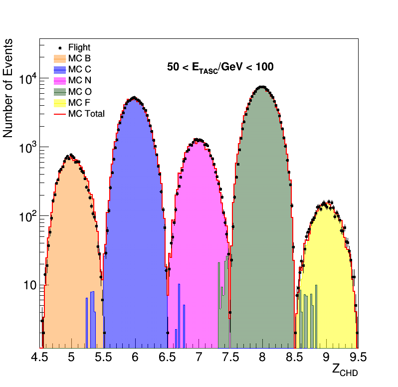
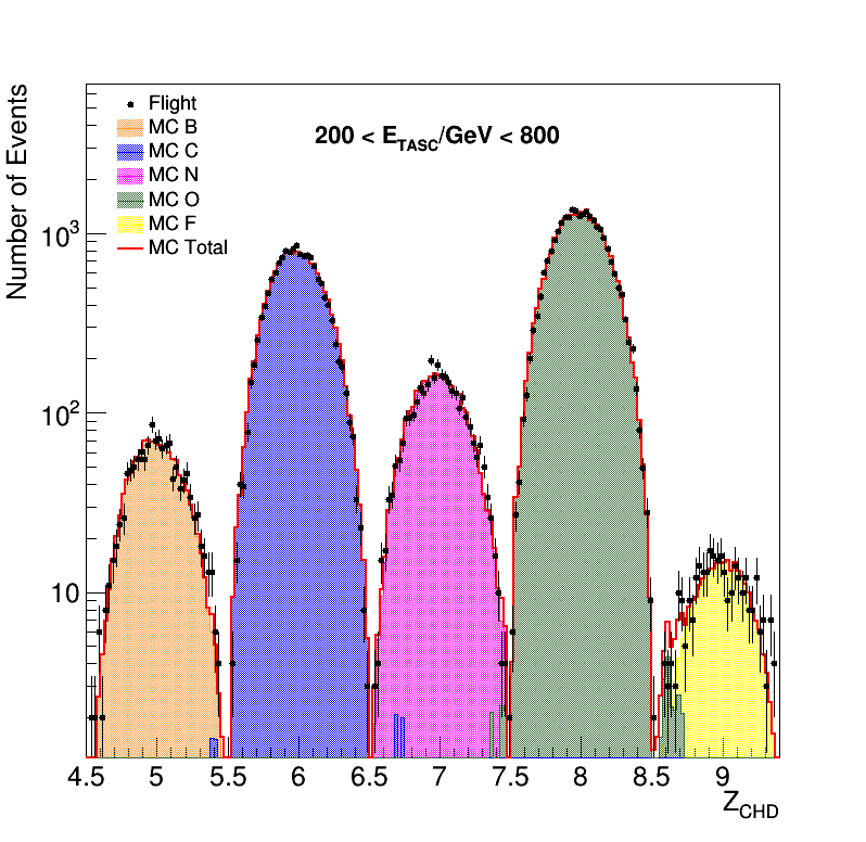
Figure S1: Charge distributions from the combined CHD layers in the elemental region between B and F. Events are selected with (a) $50<E_{\rm TASC}<100$ GeV and (b) $200<E_{\rm TASC}<800$ GeV and a measured charge in IMC consistent with $Z_{\rm CHD}$. FD (black dots) are compared to MC samples. The distributions shown in these plots are only representative of the charge resolution while the relative elemental abundances are not meaningful, because of the different trigger efficiency for different nuclear species (Fig. S7) and different intervals of primary energy per nucleon selected.

The identification of the particle charge $Z$ is based on the measurements of the ionization deposits in CHD and IMC. The particle trajectory is used to identify the CHD paddles and IMC fibers traversed by the primary particle and to determine the path length correction to be applied to the signals to extract the $dE/dx$ samples. Three independent $dE/dx$ measurements are obtained, one for each CHD layer and the third by averaging the samples (at most eight) along the track in the top half of IMC. Calibration curves of $dE/dx$ are built by fitting FD subsets for each nuclear species to a function of $Z^{2}$ by using a ”halo” model Marrocchesi et al. (2011). These curves are then used to reconstruct three charge values ($Z_{\rm CHDX}$, $Z_{\rm CHDY}$, $Z_{\rm IMC}$) from the measured $dE/dx$ on an event-by-event basis Maestro (2019). For high-energy showers, the charge peaks are corrected for the systematical shift to higher values (up to 0.15 $e$) with respect to the nominal charge positions, due to the large amount of shower particle tracks backscattered from TASC whose signals add up to the primary particle ionization signal. A charge distribution obtained by averaging $Z_{\rm CHDX}$ and $Z_{\rm CHDY}$ is shown in Fig. S1 of the SM PRL . The charge resolution $\sigma_{Z}$ is $\sim 0.15\,e$ (charge unit) for CHD and $\sim 0.24\,e$ for IMC, respectively, in the elemental range from B to O.

The shower energy $E_{\rm TASC}$ of each event is calculated as the sum of the energy deposits of all the TASC channels, after stitching the adjacent gain ranges of each PD/APD. The energy response of TASC was studied in a beam test carried out at CERN-SPS in 2015 with accelerated ion fragments of 13, 19 and 150 GeV/c momentum per nucleon  Akaike (2015). The MC simulations were tuned using the beam test results as described in the Energy measurement section of the SM PRL .

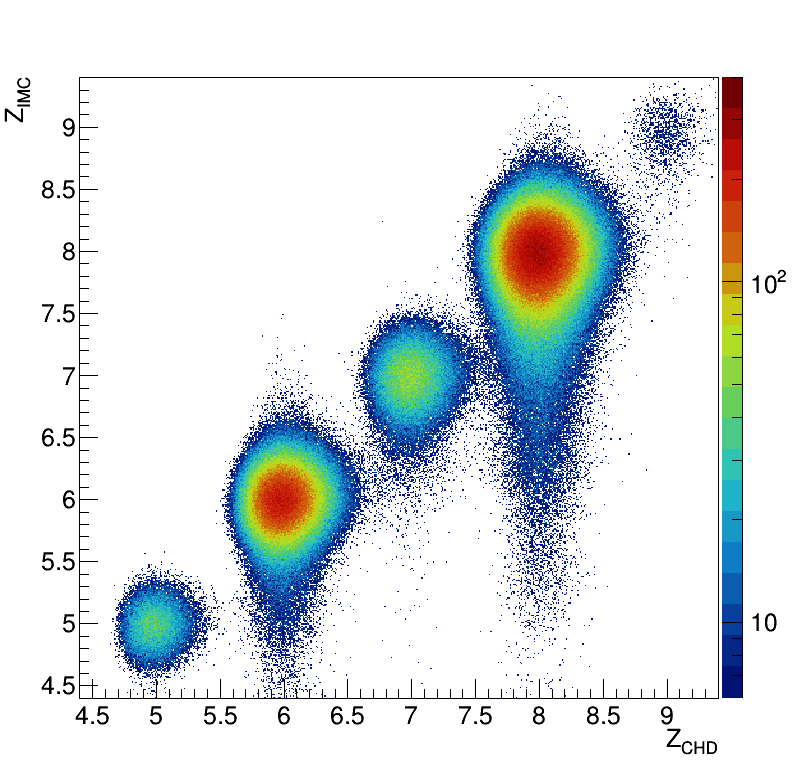
Figure S2: Crossplot of IMC versus CHD reconstructed charges in the elemental range between B and F. Events with C and O nuclei undergoing a charge-changing nuclear interaction upstream the IMC are clearly visible in the tail of their drop-shaped distributions extending to lower $Z_{IMC}$ values. These events are removed in the analysis by requiring the consistency, within 30%, between the mean values of $dE/dx$ measurements in the first four layers in each IMC view and then by applying a window cut to $Z_{\rm IMC}$ of half-width 2$\sigma_{Z}$ centered around the nominal charge values.

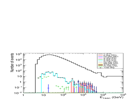
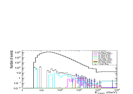
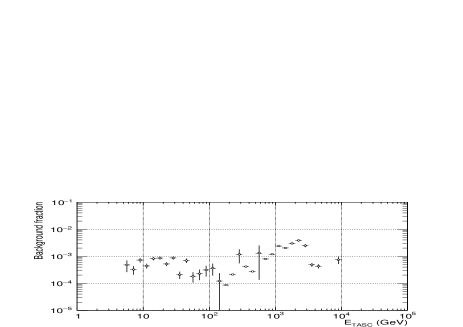
Figure S3: Distributions of $E_{\rm TASC}$ for selected carbon (a) and oxygen (b) events in FD (black line) and estimated contamination from different nuclei. The total background (open black dots) fraction as a function of $E_{\rm TASC}$ is shown for (c) carbon and (d) oxygen. Contamination of each nuclear species with $Z>4$ is estimated by rescaling its $E_{TASC}$ distribution measured in FD by the ratio, estimated with MC simulations, of its reconstruction efficiency to the probability of being misidentified as C or O. Background due to proton and helium is computed by normalizing their $E_{TASC}$ distributions from MC to the number of events expected from previous flux measurements.

Carbon and oxygen candidates are identified among events selected by the onboard HE shower trigger, based on the coincidence of the summed signals of the last two IMC layers in each view and the top TASC layer (TASCX1). Consistency between MC and FD for triggered events is obtained by an offline trigger with higher thresholds (50 and 100 times a minimum ionizing particle (MIP) signal for IMC and TASC, respectively) than the onboard trigger removing possible effects due to residual non-uniformity of the detector gain.
In order to reject possible events triggered by particles entering the TASC from lateral sides or with significant lateral leakage, the energy deposits in the first TASC layer (TASCX1) and in all the lateral bars are required to be less than 40% of $E_{\rm TASC}$. Late-interacting events in the bottom half of TASC are rejected by requiring that the energy deposit in the last layer is $<0.4\times E_{\rm TASC}$, and the layer, where the longitudinal shower development reaches 20% of $E_{\rm TASC}$, occurs in the upper half of TASC.
Events with one well-fitted track crossing the whole detector from CHD top to the TASC bottom layer and at least 2 cm away from the edges in TASCX1 are then selected. The fiducial geometrical factor for this category of events is $S\Omega\sim$510 cm²sr, corresponding to about 50% of the total CALET acceptance.
Carbon and oxygen candidates are selected by applying window cuts, centered on the nominal charge values ($Z=6,8$), of half-width $0.4\,e$ for $Z_{CHDX}$ and $Z_{CHDY}$, and $2\sigma_{Z}$ for $Z_{IMC}$, respectively. Particles undergoing a charge-changing nuclear interaction in the upper part of the instrument (Fig. S2 of the SM PRL ) are removed by the three combined charge selections and by requiring the consistency, within 30%, between the mean values of $dE/dx$ measurements in the first four layers in each IMC view.
Distributions of $E_{\rm TASC}$ for C and O selected candidates are shown in Fig. S3 of SM PRL , corresponding to 6.154$\times 10^{5}$ C and 1.047$\times 10^{6}$ O events, respectively. In order to take into account the relatively limited energy resolution (Fig. S4 of the SM PRL ) energy unfolding is necessary to correct for bin-to-bin migration effects. In this analysis, we used the Bayesian approach D’Agostini (1995) implemented in the RooUnfold package Adye (2011) in ROOT Brun and Rademarkers (1997). Each element of the response matrix represents the probability that primary nuclei in a certain energy interval of the CR spectrum produce an energy deposit in a given bin of $E_{\rm TASC}$. The response matrix (Fig. S5 of the SM PRL ) is derived using MC simulation after applying the same selection procedure as for FD.
The energy spectrum is obtained from the unfolded energy distribution as follows:

$$\Phi(E)=\frac{N(E)}{\Delta E\;\varepsilon(E)\;S\Omega\;T}$$ (1)

$$N(E)=U\left[N_{obs}(E_{\rm TASC})-N_{bg}(E_{\rm TASC})\right]$$ (2)

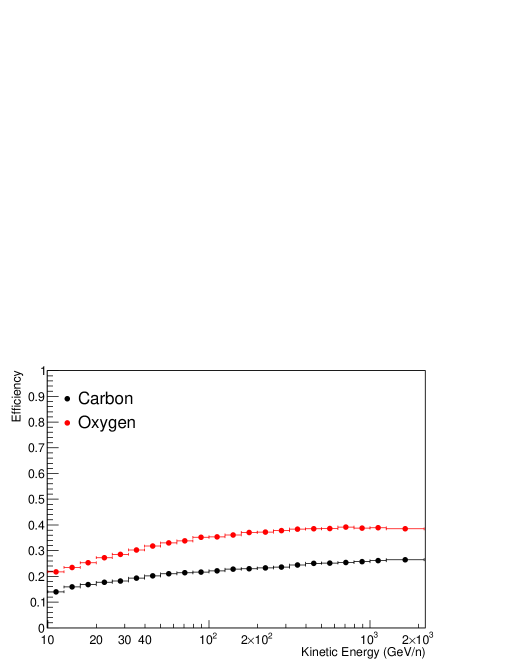
Figure S6: Total selection efficiency for C (black dots) and O (red dots) estimated with MC simulations.

where $\Delta E$ denotes energy bin width, $E$ the particle kinetic energy, calculated as the geometric mean of the lower and upper bounds of the bin, $N(E)$ is the bin content in the unfolded distribution, $\varepsilon(E)$ the total selection efficiency (Fig. S6 of the SM PRL ), $U()$ the unfolding procedure, $N_{obs}(E_{\rm TASC})$ the bin content of observed energy distribution (including background), $N_{bg}(E_{\rm TASC})$ the bin content of background events in the observed energy distribution. Background contamination from different nuclear species misidentified as C or O is shown in Fig. S3 of the SM PRL . A contamination fraction $N_{bg}/N_{obs}<0.1\%$ is found in all energy bins with $E_{\rm TASC}<10^{3}$ GeV, and between 0.1% and 1% for $E_{TASC}>10^{3}$ GeV.

IV Systematic Uncertainties

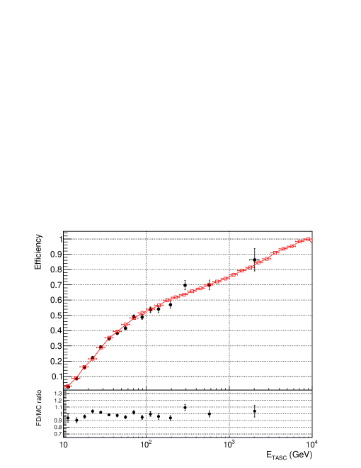
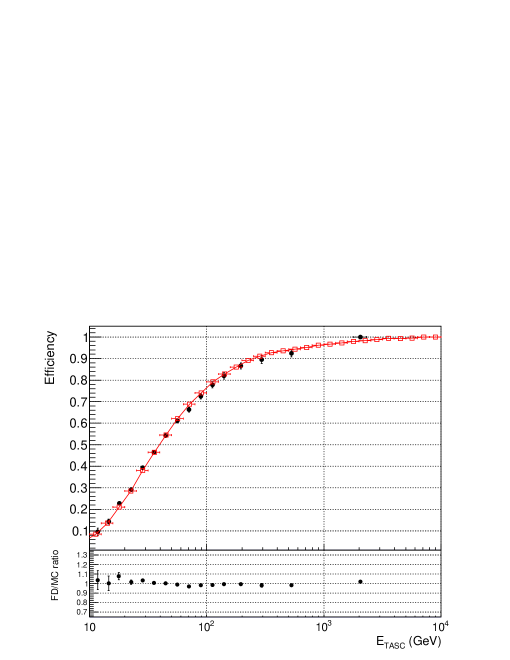
Figure S7: HE trigger efficiency as a function of the deposited energy in TASC for C (a) and O (b) as derived from flight data (FD) (black dots) and Monte Carlo (MC) (red rectangles). The FD to MC efficiency ratio is shown in the lower canvas. The HE trigger efficiency was measured directly from the data by using dedicated runs where in addition to HE, a low-energy (LE) trigger was active. The trigger logic is the same for both trigger (i.e. coincidence of the pulse heights of the last two pairs of IMC layers and the top TASC layer) but lower discriminator thresholds are set for the input signals in case of LE trigger, allowing to trigger also penetrating nuclei with $Z>2$. The ratio of the number of events counted by both triggers to those registered by the LE trigger only is an estimate of the HE trigger efficiency in each bin of deposited energy. To compare with simulations, we apply exactly the same method to MC samples, where both trigger modes are modeled.

In this analysis, dominant sources of systematic uncertainties include trigger efficiency, energy response, event selection, unfolding procedure, MC model.
HE trigger efficiency as a function of $E_{\rm TASC}$ was inferred from the data taken with a minimum bias trigger. HE efficiency curves for C and O are consistent with predictions from MC simulations, as shown in Fig. S7 of the SM PRL . In order to study the flux stability against offline trigger efficiency, the threshold applied to TASCX1 signal was scanned between 100 and 150 MIP signal. The corresponding systematic errors range between -4.2% (-3.1%) and 3.7% (7.3%) for C (O) depending on the energy bin.
The systematic error related to charge identification was studied by varying the width of the window cuts between 0.35 $e$ and 0.45 $e$ for CHD and between 1.75 $\sigma_{Z}$ and 2.2 $\sigma_{Z}$ for IMC. That results in a flux variation depending on the energy bin, which is less than 1% below 250 $\text{GeV}/n$ and few percent above. The ratio of events selected by IMC charge cut to the ones selected with CHD in different $E_{\rm TASC}$ intervals turned out to be consistent in FD and MC.
Possible inaccuracy of track reconstruction could affect the determination of the geometrical acceptance. The contamination due to off-acceptance events which are mis-reconstructed in the fiducial acceptance was estimated with MC to be $\sim 1\%$ at 10 GeV$/n$ and decrease to less than $0.1\%$ above 60 GeV$/n$. To investigate the uncertainty in the definition of the acceptance, restricted acceptance (up to 20% of nominal one) regions were also studied. The corresponding fluxes are consistent within statistical fluctuations.
A different tracking procedure, described in Ref. Akaike (2019), was also used to study possible systematic uncertainties in tracking efficiency. Results are consistent with those obtained with the Kalman filter algorithm, hence we consider negligible this source of systematic error.
The uncertainty in the energy scale is $\pm 2$% and depends on the accuracy of the beam test calibration. It causes a rigid shift of the measured energies, affecting the absolute normalization of the C and O spectra by ${}^{+2.6\%}_{-2.8\%}$, but not their shape. As the beam test model was not identical to the instrument now in orbit, the difference in the spectrum obtained with either configuration was modeled and included in the systematic error.
Other energy-independent systematic uncertainties affecting the normalization include live time (3.4%, as explained in the SM of Ref. Adriani et al. (2017)) and long-term stability of the charge measurements ($<0.4\%$).
The uncertainties due to the unfolding procedure were evaluated by using different response matrices, computed by varying the spectral index (between -2.9 and -2.5) of the generation spectrum of MC simulations, and the Singular Value Deconvolution method, instead of the Bayesian approach, in RooUnfold software Adye (2011).
Since it is not possible to validate MC simulations with beam test data in the high-energy region, a comparison between different MC models, i.e. EPICS and FLUKA, was performed. We found that the total selection efficiencies for C and O determined with the two models are in agreement within $<1.5\%$ over the whole energy range, but the energy response matrices differ significantly in the low and high energy regions. The resulting fluxes show maximum discrepancies of 9% (7.8%) and 9.2% (12.2%), respectively, in the first and last energy bin for C (O), while they are consistent within 6.6% (6.2%) elsewhere. This is the dominant source of systematic uncertainties.
Materials traversed by nuclei in IMC are mainly composed of carbon, aluminum and tungsten. Possible uncertainties in the inelastic cross sections in simulations or discrepancies in the material description might affect the flux normalization. We have checked that hadronic interactions are well simulated in the detector, by measuring the survival probabilities of C and O nuclei at different depths in IMC, as described in the SM PRL . The survival probabilities are in agreement with MC prediction within $<1\%$ (Fig. S8 of the SM PRL ).
Background contamination from different nuclear species estimated with FLUKA and EPICS simulations differ by less than $1\%$.
The energy dependence of all the systematic uncertainties for C and O is shown in Fig. S9 of the SM PRL . The total systematic error is computed as the sum in quadrature of all the sources of systematics in each energy bin.

V Results

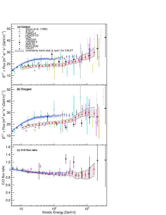
Figure S10: CALET (a) carbon and (b) oxygen flux (multiplied by $E^{2.7}$) and (c) ratio of carbon to oxygen fluxes, as a function of kinetic energy $E$. Error bars of CALET data (red) represent the statistical uncertainty only, while the gray band indicates the quadratic sum of statistical and systematic errors. Also plotted are other direct measurements Engelmann et al. (1990); Müller et al. (1991); Panov et al. (2009); Ave et al. (2008); Aguilar et al. (2017); Adriani et al. (2014); Ahn et al. (2009); Atkin et al. (2017); Simon et al. (1980).

The energy spectra of carbon and oxygen and their flux ratio measured with CALET in an energy range from 10 GeV$/n$ to 2.2 TeV$/n$ are shown in Fig. S10, where current uncertainties that include statistical and systematic errors are bounded within a gray band. CALET spectra are compared with results from space-based Engelmann et al. (1990); Müller et al. (1991); Adriani et al. (2014); Aguilar et al. (2017); Atkin et al. (2017) and balloon-borne Simon et al. (1980); Panov et al. (2009); Ave et al. (2008); Ahn et al. (2009) experiments. The measured C and O fluxes and flux ratio with statistical and systematic errors are tabulated in Tables I, II and III of the SM PRL .

Figure 1: CALET (a) carbon and (b) oxygen flux (multiplied by $E^{2.7}$) and (c) ratio of carbon to oxygen fluxes, as a function of kinetic energy $E$. Error bars of CALET data (red) represent the statistical uncertainty only, while the gray band indicates the quadratic sum of statistical and systematic errors. Also plotted are other direct measurements Engelmann et al. (1990); Müller et al. (1991); Panov et al. (2009); Ave et al. (2008); Aguilar et al. (2017); Adriani et al. (2014); Ahn et al. (2009); Atkin et al. (2017); Simon et al. (1980). An enlarged version of the figure is available as Fig. S10 in the SM PRL .

.

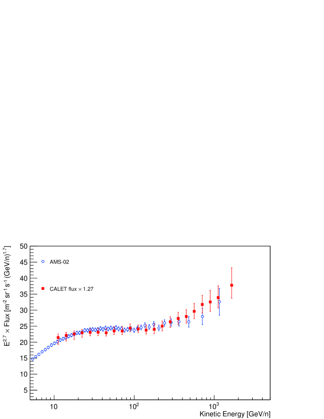
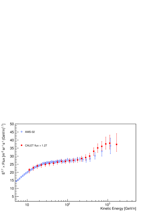
Figure S11: (a) Carbon and (b) oxygen fluxes measured by CALET (red points) are multiplied by 1.27 for comparison with AMS-02 results Aguilar et al. (2017). Error bars of CALET data represent the quadratic sum of statistical and systematic uncertainties. The factor (1.27$\pm$0.03) is obtained by a simultaneous minimization of the sum of squared residuals between CALET and AMS data points for C and O.

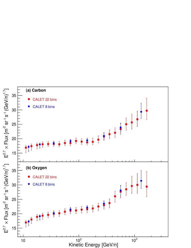
Figure S14: CALET carbon (a) and oxygen (b) spectra derived with two different energy binnings. In the reference spectra (red squares) the energy range from 10 GeV$/n$ to 2.2 TeV$/n$ is divided into 22 bins (Tables I and II); all bins are chosen to have relative width commensurate with the TASC energy resolution $\sigma_{E}$, with the exception of the last bin whose width is $2\times\sigma_{E}$. To study possible binning related effects in the spectra, C and O fluxes are also derived by dividing the energy range into 8 bins (blue dots), with relative bin width $\sim 2.5\times\sigma_{E}$, but the last bin whose width is $3.5\times\sigma_{E}$. The wide-bin spectra have the same shape as the original ones. The flux differences are well within the error bars, representing the quadratic sum of statistical and systematic uncertainties.

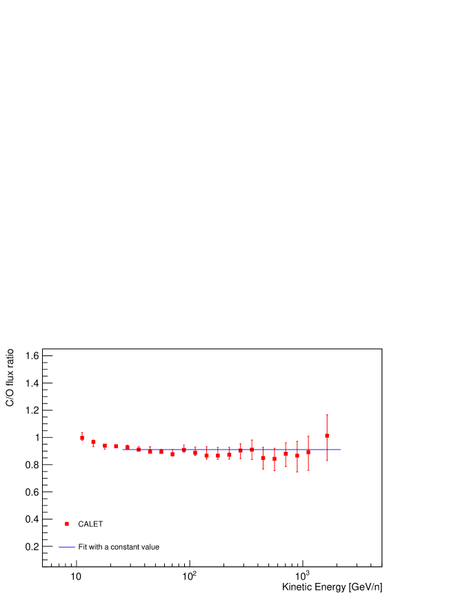
Figure S15: The carbon to oxygen flux ratio as a function of kinetic energy per nucleon is fitted to a constant function (blue line). Error bars of CALET data points represent the sum in quadrature of statistical and systematic uncertainties. Above 25 GeV$/n$ the C/O ratio is described by a constant value of $0.911\pm 0.006$ with $\chi^{2}/$d.o.f. = 8.3/17.

Our spectra are consistent with PAMELA  Adriani et al. (2014) and most previous experiments Engelmann et al. (1990); Müller et al. (1991); Panov et al. (2009); Ave et al. (2008); Ahn et al. (2009), but the absolute normalization is in tension with AMS-02 Aguilar et al. (2017). However we notice that C/O ratio (Fig. S10 (c)) is consistent with the one measured by AMS-02. In Fig. S11 of the SM PRL , it is shown that CALET and AMS-02 C and O spectra have very similar shapes but they differ in the absolute normalization, which is lower for CALET by about 27% for both C and O.
Figure 2 shows the fits to CALET carbon and oxygen data with a double power-law function (DPL, Eq. S1 in SM PRL ) above 25 GeV$/n$. A single power-law function (SPL, Eq. S2 in SM PRL )) fitted to data in the energy range [25, 200] GeV$/n$ and extrapolated above 200 GeV$/n$ is also shown for comparison. The effect of systematic uncertainties in the measurement of the energy spectrum is modeled in the $\chi^{2}$ minimization function with a set of 6 nuisance parameters as explained in detail in the SM PRL . The DPL fit to the C spectrum yields a spectral index $\gamma=-2.663\pm 0.014$ at energies below the transition region $E_{0}=(215\pm 54)$ GeV$/n$ and a spectral index increase $\Delta\gamma=0.166\pm 0.042$ above, with $\chi^{2}/$d.o.f. = 9.0/8. For oxygen, the fit yields $\gamma=-2.637\pm 0.009$, $E_{0}=(264\pm 53)$ GeV$/n$, $\Delta\gamma=0.158\pm 0.053$, with $\chi^{2}/$d.o.f. = 3.0/8. SPL fits to CALET carbon and oxygen data above 25 GeV$/n$ are shown in Figs. S12 and S13 of the SM PRL . They give $\gamma=-2.626\pm 0.010$ with $\chi^{2}/$d.o.f. = 27.5/10 for C, and $\gamma=-2.622\pm 0.008$ with $\chi^{2}/$d.o.f. = 15.9/10 for O, respectively. A frequentist test statistic $\Delta\chi^{2}$ is computed from the difference in $\chi^{2}$ between the fits with SPL and DPL functions. For carbon (oxygen), $\Delta\chi^{2}=18.5$ (12.9) with 2 d.o.f. (i.e. the number of additional free parameters in DPL fit with respect to SPL fit) implies that the significance of the hardening of the C (O) spectrum exceeds the 3$\sigma$ level. We also checked that the spectral hardening is not an artifact of the energy binning and unfolding, by increasing the bin width by a factor 2.5 as shown in Fig. S14 of the SM PRL . The resulting flux difference is negligible when compared with our estimated systematic uncertainties.
In order to study the energy dependence of the spectral index in a model independent way, the spectral index $\gamma$ is calculated by a fit of $d[\log(\Phi)]/d[\log(E)]$ in energy windows centered in each bin and including the neighbor $\pm$3 bins. The results in Fig. 3 show that carbon and oxygen fluxes harden in a similar way above a few hundred GeV$/n$. The carbon to oxygen flux ratio is well fitted to a constant value of $0.911\pm 0.006$ above 25 GeV$/n$ (Fig. S15 of the SM PRL ), indicating that the two fluxes have the same energy dependence.

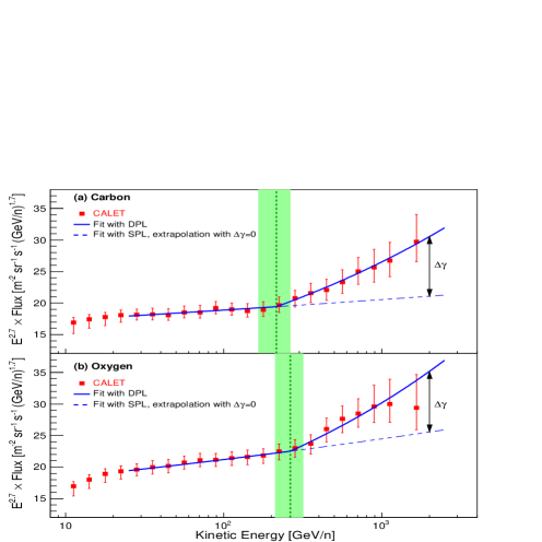
Figure 2: Fit of the CALET (a) C and (b) O energy spectra with a DPL function (blue line) in the energy range [25, 2000] GeV$/n$. The flux is multiplied by $E^{2.7}$ where $E$ is the kinetic energy per nucleon. Error bars of CALET data points represent the sum in quadrature of statistical and systematic uncertainties. The dashed blue lines represent the extrapolation of a SPL function fitted to data in the energy range [25, 200] GeV$/n$. $\Delta\gamma$ is the change of the spectral index above the transition energy $E_{0}$, represented by the vertical green dashed line. The error interval for $E_{0}$ from the DPL fit is shown by the green band.

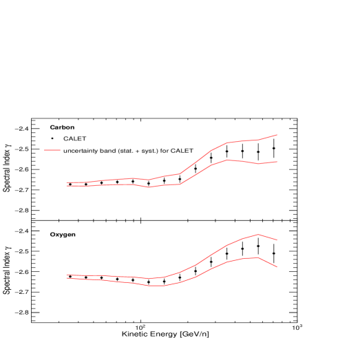
Figure 3: Energy dependence of the spectral index calculated within a sliding energy window for CALET (a) C and (b) O data. The spectral index is determined for each bin by fitting the data using $\pm$3 bins. Red curves indicate the uncertainty range including systematic errors.

VI Conclusion

With a calorimetric apparatus in low Earth orbit, CALET has measured the energy spectra of carbon and oxygen nuclei in CR and their flux ratio from 10 GeV$/n$ to 2.2 TeV$/n$. Our observations allow to exclude a single power law spectrum for C and O by more than $3\sigma$; they show a spectral index increase $\Delta\gamma=0.166\pm 0.042$ for C and $\Delta\gamma=0.158\pm 0.053$ for O above 200 GeV$/n$, and the same energy dependence for C and O fluxes with a constant C/O flux ratio $0.911\pm 0.006$ above 25 GeV$/n$. These results are consistent with the ones reported by AMS-02. However the absolute normalization of our data is significantly lower than AMS-02, but in agreement with previous experiments. Improved statistics and refinement of the analysis with additional data collected during the lifetime of the mission will allow to extend the measurements at higher energies and improve the spectral analysis, contributing to a better understanding of the origin of the spectral hardening.

VII Acknowledgments

Supplemental material concerning “Direct Measurement of the Cosmic-Ray Carbon and Oxygen spectra from 10 GeV$/n$ to 2.2 TeV$/n$ with the Calorimetric Electron Telescope on the International Space Station”

VIII Energy measurement

Differently from the case of electrons, the energy released in TASC by interacting CR nuclei is only a fraction of the primary particle energy, the electromagnetic component of the hadronic cascades, originating from the decays of $\pi^{0}$ secondaries produced in the showers. Though a significant part of the hadronic cascade energy leaks out of the calorimeter because of its limited thickness (1.3 $\lambda_{I}$), the energy deposited in the TASC by the electromagnetic shower core scales linearly with the incident particle energy, albeit with large event-to-event fluctuations. As a result, the energy resolution is poor by the standards of total containment hadron calorimetry in experiments at accelerators. Nevertheless, it is sufficient to reconstruct the steep energy spectra of CR nuclei with a nearly energy independent resolution.
The TASC response to nuclei was studied at CERN SPS in 2015 using a beam of accelerated ion fragments with $A/Z=2$ and kinetic energy of 13, 19 and 150 GeV$/n$ Akaike (2015). In Fig. S4a, the $E_{\rm TASC}$ distributions for C nuclei at 150 GeV/n is shown as an example. C nuclei in the beam are selected with CHD and the HE trigger is applied. The resulting distribution looks nearly gaussian, the energy released in the TASC is $\sim$20% of the particle energy and the resolution $\sigma_{E}$ is close to 30%. The mean energy deposited in TASC by different nuclear species in the beam (selected with CHD) is plotted as a function of the kinetic energy per particle in Fig. S4b. The energy response of TASC is linear up to the maximum available particle energy of 6 TeV (obtained with a primary beam of ⁴⁰Ar nuclei).
The energy response derived from MC simulations was tuned using the beam test results. Correction factors are 6.7% for $E_{\rm TASC}<45$ GeV and 3.5% for $E_{\rm TASC}>350$ GeV, respectively, while a simple linear interpolation is used to determine the correction factor for intermediate energies.
For flux measurement, energy unfolding is applied to correct $E_{\rm TASC}$ distributions of selected C and O candidates for significant bin-to-bin migration effects (due to the limited energy resolution) and infer the primary particle energy. In this analysis, we apply the iterative unfolding method based on the Bayes’ theorem D’Agostini (1995) implemented in the RooUnfold package Adye (2011); Brun and Rademarkers (1997). The response matrix is derived using MC simulations of the CALET flight model after applying the same selection as for FD and used in the unfolding procedure (Fig. S5). Each element of the matrix represents the probability that primary nuclei in a certain energy interval of the CR spectrum produce an energy deposit in a given $E_{\rm TASC}$ bin.

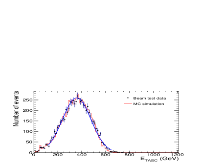
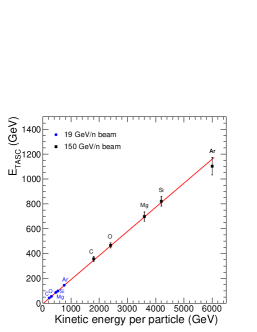
Figure S4: (a) Energy deposited in TASC by a beam of accelerated C nuclei of fixed energy 150 GeV/n at CERN-SPS Akaike (2015). The data are fitted to a gaussian (blue line); the mean value is 20% of the kinetic beam particle energy, and the energy resolution (defined as the standard deviation to mean ratio) is $\sim$30%. (b) Energy linearity of TASC as measured at CERN SPS with beams of 19 (blue dots) and 150 (black squares) GeV$/n$ ion fragments with $A/Z=2$. The red line represents a linear fit to the data. The fitted slope is $0.194\pm 0.005$, indicating that on average $\sim$20% of the particle energy is deposited in TASC.

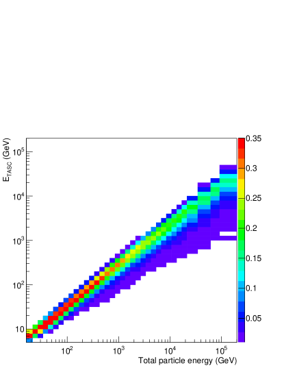
Figure S5: Response matrix for oxygen derived from MC simulations of the CALET flight model by applying the same selection as for FD. The color scale is associated to the probability that nuclei of a given energy produce showers in different intervals of $E_{\rm TASC}$.

IX Survival probabilities

In order to check that hadronic interactions in the detector are well simulated, we have measured the survival probabilities of C and O nuclei at different depths in IMC and compared with the ones expected from MC simulations. For each HE-triggered event, selected as C or O by means of CHD only, several measurements of the charge are obtained by dE/dx samples along the particle track in pairs of adjacent scintillating-fiber (SciFi) layers. The coupled SciFi layers are spaced by about 2.3 cm and interleaved with W plates (except for the first pair), aluminum honeycomb panels and CFRP (carbon fiber reinforced polymer) supporting structures. From the charge distribution of each pair of Scifi layers, the number of events that did not interact in the material upstream the fibers can be estimated by selecting the nuclei with a charge value consistent with the one measured in CHD. The reduction in the number of not-interacted events, normalized to the ones selected in CHD, allows to measure the survival probability as a function of the material thickness traversed by the particle in the IMC, as shown in Fig. S8. In MC data, the survival probabilities can be calculated by using the true information on the point where the first hadronic interaction occurs in the detector. The survival probabilities measured in FD are in good agreement (within $<1\%$) with MC predictions, as shown in the bottom panels of Fig. S8.

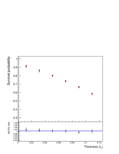
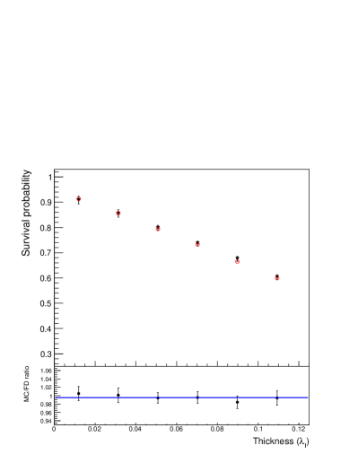
Figure S8: Survival probability as a function of the material thickness traversed by the particles in IMC as derived from FD (black triangles) and MC (red circles) for carbon (a) and oxygen (b) (upper panels). The survival probabilities are calculated in FD by dividing the number of events selected as C (O) in the first six pairs of SciFi layers in IMC by the number of C (O) events selected with CHD. The material thickness is expressed in units of proton interaction length $\lambda_{I}$ and it is measured from the bottom of CHD. The coupled SciFi layers are preceded by 0.2 $X_{0}$-thick W plates (except the first pair), Al honeycomb panels and CFRP supporting structures. In bottom panels, the blue dotted line represents a constant value fitted to the ratio between MC and FD survival probabilities. The fitted value is $0.997\pm 0.008$ ($1.006\pm 0.006$) for O (C).

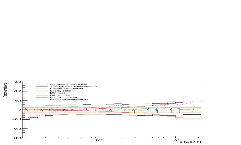
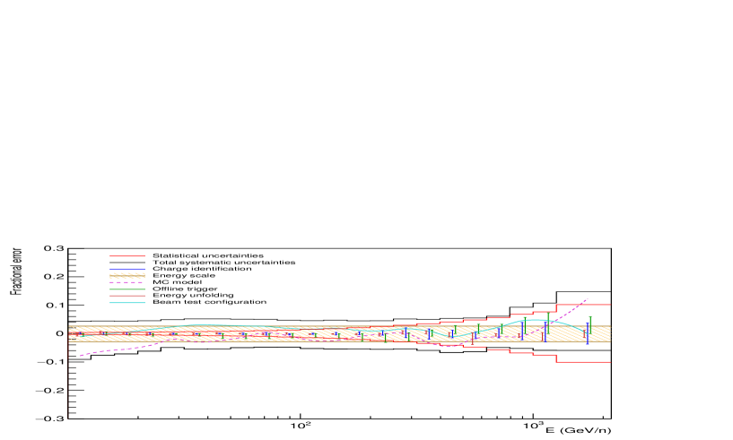
Figure S9: Energy (per nucleon in GeV) dependence of systematic uncertainties (relative errors) for C (a) and O (b). The band defined by the red lines represents the statistical error in each energy bin. The band within the black lines shows the sum in quadrature of all the sources of systematics. A detailed breakdown of systematic errors, stemming from charge identification, offline trigger, MC model, energy scale correction, energy unfolding and beam test configuration, is shown.

X Spectral fit method

We have tested two models for the C and O energy spectra: a double power-law (DPL) in energy

$$\Phi(E)=\begin{cases}C\left(\frac{E}{\text{GeV}}\right)^{\gamma}&E\leq E_{0}\\ C\left(\frac{E}{\text{GeV}}\right)^{\gamma}\left(\frac{E}{E_{0}}\right)^{\Delta\gamma}&E>E_{0}\end{cases}$$ (S1)

and a single power-law (SPL)

$$\Phi(E)=C\,\left(\frac{E}{\text{GeV}}\right)^{\gamma}$$ (S2)

where $C$ is a normalization factor, $\gamma$ the spectral index, and $\Delta\gamma$ the spectral index change above the transition energy $E_{0}$. We have fitted the data using a chi-square minimization. The effect of systematic uncertainties in the measurement of the energy spectrum is modeled introducing in the $\chi^{2}$ function a set of nuisance parameters.
The $\chi^{2}$ function is defined as

$$\chi^{2}=\sum_{i=4}^{N}\left[\frac{\Phi_{i}+S(E_{i},\bm{\beta})\sigma_{i}^{sys}-\Phi(E_{i},\bf{p})}{\sigma^{stat}_{i}}\right]^{2}+\sum_{j=1}^{N_{np}}\beta_{i}^{2}$$ (S3)

where $\Phi_{i}$, $\sigma_{i}^{stat}$, $\sigma_{i}^{sys}$, $E_{i}$ are the measured flux, the statistical and systematic errors, and the energy of the $i$-th bin (geometric mean of bin edges), respectively; $N=22$ is the number of data points and the fit starts from the fourth point. The elements of the vector $\bf{p}$ are the free parameters of the model function $\Phi$ used in the fit: ${\bf p}=\{C,\gamma,\Delta\gamma,E_{0}\}$ for Eq. S1, and ${\bf p}=\{C,\gamma\}$ for Eq. S2.
$\bm{\beta}$ is a set of independent nuisance parameters $\beta_{j}$ with $j=1,...,N_{np}$ introduced to properly account for systematic uncertainties in the fit. The energy range to be fitted (from 25 to 2200 GeV$/n$) is logarithmically divided into $N_{np}$ intervals. According to the energy dependence of the systematic fractional errors (Fig. S9), we chose $N_{np}=6$; therefore the width of each interval covers three consecutive energy bins of the spectrum. A nuisance parameter $\beta_{j}$ is assigned to each interval. In the fit, a gaussian constraint (the last term in Eq. S3) is applied to each parameter $\beta_{j}$, with zero mean and standard deviation equal to 1. In the $\chi^{2}$ function, the systematic errors $\sigma_{i}^{sys}$ are multiplied by a piece-wise function $S(E_{i},\bm{\beta})$, which assumes the value of $\beta_{j}$ of the corresponding energy interval within which $E_{i}$ falls.
The results of the fits with the two models are shown in Figs. S12 and S13 for C and O spectrum, respectively. We also performed the fits by varying the number of nuisance parameters, with similar results and significance.

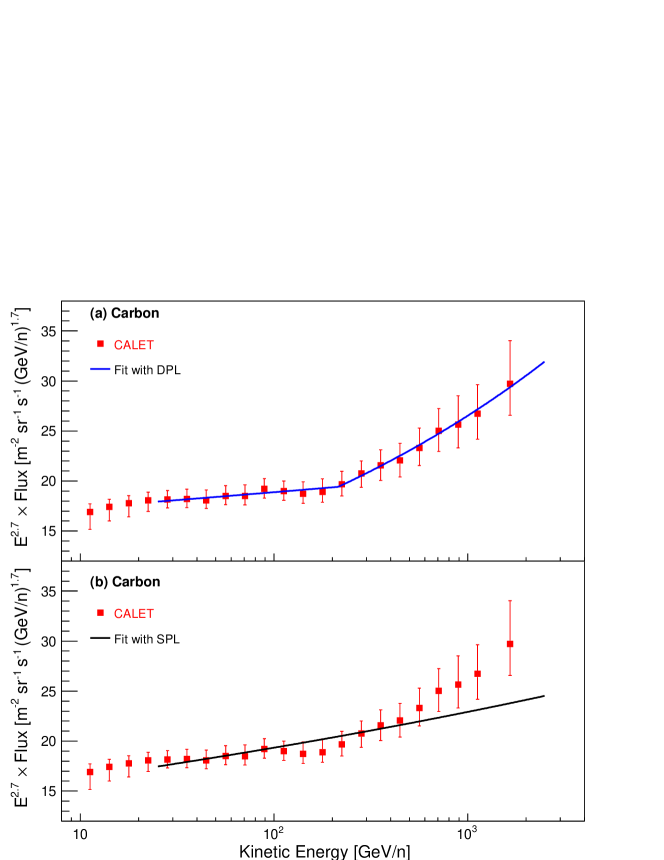
Figure S12: Fit to the carbon energy spectrum with (a) a DPL function (Eq. S1) and (b) a SPL function (Eq. S2), in the energy range [25, 2000] GeV/n. Error bars of CALET data points represent the sum in quadrature of statistical and systematic uncertainties. The DPL fit yields $\gamma=-2.663\pm 0.014$, $E_{0}=(215\pm 54)$ GeV$/n$, $\Delta\gamma=0.166\pm 0.042$, with $\chi^{2}/$d.o.f. = 9.0/8. The SPL fit yields $\gamma=-2.626\pm 0.010$ with $\chi^{2}/$d.o.f. = 27.5/10. The difference $\Delta\chi^{2}=18.5$ between the fits with the two models, with two additional free parameters in DPL fit with respect to SPL fit, allows to exclude the single power law hypothesis at the 3.9$\sigma$ level.

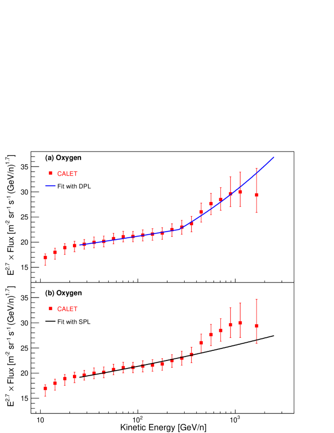
Figure S13: Fit to the oxygen energy spectrum with (a) a DPL function (Eq. S1) and (b) a SPL function (Eq. S2), in the energy range [25, 2000] GeV$/n$. Error bars of CALET data points represent the sum in quadrature of statistical and systematic uncertainties. The DPL fit yields $\gamma=-2.637\pm 0.009$, $E_{0}=(264\pm 53)$ GeV$/n$, $\Delta\gamma=0.158\pm 0.053$, with $\chi^{2}/$d.o.f. = 3.0/8. The SPL fit yields $\gamma=-2.622\pm 0.008$ with $\chi^{2}/$d.o.f. = 15.9/10. The difference $\Delta\chi^{2}=12.9$ between the fits with the two models, with two additional free parameters in DPL fit with respect to SPL fit, allows to exclude the single power law hypothesis at the 3.2$\sigma$ level.

Table 1: Table of CALET carbon spectrum. The first, second and third error in the flux represents the statistical uncertainties, systematic uncertainties in normalization, and energy dependent systematic uncertainties, respectively.

Energy Bin [GeV$/n$]	Flux [m-2sr-1s-1(GeV$/n$)-1]
10.0–12.6	$(2.471\,\pm 0.008\,_{-0.110}^{+0.106}\,{}_{-0.226}^{+0.058})\times 10^{-2}$
12.6–15.8	$(1.368\,\pm 0.005\,_{-0.061}^{+0.059}\,{}_{-0.092}^{+0.009})\times 10^{-2}$
15.8–20.0	$(7.492\,\pm 0.032\,_{-0.332}^{+0.321}\,{}_{-0.461}^{+0.047})\times 10^{-3}$
20.0–25.1	$(4.092\,\pm 0.020\,_{-0.182}^{+0.175}\,{}_{-0.172}^{+0.051})\times 10^{-3}$
25.1–31.6	$(2.208\,\pm 0.013\,_{-0.098}^{+0.095}\,{}_{-0.028}^{+0.051})\times 10^{-3}$
31.6–39.8	$(1.189\,\pm 0.008\,_{-0.053}^{+0.051}\,{}_{-0.019}^{+0.038})\times 10^{-3}$
39.8–50.1	$(6.341\,\pm 0.049\,_{-0.281}^{+0.271}\,{}_{-0.058}^{+0.236})\times 10^{-4}$
50.1–63.1	$(3.487\,\pm 0.031\,_{-0.155}^{+0.149}\,{}_{-0.048}^{+0.122})\times 10^{-4}$
63.1–79.4	$(1.871\,\pm 0.020\,_{-0.083}^{+0.080}\,{}_{-0.022}^{+0.078})\times 10^{-4}$
79.4–100.0	$(1.044\,\pm 0.013\,_{-0.046}^{+0.045}\,{}_{-0.012}^{+0.031})\times 10^{-4}$
100.0–125.9	$(5.545\,\pm 0.084\,_{-0.246}^{+0.237}\,{}_{-0.071}^{+0.141})\times 10^{-5}$
125.9–158.5	$(2.932\,\pm 0.053\,_{-0.130}^{+0.125}\,{}_{-0.049}^{+0.128})\times 10^{-5}$
158.5–199.5	$(1.590\,\pm 0.034\,_{-0.071}^{+0.068}\,{}_{-0.035}^{+0.082})\times 10^{-5}$
199.5–251.2	$(8.890\,\pm 0.228\,_{-0.394}^{+0.381}\,{}_{-0.264}^{+0.378})\times 10^{-6}$
251.2–316.2	$(5.035\,\pm 0.154\,_{-0.223}^{+0.216}\,{}_{-0.193}^{+0.154})\times 10^{-6}$
316.2–398.1	$(2.812\,\pm 0.100\,_{-0.125}^{+0.120}\,{}_{-0.117}^{+0.127})\times 10^{-6}$
398.1–501.2	$(1.544\,\pm 0.065\,_{-0.068}^{+0.066}\,{}_{-0.067}^{+0.076})\times 10^{-6}$
501.2–631.0	$(8.766\,\pm 0.432\,_{-0.389}^{+0.375}\,{}_{-0.339}^{+0.468})\times 10^{-7}$
631.0–794.3	$(5.053\,\pm 0.292\,_{-0.224}^{+0.216}\,{}_{-0.204}^{+0.264})\times 10^{-7}$
794.3–1000.0	$(2.780\,\pm 0.190\,_{-0.123}^{+0.119}\,{}_{-0.112}^{+0.215})\times 10^{-7}$
1000.0–1258.9	$(1.555\,\pm 0.122\,_{-0.069}^{+0.067}\,{}_{-0.047}^{+0.097})\times 10^{-7}$
1258.9–2166.7	$(6.094\,\pm 0.578\,_{-0.270}^{+0.261}\,{}_{-0.116}^{+0.613})\times 10^{-8}$

Table 2: Table of CALET oxygen spectrum. The first, second and third error in the flux represents the statistical uncertainties, systematic uncertainties in normalization, and energy dependent systematic uncertainties, respectively.

Energy Bin [GeV$/n$]	Flux [m-2sr-1s-1(GeV$/n$)-1]
10.0–12.6	$(2.479\,\pm 0.009\,_{-0.110}^{+0.106}\,{}_{-0.198}^{+0.013})\times 10^{-2}$
12.6–15.8	$(1.414\,\pm 0.005\,_{-0.063}^{+0.061}\,{}_{-0.088}^{+0.016})\times 10^{-2}$
15.8–20.0	$(7.977\,\pm 0.035\,_{-0.354}^{+0.341}\,{}_{-0.450}^{+0.056})\times 10^{-3}$
20.0–25.1	$(4.374\,\pm 0.022\,_{-0.194}^{+0.187}\,{}_{-0.191}^{+0.063})\times 10^{-3}$
25.1–31.6	$(2.381\,\pm 0.014\,_{-0.106}^{+0.102}\,{}_{-0.050}^{+0.056})\times 10^{-3}$
31.6–39.8	$(1.305\,\pm 0.009\,_{-0.058}^{+0.056}\,{}_{-0.041}^{+0.039})\times 10^{-3}$
39.8–50.1	$(7.074\,\pm 0.054\,_{-0.314}^{+0.303}\,{}_{-0.215}^{+0.210})\times 10^{-4}$
50.1–63.1	$(3.901\,\pm 0.035\,_{-0.173}^{+0.167}\,{}_{-0.088}^{+0.106})\times 10^{-4}$
63.1–79.4	$(2.134\,\pm 0.022\,_{-0.095}^{+0.091}\,{}_{-0.041}^{+0.055})\times 10^{-4}$
79.4–100.0	$(1.148\,\pm 0.014\,_{-0.051}^{+0.049}\,{}_{-0.021}^{+0.021})\times 10^{-4}$
100.0–125.9	$(6.250\,\pm 0.092\,_{-0.277}^{+0.267}\,{}_{-0.179}^{+0.097})\times 10^{-5}$
125.9–158.5	$(3.384\,\pm 0.058\,_{-0.150}^{+0.145}\,{}_{-0.106}^{+0.066})\times 10^{-5}$
158.5–199.5	$(1.836\,\pm 0.038\,_{-0.081}^{+0.079}\,{}_{-0.056}^{+0.023})\times 10^{-5}$
199.5–251.2	$(1.017\,\pm 0.025\,_{-0.045}^{+0.044}\,{}_{-0.033}^{+0.015})\times 10^{-5}$
251.2–316.2	$(5.577\,\pm 0.164\,_{-0.247}^{+0.239}\,{}_{-0.170}^{+0.158})\times 10^{-6}$
316.2–398.1	$(3.088\,\pm 0.106\,_{-0.137}^{+0.132}\,{}_{-0.122}^{+0.075})\times 10^{-6}$
398.1–501.2	$(1.821\,\pm 0.074\,_{-0.081}^{+0.078}\,{}_{-0.091}^{+0.056})\times 10^{-6}$
501.2–631.0	$(1.040\,\pm 0.050\,_{-0.046}^{+0.045}\,{}_{-0.048}^{+0.035})\times 10^{-6}$
631.0–794.3	$(5.744\,\pm 0.324\,_{-0.255}^{+0.246}\,{}_{-0.119}^{+0.249})\times 10^{-7}$
794.3–1000.0	$(3.209\,\pm 0.219\,_{-0.142}^{+0.137}\,{}_{-0.089}^{+0.265})\times 10^{-7}$
1000.0–1258.9	$(1.745\,\pm 0.133\,_{-0.077}^{+0.075}\,{}_{-0.068}^{+0.173})\times 10^{-7}$
1258.9–2166.7	$(6.022\,\pm 0.613\,_{-0.267}^{+0.258}\,{}_{-0.238}^{+0.849})\times 10^{-8}$

Table 3: Table of CALET carbon to oxygen flux ratio. The first and second error represents the statistical uncertainties and systematic uncertainties, respectively.

Energy Bin [GeV$/n$]	C/O
10.0–12.6	$0.997\,\pm 0.005\,_{-0.019}^{+0.039}$
12.6–15.8	$0.967\,\pm 0.005\,_{-0.034}^{+0.013}$
15.8–20.0	$0.939\,\pm 0.006\,_{-0.026}^{+0.010}$
20.0–25.1	$0.935\,\pm 0.006\,_{-0.010}^{+0.009}$
25.1–31.6	$0.927\,\pm 0.008\,_{-0.006}^{+0.014}$
31.6–39.8	$0.911\,\pm 0.009\,_{-0.006}^{+0.020}$
39.8–50.1	$0.896\,\pm 0.010\,_{-0.009}^{+0.033}$
50.1–63.1	$0.894\,\pm 0.011\,_{-0.007}^{+0.016}$
63.1–79.4	$0.877\,\pm 0.013\,_{-0.008}^{+0.032}$
79.4–100.0	$0.909\,\pm 0.016\,_{-0.008}^{+0.031}$
100.0–125.9	$0.887\,\pm 0.019\,_{-0.004}^{+0.038}$
125.9–158.5	$0.866\,\pm 0.022\,_{-0.010}^{+0.061}$
158.5–199.5	$0.866\,\pm 0.026\,_{-0.008}^{+0.055}$
199.5–251.2	$0.874\,\pm 0.031\,_{-0.014}^{+0.043}$
251.2–316.2	$0.903\,\pm 0.038\,_{-0.045}^{+0.031}$
316.2–398.1	$0.910\,\pm 0.045\,_{-0.056}^{+0.055}$
398.1–501.2	$0.848\,\pm 0.050\,_{-0.064}^{+0.064}$
501.2–631.0	$0.843\,\pm 0.058\,_{-0.064}^{+0.051}$
631.0–794.3	$0.880\,\pm 0.071\,_{-0.061}^{+0.039}$
794.3–1000.0	$0.866\,\pm 0.084\,_{-0.085}^{+0.063}$
1000.0–1258.9	$0.891\,\pm 0.097\,_{-0.092}^{+0.068}$
1258.9–2166.7	$1.012\,\pm 0.141\,_{-0.115}^{+0.065}$

References

- Akaike (2015) Y. Akaike (CALET), in Proceedings of Science (ICRC2015) 613 (2015).
- D’Agostini (1995) G. D’Agostini, Nucl. Instr. and Meth. A 362, 487 (1995).
- Adye (2011) T. Adye, (2011), arXiv:1105.1160 .
- Brun and Rademarkers (1997) R. Brun and R. Rademarkers, Nucl. Instr. and Meth. A 389, 81 (1997).
- Aguilar et al. (2017) M. Aguilar et al. (AMS), Phys. Rev. Lett. 119, 251101 (2017).
- Engelmann et al. (1990) J. J. Engelmann et al. (CREAM), Astron. Astrophys. 233, 96 (1990).
- Müller et al. (1991) D. Müller et al., Astrophys. J. 374, 356 (1991).
- Adriani et al. (2014) O. Adriani et al. (PAMELA), Astrophys. J. 93, 791 (2014).
- Atkin et al. (2017) E. Atkin et al. (NUCLEON), Journal of Cosmology and Astroparticle Physics 2017, 020 (2017).
- Simon et al. (1980) M. Simon et al., Astrophys. J. 239, 712 (1980).
- Panov et al. (2009) A. Panov et al. (ATIC), Bull. Russian Acad. Sci. 73, 564 (2009).
- Ave et al. (2008) M. Ave et al. (TRACER), Astrophys. J. 678, 262 (2008).
- Ahn et al. (2009) H. S. Ahn et al. (CREAM), Astrophys. J. 707, 593 (2009).