A substrate for brane shells from $T\bar{T}$

Abstract

A solvable current-current deformation of the worldsheet theory of strings on $AdS_{3}$ has been recently conjectured to be dual to an irrelevant deformation of the spacetime orbifold CFT, commonly referred to as single-trace $T\bar{T}$. These deformations give rise to a family of bulk geometries which realize a non-trivial flow towards the UV. For a particular sign of this deformation, the corresponding three-dimensional geometry approaches $AdS_{3}$ in the interior, but has a curvature singularity at finite radius, beyond which there are closed timelike curves. It has been suggested that this singularity is due to the presence of “negative branes,” which are exotic objects that generically change the metric signature. We propose an alternative UV-completion for these geometries by cutting and gluing to a regular background which approaches a linear dilaton vacuum in the UV. In the S-dual picture, a singularity resolution mechanism known as the enhançon induces this transition by the formation of a shell of $D5$-branes at a fixed radial position near the singularity. The solutions involving negative branes gain a new interpretation in this context.

1 Introduction

The $T\bar{T}$ deformation of two-dimensional quantum field theories (QFTs) has recently attracted attention in a diverse range of physics subfields, due to its universality and solvability. Its universal nature stems from the fact that the double-trace operator defining the deformation is made out of products of the stress tensor,

$$T\bar{T}\equiv T^{\mu\nu}T_{\mu\nu}-(T^{\mu}_{\mu})^{2}\,.$$ (1)

It is a nontrivial result that this operator is free of short-distance singularities, independently of the details of the local QFT Zamolodchikov:2004ce . Even though the deforming operator is irrelevant in the renormalization group sense, it triggers a flow which is solvable toward the UV. This flow is usually parametrized by a coupling $\mu$ of dimensions of length squared:

$$\dfrac{\partial\log{Z}}{\partial\mu}=\int d^{2}x\,\langle T\bar{T}\rangle_{\mu}.$$ (2)

Note that $\langle\cdot\rangle_{\mu}$ denotes the expectation value computed in the theory at each point along the flow. Its solvability depends on the fact that some important observables can be computed exactly as functions of the $T\bar{T}$ coupling $\mu$ Smirnov_2017 ; Cavaglia:2016oda ; Cardy:2018sdv ; Cardy:2019qao ; Donnelly:2018bef . An important feature of these flows is that the resulting dynamics in the UV are strongly dependent on the sign of $\mu$. For positive coupling, the theory becomes non-local, displaying a minimal length and Hagedorn growth for the high energy density of states. On the contrary, for negative coupling, the spectrum develops complex energy levels at a given scale, and a suitable UV completion is still an open question. See Jiang:2019hxb for a pedagogical review.

This deformation has opened new avenues in the study of quantum gravity. For example, one can derive the $T\bar{T}$ flow by coupling the undeformed theory to topological gravity in two dimensions Dubovsky:2012wk ; Dubovsky:2017cnj ; Dubovsky:2018bmo ; Coleman:2019dvf ; Tolley:2019nmm ; Mazenc:2019cfg . In the context of AdS/CFT, it has an interpretation as implementing Dirichlet boundary conditions at finite radius in the bulk MMV ; Kraus:2018xrn , leading to explicit implementations of de Sitter holography Gorbenko:2018oov ; Lewkowycz:2019xse . These interesting bottom-up constructions so far apply exclusively to the gravitational sector, whereas the inclusion of general bulk matter is not yet fully understood (see e.g. Hartman:2018tkw for extensions in this direction). Furthermore, these holographic realizations are well-suited for negative values of the coupling, where the complex energy levels naturally arise as a consequence of the presence of a Dirichlet wall MMV . Recently, similar proposals implementing mixed boundary conditions at spatial infinity and conformal boundary conditions have been shown to overcome some of these abnormalities guica2019tbar ; Coleman:2020jte .

It is therefore worth exploring these flows through the lens of more complete holographic realizations. String theory on $AdS_{3}$ backgrounds supported by Neveu-Schwartz (NS) flux is currently one of the best understood constructions in quantum gravity Giveon:1998ns ; Kutasov:1999xu . There has been great progress toward a concrete top-down realization of holography in these backgrounds  Seiberg:1999xz ; Argurio:2000tb ; Eberhardt:2018ouy ; Eberhardt:2019ywk ; Gaberdiel:2020ycd . On a similar note, a non-gravitational decoupling limit of String Theory in the presence of NS fluxes is suitably accounted for by Little String Theory (LST), which was shown to accurately describe the low energy dynamics which take place in the world volume of $NS5$-branes Aharony:1998ub ; Witten:1997kz . Such exotic theories are generically non-local and display Hagedorn growth at high energies Giveon:2005mi .

These features inspired a novel realization of the $T\bar{T}$ flow, referred to as “single-trace” $T\bar{T}$. This new flow is implemented holographically by an exactly marginal current-current deformation of the worldsheet sigma model of strings in $AdS_{3}$ with NS fluxes Giveon:2017nie ; Giveon:2017myj ; Asrat:2017tzd . Here, the role of the dimensionful coupling $\mu$ is played by the squared string length $\alpha^{\prime}$. As its name suggests (and in contrast to its double-trace counterpart), the trajectory triggered by the single-trace $T\bar{T}$ deformation involves strong backreaction on the background where the strings live. We will briefly review some aspects of these constructions in section 2. As before, the fate of the theory in the UV strongly depends on the sign of the deformation parameter. For positive coupling, the resulting backgrounds interpolate smoothly between $AdS_{3}$ and a linear dilaton vacuum of LST, naturally implementing the Hagedorn growth. On the contrary, the flow towards negative couplings may lead to severe violations of causality in the target spacetime, manifest in curvature and dilaton singularities, usually accompanied by the development of closed timelike curves (CTCs). The singular case will be the main focus of this article.

In Chakraborty:2020swe , the authors noted that such signature changes are generic to exotic “negative branes” dijkgraaf2016negative , and they demonstrated that the impact of the singularity on certain stringy probes was benign. Fundamental strings pass through it without issue. Moreover, if the vacuum is excited so as to contain an event horizon, then as the horizon is taken to reach the singularity, they will begin to expand together due to backreaction. These constructions correctly account for the main phenomenological signatures of the flow towards negative coupling, featuring in particular a maximal energy state.

However, it is important to consider whether a string-theoretic resolution of the singularity exists which avoids the introduction of exotic objects. Such a resolution would ideally excise the region with CTC’s, as has been shown to occur in similar settings via the condensation of winding tachyons and light winding strings McGreevy_2005 ; Costa_2005 . A tantalizing possibility would amount to a string compactification, providing a UV-complete analogue of the Dirichlet wall. The deformation derived in Gorbenko:2018oov  (and generalized in Lewkowycz:2019xse ) is also available in the single-trace case, and that might be the most natural setting for this question, since de Sitter is compact. In this work, we will not address that question, but will find a new trajectory related to the single-trace one that agrees with the deformed geometry in the IR, but crosses over to the other sign in the UV. This trajectory is non-singular and free of exotic objects.

We must clarify what “resolve the singularity” means in this context. It is of broad interest to understand whether string theory is a finite and UV-complete theory of quantum gravity, with supergravity as its low-energy effective description. However, supergravity backgrounds generically exhibit singularities, e.g. in the Ricci curvature and the string coupling. These divergences present a challenge to the finiteness of the UV-complete theory, and the onus is on us to demonstrate how stringy corrections prevent the formation of these sicknesses. To this end, a program arose to classify the species of singularities which can appear in supergravity backgrounds, and show how they are excised by stringy physics. So far, a few major classes of singularities have been identified, each with their own resolution mechanisms: orbifolds DIXON1985678 , conifolds Witten:1993yc ; Aspinwall:1993yb , flops Strominger:1995cz ; Greene:1995hu , and repulsons Repulson1 ; Repulson2 ; Repulson3 .

Herein, we propose a possible resolution which is related by S-duality to the mechanism applied to resolve certain repulson singularities, the “enhançon.” Our guiding principle will be to obtain a regular background, while maintaining the resemblance to single trace $T\bar{T}$ backgrounds in the IR (and, incidentally, in the UV). Given that, it is important to remark that our proposal is not an alternative nor a correction to the singular flow described in Chakraborty:2020swe , but it should correspond to a completely different trajectory, involving other deformations as the energy scale increases. In principle, there may be other valid answers to this question, as taking a singular supergravity background to its UV completion will generically give a one-to-many correspondence. Nevertheless, some of the degeneracy can be reduced by physical considerations. Here, we develop what we believe to be the simplest picture amongst the generalizations which are readily available.

Organization of the Paper
This article is organized as follows. First, in section 2, we review the single-trace version of the $T\bar{T}$ flow. In section 3, we restrict to a three-dimensional effective theory and rederive the singular geometries of interest, explaining the equivalence to  Chakraborty:2019mdf . We identify their problematic features, and derive a regular solution by cutting and gluing to a regular geometry. This simplified setup is intended as preparation for section 4, where we embed the resolution into a ten-dimensional picture. Working with the S-dual configuration, we show that, for a particular choice of 4-manifold in the compactification, the physics behind the resolution is closely related to the enhançon mechanism. This finding leads us to consider a resolution of the singularity by a shell of fivebranes wrapped on a $K3$ manifold. In section 5, we discuss some implications and possible interpretations for the dual QFT. We finish with some concluding remarks and future directions in section 6.

2 A holographic realization of single-trace $T\bar{T}$

We begin by briefly reviewing the single-trace $T\bar{T}$ deformation developed in Giveon:2017nie . The model starts from studying string theory with $AdS_{3}$ backgrounds supported by NS fluxes, which are determined by two integer charges $Q_{1}$ and $Q_{5}$. The worldsheet theory is known to be described by an $SL(2,{\mathbb{R}})$ Wess-Zumino-Witten (WZW) model with left and right moving current algebras at level $Q_{5}$ Giveon:1998ns ; Kutasov:1999xu ; Maldacena:2000hw . The $AdS_{3}$ radius is $R_{AdS}^{2}=\sqrt{Q_{5}}\alpha^{\prime}$. We will work in the regime of $Q_{1}>Q_{5}>1$ to ensure both small curvature and weak coupling.

States in the worldsheet theory are classified in terms of representations of the $SL(2,{\mathbb{R}})_{Q_{5}}$ algebra Maldacena:2000hw . In particular, excitations above the R vacuum belong to the continuous series representations and have vanishing gap in the large $Q_{5}$ regime. This is the so-called long string sector. This sector is conjectured to be dual to a spacetime symmetric product CFT Argurio:2000tb ; Eberhardt:2018ouy ; Eberhardt:2019ywk ; Gaberdiel:2020ycd of the form ${\cal M}^{Q_{1}}/S_{Q_{1}}$, with ${\cal M}$ a compact CFT of central charge $c_{\cal M}=6Q_{5}$. The total central charge then goes as $c=6Q_{1}Q_{5}$. We will focus on the regime of large $Q_{1}$, for which the holographic realization described so far is amenable to an analysis by perturbative methods in string theory.

A particularly interesting deformation is obtained in this context by the inclusion of a marginal current-current operator in the worldsheet theory

$$\frac{\partial S_{ws}}{\partial\lambda}=\int d^{2}z\,J^{-}\bar{J}^{-},$$ (3)

with $J^{-}$ ($\bar{J}^{-}$) the holomorphic (antiholomorphic) current corresponding to the spacetime Virasoro $L^{-1}$ ($\bar{L}^{-1}$) and $\lambda$ the dimensionless coupling measuring the strength of the deformation. The resulting sigma model is solvable in the sense that, by integrating out certain auxiliary fields, a string theory background can be obtained for any value of the deformation parameter. The resulting metric, dilaton, and 2-form flux read

$$\frac{ds^{2}}{\alpha^{\prime}} =Q_{5}dy^{2}+a\,d\gamma d\bar{\gamma}$$ (4)

$$a =\frac{e^{2y}}{1+\lambda e^{2y}}$$ (5)

$$\frac{e^{2\Phi}}{v} =\frac{Q_{5}}{Q_{1}}\frac{1}{1+\lambda e^{2y}}$$ (6)

$$B =\frac{1}{2}\frac{e^{2y}}{1+\lambda e^{2y}}d\bar{\gamma}\wedge d\gamma.$$ (7)

In the above parametrization, $y\in(-\infty,\infty)$ plays the role of a spacetime radial direction, with holomorphic (antiholomorphic) spacetime coordinates denoted by $\gamma$ ($\bar{\gamma}$). The dimensionless parameter $v$ denotes a 4-volume scale relating to the string theory compactification from which this background can be obtained.

For positive $\lambda$, the above background interpolates between the Poincaré patch of $AdS_{3}$ at $y\to-\infty$ and a linear dilaton vacuum of LST at $y\to+\infty$. The transition point between these regimes is given by $e^{2y}\sim 1/\lambda$. Note that both regimes are weakly coupled as long as $Q_{1}$ is sufficiently large.

These two regimes have well-defined holographic duals. As explained above, the infrared $AdS_{3}$ is dual to a symmetric product CFT in 2-dimensions. On the other hand, the ultraviolet LST vacuum corresponds to the holographic dual of a given non-local, non-gravitational theory (associated to the worldvolume of $NS5$-branes) which is known to present Hagedorn growth at high energies Aharony:1998ub ; Giveon:2005mi .

The background (4)-(7) therefore stands as a holographic realization of a nontrivial renormalization group flow between an IR CFT and a non-local theory with Hagedorn growth in the UV. This remarkable feature has since been connected to the flow driven by the irrelevant $T\bar{T}$ deformation Giveon:2017nie . Crucially, the flow which describes the interpolation is not the usual notion of $T\bar{T}$ flow as in (2), which is controlled by the double-trace operator in (1). It is instead a single-trace variant, which applies a $T\bar{T}$ deformation to each $\mathcal{M}$ in the symmetric product, and shares many properties with the traditional $T\bar{T}$ flow. More precisely, the spacetime theory along the flow is of the form

$${\cal M}_{T\bar{T}}^{Q_{1}}\Big{/}S_{Q_{1}}$$ (8)

where ${\cal M}_{T\bar{T}}$ denotes the deformation by the irrelevant double-trace $T\bar{T}$ acting on a single factor of the symmetric product.

Backgrounds of this sort can be obtained from compactification of type IIB string theory vacua of the form $AdS_{3}\times{\cal N}$, with ${\cal N}$ some compact CFT whose central charge is determined by criticality. Of particular interest are the cases which arise by adding $Q_{1}$ fundamental strings to a linear dilaton geometry of the form ${\mathbb{R}}^{1,1}\times S^{1}\times S^{3}\times{\cal M}_{4}$ corresponding to the near-horizon region of $Q_{5}$ $NS5$-branes wrapped on $S^{1}\times{\cal M}_{4}$. The strings are stretched on $S^{1}$, leading to a BPS configuration whose near-horizon limit corresponds to $AdS_{3}\times S^{3}\times{\cal M}_{4}$. Here ${\cal M}_{4}$ denotes a complex dimension 2 Calabi-Yau manifold which can be taken to be either $T^{4}$ or $K3$.

In this context, there is a natural interpretation of the parameter $\lambda$ in terms of the squared string length $\alpha^{\prime}=\ell_{s}^{2}$ and the size $R$ of the $S^{1}$: $\lambda=\alpha^{\prime}/R^{2}$. To derive this relationship, one studies the perturbative spectrum of long string states, with energies $E\ll Q_{1}/R$. From the holographic perspective, the effective theory associated to a single string corresponds to a single factor in (8) and, for states within the aforementioned perturbative regime, each factor is effectively decoupled from the rest. Imposing the Virasoro constraints for the untwisted sector of long strings associated with these states leads to Giveon:2017nie ; Chakraborty:2019mdf

$$\left(E+\frac{R}{\alpha^{\prime}}\right)^{2}+\left(\frac{R}{\alpha^{\prime}}\right)^{2}=\frac{2R}{\alpha^{\prime}}E_{0}+\left(\frac{n}{R}\right)^{2}$$ (9)

where $E_{0}=h+\bar{h}-\frac{Q_{5}}{2}$ denotes the eigenvalue of the spacetime $L_{0}+\bar{L}_{0}$ in the undeformed IR $AdS_{3}$ and $n$ measures the momentum along the $S^{1}$. Solving (9) leads precisely to the $T\bar{T}$ spectrum of Smirnov_2017 ; Cavaglia:2016oda upon the following identification of the dimensionless parameter

$$\lambda=\frac{\alpha^{\prime}}{R^{2}}$$ (10)

The same relation is found when we study the spectrum of high energy states, $E\gg Q_{1}/R$, which lies in the non-perturbative regime of the theory and is thus described by black holes Giveon:2005mi ; Chakraborty:2020swe .

The extremal background associated to this $F1$-$NS5$ configuration, which preserves eight of the supersymmetries of type IIB supergravity, can be written in the following form:

$$ds^{2} =f_{1}^{-1}\left(-dt^{2}+dx^{2}\right)+f_{5}\left(dr^{2}+r^{2}d\Omega_{3}^{2}\right)+V^{1/2}ds_{{\cal M}_{4}}^{2}$$ (11)

$$e^{2\Phi} =g_{s}\frac{f_{5}}{f_{1}}$$ (12)

$$H_{3} =d\left(\frac{g_{s}^{2}\alpha^{\prime}Q_{1}}{vr^{2}f_{1}}\right)\wedge dx\wedge dt+2\alpha^{\prime}Q_{5}\epsilon_{3}$$ (13)

where $d\Omega_{3}^{2}$ is the metric of the unit 3-sphere, $\epsilon_{3}$ its associated volume form, and $V=(2\pi)^{4}\alpha^{\prime 2}v$ denotes the asymptotic volume of the compact manifold ${\cal M}_{4}$ (note that we have not specified the particular manifold yet). The integers $Q_{1}$ and $Q_{5}$ measure the NS flux (in units of string length $\ell_{s}=\sqrt{\alpha^{\prime}}$), and the harmonic functions $f_{1}$, $f_{5}$ read

$$f_{1}=1+\frac{r_{1}^{2}}{r^{2}}\,\,\, ,\,\,\,f_{5}=1+\frac{r_{5}^{2}}{r^{2}}$$ (14)

$$r_{1}^{2}=\frac{g_{s}^{2}\alpha^{\prime}Q_{1}}{v}\,\,\, ,\,\,\,r_{5}^{2}=\alpha^{\prime}Q_{5}$$ (15)

The connection between the above background and the 3-dimensional one presented in (4)-(5) is achieved by performing the LST decoupling limit. This amounts to taking $g_{s}\to 0$, thus effectively decoupling the gravitational modes from the branes, while focusing on length scales of order $g_{s}\sqrt{\alpha^{\prime}}$. Since this limit plays an important role in our results, let us be precise about its implementation. We introduce the coordinate

$$u^{2}=\frac{r^{2}}{g_{s}^{2}\alpha^{\prime}}.$$ (16)

After taking $g_{s}\to 0$, we find

$$ds^{2} =f_{1}^{-1}\left(-dt^{2}+dx^{2}\right)+Q_{5}\alpha^{\prime}\left(\frac{du^{2}}{u^{2}}+d\Omega_{3}^{2}\right)+V^{1/2}ds_{{\cal M}_{4}}^{2}$$ (17)

$$e^{2\Phi} =\frac{Q_{5}}{u^{2}f_{1}}.$$ (18)

Note in particular that the 3-sphere decouples from the rest of the geometry. Crucially, the $f_{1}$ harmonic function retains its form, now written in terms of the coordinate $u$. For small enough $u$, we recover the $AdS_{3}$ throat in the IR regime. Finally, after compactifying on $S^{3}\times{\cal M}_{4}$ and defining

$$\frac{vu^{2}}{Q_{1}}=\lambda e^{2y}\,\,\,,\,\,\,\gamma=\frac{x-t}{R}\,\,\,,\,\,\,\bar{\gamma}=\frac{x+t}{R}$$ (19)

with $\lambda=\frac{\alpha^{\prime}}{R^{2}}$, the resulting 3-dimensional background reproduces (4)-(7).

So far this construction makes sense for positive values of $\lambda$. Given the definition of $\lambda$ above, having negative $\lambda$ would amount to considering imaginary length scales. Nevertheless, we can analytically continue the background to account for negative values of the coupling. The extremal solution which results is of the same form as (11)-(13) but with a different harmonic function $f_{1}$, which now reads

$$f_{1}=-1+\frac{r_{1}^{2}}{r^{2}}.$$ (20)

The physical meaning of such a solution is obscured by the presence of a naked singularity occurring at $r=r_{1}$, with CTCs in the exterior region $r>r_{1}$. A possible interpretation has been proposed in Chakraborty:2020swe , where the singular behavior and signature change is associated to the presence of negative (often called “ghost”) strings. Such objects come from a family of unconventional negative tension objects in string theory dijkgraaf2016negative . A consistent treatment of black hole configurations corresponding to negative black strings has been considered in Chakraborty:2020swe . The high-energy spectrum obtained is consistent with the spectrum of a $T\bar{T}$-deformed theory, with the sign of the coupling $\mu$ for which the theory has a UV cutoff.

It is natural to ask whether we can embed these geometries into more conventional, non-singular backgrounds constructed out of standard string theory objects. Seeking such an embedding will be the goal of the rest of this paper.

3 Singularity resolution in three dimensions

As described in the previous section, backgrounds of the form (4)-(7) can be obtained from compactifications of 10-dimensional type IIB string theory with Neveu-Schwartz fluxes, whose action in string frame reads

$$S=\frac{1}{16\pi G_{N}^{(10)}}\int dx^{10}\sqrt{-g}e^{-2\Phi}\left(R+4(\partial\Phi)^{2}-\frac{1}{12}H^{2}\right)$$ (21)

with $G_{N}^{(10)}$ the 10-dimensional Newton’s constant given by

$$G_{N}^{(10)}=8\pi^{6}g_{s}^{2}\alpha^{\prime 4}.$$ (22)

Note that we are absorbing the bare string coupling $g_{s}$ into the gravitational coupling.

We look for solutions of the form $M_{3}\times S^{3}\times{\cal M}_{4}$, with $M_{3}$ some non-compact 3-manifold and ${\cal M}_{4}$ a complex dimension 2 manifold which can be taken to be either $T^{4}$ or $K3$. The ansatz for the string frame metric takes the following form

$$ds^{2}=e^{2D}g_{\mu\nu}dx^{\mu}dx^{\nu}+e^{2L}d\Omega_{3}^{2}+e^{2\tilde{V}}ds^{2}_{{\cal M}_{4}}$$ (23)

where $g_{\mu\nu}$ stands for the Einstein frame metric in $M_{3}$ and we have parametrized the volumes of the compact submanifolds as

$${\rm Vol}\left(S^{3}\right)=2\pi^{2}\alpha^{\prime 3/2}e^{3L}\,\,\,,\,\,\,{\rm Vol}\left({\cal M}_{4}\right)=(2\pi)^{4}\alpha^{\prime 2}e^{4\tilde{V}}.$$ (24)

Note that, in terms of the $v$ parameter introduced earlier, we have $v=e^{4\tilde{V}}$. The 3-dimensional dilaton field $D$ is of the form

$$e^{2D}=e^{2(2\Phi-4\tilde{V}-3L)}.$$ (25)

We also include electric and magnetic fluxes arising from the fundamental strings and the $NS5$-branes (respectively), which satisfy

$$\frac{1}{4\pi^{2}\alpha^{\prime}}\int e^{-2\phi}*H=Q_{1}\,\,\,,\,\,\,\frac{1}{4\pi^{2}\alpha^{\prime}}\int H=Q_{5}$$ (26)

for some integers $Q_{1}$, $Q_{5}$.

The resulting effective action for the 3-dimensional Einstein frame metric and moduli is

$$S=\frac{1}{16\pi G_{N}^{(3)}}\int d^{3}x\sqrt{g}\left(R-(\partial D)^{2}-3(\partial L)^{2}-4(\partial\tilde{V})^{2}-{\cal V}\right),$$ (27)

where the bare 3-dimensional Newton’s constant reads

$$G_{N}^{(3)}=\frac{G_{N}^{(10)}}{32\pi^{6}\alpha^{\prime 7/2}}.$$ (28)

The effective potential ${\cal V}$ accounts for the effect of the fluxes, together with the contribution from the positive curvature of the $S^{3}$, and takes the form

$${\cal V}=-6e^{2D-2L}+2Q_{5}^{2}e^{2D-6L}+2Q_{1}^{2}e^{4D}.$$ (29)

Note that ${\cal V}$ is independent of $\tilde{V}$, so we will fix that modulus to an arbitrary constant. The particular value of this constant will not be relevant in the following discussion, so we will ignore it for now, but it will be reintroduced as a parameter when studying the 10-dimensional realization in section 4.

It can be readily checked that the following is a solution for the equations of motion of the effective action (27) for any value of $\lambda$

$$ds^{2} =e^{-2D_{0}}\left(Q_{5}dy^{2}+a_{0}d\gamma d\bar{\gamma}\right)$$

$$e^{2D_{0}} =\frac{1}{Q_{5}Q_{1}^{2}}\left(\frac{1}{1-\lambda e^{2y}}\right)^{2}$$ (30)

$$a_{0} =\frac{e^{2y}}{1-\lambda e^{2y}}\,\,\,,\,\,\,e^{2L_{0}}=Q_{5}.$$

Note that the above solution is no more than the $\lambda\to-\lambda$ continuation of (4)-(6). More precisely, it is the solution arising in the decoupling limit of the background (11), (12) with the harmonic $f_{1}$ given by (20).

However, the above solution develops a naked singularity at $y=y_{s}$ with

$$e^{2y_{s}}=\frac{1}{\lambda},$$ (31)

and the solution ceases to be valid there. We then need to look for an alternative geometry which resolves this singular behavior. There are two additional conditions we want these regular solutions to satisfy: (i) they must solve the same equations of motion in the bulk on a finite region including the origin. That is, we want to keep the same values of $Q_{1}$ and $Q_{5}$ in the IR, as they determine the central charge of the dual (undeformed) CFT; (ii) along the same line of reasoning, they must approximate (30) for $-\infty<y<y_{IR}$ for some scale $y_{IR}$. These two conditions ensure that the new solutions will obey the same qualitative behavior as the $T\bar{T}$-deformed backgrounds in an IR region sufficiently far away from the naked singularity.

After imposing the above conditions, not much freedom remains. Below we will consider a model that fulfills the above requirements and resolves the singular behavior. We construct it by inserting non-trivial boundary conditions at an incision radius $y_{i}<y_{s}$, so that for $y<y_{i}$ the “interior” geometry satisfies the constraints described above. Across the boundary at $y=y_{i}$, the geometry is glued to what we call the “exterior” geometry. It is a solution to modified equations of motion, with shifted $Q_{1}$ and $Q_{5}$. In 10 dimensions, the resulting non-singular family of solutions can be connected to a known singularity resolution mechanism in string theory, the so-called “enhançon” mechanism, as we will show in section 4.

3.1 Boundary conditions at fixed radius

To implement the boundary conditions, we insert extended 1- and 5-dimensional objects at $y=y_{i}$. These objects might be seen as e.g. fundamental strings, $NS5$-branes, or orientifold planes. From the point of view of the 3-dimensional effective theory, such an interpretation is not necessary.

We configure the boundary sources to be parallel to the original brane configurations to which these geometries are associated. The 1- and 5-dimensional hypersurfaces at the interface will be wrapped over $S^{1}$ and $S^{1}\times{\cal M}_{4}$, respectively. Their tensions in Einstein frame can be deduced by requiring that they match the string frame tension:

$$\sigma_{s}\sqrt{g_{str}}\delta(y^{str}-y^{str}_{i})=\sigma_{E}\sqrt{g}\delta(y-y_{i}),$$ (32)

where $\sigma_{s}$ and $\sigma_{E}$ denote the effective tensions in the string and Einstein frames, respectively. Note that the left hand side of (32) is written in terms of the string frame metric ($g_{str}$) and radial coordinate $y^{str}$. The conversion between $\sigma_{s}$ and $\sigma_{E}$ results from the Weyl rescaling which relates both frames.

For the class of objects consider here, the string frame tensions read $\sigma_{s}^{(1)}=\alpha_{1}$ and $\sigma_{s}^{(5)}=\alpha_{5}e^{-D-3L}$, where the upper index denotes the number of spatial dimensions these objects wrap. Here $\alpha_{1}$ and $\alpha_{5}$ are numbers denoting the bare tensions, and will be determined from the boundary conditions at the incision radius. The factor of $e^{-D-3L}$ in $\sigma^{(5)}_{s}$ accounts for the inverse powers of the effective 6-dimensional string coupling.

Putting everything together, we find

$$\sigma_{E}^{(1)}=\sigma_{s}^{(1)}e^{2D}\quad,\quad\sigma_{E}^{(5)}=\sigma_{s}^{(1)}e^{D-3L},$$ (33)

so the overall effective tension at $y=y_{i}$ reads

$$\sigma_{eff}=\alpha_{1}e^{2D}+\alpha_{5}e^{D-3L}.$$ (34)

Assuming continuity of the metric and fields at $y=y_{i}$, a nontrivial tension such as the one in (34) leads to a jump discontinuity for the solution. This can easily be seen by going to a frame in which the metric takes an FLRW-like form:

$$ds^{2}=dw^{2}+\tilde{a}(w)\,d\gamma d\bar{\gamma}$$ (35)

$$\frac{1}{\tilde{a}}\left(\frac{d\tilde{a}}{dw}\Big{|}_{w\to w_{i}^{-}}-\frac{d\tilde{a}}{dw}\Big{|}_{w\to w_{i}^{+}}\right) =\sigma_{eff}$$ (36)

$$\frac{dD}{dw}\Big{|}_{w\to w_{i}^{-}}-\frac{dD}{dw}\Big{|}_{w\to w_{i}^{+}} =-\partial_{D}\sigma_{eff}$$ (37)

$$\frac{dL}{dw}\Big{|}_{w\to w_{i}^{-}}-\frac{dL}{dw}\Big{|}_{w\to w_{i}^{+}} =-\frac{1}{3}\partial_{L}\sigma_{eff}$$ (38)

where $w_{i}$ denotes the position of the boundary in the frame (35) and $w\to w_{i}^{\pm}$ means we approach the boundary from the exterior ($+$) and from the interior ($-$).

As advertised, we will now focus on a family of solutions to the bulk equations of motion derived from the action (27) and to the boundary conditions (36)-(38) at $y=y_{i}$, which are free of singularities in the exterior region.

3.2 Gluing to a linear dilaton background

An exact solution of the boundary equations can be obtained by considering the situation in which the exterior geometry corresponds to a linear dilaton background at large radial positions. The transition between the interior and the exterior solutions is accomplished by the insertion of a thin shell at $y=y_{i}$ with tension given by (34). It is important to note that this ansatz implies a jump in the flux at $y=y_{i}$. Therefore, the exterior bulk equations of motion should come from a different potential.

We parametrize this jump in the flux with an integer $\delta N_{5}$, foreshadowing the string-theoretic origin of these boundary conditions, which we will discuss in the next section. In terms of this parameter, the piecewise-defined potential reads

$${\cal V}=\begin{cases}-6e^{2D-2L}+2Q_{5}^{2}e^{2D-6L}+2Q_{1}^{2}e^{4D},&y<y_{i}\\ -6e^{2D-2L}+2(Q_{5}+\delta N_{5})^{2}e^{2D-6L}+2(Q_{1}-\delta N_{5})^{2}e^{4D},&y>y_{i}\end{cases}.$$ (39)

A continuous solution for the bulk equations of motion derived from the above potential can be written in the following form

$$ds^{2}=e^{-2D}\left(fdy^{2}+ad\gamma d\bar{\gamma}\right)$$ (40)

$$e^{-2D}=\begin{cases}Q_{1}^{2}Q_{5}\left(e^{2y}\left(\lambda-\frac{\delta N_{5}}{Q_{1}}e^{-2y_{i}}\right)+1\right)^{2}\left(1+\frac{\delta N_{5}}{Q_{5}}e^{2(y-y_{i})}\right)&y<y_{i}\\ Q_{1}^{2}Q_{5}\left(\lambda e^{2y}+1-\frac{\delta N_{5}}{Q_{1}}\right)^{2}\left(1+\frac{\delta N_{5}}{Q_{5}}\right)&y>y_{i}\end{cases}$$ (41)

$$a=\begin{cases}\frac{e^{2}y}{e^{2y}\left(\lambda-\frac{\delta N_{5}}{Q_{1}}e^{-2y_{i}}\right)+1}&y<y_{i}\\ \frac{e^{2y}}{\lambda e^{2y}+1-\frac{\delta N_{5}}{Q_{1}}}&y>y_{i}\end{cases}$$ (42)

$$f=e^{2L}=\begin{cases}Q_{5}+\delta N_{5}e^{2(y-y_{i})},&y<y_{i}\\ Q_{5}+\delta N_{5},&y>y_{i}\end{cases}.$$ (43)

Notice that these solutions are labeled by two parameters, namely the jump in flux $\delta N_{5}$ and the gluing position $y_{i}$. Here these parameters are free and may take any values that do not lead to problematic features, such as a naked singularity. We will fix their values at the end by matching to the background (30) in the IR.

Accounting for the form of the ansatz on either side of the gluing surface, the equations arising from the boundary conditions take the following form, where $\tilde{a}~{}=~{}e^{-2D}a$:

$$\frac{e^{D}}{\sqrt{f}}\frac{1}{\tilde{a}}\left(\frac{d\tilde{a}}{dy}\Big{|}_{y\to y_{i}^{-}}-\frac{d\tilde{a}}{dy}\Big{|}_{y\to y_{i}^{+}}\right)-\sigma_{eff}\Big{|}_{y=y_{i}} =0$$ (44)

$$\frac{e^{D}}{\sqrt{f}}\left(\frac{dD}{dy}\Big{|}_{y\to y_{i}^{-}}-\frac{dD}{dy}\Big{|}_{y\to y_{i}^{+}}\right)+\partial_{D}\sigma_{eff}\Big{|}_{y=y_{i}} =0$$ (45)

$$\frac{e^{D}}{\sqrt{f}}\left(\frac{dL}{dy}\Big{|}_{y\to y_{i}^{-}}-\frac{dL}{dy}\Big{|}_{y\to y_{i}^{+}}\right)+\frac{1}{3}\partial_{L}\sigma_{eff}\Big{|}_{y=y_{i}} =0.$$ (46)

The exact solution to these equations turns out to be as simple as one could have hoped, with

$$\alpha_{1}=-\delta N_{5}\,\,\,,\,\,\,\alpha_{5}=\delta N_{5}.$$ (47)

Notice that neither $\delta N_{5}$ nor $y_{i}$ are fixed by these equations. This is quite natural, as the only condition for the solution to make sense is that the shell satisfy the analog of Gauss’ law. Some constraints between these variables will arise when we also ask the background to reproduce (30) in the IR.

Looking at $\alpha_{1}$, it seems that introducing a negative tension object is unavoidable. This is not necessarily important from the perspective of the effective theory, but certainly works against any interpretation in terms of standard string theory objects (recall that there is no gauged $\mathbb{Z}_{2}$ symmetry in our piecewise geometry, so orientifold planes are off the market). In section 4, we will see that this pathology can be overcome for the case in which the compact manifold ${\cal M}_{4}$ is $K3$.

In close relation to this observation, let us show here a curious aspect about the overall effective tension (34) once evaluated in the solution (47). In particular, it is easy to check that the membranes become tensionless at a finite radius:

$$\sigma_{eff}=0\,\,\,{\rm for}\,\,\,e^{2y_{i}}=\frac{2\delta N_{5}+Q_{5}-Q_{1}}{\lambda Q_{1}}.$$ (48)

This remarkable fact will take on a deeper meaning in the ten-dimensional story.

Finally, let us match the geometries above to (30) in the IR. In order to achieve that, we need to impose

$$\lambda-\delta N_{5}e^{-2y_{i}}=-\lambda$$ (49)

thus obtaining the following relation between our free parameters

$$\delta N_{5}=2\lambda Q_{1}e^{2y_{i}}$$ (50)

Implicitly, there is a further constraint which arises from imposing regularity, i.e. $e^{2y_{i}}<e^{2y_{s}}$. Making use of (31), this simply implies $\delta N_{5}<2Q_{1}$. It is instructive to check that this upper bound on $\delta N_{5}$ is enough to obtain an everywhere regular solution. We should focus on the potentially dangerous case of $Q_{1}<\delta N_{5}<2Q_{1}$, which might induce a naked singularity in the exterior geometry, since $\lambda Q_{5}e^{2y}+Q_{1}-\delta N_{5}$ vanishes for $e^{2y}=e^{2y^{ext}_{s}}$. It is simple to check that as long as $\delta N_{5}<2Q_{1}$, and assuming (50), then it is always true that $e^{2y^{ext}_{s}}<e^{2y_{i}}<e^{2y^{int}_{s}}$ (with $y^{int}_{s}$ given in (31)), thus avoiding any potential singularity. Embedding this background into a 10-dimensional construction will lead to stronger constraints on $\delta N_{5}$, as detailed in section 4.

Let us conclude by stating the background achieved after imposing (50):

$$e^{-2D}=\begin{cases}Q_{1}^{2}Q_{5}\left(1-\lambda e^{2y}\right)^{2}\left(1+e^{2(y-y_{IR})}\right)&y<y_{i}\\ Q_{1}^{2}Q_{5}\left(\lambda e^{2y}+1-\frac{\delta N_{5}}{Q_{1}}\right)^{2}\left(1+\frac{\delta N_{5}}{Q_{5}}\right)&y>y_{i}\end{cases}$$ (51)

$$a=\begin{cases}\frac{e^{2y}}{1-\lambda e^{2y}}&y<y_{i}\\ \frac{e^{2y}}{\lambda e^{2y}+1-\frac{\delta N_{5}}{Q_{1}}}&y>y_{i}\end{cases}$$ (52)

$$f=e^{2L}=\begin{cases}Q_{5}(1+e^{2(y-y_{i})}),&y<y_{i}\\ Q_{5}+\delta N_{5},&y>y_{i}\end{cases}$$ (53)

where $\delta N_{5}$ is given by (50) and we have defined

$$e^{2y_{IR}}=\frac{Q_{5}}{2\lambda Q_{1}},$$ (54)

thus determining the scale below which the solution reproduces (30).

Interestingly, the above system approaches a linear dilaton background of LST for large values of the radial coordinate. Thus for different radial slices, it appears to realize a non-trivial flow in the holographic dual which is driven by irrelevant deformations. Even if the flow initially resembles a $T\bar{T}$-deformed theory with the singular sign of the coupling, the pathologies of that flow are avoided by turning on a different set of irrelevant operators, which become dominant at intermediate energies. Finally, further up in the UV, the flow approaches the well-known trajectory triggered by $T\bar{T}$ with the opposite sign of the coupling, landing on a non-local field theory with Hagedorn growth.

4 Singularity resolution in ten dimensions

As advertised, the solution derived above which interpolates between negative-$\lambda$ $T\bar{T}$-deformed $AdS_{3}$ and a linear dilaton background can be uplifted to 10-dimensional type IIB string theory. In this section we will demonstrate that, in this context, the singular behavior is naturally resolved by taking certain stringy effects into consideration.

Let us first characterize the singularity itself by recalling the form of the 10-dimensional metric and dilaton corresponding to the extremal vacuum of the $F1$-$NS5$ system

$$ds^{2} =f_{1}^{-1}\left(-dt^{2}+dx^{2}\right)+f_{5}\left(dr^{2}+r^{2}d\Omega_{3}^{2}\right)+V^{1/2}ds_{{\cal M}_{4}}^{2}$$ (55)

$$e^{2\Phi} =g_{s}\frac{f_{5}}{f_{1}}\,\,\,,\,\,\,f_{1}=-1+\frac{r_{1}^{2}}{r^{2}}\,\,\,,\,\,\,f_{5}=1+\frac{r_{5}^{2}}{r^{2}}$$ (56)

with

$$r_{1}^{2}=\frac{g_{s}^{2}\alpha^{\prime}Q_{1}}{v}\,\,\,,\,\,\,r_{5}^{2}=\alpha^{\prime}Q_{5}.$$ (57)

Recall that $v$ is associated to the asymptotic volume of the Calabi-Yau ${\cal M}_{4}$ as $V=(2\pi)^{4}\alpha^{\prime 2}v$.

As it stands, the above background is well defined only for $r<r_{1}$, as it features a naked singularity at $r=r_{1}$. The dilaton, and hence the effective string coupling, also diverges there. For $r>r_{1}$, CTC’s develop, thus spoiling the causal structure of the exterior region. The actual singularity taking place at $r=r_{1}$ is of repulson type, which means that pointlike probe particles are repelled by it. We present the details of this identification in Appendix A. The divergence of the string coupling near the singularity also means that one cannot reasonably trust (55), (56) in that region. However, the S-dual system is weakly coupled in that regime, and is thus more convenient to work with. In addition, we will find that the S-dual system provides a crucial handle which we can use to resolve the singularity.

4.1 S-dual configuration and the enhançon mechanism

Under S-duality, (55) and (56) are mapped to the following background

$$ds^{2} =Z_{1}^{-1/2}Z_{5}^{-1/2}(-dt^{2}+dx^{2})+Z_{1}^{1/2}Z_{5}^{1/2}(dr^{2}+r^{2}d\Omega_{3}^{2})+Z_{1}^{1/2}Z_{5}^{-1/2}V^{1/2}ds^{2}_{{\cal M}_{4}}$$ (58)

$$e^{2\tilde{\Phi}} =g_{s}\frac{Z_{1}}{Z_{5}}\,\,\,,\,\,\,Z_{1}=-1+\frac{\tilde{r}_{1}^{2}}{r^{2}}\,\,\,,\,\,\,Z_{5}=1+\frac{\tilde{r}_{5}^{2}}{r^{2}}$$ (59)

with

$$\tilde{r}_{1}^{2}=\frac{g_{s}\alpha^{\prime}Q_{1}}{v}\,\,\,,\,\,\,\tilde{r}_{5}^{2}=g_{s}\alpha^{\prime}Q_{5}.$$ (60)

This clearly still has a naked singularity, occurring at $r=\tilde{r}_{1}$. Remarkably, string theory has been shown to resolve such singularities on similar backgrounds, by means of the enhançon mechanism JPP ; Johnson:2001wm . Quite importantly, this method hinges on the compact manifold ${\cal M}_{4}$ being $K3$, so we will consider this case in the rest of the analysis. Even though the physical setup differs from the one studied in the context of the enhançon, many of its features bear a strong resemblance to the resolution we will propose for the background (58)-(59). We will therefore review the key points about the original mechanism before discussing how it applies to the $T\bar{T}$-deformed background.

4.1.1 Brief review of the enhançon mechanism

The enhançon mechanism was originally proposed in JPP as a stringy resolution of repulson-type singularities in certain type II backgrounds associated to $D(p+4)$-branes wrapping a $K3$ manifold. It was principally motivated by the holographic realization of the Coulomb branch of ${\cal N}=2$ Super-Yang-Mills theory and the Seiberg-Witten description of its moduli space Seiberg:1994rs ; OnlyPeet ; Alberghi:2002tu ; Benini:2008ir . For $p=1$, it was subsequently extended to include arbitrary $D1$-brane fluxes Johnson:2001wm ; Constable:2001fe . Non-extremal solutions were also studied in this context Dimitriadis:2002xd ; Dimitriadis:2003ya ; Dimitriadis:2003ur . In particular, the physics of the enhançon was found to be vital for the second law of black hole thermodynamics to hold Johnson:2001us .

We will herein focus on the extremal background associated to $N_{5}$ $D5$-branes wrapped on $S^{1}\times K3$ together with $N_{1}$ $D1$-branes wrapping the $S^{1}$ and homogeneously smeared over the $K3$. When $D5$-branes wrap a $K3$ manifold, they acquire an induced negative $D1$ charge and tension Bershadsky:1995qy ; Green_1997 ; Dasgupta_1998 ; Bachas_1999 ; Giddings:2001yu (see also Appendix B). This induced charge is crucial, as it brings about singularities. In our context, this phenomenon will also provide a way to justify the presence of the negative tension objects found in section 3.

For concreteness, let us consider the case in which $N_{5}>N_{1}$, resulting in an overall negative $D1$ charge, so having

$$ds^{2} =\bar{Z}_{1}^{-1/2}\bar{Z}_{5}^{-1/2}(-dt^{2}+dx^{2})+\bar{Z}_{1}^{1/2}\bar{Z}_{5}^{1/2}(dr^{2}+r^{2}d\Omega_{3}^{2})+\bar{Z}_{1}^{1/2}\bar{Z}_{5}^{-1/2}V^{1/2}ds^{2}_{{\cal M}_{4}}$$ (61)

$$e^{2\bar{\Phi}} =g_{s}\frac{\bar{Z}_{1}}{\bar{Z}_{5}}\,\,\,,\,\,\,\bar{Z}_{1}=1-\frac{\bar{r}_{1}^{2}}{r^{2}}\,\,\,,\,\,\,\bar{Z}_{5}=1+\frac{\bar{r}_{5}^{2}}{r^{2}}$$ (62)

with

$$\bar{r}_{1}^{2}=\frac{g_{s}\alpha^{\prime}\bar{Q}_{1}}{v}\,\,\,,\,\,\,\bar{r}_{5}^{2}=g_{s}\alpha^{\prime}\bar{Q}_{5}$$ (63)

and $\bar{Q}_{1}=N_{5}-N_{1}$, $\bar{Q}_{5}=N_{5}$. Again, $V=(2\pi)^{4}\alpha^{\prime 2}v$ denotes the asymptotic volume of the $K3$ and, moreover, we will take $v>1$.

The repulson singularity occurs at $r=\bar{r}_{1}$, and for $r<r_{1}$ the geometry becomes ill-defined. Note that this behaviour is similar to that of the background (58)-(59), but instead with the exterior geometry ($r>\bar{r}_{1}$) as the physically meaningful region. In this picture, however, the singularity is viewed as an artifact of ignoring an enhanced symmetry when the running $K3$ volume (in string frame) reaches the stringy scale $V^{*}=(2\pi)^{4}\alpha^{\prime 2}$. More precisely,

$$V(r)=V\frac{\bar{Z}_{1}}{\bar{Z}_{5}}=V^{*}\,\,\,{\rm for}\,\,\,r=\bar{r}_{e},$$ (64)

where $\bar{r}_{e}$ is the so-called “enhançon radius,” which takes the form

$$\frac{\bar{r}_{e}^{2}}{g_{s}\alpha^{\prime}}=\frac{\bar{Q}_{5}+\bar{Q}_{1}}{v-1}=\frac{2N_{5}-N_{1}}{v-1}.$$ (65)

Note that the existence of the enhançon radius is not necessarily tied to the presence of a singularity, as we could impose $N_{5}<N_{1}<2N_{5}$, which has $\bar{r}_{e}^{2}>0$. However, we will focus on the case in which its appearance is tied to the resolution of repulson singularities – that is, $N_{5}>N_{1}$. Furthermore, note that in this case the enhançon radius always sits outside of the singularity, i.e. $\bar{r}_{e}>\bar{r}_{1}$.

At the enhançon radius, fivebrane probes become tensionless and diverge in size, forming a shell which introduces new boundary conditions and excises the singular region $r<\bar{r}_{e}$. This can be seen by studying the dynamics of probe branes in the background (61)-(62). For a supersymmetric $D5$-brane probe wrapping the $K3$, the probe tension is

$$T_{eff}=T_{1}\left(\frac{T_{5}}{T_{1}}V\bar{Z}_{1}-\bar{Z}_{5}\right)=T_{1}(v\bar{Z}_{1}-\bar{Z}_{5}),$$ (66)

where $g_{s}T_{1}=(2\pi)^{-1}\alpha^{\prime-1}$ and $g_{s}T_{5}=(2\pi)^{-5}\alpha^{\prime-3}$ denote the bare tensions of $D1$- and $D5$-branes respectively. (66) vanishes precisely when the condition (64) is met, i.e. at the enhançon radius. As one pushes the probe closer towards the singularity, the tension becomes negative. Furthermore, there is no way to move the probe to $r<\bar{r}_{e}$ without breaking supersymmetry. On the other hand, a $D1$-brane probe is insensitive to any of these effects and is able to move freely towards the origin. Similar considerations also apply for composite objects made out of bound states between $D1$- and $D5$-branes, as long each fivebrane is dressed with at least one $D1$ Constable:2001fe .

In the geometry of JPP , the authors argue that the delocalization of branes at $\bar{r}_{e}$ signals a natural set of boundary conditions to impose. To excise the singular interior region $r<\bar{r}_{e}$, they replace it with a flat Minkowski spacetime, and posit that the fivebranes which source the geometry form a shell at $r=\bar{r}_{e}$. The same sewing procedure can be performed by replacing the interior with a (non-singular) extremal geometry, where only a fraction of the sources delocalize over a shell at $\bar{r}_{e}$ Johnson:2001wm . The latter case is important, because we would like to resolve the singularity in (58)-(59) using a variant of the enhançon mechanism for the interior region, but our geometries of interest are not flat.

As an illustration, here we consider a realization of the above mechanism, giving rise to a stitched solution which is well-behaved. We place all of the $D1$-brane sources at the origin, and we trade them for flux, whereas only some of the $D5$-branes, namely $N_{5}-\delta N_{5}$, are placed at the origin. The remaining $\delta N_{5}$ fivebranes sit at an incision radius $r_{i}$, and they source flux only for the exterior region ($r>r_{i}$). The metric takes the form (61)-(62), with the harmonic functions now given by

$$\bar{Z}_{1}=\left\{\begin{array}[]{lcr}1-\frac{\bar{r}_{1+}^{2}-\bar{r}_{1-}^{2}}{r_{i}^{2}}-\frac{\bar{r}_{1+}^{2}}{r^{2}}&,&r<r_{i}\\ 1-\frac{\bar{r}_{1+}^{2}}{r^{2}}&,&r>r_{i}\end{array}\right.\qquad\begin{array}[]{ccl}\bar{r}_{1-}^{2}&=&\bar{r}^{2}_{1+}-\frac{g_{s}\alpha^{\prime}\delta N_{5}}{v}\\ \bar{r}_{1+}^{2}&=&\frac{g_{s}\alpha^{\prime}\bar{Q}_{1}}{v}\end{array}$$ (67)

$$\bar{Z}_{5}=\left\{\begin{array}[]{lcr}1+\frac{\bar{r}_{1+}^{2}-\bar{r}_{5-}^{2}}{r_{i}^{2}}+\frac{\bar{r}_{5-}^{2}}{r^{2}}&,&r<r_{i}\\ 1+\frac{\bar{r}_{5+}^{2}}{r^{2}}&,&r>r_{i}\end{array}\right.\quad\begin{array}[]{ccl}\bar{r}_{5-}^{2}&=&\bar{r}^{2}_{5+}-\frac{g_{s}\alpha^{\prime}\delta N_{5}}{v}\\ \bar{r}_{5+}^{2}&=&\frac{g_{s}\alpha^{\prime}\bar{Q}_{5}}{v}\end{array}.$$ (68)

As long as $\bar{Q}_{1}-\delta N_{5}=N_{5}-N_{1}-\delta N_{5}<0$, the above geometry is regular for any incision radius $r_{i}>\bar{r}_{1+}$. This picture passes a number of tests. In particular, the metric on moduli space as derived from the potential of a probe brane in the geometry can be placed in clear correspondence with the related Coulomb branch metric in large-$N$ $SU(N)$ Seiberg-Witten theory JPP ; OnlyPeet .

The surface stress tensor associated to the junction at $r=r_{i}$ can be obtained from the Israel junction conditions Israel:1966rt . We absorb the $8\pi G$ prefactor into the definition of the surface stress tensor $S_{AB}$, as it does not play any role in the following. We have:

$$S_{AB}=\gamma_{AB}-G_{AB}\gamma^{C}_{C}\,\,,\,\,\{A,B\}\in\{t,x,S^{3},K3\}$$ (69)

where

$$\gamma_{AB}=K^{+}_{AB}+K^{-}_{AB},$$ (70)

and

$$K_{AB}^{\pm}=\mp\frac{1}{2\sqrt{G_{rr}}}\partial_{r}G_{AB},$$ (71)

where $K^{+}_{AB}$ ($K^{-}_{AB}$) is the extrinsic curvature computed by approaching the shell from the exterior (interior) geometry, and $G_{AB}$ is the metric in the Einstein frame. For the case at hand, the surface stress tensor reads

$$S_{\mu\nu} =\frac{1}{2\sqrt{G_{rr}}}\left(\frac{\Delta\bar{Z}_{1}^{\prime}}{\bar{Z}_{1}}+\frac{\Delta\bar{Z}_{5}^{\prime}}{\bar{Z}_{5}}\right)G_{\mu\nu}\,\,, \{\mu,\nu\}\in\{t,x\}$$ (72)

$$S_{ij} =0\,\,, \{i,j\}\in S^{3}$$ (73)

$$S_{ab} =\frac{1}{2\sqrt{G_{rr}}}\left(\frac{\Delta\bar{Z}_{5}^{\prime}}{\bar{Z}_{5}}\right)G_{ab}\,\,, \{a,b\}\in K3$$ (74)

where we have defined $\Delta f^{\prime}=f^{\prime}\Big{|}_{r\to r_{i}^{+}}-f^{\prime}\Big{|}_{r\to r_{i}^{-}}$. Note the tension on the $S^{3}$ vanishes, as one expects for a BPS configuration. Furthermore, the surface stress tensor is proportional to the probe brane tension (66):

$$S_{\mu\nu}\sim-\delta N_{5}(v\bar{Z}_{1}(r_{i})-\bar{Z}_{5}(r_{i}))G_{\mu\nu}=-\delta N_{5}T_{eff}G_{\mu\nu}.$$ (75)

This is consistent with the claim that the shell is formed by $\delta N_{5}$ $D5$-branes. From the above expression we also conclude that the surface tension vanishes precisely at the enhançon radius. Furthermore, the effective tension satisfies the Weak Energy Condition (WEC) only for $r_{i}\geq\bar{r}_{e}$. Many of these considerations will play an important role in the analysis to follow.

4.1.2 Glued solution and singularity resolution

Having introduced the physics of the enhançon, we are ready to resolve the singular behaviors of the S-dual background in (58)-(59). Recall that the singularity occurs at $r=\tilde{r}_{1}$, where the function $Z_{1}$ vanishes. Let us recall the main differences between this setup and the one reviewed in previous subsection. For the geometry (58)-(59), the IR region – the interior – is the well-defined region. We will search for a regular solution by stitching to a different background in the exterior, while requiring the interior region to reproduce the main features of (58)-(59) (in particular, the fluxes have to be given by the integers $Q_{1}$, $Q_{5}$). The difference between the interior and exterior fluxes will be parametrized by a single integer $\delta N_{5}$ and the incision will be made at a given radial position $r_{i}$.

In analogy with the construction described previously, the solution takes the form (58)-(59) with the following piecewise-defined harmonic functions

$$Z_{1} =\begin{cases}1-\frac{\tilde{r}_{1-}^{2}+\tilde{r}_{1+}^{2}}{r_{i}^{2}}+\frac{\tilde{r}_{1-}^{2}}{r^{2}},&r<r_{i}\\ 1+\frac{\tilde{r}_{1+}^{2}}{r^{2}},&r>r_{i}\end{cases}$$ (76)

$$Z_{5} =\begin{cases}1+\frac{\tilde{r}_{5+}^{2}-\tilde{r}_{5-}^{2}}{r_{i}^{2}}+\frac{\tilde{r}_{5-}^{2}}{r^{2}},&r<r_{i}\\ 1+\frac{\tilde{r}_{5+}^{2}}{r^{2}},&r>r_{i}\end{cases}$$ (77)

with

$$\tilde{r}_{1-}^{2}=\frac{g_{s}\alpha^{\prime}Q_{1}}{v}\qquad ,\qquad\tilde{r}_{1+}^{2}=\tilde{r}_{1-}^{2}-\frac{g_{s}\alpha^{\prime}\delta N_{5}}{v}$$ (78)

$$\tilde{r}_{5-}^{2}=g_{s}\alpha^{\prime}Q_{5}\qquad ,\qquad\tilde{r}_{5+}^{2}=\tilde{r}_{5-}^{2}+g_{s}\alpha^{\prime}\delta N_{5}.$$ (79)

By construction, the metric is continuous at $r=r_{i}$. We now proceed to characterize the properties of the solution. Note that at this point the interior region does not look like the one we wanted to resolve. Below, we will impose some additional constraints on the parameters, namely $\delta N_{5}$ and $r_{i}$, in order to remedy this.

Let us first find the general conditions under which the above solution is regular everywhere. It turns out that in order for $Z_{1}$ to not vanish at any radial position, we need the following relation to be hold:

$$\frac{r_{i}^{2}}{g_{s}\alpha^{\prime}}>\frac{\delta N_{5}-Q_{1}}{v}.$$ (80)

Note in particular that, in case of having $\delta N_{5}<Q_{1}$, the above inequality holds for any choice of $r_{i}$.

On the other hand, the exterior geometry has an enhançon radius, at which the running volume of the $K3$ becomes of order the string scale, i.e. $V(r)=V^{*}$:

$$\tilde{r}_{e}^{2}=g_{s}\alpha^{\prime}\frac{Q_{5}-Q_{1}+2\delta N_{5}}{v-1}.$$ (81)

As a further check that the above scale behaves as an enhançon radius, we can compute the effective tension associated to a BPS $D5$-brane probe wrapped on $S^{1}\times K3$. The details of this calculation can be found in Appendix B, but the main result again looks like:

$$T_{eff}=T_{1}\left(vZ_{1}-Z_{5}\right),$$ (82)

so the effective tension again vanishes for $r=\tilde{r}_{e}$. Requiring a positive probe brane tension also induces a constraint on the incision radius $r_{i}$: in order to have well-defined probes on the geometry we should ask $r_{i}\geq\tilde{r}_{e}$. This condition is further supported by computing the surface stress tensor defined in (69). In particular, it vanishes along the $S^{3}$, due to the cancellation of inter-brane forces via supersymmetry. Moreover, along the $\{t,x\}$ directions, the tension computed from the surface stress tensor matches that of a shell of $\delta N_{5}$ $D5$ branes:

$$S_{\mu\nu}\sim-\delta N_{5}(vZ_{1}-Z_{5})G_{\mu\nu}=-\delta N_{5}T_{eff}G_{\mu\nu}$$ (83)

In order for these solutions to satisfy the WEC, we need $r_{i}\geq\tilde{r}_{e}$.

We now proceed to impose one further condition on the background defined by the harmonic functions (76) and (77), namely we want them to match (58), (59) in the IR. This can be achieved by imposing:

$$1-\frac{\tilde{r}_{1-}^{2}-\tilde{r}_{1+}^{2}}{r_{i}^{2}}=-1\,\,\,\Rightarrow\,\,\,\delta N_{5}=\frac{2vr_{i}^{2}}{g_{s}\alpha^{\prime}}.$$ (84)

Plugging the above relation into (81) and imposing the WEC, we arrive at the following constraint:

$$r_{i}^{2}\leq r_{max}^{2}=g_{s}\alpha^{\prime}\frac{Q_{1}-Q_{5}}{3v+1}.$$ (85)

Note in particular that this procedure is only possible for $Q_{1}>Q_{5}$. This is not a restrictive condition for our purposes; we are implicitly working in this regime, so that the corresponding $F1$-$NS5$ system will be weakly coupled in the IR.

The moral of this story is the following: even though the WEC only demands $r_{i}\geq r_{e}$, it turns out that when we require the interior geometry to emulate (58), the shell cannot be placed arbitrarily far away from the origin. The constraint arises from (59). Importantly, the enhançon radius coincides with the incision only when the bound (85) is saturated, i.e. $r_{i}=r_{max}$, so that

$$r_{e}\Big{|}_{r_{i}=r_{max}}=r_{i}$$ (86)

This is illustrated in figure 1. Note in particular that for $r_{i}>r_{max}$ the enhançon lies at larger radius than the junction, and the surface tension (83) at the interface becomes negative.

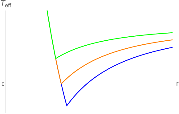
Figure 1: Effective tension as a function of the radius. The kink occurs at the corresponding junction position. Green, top: $r_{i}<r_{max}$ ($r_{e}>r_{i}$). Orange, middle: $r_{i}=r_{max}$ ($r_{e}=r_{i}$). Blue, bottom: $r_{i}>r_{max}$ ($r_{i}<r_{e}$).

So far we have shown that as long as $r_{i}\leq r_{max}$, we have $r_{i}\geq r_{e}$, and probe branes are well-behaved at any radial position. Moreover, the tension (82) decreases when approaching the junction from either side, reaching a minimum at $r=r_{i}$ (see Fig. 1). Although nothing dramatic occurs to the probes when they reach the junction if $r_{i}\neq r_{e}$, it is energetically favorable for them to stay there.

Among the possible $r_{i}\geq r_{max}$, it is natural to choose $r_{i}=r_{max}$, because that choice maximizes the region covered by the interior geometry. There is also a dynamical reason to take $r_{i}=r_{max}=r_{e}$, as only in this case do the branes at the junction become tensionless. Thus the configuration achieved for $r_{i}=r_{max}=r_{e}$ will have the least energy, and the branes at the junction will be uniformly distributed over the transverse $S^{3}$.

4.2 The $F1$-$NS5$ configuration

Our long detour to the S-dual picture has led us to a regularized geometry given in terms of the piecewise-defined harmonic functions (76), (77). We can now S-dualize back and study the implications for our original singular background (55), (56). After the S-duality transformation, we obtain

$$ds^{2} =f_{1}^{-1}\left(-dt^{2}+dx^{2}\right)+f_{5}\left(dr^{2}+r^{2}d\Omega_{3}^{2}\right)+V^{1/2}ds_{{\cal M}_{4}}^{2}$$ (87)

$$e^{2\Phi} =g_{s}\frac{f_{5}}{f_{1}}$$ (88)

with the harmonic functions given by

$$f_{1} =\begin{cases}1-\frac{r_{1-}^{2}+r_{1+}^{2}}{r_{i}^{2}}+\frac{r_{1-}^{2}}{r^{2}},&r<r_{i}\\ 1+\frac{r_{1+}^{2}}{r^{2}},&r>r_{i}\end{cases}$$ (89)

$$f_{5} =\begin{cases}1+\frac{r_{5+}^{2}-r_{5-}^{2}}{r_{i}^{2}}+\frac{r_{5-}^{2}}{r^{2}},&r<r_{i}\\ 1+\frac{r_{5+}^{2}}{r^{2}},&r>r_{i}\end{cases}$$ (90)

and with

$$r_{1-}^{2}=\frac{g_{s}^{2}\alpha^{\prime}Q_{1}}{v}\qquad ,\qquad r_{1+}^{2}=r_{1-}^{2}-\frac{g_{s}^{2}\alpha^{\prime}\delta N_{5}}{v}$$ (91)

$$r_{5-}^{2}=\alpha^{\prime}Q_{5}\qquad ,\qquad r_{5+}^{2}=r_{5-}^{2}+\alpha^{\prime}\delta N_{5}.$$ (92)

The relation (84), maximal incision (85) and the enhançon radius (81) are modified here by the appropriate powers of $g_{s}$.

To check that the above solution corresponds to our glued solution in the effective 3-dimensional theory, we perform the LST decoupling limit by taking $g_{s}\to 0$ after the change of variables $r^{2}=g_{s}^{2}\alpha^{\prime}u^{2}$ (together with the redefinition $r_{i}^{2}=g_{s}^{2}\alpha^{\prime}u_{i}^{2}$). We find:

$$f_{1} =\begin{cases}1-\frac{\delta N_{5}}{vu_{i}^{2}}+\frac{Q_{1}}{vu^{2}},&u<u_{i}\\ 1+\frac{Q_{1}-\delta N_{5}}{vu^{2}},&u>u_{i}\end{cases}$$ (93)

$$g_{s}^{2}f_{5} =\begin{cases}\frac{\delta N_{5}}{u_{i}^{2}}+\frac{Q_{5}}{u^{2}},&u<u_{i}\\ \frac{Q_{5}}{u^{2}}\,\,\,,&u>u_{i}\end{cases}.$$ (94)

Let us pause here to comment on the region in which this background is weakly coupled, or equivalently, where an analysis via perturbative string theory is valid. Evaluating the dilaton field of the above, it can be easily seen that for $Q_{1}>Q_{5}$ the effective string coupling is small all the way up from the deep IR ($u\to 0$) to $u\sim u_{i}$. Near the junction, the coupling diverges and the picture becomes untrustworthy. It is thus in the S-dual system that the string coupling becomes weak in that region, and the junction acquires a natural interpretation as a shell of $D5$-branes. In the exterior geometry of the NS case, a perturbative description is valid for sufficiently large values of $u$, as the system approaches a linear dilaton background.

Moving from this 10-dimensional picture down to the effective 3-dimensional theory amounts to following the steps listed in section 2. After changing coordinates from $u$ to $y$ with $vu^{2}=Q_{1}\lambda e^{2y}$, and redefining $vu_{i}^{2}=Q_{1}\lambda e^{2y_{i}}$, we arrive at the solution described in section 3. Finally, the relation (50) is no more than the matching condition (84) after the S-duality transformation and the subsequent change of coordinates described above.

With this 10-dimensional perspective, we see that the ability to find a 3-dimensional regular solution with a jump in flux parametrized by a single integer $\delta N_{5}$ is a manifestation of the fact that wrapping $D5$-branes on $K3$ generates an effective negative $D1$ tension and charge Bershadsky:1995qy ; Green_1997 ; Dasgupta_1998 ; Bachas_1999 ; Giddings:2001yu . Furthermore, the curious effect found in (48) can now be understood as a consequence of the presence of an enhançon scale in 10-dimensions. Thus, at least for the case where the compact manifold wrapped by the fivebranes is a $K3$, the singular behavior inherent to single-trace $T\bar{T}$-deformed backgrounds with negative $\lambda$ can be regularized by means of standard objects in type IIB string theory. The system maintains a strong resemblance to the well-understood physics of the enhançon mechanism.

Let us emphasize here that in this work we have achieved a particular UV completion, and other possibilities are by no means excluded. For instance, many of our considerations do not apply for the case when the Calabi-Yau 4-fold is a $T^{4}$, where a resolution might require involving unconventional string theory objects. We briefly comment on this situation in the next subsection.

4.3 $T^{4}$ and negative branes

Before moving forward, we relate our setup to an exotic UV completion which has been suggested in the recent literature Chakraborty:2020swe . We will perform a nontrivial analytic continuation of this system to reveal the singular geometries obtained above. We herein take $\delta N_{5}=0$ so that there is no change in the behavior of $f_{5}$ at the junction, and we furthermore define:

$$-1\equiv 1+\dfrac{r_{1+}^{2}-r_{1-}^{2}}{r_{i}^{2}}=1+\dfrac{V^{*}}{V}g_{s}\alpha^{\prime}\dfrac{\delta N_{1}}{r_{i}^{2}}.$$ (95)

For purposes of demonstration, fix $r_{i}$ in this expression. Then, taking $\lambda\to-\lambda$ (which gives the constant $-1$ in $f_{1}$) is equivalent to analytically continuing $\delta N_{1}$ to a negative value. Such a procedure is subtle, because the analytic continuation in $\lambda$ can be achieved by a marginal current-current deformation of the string worldsheet, which should not change the supersymmetries preserved by the background Petropoulos:2009jz . Thus the analytic continuation in $\delta N_{1}$ must be performed whilst fixing supersymmetries, i.e. the branes at the junction cannot possibly be anti-branes. Instead, they are objects with negative tension and negative charge which are BPS with the D-branes in the geometry.

This picture is analogous to the procedure used to derive the original enhançon geometry JPP , where the authors extend the exterior geometry to all $r$ and analytically continue $Q_{1+}$ to $-Q_{5+}$. They fix the same unbroken supersymmetries as in the $Q_{1+}>0$ case. In that context, it was by switching from a $T^{4}$ to a $K3$ compactification that the authors were able to avoid introducing an object with negative effective tension and recover the shell of branes. Due to the negative induced $D1$-brane charge that $D5$-branes carry when wrapped on $K3$ Bershadsky_1996 ; Green_1997 ; Dasgupta_1998 ; Bachas_1999 , these geometries can be generated from wrapped $D5$-branes alone. However, it is perfectly valid to insist on keeping the $T^{4}$.

To understand this geometry fully, we must rely on the negative-tension objects which are prescribed to us by the string theory literature. An option which was well-studied in Chakraborty:2020swe made use of so-called “negative branes,” which have SU$(0|M)$ gauge symmetry groups, i.e. their Chan-Paton factors are Grassmann numbers dijkgraaf2016negative . This option is certainly available for either choice of compactification manifold, but such objects tend to introduce exotic physics, such as signature changes and closed timelike curves. Notably, this option was also available in the original enhançon backgrounds. In that context, however, the restriction to the more standard taxonomy of extended objects in string theory uncovered elegant physics, and we therefore chose to restrict ourselves to these in this work.

There is one negative-tension, negative-charge candidate available to us in this scenario: orientifold planes, or $O1_{-}$-planes. These objects have no motion collective coordinates. They are nondynamical, because they introduce boundary conditions on the spacetime and fluxes which can be viewed (in a simplified sense) as a $\mathbb{Z}_{2}$ quotient of two copies of the system mirrored across the fixed plane. Orientifolds have been considered as an extension of the original enhançon results, in Jarv:2000zv . We have restricted the scope of this initial work to a resolution via branes, but we find the prospect of a compactification via $O$-planes tantalizing, and we hope to address it in subsequent work.

5 Comments on the spectrum of excited states

In this last section, we briefly expand on some ideas which may provide a more complete insight about the nature of the regular backgrounds studied so far.

In particular, the glued geometry constructed in sections 3 and 4 corresponds to the deformation of the RR vacuum state, and thus looks like the pure $AdS_{3}$ vacuum at small enough radial positions. The spectrum of low energy excitations above the undeformed ($AdS_{3}$) vacuum can be obtained by studying the dynamics of long strings on top of it. The latter amounts to considering the (spectrally flowed) continuous representations of $SL(2,\mathbb{R})$ Maldacena:2000hw . The excitations of the untwisted sector can be thought of as corresponding to the dynamics of a single block in the dual orbifold CFT. The spectrum of such long string states has been computed exactly in the single-trace $T\bar{T}$-deformed vacuum using standard techniques in Apolo:2019zai . This is possible because the deformed worldsheet sigma model remains solvable for any value of the deformation parameter. Unfortunately, in our setting, although the calculation remains the same in a portion of the interior geometry, the backgrounds presented herein do not correspond to the conventional single-trace $T\bar{T}$ deformation. Rather, they correspond to a more complicated trajectory in the space of QFT’s, which is still unknown to us. The absence of singularities in our backgrounds is a strong indication of the avoidance of complex energy levels above a certain cutoff scale.

We can nevertheless characterize the dominant contributions of this flow in different energy regimes. At low energies, we can argue that the spectrum of long strings stretched at radial distances lying well below the scale $y_{IR}$ introduced in section 3 must coincide with the $T\bar{T}$-deformed spectrum with negative coupling in a single block of the deformed orbifold QFT. This statement comes naturally from the fact that the sigma model is still solvable in this region, as explained above. Moreover, by means of expression (54), the region of analytic control can in principle be enlarged at will by considering a certain double-scaled limit in which $Q_{1}\to\infty$, $\lambda\to 0$ with $\lambda Q_{1}\ll Q_{5}$.

In the other extreme regime, we might consider very massive states which, as usual, are not described by perturbative dynamics, but by black holes. Obtaining consistent black hole states for these sort of glued constructions is a challenging task in the context of the enhançon mechanism, and was studied in Johnson:2001wm ; Dimitriadis:2003ur ; Dimitriadis:2002xd ; Dimitriadis:2003ya . This difficulty can in principle be attributed to a number of ambiguities which arise when determining the actual geometry associated to these states. One of the most severe ambiguities resides in the presence of two horizons, respectively for the interior and exterior geometries. In principle, there is no further insight from the supergravity equations which allows us to fix a particular relation between these parameters, which is an obstruction to determining their thermodynamics. Quite importantly, a branch of these solutions has been shown to violate the Weak Energy Condition in a broad regime of parameter space, being therefore characterized as unphysical Dimitriadis:2003ur ; Dimitriadis:2003ya .

Thus a generic treatment of black hole solutions over these backgrounds is beyond the scope of this work. It might be argued that the knowledge of the dynamics of the holographic IR CFT may provide some insight to overcome these issues, and that would be an interesting idea to pursue in future work. For now, we will instead focus on the particular cases which are free of such ambiguities: namely heavy states lying in the upper region of the mass spectrum. More concretely, solutions featuring a large horizon radius are simple in the sense that any subtlety related to the interior geometry or the details of the junction can be disregarded once the interior region lies completely within the horizon. The thermodynamics associated to these configurations therefore only care about the exterior geometry. The validity of these solutions is guaranteed as long as they do not develop an enhançon radius outside the horizon, as we will comment below.

For concreteness, we will consider non-rotating charged black hole solutions. The charges correspond to the ones present on the exterior region, namely $Q_{1}^{ext}=Q_{1}-\delta N_{5}\equiv\tilde{Q}_{1}$, $Q_{5}^{ext}=Q_{5}+\delta N_{5}\equiv\tilde{Q}_{5}$. The string frame metric reads

$$ds^{2}=h_{1}^{-1}(-Kdt^{2}+dx^{2})+h_{5}(K^{-1}dr^{2}+r^{2}d\Omega_{3}^{2})+V^{1/2}ds^{2}_{K3}$$ (96)

where

$$h_{1}=1+\frac{\hat{r}_{1}^{2}}{r^{2}}\,\,\,,\,\,\,h_{5}=1+\frac{\hat{r}_{5}^{2}}{r^{2}}\,\,\,,\,\,\,K=1-\frac{r_{0}^{2}}{r^{2}}$$ (97)

with $\hat{r}_{1}$ and $\hat{r}_{5}$ given by

$$\hat{r}_{1}^{2}=r_{0}^{2}\sinh^{2}\alpha_{1}\,\,\, ,\,\,\,\hat{r}_{5}^{2}=r_{0}^{2}\sinh^{2}\alpha_{5}$$

$$\sinh{2\alpha_{1}}=\frac{2g_{s}^{2}\alpha^{\prime}\tilde{Q}_{1}}{vr_{0}^{2}}\,\,\, ,\,\,\,\sinh{2\alpha_{5}}=\frac{2\alpha^{\prime}\tilde{Q}_{5}}{r_{0}^{2}}.$$ (98)

The dilaton and 3-form fluxes depend on the harmonic functions in the same way as for the extremal solutions, so we do not write them here.

The thermodynamics associated to these configurations has recently been studied in Chakraborty:2020swe , as they are associated to very massive states in positive coupling single trace $T\bar{T}$. As our geometries have the same asymptotic behaviour in the UV region, the conclusions of Chakraborty:2020swe carry over to those same high-energy states here. As the relevant computations have been already performed in Chakraborty:2020swe , we limit ourselves to report the relevant results here. To keep our discussion self-contained, we show some details of the calculation in Appendix C.

We will work in the decoupling limit, for which $\alpha_{5}\to\infty$ while $\alpha_{1}$ is kept fixed. The entropy as a function of the dimensionless energy above extremality ${\cal E}$ (see Appendix C) is accounted by the area of the compact horizon at $r=r_{0}$ and reads

$$S=2\pi\sqrt{\tilde{Q}_{5}}\sqrt{2\tilde{Q}_{1}{\cal E}+\lambda{\cal E}}$$ (99)

hence making manifest that the dynamics of high energy states interpolates between the usual Cardy regime and the Hagedorn growth, with the entropy reaching its maximum at the critical energy

$${\cal E}_{c}=\frac{\tilde{Q}_{1}}{\lambda}.$$ (100)

For energies above this scale, the effective temperature becomes negative and the theory becomes highly non-local. We emphasize that none of the results stated above are new. We reproduce them here to illustrate the dynamics associated to high energy states in our setup, and to connect the resolved geometries presented herein to previous work.

It is instructive to compute the minimal energy for which these considerations are valid. This amounts to computing the particular value of ${\cal E}$ for which the horizon $r_{0}$ meets an enhançon radius. To find the enhançon radius in this context, we have to go again to the S-dual geometry. Notice that the probe brane analysis is no longer insightful, as there is a nontrivial potential for the brane motion, due to the absence of supersymmetry. However, one can still define the enhançon as the radial position at which the $K3$ becomes of the string scale, so obtaining

$$\hat{r}^{2}_{e}=\frac{\hat{r}_{5}^{2}-v\hat{r}_{1}^{2}}{v-1}$$ (101)

where, in an abuse of notation, we are denoting by $\hat{r}_{1}$, $\hat{r}_{5}$ to the corresponding S-dual quantities. By S-dualizing back, we get

$$\hat{r}^{2}_{e}=\frac{1}{v-g_{s}^{2}}\left(g_{s}^{2}\hat{r}_{5}^{2}-v\hat{r}_{1}^{2}\right)$$ (102)

and, taking the decoupling limit and expressing all quantities in terms of the energy above extremality, we finally obtain

$$\frac{\hat{r}_{e}^{2}}{r_{0}^{2}}=\frac{\tilde{Q}_{5}(\tilde{Q}_{1}+\lambda{\cal E})-\tilde{Q}_{1}^{2}}{\lambda{\cal E}(2\tilde{Q}_{1}+\lambda{\cal E})}.$$ (103)

From this, we derive the minimal energy condition as:

$$\frac{\hat{r}_{e}^{2}}{r_{0}^{2}}<1\,\,\,\Rightarrow\,\,\,{\cal E}>{\cal E}_{min}$$ (104)

with

$${\cal E}_{min}=\frac{\tilde{Q}_{5}-\tilde{Q}_{1}}{\lambda}=\frac{Q_{5}-Q_{1}+2\delta N_{5}}{\lambda}$$ (105)

The above quantity hence represents the minimal energy for which the large horizon analysis presented so far holds. To understand what happens at scales below (105), one needs a consistent glued black hole solution, featuring interior and exterior horizons and merging at a given radial position. As explained previously, those solutions are subtle, so we leave a more thorough analysis of this region of the spectrum to future work.

6 Discussion

In this work, we constructed a family of regular solutions of type IIB supergravity with Neveu-Schwartz flux which resolve the naked singularity in single-trace $T\bar{T}$-deformed backgrounds. The resolution procedure has some direct connections with the enhançon mechanism, previously considered in the literature to resolve repulson-type singularities JPP ; Johnson:2001wm . Even though we reproduce the single-trace $T\bar{T}$-deformed background in the IR region, the solutions considered here do not correspond holographically to the same flow in the space of QFT’s. In particular, the avoidance of curvature and dilaton singularities, as well as the absence of closed timelike curves, signal that this flow can be traced all the way to the UV region without developing complex energy levels. In the UV, the theory becomes non-local and develops Hagedorn scaling in the density of states. This is clear if one observes that the supergravity background reduces to a linear dilaton vacuum of Little String Theory in the asymptotic region.

It is important to comment on the indirect nature of the mechanism we have proposed. In particular, because the effective string coupling in the NS-NS case grows strong near the singularity, a trustworthy description is only achieved by S-dualizing to a background featuring R-R fluxes. It is in this S-dual system that the physics of D-branes wrapped on $K3$ allows for a resolution via the enhançon construction. This is the only consistent mechanism we have identified in which the singularity is resolved by standard dynamics in string theory; that is, without appealing to any exotic soliton to account for negative tensions. Let us nevertheless emphasize that a more direct resolution concerning the dynamics of fundamental strings and $NS5$-branes would be very interesting to achieve. The highly non-trivial action functional of $NS5$-brane probes makes this task computationally challenging.

Another exciting and in principle affordable possibility is to find a consistent truncation of the radial direction within a warped compactification Randall:1999ee ; Randall:1999vf . Achieving this may establish a non-trivial connection between single-trace $T\bar{T}$ and the finite cut-off holographic realization of double-trace $T\bar{T}$ MMV . Accordingly, it may also be more natural to construct a “single-trace” analogy of the “$T\bar{T}\,+\,\Lambda_{2}$” flows recently introduced in Gorbenko:2018oov , interpolating between globally AdS and dS spacetimes, given that dS is already compact in the spatial directions. We hope to address this point in the near future.

Finally, within the context of the combined flows studied in this paper, there are two important gaps to be filled. One is to perform a more systematic study of black hole solutions joined at a finite radial position, in order to describe the dynamics of intermediate energy states. The other is to obtain these geometries from the worldsheet perspective—that is, to find a particular (and hopefully solvable) deformation of the string sigma model featuring these geometries as solutions of the field equations.

Appendix A Derivation of repulson behavior

Technically, for the enhançon mechanism to activate, we only need the running $K3$ volume to reach $V^{*}=(4\pi^{2}\alpha^{\prime})^{2}$ at some locus in the string frame geometry. As far as the initial enhançon results JPP are concerned, this behavior defines a repulson-type singularity. However, such a characterization raises concern for the interpretation of the singularity in the NS-NS sector, where the running $K3$ volume is constant. Here, we will confirm the repulson-type behavior by studying the original definition, which depends only on characteristics of the Einstein frame metric and is therefore unaffected by an S-duality transformation. The first works on repulsons Repulson1 ; Repulson2 ; Repulson3 characterized their backgrounds of interest by studying the classical behavior of matter moving toward the singularity from the well-behaved region. As described in detail in Repulson2 , the effective gravitational potential grows positive and becomes infinite as a massive test particle approaches the singularity. The particle is inevitably repelled, hence the name “repulson.” These analyses (c.f. section 5 of Repulson2 ) closely followed a textbook derivation from section 98 of landau1975classical . We will go through it here, both for the geometry in the original enhançon results, as well as for our system of interest.

In Einstein frame, the generic $D1$-$D5$ background (equivalently, $F1$-$NS5$ background) is rotationally invariant and has a timelike Killing vector, so the energy $E$ and momenta $P_{i}$ of the particle will be conserved. For simplicity, we will neglect momenta along $K3$ and $S^{3}$, and instead allow only for angular momentum $L$ around $x$. The equation of state for the system is

$$S=-Et+Lx+S_{r}(r),\qquad\qquad g^{\mu\nu}\dfrac{\partial S}{\partial x^{\mu}}\dfrac{\partial S}{\partial x^{\nu}}=m^{2}.$$ (106)

This presents a differential equation for $S_{r}$, which we can solve with

$$S_{r}(r)=\pm\int_{r_{0}}^{r}dr^{\prime}\sqrt{-\dfrac{g_{rr}}{g_{tt}g_{xx}}\left(E^{2}g_{xx}+m^{2}g_{tt}g_{xx}+L^{2}g_{tt}\right)}.$$ (107)

Plugging this into $S$, we can now impose the Hamilton-Jacobi equation $\frac{\partial S}{\partial E}=0$. This gives us a relation between $r$ and $t$:

$$t=\int^{r}_{r_{0}}dr^{\prime}\,\frac{Er^{\prime}}{\sqrt{-g_{tt}\left(E^{2}g_{rr}+m^{2}g_{tt}g_{rr}+L^{2}\frac{g_{tt}}{g_{xx}}g_{rr}\right)}},$$ (108)

where the sign is fixed in this case by specifying that the particle starts from some radius $r_{0}$ far away from the singularity and falls in toward it. This is equivalent to (46) in Repulson2 , where in that case $\frac{g_{rr}}{g_{xx}}=\frac{1}{r^{2}}$ and they take $g_{tt}=g_{xx}$ (i.e. they drop the sign difference). The simple way to view the repulson behavior in this expression is to note for what values of $r$ the denominator is pure complex. Generically, this will occur at some radius before the particle hits the singularity, irrespective of energy or angular momentum. Rather than a point of no return (an event horizon), there is a point of no advance, which the authors of Repulson2 referred to as “antigravity.”

In 10 dimensions, the Einstein frame metric has

$$g_{rr}=f_{1}^{1/4}f_{5}^{3/4},\qquad g_{xx}=-g_{tt}=f_{1}^{-3/4}f_{5}^{-1/4},$$ (109)

and the integrand takes the form

$$\dfrac{Ef_{1}^{5/8}f_{5}^{7/8}}{\sqrt{(E^{2}-L^{2})f_{1}^{1/4}f_{5}^{3/4}-m^{2}\sqrt{\frac{f_{5}}{f_{1}}}}}.$$ (110)

As we move toward the singularity, $f_{1}$ shrinks to $0$ whereas $f_{5}$ does not. For $m\neq 0$ the argument to the square root in the denominator eventually becomes negative, irrespective of the energy $E$. Thus the repulson behavior is visible both for the original enhançon geometry with $f_{i}=\bar{Z}_{i}$ in (62) as well as the deformed geometry with $f_{i}$ in (56). The exact radii where the integrands become complex are attainable for both systems, although they have complicated and unenlightening forms.

The massless case requires special treatment. We write the proper velocity $U$ as

$$U_{\mu}=\begin{pmatrix}E\\ L\\ U_{r}\end{pmatrix}.$$ (111)

Enforcing $g_{\mu\nu}U^{\mu}U^{\nu}=0$ allows us to solve for $U_{r}$ in terms of $E,L$ and $r$. The proper velocity and acceleration, with affine parameter $\xi$, is

$$U^{r} =\dfrac{\partial r}{\partial\xi}=\pm\sqrt{E^{2}-L^{2}}\left(\dfrac{f_{1}}{f_{5}}\right)^{1/4}$$ (112)

$$\partial_{\xi}U^{r} =\mp(E^{2}-L^{2})\dfrac{r_{1}^{2}+r_{5}^{2}}{2r^{3}f_{1}^{1/2}f_{5}^{3/2}}$$ (113)

It is clear that the maximum value of $r(\xi)$ is the radius where $f_{1}$ vanishes, and that the singularity repels the geodesics with diverging strength as they approach the singularity.

A subtlety in the dimensional reduction

There is a slight subtlety in the definition of repulson used above, as the Weyl factor used to derive the Einstein frame metric depends on the number of dimensions we choose to compactify. To illustrate this nuance, let us consider the system in only the $t,r,x$ coordinates and compactify the $S^{3}\times{\cal M}_{4}$. Then:

$$g_{rr}=f_{1}^{-3/4}f_{5}^{5/4},\qquad g_{xx}=-g_{tt}=f_{1}^{-5/4}f_{5}^{3/4},$$ (114)

and one finds that the integrand in (108) instead becomes

$$\dfrac{E(f_{1}f_{5})^{7/8}}{\sqrt{(E^{2}-L^{2})(f_{1}f_{5})^{5/4}-m^{2}f_{5}^{2}}}$$ (115)

Massive particles will still not be able to reach the singularity in finite time. However, we argue that the most sensible definition of repulson behavior is the one which makes use of the 10-dimensional geometry, i.e. without any compactification. This convention minimizes ambiguity, although it is different from the one in Repulson2 .

Appendix B Probe brane computation

We are interested in a $D5$-brane probe on a background of the form

$$ds^{2} =Z_{1}^{-1/2}Z_{5}^{-1/2}(-dt^{2}+dx^{2})+Z_{1}^{1/2}Z_{5}^{1/2}(dr^{2}+r^{2}d\Omega_{3}^{2})+Z_{1}^{1/2}Z_{5}^{-1/2}V^{1/2}ds^{2}_{{\cal M}_{4}}$$ (116)

$$e^{2\tilde{\Phi}} =g_{s}\frac{Z_{1}}{Z_{5}}\,\,\,,\,\,\,C_{2}=Z_{1}^{-1}dt\wedge dx\,\,\,,\,\,\,C_{6}=Z_{5}^{-1}dt\wedge dx\wedge V\epsilon_{K3}$$ (117)

where $\epsilon_{K3}$ is the volume form on the unit $K3$.

The probe will be wrapped over the $K3$ and extended on the non-compact $t$ and $x$ directions. By fixing the static gauge, we identify the world volume coordinates

$$\{\zeta^{a}\}=\{t,x,K3\}$$ (118)

Moreover, we will only consider time dependence in the transverse directions.

For the induced metric on the world volume we obtain

$$g_{tt} =-Z_{1}^{-1/2}Z_{5}^{-1/2}+Z_{1}^{1/2}Z_{5}^{1/2}v_{T}^{2}$$ (119)

$$g_{xx} =Z_{1}^{-1/2}Z_{5}^{-1/2}$$ (120)

$$g_{ij} =V^{1/2}Z_{1}^{1/2}Z_{5}^{-1/2}g^{K3}_{ij}\,\,\,,\,\,\,\{i,j\in K3\}$$ (121)

where we have defined the transverse velocity $v_{T}^{2}=\dot{r}^{2}+r^{2}(\dot{\theta}^{2}+\sin^{2}\theta\dot{\varphi}_{1}^{2}+\sin^{2}\theta\sin^{2}\varphi_{1}\dot{\varphi}_{2}^{2})$ and the angles $\{\theta,\varphi_{1},\varphi_{2}\}$ are coordinates on the 3-sphere. Therefore, in a slow-moving approximation, we have

$$\sqrt{-\det g}=\frac{V}{Z_{5}}\sqrt{\frac{Z_{1}}{Z_{5}}}\sqrt{1-Z_{1}Z_{5}v_{T}^{2}}\sqrt{\det g^{K3}}\approx\frac{V}{Z_{5}}\sqrt{\frac{Z_{1}}{Z_{5}}}\sqrt{\det g^{K3}}\left(1-\frac{Z_{1}Z_{5}v_{T}^{2}}{2}\right).$$ (122)

With the above expression in hand, we can evaluate the DBI action (note that we are setting the internal $U(1)$ gauge field to zero):

$$S_{DBI}=-T_{5}\int d^{6}\zeta\,e^{-\Phi}\sqrt{-\det g}\approx-T_{5}\int dt\,\frac{V}{Z_{5}}\left(1-\frac{Z_{1}Z_{5}v^{2}}{2}\right).$$ (123)

Now we proceed to evaluate the WZW coupling of the $D5$-brane to the 6-form flux. The latter has no transverse components, so the pullback is trivial, giving

$$S_{WZW}=T_{5}\int d^{6}\zeta\,C_{6}=T_{5}\int dt\,\frac{V}{Z_{5}}.$$ (124)

However, here certain stringy effects must be taken into account. As explained in Bershadsky:1995qy (and reviewed in first section of Giddings:2001yu ), by anomaly inflow there is an additional WZW coupling when wrapping a $D5$-brane on $K3$. This additional contribution is proportional to $\alpha^{\prime 2}$ and roughly takes the form

$$\delta S_{WZW}\sim T_{5}\alpha^{\prime 2}\int_{WV}C_{2}\wedge p_{1}(K3),$$ (125)

where $p_{1}$ denotes the first Pontryagin class of $K3$. Given that $C_{2}$ does not have any component on $K3$, and since $p_{1}$ is quantized to a negative integer, it turns out that

$$\delta S_{WZW}=-T_{1}\int dt\,Z_{1}^{-1}.$$ (126)

Note the absence of a factor of $V$, given that $p_{1}$ is a topological invariant and, as such, is independent of the overall volume of $K3$. Here we have used that $T_{1}/T_{5}=(2\pi)^{4}\alpha^{\prime 2}$.

Since the configuration is still BPS, the tension has to acquire a compensating term of the same form. By the above reasoning, this new term does not have any factor of $V$ either. Thus the relevant induced metric is the one corresponding to the subspace spanned by $t,x$, giving

$$\delta S_{DBI}=T_{1}\int d^{2}\zeta e^{-\Phi}\sqrt{-\det g^{(t,x)}}\approx T_{1}\int dt\frac{1}{Z_{1}}\left(1-\frac{Z_{1}Z_{5}v_{T}^{2}}{2}\right).$$ (127)

Putting all together we get

$${\cal L}_{probe} \approx\left(-T_{5}VZ_{5}^{-1}+T_{1}Z_{1}^{-1}\right)\left(1-\frac{Z_{1}Z_{5}v_{T}^{2}}{2}\right)+T_{5}VZ_{5}^{-1}-T_{1}\tilde{Z}_{1}^{-1}$$ (128)

$$=\frac{1}{2}\left(T_{5}VZ_{1}-T_{1}Z_{5}\right)v_{T}^{2},$$ (129)

hence the effective tension reads

$$T_{eff}=T_{1}\left(\frac{T_{5}}{T_{1}}VZ_{1}-Z_{5}\right),$$ (130)

as quoted in the main text.

Appendix C Computation of the black hole entropy

To keep the presentation self-contained, we review the basics of the computation done in Chakraborty:2020swe which leads to the entropy (99). As explained in section 5, for sufficiently large mass, the relevant black hole solutions do not feature an enhançon occurring outside the horizon, hence only the exterior geometry matters for describing their thermodynamics.

It is natural to dimensionally reduce to five dimensions, where the Einstein frame metric reads

$$ds^{2}=-(h_{1}h_{5})^{-2/3}Kdt^{2}+(h_{1}h_{5})^{1/3}(K^{-1}dr^{2}+r^{2}d\Omega_{3}),$$ (131)

with the harmonic functions $f_{1}$, $f_{5}$ and emblackening factor $K$ given in (97), (98).

The energy associated to these configurations is accounted for by the ADM mass. The latter can be read off from the asymptotic structure of the metric:

$$g_{tt}=-1+\frac{8G_{N}^{5d}}{3\pi}\frac{M}{r^{2}}+{\cal O}(r^{-4})\,,$$ (132)

which in this case yields

$$M=\frac{3\pi}{8G_{N}^{5d}}\frac{2}{3}(\hat{r}_{1}^{2}+\hat{r}_{5}^{2}+\frac{3}{2}r_{0}^{2})=\frac{vRr_{0}^{2}}{2g_{s}^{2}\alpha^{\prime 2}}(\cosh 2\alpha_{1}+\cosh{2\alpha_{5}}+1)\,,$$ (133)

and we have used the five-dimensional Newton’s constant of the form

$$G_{N}^{5d}=\frac{G_{N}^{(10)}}{V(2\pi R)}=\frac{\pi g_{s}^{2}\alpha^{\prime 2}}{4vR}.$$ (134)

The extremal mass is readily obtained by taking $r_{0}\to 0$, giving

$$M^{ext}=\frac{vR}{g_{s}^{2}\alpha^{\prime}}(\frac{g_{s}^{2}}{v}\tilde{Q}_{1}+\tilde{Q}_{5}).$$ (135)

The energy above extremality then reads

$$E=M-M^{ext}\frac{vR\tilde{r}_{0}^{2}}{2g_{s}^{2}\alpha^{\prime 2}}\left(e^{-2\alpha_{1}}+e^{-2\alpha_{5}}+1\right).$$ (136)

As explained in the main text, we take the decoupling limit, by which $\alpha_{5}\to\infty$ while $\alpha_{1}$ is kept fixed. In this limit, the dimensionless energy reads as follows

$${\cal E}\equiv RE=\frac{vR^{2}r_{0}^{2}}{2g_{s}^{2}\alpha^{\prime 2}}\left(e^{-2\alpha_{1}^{+}}+1\right)=\frac{\tilde{Q}_{1}}{\lambda\sinh 2\alpha_{1}^{+}}\left(e^{-2\alpha_{1}^{+}}+1\right).$$ (137)

Note we have rewritten the horizon radius in terms of $\alpha_{1}$ by means of (98) and also introduced the deformation parameter $\lambda=\alpha^{\prime}/R$.

Finally, the entropy associated to the solution is obtained by computing the area spanned by the $S^{3}$ at the horizon $r=r_{0}$. From (131) one easily obtains

$$S=\frac{{\rm Area}(S^{3})}{4G_{N}^{5d}}=\frac{2\pi vRr_{0}^{3}}{g_{s}^{2}\alpha^{\prime 2}}\cosh\alpha_{1}\cosh{\alpha_{5}}\approx\frac{2\pi vR\sqrt{\tilde{Q}_{5}}r_{0}^{2}}{g_{s}^{2}\alpha^{\prime 3/2}}\cosh\alpha_{1}$$ (138)

where, in going to the second equality, we have taken the decoupling limit. Finally, inverting the relation (137) and plugging it into the above expression, one gets the equation of state (99) for the entropy in terms of the energy above extremality.

References

- (1) A.B. Zamolodchikov, Expectation value of composite field T anti-T in two-dimensional quantum field theory, hep-th/0401146.
- (2) F. Smirnov and A. Zamolodchikov, On space of integrable quantum field theories, Nuclear Physics B 915 (2017) 363–383.
- (3) A. Cavaglià, S. Negro, I.M. Szécsényi and R. Tateo, -deformed 2D Quantum Field Theories, JHEP 10 (2016) 112 [1608.05534].
- (4) J. Cardy, The deformation of quantum field theory as random geometry, JHEP 10 (2018) 186 [1801.06895].
- (5) J. Cardy, deformation of correlation functions, JHEP 19 (2020) 160 [1907.03394].
- (6) W. Donnelly and V. Shyam, Entanglement entropy and deformation, Phys. Rev. Lett. 121 (2018) 131602 [1806.07444].
- (7) Y. Jiang, Lectures on solvable irrelevant deformations of 2d quantum field theory, 1904.13376.
- (8) S. Dubovsky, R. Flauger and V. Gorbenko, Solving the Simplest Theory of Quantum Gravity, JHEP 09 (2012) 133 [1205.6805].
- (9) S. Dubovsky, V. Gorbenko and M. Mirbabayi, Asymptotic fragility, near AdS2 holography and , JHEP 09 (2017) 136 [1706.06604].
- (10) S. Dubovsky, V. Gorbenko and G. Hernández-Chifflet, partition function from topological gravity, JHEP 09 (2018) 158 [1805.07386].
- (11) E.A. Coleman, J. Aguilera-Damia, D.Z. Freedman and R.M. Soni, -deformed actions and (1,1) supersymmetry, JHEP 10 (2019) 080 [1906.05439].
- (12) A.J. Tolley, deformations, massive gravity and non-critical strings, JHEP 06 (2020) 050 [1911.06142].
- (13) E.A. Mazenc, V. Shyam and R.M. Soni, A Deformation for Curved Spacetimes from 3d Gravity, 1912.09179.
- (14) L. McGough, M. Mezei and H. Verlinde, Moving the CFT into the bulk with , JHEP 04 (2018) 010 [1611.03470].
- (15) P. Kraus, J. Liu and D. Marolf, Cutoff AdS3 versus the deformation, JHEP 07 (2018) 027 [1801.02714].
- (16) V. Gorbenko, E. Silverstein and G. Torroba, dS/dS and , JHEP 03 (2019) 085 [1811.07965].
- (17) A. Lewkowycz, J. Liu, E. Silverstein and G. Torroba, and EE, with implications for (A)dS subregion encodings, JHEP 04 (2020) 152 [1909.13808].
- (18) T. Hartman, J. Kruthoff, E. Shaghoulian and A. Tajdini, Holography at finite cutoff with a deformation, JHEP 03 (2019) 004 [1807.11401].
- (19) M. Guica and R. Monten, and the mirage of a bulk cutoff, 2019.
- (20) E. Coleman and V. Shyam, Conformal Boundary Conditions from Cutoff AdS3, 2010.08504.
- (21) A. Giveon, D. Kutasov and N. Seiberg, Comments on string theory on AdS(3), Adv. Theor. Math. Phys. 2 (1998) 733 [hep-th/9806194].
- (22) D. Kutasov and N. Seiberg, More comments on string theory on AdS(3), JHEP 04 (1999) 008 [hep-th/9903219].
- (23) N. Seiberg and E. Witten, The D1 / D5 system and singular CFT, JHEP 04 (1999) 017 [hep-th/9903224].
- (24) R. Argurio, A. Giveon and A. Shomer, Superstrings on AdS(3) and symmetric products, JHEP 12 (2000) 003 [hep-th/0009242].
- (25) L. Eberhardt, M.R. Gaberdiel and R. Gopakumar, The Worldsheet Dual of the Symmetric Product CFT, JHEP 04 (2019) 103 [1812.01007].
- (26) L. Eberhardt, M.R. Gaberdiel and R. Gopakumar, Deriving the AdS3/CFT2 correspondence, JHEP 02 (2020) 136 [1911.00378].
- (27) M.R. Gaberdiel, R. Gopakumar, B. Knighton and P. Maity, From Symmetric Product CFTs to , 2011.10038.
- (28) O. Aharony, M. Berkooz, D. Kutasov and N. Seiberg, Linear dilatons, NS five-branes and holography, JHEP 10 (1998) 004 [hep-th/9808149].
- (29) E. Witten, New ’gauge’ theories in six-dimensions, JHEP 01 (1998) 001 [hep-th/9710065].
- (30) A. Giveon, D. Kutasov, E. Rabinovici and A. Sever, Phases of quantum gravity in AdS(3) and linear dilaton backgrounds, Nucl. Phys. B 719 (2005) 3 [hep-th/0503121].
- (31) A. Giveon, N. Itzhaki and D. Kutasov, and LST, JHEP 07 (2017) 122 [1701.05576].
- (32) A. Giveon, N. Itzhaki and D. Kutasov, A solvable irrelevant deformation of AdS3/CFT2, JHEP 12 (2017) 155 [1707.05800].
- (33) M. Asrat, A. Giveon, N. Itzhaki and D. Kutasov, Holography Beyond AdS, Nucl. Phys. B932 (2018) 241 [1711.02690].
- (34) S. Chakraborty, A. Giveon and D. Kutasov, , Black Holes and Negative Strings, 2006.13249.
- (35) R. Dijkgraaf, B. Heidenreich, P. Jefferson and C. Vafa, Negative branes, supergroups and the signature of spacetime, 2016.
- (36) S. Chakraborty, A. Giveon and D. Kutasov, Strings in irrelevant deformations of AdS3/CFT2, JHEP 11 (2020) 057 [2009.03929].
- (37) J. McGreevy and E. Silverstein, The tachyon at the end of the universe, Journal of High Energy Physics 2005 (2005) 090–090.
- (38) M.S. Costa, C.A. Herdeiro, J. Penedones and N. Sousa, Hagedorn transition and chronology protection in string theory, Nuclear Physics B 728 (2005) 148–178.
- (39) L. Dixon, J. Harvey, C. Vafa and E. Witten, Strings on orbifolds, Nuclear Physics B 261 (1985) 678 .
- (40) E. Witten, Phases of N=2 theories in two-dimensions, AMS/IP Stud. Adv. Math. 1 (1996) 143 [hep-th/9301042].
- (41) P.S. Aspinwall, B.R. Greene and D.R. Morrison, Multiple mirror manifolds and topology change in string theory, Phys. Lett. B 303 (1993) 249 [hep-th/9301043].
- (42) A. Strominger, Massless black holes and conifolds in string theory, Nucl. Phys. B 451 (1995) 96 [hep-th/9504090].
- (43) B.R. Greene, D.R. Morrison and A. Strominger, Black hole condensation and the unification of string vacua, Nucl. Phys. B 451 (1995) 109 [hep-th/9504145].
- (44) K. Behrndt, About a class of exact string backgrounds, Nucl. Phys. B455 (1995) 188 [hep-th/9506106].
- (45) R. Kallosh and A.D. Linde, Exact supersymmetric massive and massless white holes, Phys. Rev. D52 (1995) 7137 [hep-th/9507022].
- (46) M. Cvetic and D. Youm, Singular BPS saturated states and enhanced symmetries of four-dimensional N=4 supersymmetric string vacua, Phys. Lett. B359 (1995) 87 [hep-th/9507160].
- (47) S. Chakraborty, A. Giveon and D. Kutasov, , , and String Theory, 1905.00051.
- (48) J.M. Maldacena and H. Ooguri, Strings in AdS(3) and SL(2,R) WZW model 1.: The Spectrum, J. Math. Phys. 42 (2001) 2929 [hep-th/0001053].
- (49) S. Hassan and A. Sen, Marginal deformations of WZNW and coset models from O(d,d) transformation, Nucl. Phys. B 405 (1993) 143 [hep-th/9210121].
- (50) T. Araujo, E. Colgáin, Y. Sakatani, M. Sheikh-Jabbari and H. Yavartanoo, Holographic integration of \& via , JHEP 03 (2019) 168 [1811.03050].
- (51) D. Israel, C. Kounnas and M.P. Petropoulos, Superstrings on NS5 backgrounds, deformed AdS(3) and holography, JHEP 10 (2003) 028 [hep-th/0306053].
- (52) C.V. Johnson, A.W. Peet and J. Polchinski, Gauge theory and the excision of repulson singularities, Phys. Rev. D61 (2000) 086001 [hep-th/9911161].
- (53) C.V. Johnson, R.C. Myers, A.W. Peet and S.F. Ross, The Enhancon and the consistency of excision, Phys. Rev. D 64 (2001) 106001 [hep-th/0105077].
- (54) N. Seiberg and E. Witten, Electric - magnetic duality, monopole condensation, and confinement in N=2 supersymmetric Yang-Mills theory, Nucl. Phys. B 426 (1994) 19 [hep-th/9407087].
- (55) A.W. Peet, Excision of ‘repulson’ singularities: A Space-time result and its gauge theory analog, in 7th International Symposium on Particles, Strings and Cosmology, pp. 82–90, 12, 1999, DOI [hep-th/0003251].
- (56) G.L. Alberghi, S. Corley and D.A. Lowe, Moduli space metric of N=2 supersymmetric SU(N) gauge theory and the enhancon, Nucl. Phys. B 635 (2002) 57 [hep-th/0204050].
- (57) F. Benini, M. Bertolini, C. Closset and S. Cremonesi, The N=2 cascade revisited and the enhancon bearings, Phys. Rev. D 79 (2009) 066012 [0811.2207].
- (58) N.R. Constable, The Entropy of 4-D black holes and the enhancon, Phys. Rev. D 64 (2001) 104004 [hep-th/0106038].
- (59) A. Dimitriadis and S.F. Ross, Stability of the nonextremal enhancon solution. 1. Perturbation equations, Phys. Rev. D 66 (2002) 106003 [hep-th/0207183].
- (60) A. Dimitriadis and S.F. Ross, Properties of nonextremal enhancons, Phys. Rev. D 69 (2004) 026002 [hep-th/0307216].
- (61) A. Dimitriadis, A.W. Peet, G. Potvin and S.F. Ross, Enhancon solutions: Pushing supergravity to its limits, Phys. Rev. D 70 (2004) 046001 [hep-th/0311271].
- (62) C.V. Johnson and R.C. Myers, The Enhancon, black holes, and the second law, Phys. Rev. D64 (2001) 106002 [hep-th/0105159].
- (63) M. Bershadsky, C. Vafa and V. Sadov, D-branes and topological field theories, Nucl. Phys. B463 (1996) 420 [hep-th/9511222].
- (64) M.B. Green, J.A. Harvey and G. Moore, I-brane inflow and anomalous couplings on d-branes, Classical and Quantum Gravity 14 (1997) 47–52.
- (65) K. Dasgupta, D.P. Jatkar and S. Mukhi, Gravitational couplings and z2 orientifolds, Nuclear Physics B 523 (1998) 465–484.
- (66) C.P. Bachas, P. Bain and M.B. Green, Curvature terms in d-brane actions and their m-theory origin, Journal of High Energy Physics 1999 (1999) 011–011.
- (67) S.B. Giddings, S. Kachru and J. Polchinski, Hierarchies from fluxes in string compactifications, Phys. Rev. D66 (2002) 106006 [hep-th/0105097].
- (68) W. Israel, Singular hypersurfaces and thin shells in general relativity, Nuovo Cim. B 44S10 (1966) 1.
- (69) P. Petropoulos, N. Prezas and K. Sfetsos, Supersymmetric deformations of F1-NS5-branes and their exact CFT description, JHEP 09 (2009) 085 [0905.1623].
- (70) L. Apolo, S. Detournay and W. Song, TsT, and black strings, JHEP 06 (2020) 109 [1911.12359].
- (71) M. Bershadsky, C. Vafa and V. Sadov, D-strings on d-manifolds, Nuclear Physics B 463 (1996) 398–414.
- (72) L. Jarv and C.V. Johnson, Orientifolds, M theory, and the ABCD’s of the enhancon, Phys. Rev. D 62 (2000) 126010 [hep-th/0002244].
- (73) L. Randall and R. Sundrum, A Large mass hierarchy from a small extra dimension, Phys. Rev. Lett. 83 (1999) 3370 [hep-ph/9905221].
- (74) L. Randall and R. Sundrum, An Alternative to compactification, Phys. Rev. Lett. 83 (1999) 4690 [hep-th/9906064].
- (75) S. Chakraborty, CFT, NS5F1 system and single trace , 2012.03995.
- (76) L. Landau, E. Lifschitz and M. Hamermesh, The Classical Theory of Fields: Volume 2, Course on theoretical physics, Elsevier Science (1975).