Modeling the nonaxisymmetric structure in the HD 163296 disk with planet-disk interaction

Abstract

Context. High resolution ALMA observations like the DSHARP campaign revealed a variety of rich substructures in numerous protoplanetary disks. These structures consist of rings, gaps and asymmetric features. It is debated whether planets can be accounted for these substructures in the dust continuum. Characterizing the origin of asymmetries as seen in HD 163296 might lead to a better understanding of planet formation and the underlying physical parameters of the system.

Aims. We test the possibility of the formation of the crescent-shaped asymmetry in the HD 163296 disk through planet disk interaction. The goal is to obtain constraints on planet masses and eccentricities and disk viscosities.We furthermore test the reproducibility of the two prominent rings in the HD 163296 disk at 67 au and 100 au.

Methods. Two dimensional, multi-fluid, hydrodynamical simulations are performed with the FARGO3D code including three embedded planets. Dust is described with the pressureless fluid approach and is distributed over eight size bins. Resulting grids are post-processed with the radiative transfer code RADMC-3D and the CASA software to model synthetic observations.

Results. We find that the crescent-shaped asymmetry can be qualitatively modeled with a Jupiter mass planet at a radial distance of 48 au. Dust is trapped preferably in the trailing Lagrange point L5 with a mass of 10 to 15 earth masses. The observation of such a feature confines the level of viscosity and planetary mass. Increased values of eccentricity of the innermost Jupiter mass planet damages the stability of the crescent-shaped feature and does not reproduce the observed radial proximity to the first prominent ring in the system. Generally, a low level of viscosity ($\alpha\leq 2\cdot 10^{-3}$) is necessary to allow the existence of such a feature.
Including dust feedback the leading point L4 can dominantly capture dust for dust grains with an initial Stokes number $\leq 3.6\cdot 10^{-2}$. In the synthetic ALMA observation of the model with dust feedback two crescent-shaped features are visible. The observational results suggest a negligible effect of dust feedback since only one such feature has been detected so far. The dust-to-gas ratio may thus be overestimated in the models. Additionally, the planet mass growth time scale does not strongly affect the formation of such asymmetries in the co-orbital region.

1 Introduction

In the advent of high angular resolution millimeter continuum observations with the Atacama Large Millimeter and Submillimeter Array (ALMA) insights into substructures of protoplanetary disks have become available. The striking results of the first highly resolved observation of the protoplanetary disk HL Tau unveiled a rich variety of concentric rings in the dust continuum (ALMA Partnership et al., 2015). An extensive survey with the goal to image detailed structures in 20 disks was performed with the DSHARP campaign (Andrews et al., 2018) with unprecedented resolution. Rings and gaps seem to be ubiquitous in these disks and appear independently of the stellar luminosity (Huang et al., 2018). A subset of the observations display nonaxisymmetric structures like spirals and crescent-shaped features.
Currently, it is debated whether these structures are signposts of embedded planets (Zhang et al., 2018). Planet-disk interaction has been a central topic in the dynamics of protoplanetary disks, first with analytic studies of resonances and spiral density waves (Goldreich & Tremaine, 1979, 1980) or planetary migration (Lin & Papaloizou, 1986).
Jupiter mass planets can open a gap in the gas (Kley, 1999). As shown by numerical, two fluid simulations by Paardekooper & Mellema (2004) a planet of 0.1 Jupiter masses ($M_{\mathrm{jup}}$) is sufficient to open a gap in the dust. Even lower masses down to 0.05 $M_{\mathrm{jup}}$ can lead to gap formation if mainly mm-sized dust particles are present (Paardekooper & Mellema, 2006). Dust structures created by planet-disk interaction are generally more diverse than their counterpart in the gas (Fouchet et al., 2007; Maddison et al., 2007). For massive planets of 5 $M_{\mathrm{jup}}$ and cm-sized grains Fouchet et al. (2010) found azimuthally asymmetric dust trapping in the context of 3D SPH simulations. Embedded dust grains are prone to drift towards pressure maxima in the disk (Whipple, 1972). Thus, perturbations caused by a sufficiently massive planet can efficiently trap up to meter-sized bodies on the outer edge of the gap, form a ring structure and may aid planetesimal formation (Ayliffe et al., 2012).
Dong et al. (2015) found that multiple planets can explain large cavities at near-infrared and millimeter wavelengths as observed in transition disks (Calvet et al., 2005; Hughes et al., 2009). In a system with two planets dust trapped in the leading and trailing Lagrange points (L4 & L5) can be a transient feature, depending on the outer planet (Picogna & Kley, 2015). In the context of low viscosity disks multiple rings and gaps emerge with a single planet through shocks of the primary and secondary spiral arm (Zhu et al., 2014; Bae et al., 2017).
Torques caused by the gravitational interaction between planets and the disk lead to migration (Kley & Nelson (2012) for a review) which in turn affects the observable dust substructures, e.g. changes in the ring intensity or asymmetric triple ring structures depending on the migration rate and direction (Meru et al., 2019; Weber et al., 2019). Migration is sensitive to the underlying disk physics and can be chaotic in very low viscosity disks (McNally et al., 2019). In general, protoplanetary disks seem to be only weakly turbulent, indicating regimes of $\alpha$ on the order of $10^{-4}$ to $10^{-3}$(Flaherty et al., 2015, 2017; Dullemond et al., 2018), using the turbulent $\alpha$ viscosity parametrization from Shakura & Sunyaev (1973). When referring to low viscosity in disks, the magnitude of the effective $\alpha$ viscosity is meant which drives angular momentum transport and thus accretion due the underlying turbulent processes. Hence, a low effective viscosity can be linked to weak turbulence.
Spiral waves in the gas, excited by a planet, are mostly hidden in the dust dynamics, favoring gaps and rings (Dipierro et al., 2015). The gravitational instability (Toomre, 1964) in sufficiently massive disks can however trigger spiral waves trapping large particles (Rice et al., 2004, 2006). These waves are in principle also observable in scattered light observations (Pohl et al., 2015).
Nonaxisymmetric features like vortices can be created by the Rossby wave instability (Lovelace et al., 1999; Li et al., 2000) enabling dust trapping (Baruteau & Zhu, 2016). Observationally these might be visible as ”blobs” or crescent-shaped features as seen in IRS 48 van der Marel et al. (2013) or HD 135344B Cazzoletti et al. (2018). Alternatively, hydrodynamic instabilities like the baroclinic instability (Klahr & Bodenheimer, 2003) or the vertical shear instability are able to form vortices (Manger & Klahr, 2018).
In the presence of weak magnetic fields the magneto-rotational instability (MRI) triggers turbulence (Balbus & Hawley, 1991) and drives accretion flows. If the disk mid plane is effectively shielded from ionizing radiation the inner part of the disk becomes laminar, the so-called dead zone, with layered accretion on the surface level (Gammie, 1996). In the outer parts of the disk high energy photons may ionize the gas sufficiently to activate the MRI. The transition between the dead zone and the MRI-active region and thus the change in turbulent viscosity can also create ring structures (Flock et al., 2015).
With all these possible substructure formation mechanisms at hand, it is of interest to identify markers of the presence of planets embedded in protoplanetary disks. A popular and well-studied disk is the one around the Herbig Ae star HD 163296 at a distance of 101 pc (Gaia Collaboration et al., 2018). The appearance in the 1.25 mm continuum emission of the disk is dominated by two, already beforehand observed rings at a radial distance of 67 au and 100 au relative to the central star respectively (Isella et al., 2016, 2018). An additional faint ring has been detected at 159 au. An intriguing feature is a crescent-shaped asymmetry within the inner gap located at 48 au (Huang et al., 2018). The feature itself is situated at a radial distance of 55 au, thus with an offset of 7 au from the gap center (Isella et al., 2018). An image of the original observation is show in Fig. 13.

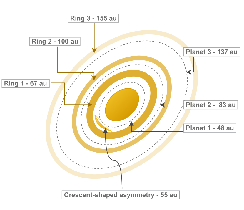
Figure 1: Sketch of the oberserved dust substructure of the HD 163296 system. The colored rings and the crescent-shaped feature mimic the dust while the grey dashed lines indicate the semi-major axes of the modeled planetary system. The labels introduced in this figure will be used throughout the text.

The origin of such a structure is unknown and a preliminary model was presented in Zhang et al. (2018) involving planet-disk interaction. In these models asymmetries in the co-orbital region are common if the viscosity is low.
Before the publication of the results from the DSHARP campaign, the HD 163296 disk was modeled by Liu et al. (2018). Their models incorporated 2D two-fluid hydrodynamical simulations with three planets in their respective positions matching the observed gaps. With synthetic images using radiative transfer calculations they could match the observed density profile with 0.46, 0.46, and 0.58 Jupiter masses for the three planets and a radially increasing turbulent viscosity parametrization.
In the suite of simulations by Zhang et al. (2018) using hydrodynamical models with Lagrangian particles the proposed mass fits are 0.71, 2.18, and 0.14 Jupiter masses for an $\alpha$-viscosity of $10^{-3}$. In their lower viscosity models of $\alpha=10^{-4}$ masses of 0.35, 1.07, and 0.07 Jupiter masses were fitted.
Further observational constraints of the hypothetical two outer planets were provided by kinematical detections by Teague et al. (2018). Their model predicts masses of 1 and 1.3 Jupiter masses for these planets. Pinte et al. (2020) argue that velocity ”kinks” observed in the CO observations with ALMA are evidence of nine planets in the DSHARP sample, including two planets in the HD 163296 disk at 86 au and 260 au. The signal-to-noise ratio is not sufficient to probe the inner gap at 48 au.
In this paper we want to further explore the possibility of reproducing the observed structures by planet-disk interaction with a focus on the crescent-shaped asymmetry in the dust emission. This asymmetric feature has been present in the works discussed above but it has not been subject to more detailed analysis yet. Given the motivation of the crescent-shaped feature in the observation of HD 163296 we aim to constrain the visibility of such an agglomeration of dust caused by planet-disk interaction and its dependence on the physical parameters of the system like planet mass, turbulent viscosity and dust size. In comparison to the study of Zhang et al. (2018) we employ two-dimensional hydrodynamical models with a fluid formulation of dust.
Sec. 2 introduces the physical model and code setup as well as the post processing pipeline to predict observable features. In Sec. 3 we present the main results of our study. Sec. 4 compares these findings with previous works and addresses limitations of the model. In Sec. 5 we summarize the main results with concluding remarks.

2 Model

All hydrodynamical models presented in this work were performed with the FARGO3D multi-fluid code (Benítez-Llambay & Masset, 2016; Benítez-Llambay et al., 2019) making use of an orbital advection algorithm (Masset, 2000). The code is based on the public version of FARGO3D with the addition of allowing a constant dust size throughout the simulation and a spatially variable viscosity.

2.1 Basic equations

The FARGO3D code solves the conservation of mass (Eqs. [1] and [3]) and conservation of momentum (Eqs. [2] and [4]) for gas and dust in our model setups:

$$\partial_{\mathrm{t}}\Sigma_{\mathrm{g}}+\nabla\cdot\left(\Sigma_{\mathrm{g}}\,\bm{v}_{\mathrm{g}}\right)=0$$ (1)

$$\Sigma_{\mathrm{g}}\left[\partial_{\mathrm{t}}\bm{v}_{\mathrm{g}}+\left(\bm{v}_{\mathrm{g}}\cdot\nabla\right)\bm{v}_{\mathrm{g}}\right]=-\nabla P+\nabla\cdot\Pi-\Sigma_{\mathrm{g}}\nabla\Phi-\sum_{\mathrm{i}}\Sigma_{\mathrm{i}}\mathrm{f}_{\mathrm{i}}$$ (2)

$$\partial_{\mathrm{t}}\Sigma_{\mathrm{d,i}}+\nabla\cdot\left(\Sigma_{\mathrm{d,i}}\,\bm{v}_{\mathrm{d,i}}+\bm{j}_{\mathrm{i}}\right)=0$$ (3)

$$\Sigma_{\mathrm{d,i}}\left[\partial_{\mathrm{t}}\bm{v}_{\mathrm{d,i}}+\left(\bm{v}_{\mathrm{d,i}}\cdot\nabla\right)\bm{v}_{\mathrm{d,i}}\right]=-\Sigma_{\mathrm{d,i}}\nabla\Phi+\Sigma_{\mathrm{d,i}}\mathrm{f}_{\mathrm{i}}$$ (4)

Here, $\Sigma_{\mathrm{g}}$ denotes the gas surface density, $\Sigma_{\mathrm{d},\mathrm{i}}$ the corresponding dust species, $P=\Sigma_{\mathrm{g}}c_{\mathrm{s}}^{2}$ the gas pressure, linked to the density by a locally isothermal equation of state with the sound speed $c_{\mathrm{s}}$, $\Phi$ the gravitational potential of the star and planets, $\Pi$ the viscous stress tensor, $f_{\mathrm{i}}$ the interaction forces between gas and dust and $\bm{v}_{\mathrm{g}}$ and $\bm{v}_{\mathrm{d},i}$ the gas and dust velocities respectively. Dust feedback is included by the term $\sum_{\mathrm{i}}\Sigma_{\mathrm{i}}f_{\mathrm{i}}$ in Eq. 2.
We consider turbulent mixing and diffusion of dust grains by using the dust diffusion implementation described in Weber et al. (2019). The corresponding diffusion flux $\bm{j}_{\mathrm{i}}$ can be written as

$$\bm{j}_{\mathrm{i}}=-D_{\mathrm{i}}\left(\Sigma_{\mathrm{g}}+\Sigma_{\mathrm{d},\mathrm{i}}\right)\nabla\left(\frac{\Sigma_{\mathrm{d},\mathrm{i}}}{\Sigma_{\mathrm{g}}+\Sigma_{\mathrm{d},\mathrm{i}}}\right),$$ (5)

with the diffusion constant $D_{\mathrm{i}}$ being proportional to the turbulent viscosity $\nu$ (Youdin & Lithwick, 2007):

$$D_{\mathrm{i}}=\nu\frac{1+\mathrm{St}_{\mathrm{i}}^{2}}{\left(1+\mathrm{St}_{\mathrm{i}}^{2}\right)^{2}}.$$ (6)

The Stokes number $\mathrm{St}_{\mathrm{i}}$ of dust species $\mathrm{i}$ is proportional to the stopping time $t_{\mathrm{stop}}$ and can be written as

$$\mathrm{St}_{\mathrm{i}}=t_{\mathrm{stop}}\,\Omega_{\mathrm{K}}=\frac{\pi}{2}\frac{a_{\mathrm{i}}\,\rho_{\mathrm{d}}}{\Sigma_{\mathrm{g}}},$$ (7)

where $\Omega_{\mathrm{K}}$ is the Keplerian angular frequency, $a_{\mathrm{i}}$ the dust grain size and $\rho_{\mathrm{d}}$ the material density of the grains. The gas-dust interaction is modeled using the Epstein drag law, which is expected to be valid if the particle size is smaller than the mean-free path of surrounding gas molecules. Here, the drag force is proportional to the relative velocities between the corresponding fluids (Whipple, 1972). The drag force $\bm{f}_{\mathrm{i}}$ can be expressed as

$$\bm{f}_{\mathrm{i}}=-\frac{\Omega_{\mathrm{K}}}{\mathrm{St}_{\mathrm{i}}}\left(\bm{v}_{\mathrm{d},\mathrm{i}}-\bm{v}_{\mathrm{g}}\right).$$ (8)

2.2 Disk model

In the disk model the planet-disk interaction is implemented as an additional smoothed potential term (Plummer-potential) for each planet. The smoothing length is set to $0.6H$, where $H(r)=c_{\mathrm{s}}(r)/\Omega_{\mathrm{K}}(r)$ is the pressure scale height at the radial distance $r$. The specific factor acts as a correction for 3D effects in the 2D simulation (Müller et al., 2012).
Three planets are modeled in the simulations. The two outer ones are set to the locations indicated by Teague et al. (2018). The inner planet is put at the corresponding gap location while the mass is varied in the different runs. In the fiducial models, the planet locations and masses are $r_{\mathrm{p}}=\{48,83,137\}$ au, $M_{\mathrm{p0}}=\{1.0,0.55,1.0\}\,M_{\mathrm{jup}}$, respectively. From this point on we will refer to the three planets as planet 1, 2 and 3. The same notation will be used for the apparent ring structures, i.e. ring 1: observed or modeled ring at 67 au; ring 2 at 100 au (see Fig. 1). We chose lower the mass of planet 2 compared to the one predicted in Teague et al. (2018) since it allows a sufficiently massive ring 2 while not significantly disturbing the crescent-shaped asymmetry by its repeated gravitational interaction.
For the fiducial model the corresponding parameter variations we set the planet mass $M_{\mathrm{p}}$ to its final value $M_{\mathrm{p0}}$ at the beginning of the simulation. The mass growth time scale however is known to have an impact on the formation of disk structures, such as vortices (Hammer et al., 2019; Hallam & Paardekooper, 2020). We therefore investigate the robustness of the results by testing different planet growth time scales:

$$M_{\mathrm{p}}(t)=\frac{1}{2}\left[1-\mathrm{cos}\left(\pi\frac{t}{T_{\mathrm{G}}}\right)\right]\,M_{\mathrm{p0}}$$ (9)

$T_{G}$ refers to the planet growth time scale ranging from $10T_{0}$ to $500T_{0}$ with $T_{0}$ denoting the orbital period at $r_{0}=48\leavevmode\nobreak\ \mathrm{au}$. By using this simplified growth prescription we do not directly model the accretion of gas onto the planets and we thus do not artificially remove any mass from the simulation domain. Furthermore, for all models the displacement of the center of mass by the influence of the planets is taken into account as an additional indirect term added to the potential. The semi-major axes of the planets are kept fixed throughout the whole simulation.
The initial surface density profile is assumed to be a power law with an exponential cutoff:

$$\Sigma_{\mathrm{g}/\mathrm{d}}=\Sigma_{\mathrm{g}/\mathrm{d},0}\left(\frac{r}{r_{0}}\right)^{-\mathrm{p}}\mathrm{exp}\left[-\left(\frac{r}{r_{0}}\right)^{\mathrm{s}}\right]\,,$$ (10)

with $r_{0}=48\,\text{au}$ and the initial gas and dust surface densities $\Sigma_{\mathrm{g},0}$ and $\Sigma_{\mathrm{d},0}$. Similar to the models of Liu et al. (2018) we choose a surface density slope of $\mathrm{p}=0.8$. For the dust a sharper cutoff of $\mathrm{s}=2$ was chosen compared to the gas cutoff of $\mathrm{s}=1$. In all simulation runs an initial dust-to-gas ratio of $\left(\sum_{\mathrm{i}}\Sigma_{\mathrm{d},\mathrm{i}}\right)/\Sigma_{\mathrm{g}}=0.01$ is assumed.
We approximate the disk thermodynamics with a locally isothermal equation of state. The model is parametrized through locally isothermal sound speed

$$c_{\mathrm{s}}=\frac{H(r_{0})}{r_{0}}\left(\frac{r}{r_{0}}\right)^{\frac{1}{4}}\,\Omega_{\mathrm{K}}r.$$ (11)

This corresponds to a flared disk with flaring index 0.25. The aspect ratio $H/r$ at $r_{0}$ is set to a value of 0.05. Assuming a mean molecular weight of $\mu=2.353$ the mid plane temperature profile can be written in the following way

$$T_{\mathrm{mid}}(r)=\sqrt{\frac{\mu m_{\mathrm{p}}}{k_{\mathrm{B}}}}\,c_{\mathrm{s}}\approx 25\,\left(\frac{r}{r_{0}}\right)^{-\frac{1}{2}}\mathrm{K},$$ (12)

with the proton mass $m_{\mathrm{p}}$. The temperature at 48 au matches the findings of Dullemond et al. (2019).
We assume a radially smoothly increasing turbulent viscosity profile, motivated by Eq. 4 in the work of Liu et al. (2018) and similar dead zone parametrizations presented in Pinilla et al. (2016) and Miranda et al. (2016):

$$\alpha(r)=\alpha_{\mathrm{min}}\left\{1-\frac{1}{2}\left(1-\frac{\alpha_{\mathrm{max}}}{\alpha_{\mathrm{min}}}\right)\left[1-\mathrm{tanh}\left(-\frac{r-R}{\sigma r_{0}}\right)\right]\right\},$$ (13)

where the parameters $R$ and $\sigma$ are set to 144 au and 1.25 respectively. Similar to the values in Liu et al. (2018) the parameter $R$ refers to the mid-point of the transition in $\alpha$ whereas $\sigma$ defines the slope.

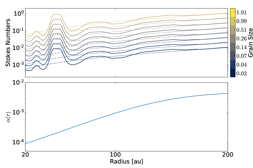
Figure 2: Upper panel: azimuthally averaged values of the Stokes number St of model fid. The dashed lines indicate the initial values and the solid lines represent the state after $500\,T_{0}$.
Lower panel: prescribed $\alpha$ viscosity. The blue line visualizes the radially increasing $\alpha$ viscosity set in the model.

2.3 Boundary conditions

The radial velocities in the ghost cells are set according to anti-symmetric boundary conditions. On a staggered mesh this corresponds to $v_{\mathrm{r}}(r_{\mathrm{ghost}})=-v_{\mathrm{r}}(r_{\mathrm{act}})$, where $r_{\mathrm{ghost}}$ is the ghost cell and $r_{act}$ the equivalent mirrored cell on the active hydro mesh near the boundary. The value at the staggered boundary itself is set to zero. The azimuthal velocities are set to the initial Keplerian profile in the ghost zone.
The surface density is extrapolated according to the density gradient exponent p. Additionally, wave damping is applied within 15% of the respective boundary radius. In this region the density is exponentially relaxed towards the initial values within 0.3 local orbital time scales. The procedure follows the wave damping boundary conditions used in de Val-Borro et al. (2006).
We tested the robustness of the wave damping with respect to the chosen inner boundary condition. No significant wave reflections are detected for both a symmetric and anti-symmetric inner boundary condition. The relative difference between these two approaches is on the order of $10^{-5}$ compared to the reflected perturbations of $\approx 10^{-2}$ without wave damping.

2.4 Code setup and parameters

Various ranges of individual disk parameters were considered for constraining the impact onto dust features in the simulations. Table 1 gives an overview over the performed simulations and their parameter choices.
For most of the runs a resolution of 560 radial and 895 azimuthal cells was chosen where the grid is logarithmically spaced in radial direction. Compared to the local disk scale height a ratio of roughly 7 cells per scale height is achieved in each direction. The models with the suffix _dres were run with a resolution of 14 cells per scale height. The low resolution runs are subject to a larger numerical diffusion compared to the high resolution models. Although these runs can be used for mass estimates of the crescent-shaped feature, the results should be taken with caution concerning the dust substructure lifetime. Whenever this difference becomes significant we default to the high resolution runs. Further details are given in appendix B. For all simulations the mass of the central star is set to $1.9\,M_{\odot}$ The parameters $\alpha_{\mathrm{min}}$ and $\alpha_{\mathrm{max}}$ are set to $10^{-5}$ and $5\cdot 10^{-3}$ which results in a value of $\alpha(r_{0})\approx 2\cdot 10^{-4}$ at the location of $r_{0}=48\,\mathrm{au}$. The radial profile of $\alpha(r)$ is shown in the lower panel of Fig. 2.
The dust is sampled by 8 separate fluids with Stokes numbers spaced logarithmically ranging from $1.3\cdot 10^{-3}$ to $1.3\cdot 10^{-1}$ at $r_{0}=48\,\mathrm{au}$. In the code, the equivalent grain size at $r_{0}$ is applied to the whole domain and is kept constant throughout the whole simulation. With an initial value of $\Sigma_{\mathrm{g},0}=37.4\,\mathrm{g}/\mathrm{cm}^{2}$ the minimum and maximum grain sizes are $a_{\mathrm{min}}=0.19\,\mathrm{mm}$ and $a_{\mathrm{max}}=19\,\mathrm{mm}$. No dust size evolution is modeled here. It should be noted that these state the initial values of St and changes with time depending on the gas surface density, as shown in the upper panel of Fig. 2. The most prominent change of an increase of about one order of magnitude in St occurs at the gap carved by planet 1 after 500 orbits.
The majority of models neglects dust feedback to the motion of the gas. Each dust species can thus be scaled in density individually without violating the validity of the dynamical features.
Per default, the simulations are executed until $1000\,T_{0}$. Simulation runs with a nonzero growth time scale $T_{\mathrm{G}}$ and the model fid_dres are run until $2000\,T_{0}$. After $\approx 900$ orbits the gas and dust structure converges. The crescent-shaped asymmetry builds up to a stable niveau after less than 100 orbits. We refer to Sec. 3 for more details.

Table 1: Relevant simulation runs and their respective numerical parameters.

Simulation	H/r	$M_{\mathrm{pl1}}$ [$M_{\mathrm{jup}}$]	$M_{\mathrm{pl2}}$ [$M_{\mathrm{jup}}$]	$e$	$N_{r}$	$N_{\phi}$	$r_{\mathrm{cut}}$ [au]	$\alpha$	$T_{\mathrm{G}}$
fid	0.05	1	0.55		560	895		$2\cdot 10^{-4}$	0
fid_dres	0.05	1	0.55		1120	1790		$2\cdot 10^{-4}$
hr4	0.04
hr45	0.045
hr55	0.055
hr6	0.06
taper10									10
taper50									50
taper100									100
taper500									500
p1m1		0.20
p1m2		0.36
p1m3		0.52
p1m4		0.68
p1m5		0.84
p1m1fb		0.20
p1m2fb		0.36
p1m3fb		0.52
p1m4fb		0.68
p1m5fb		0.84
p1m6fb
p1m6fb_dres					1120	1790
p2m1			0.30
p2m2			0.42
p2m3			0.54
p2m4			0.66
p2m5			0.78
p2m6			0.90
ecc1				0.02
ecc2				0.04
ecc3				0.06
ecc4				0.08
ecc5				0.10
cut1							150
cut2							175
cut3							200
cut4							225
cut5							250
alpha1								$1\cdot 10^{-5}$
alpha1_dres					1120	1790		$1\cdot 10^{-5}$
alpha2								$1\cdot 10^{-4}$
alpha3								$5\cdot 10^{-4}$
alpha3_dres					1120	1790		$5\cdot 10^{-4}$
alpha4								$1\cdot 10^{-3}$
alpha4_dres					1120	1790		$1\cdot 10^{-3}$
alpha5								$2\cdot 10^{-3}$
alpha6								$3\cdot 10^{-3}$
alpha6_dres					1120	1790		$3\cdot 10^{-3}$

Table 2: Optical depth fitting results for ring 1.

Constant	$\Sigma_{\mathrm{g},0}\,(r=48\,\mathrm{au})$ [$\frac{g}{cm^{2}}$]	$\Sigma_{\mathrm{g},0}\,(r=1\,\mathrm{au})$ [$\frac{g}{cm^{2}}$]	$a_{\mathrm{min}}$ [mm]	$a_{\mathrm{max}}$ [mm]	$\kappa_{\mathrm{min}}$ [$\frac{cm^{2}}{g}$]	$\kappa_{\mathrm{max}}$ [$\frac{cm^{2}}{g}$]
Grain size	37.4	827.7	0.191	19.1	1.32	0.11
d/g ratio	1.31	28.91	0.007	0.67	0.40	3.30

Table 3: Gaussian fit results of the simulated dust rings for all Stokes numbers, $\mathrm{St}$.

a [mm]	St	$w_{\mathrm{ring1}}$ [au]	$w_{\mathrm{ring2}}$ [au]	$r_{\mathrm{ring1}}$ [au]	$r_{\mathrm{ring2}}$ [au]	$M_{\mathrm{ring1}}$ [$M_{\mathrm{earth}}$]	$M_{\mathrm{ring2}}$ [$M_{\mathrm{earth}}$]
0.2	$1.3\cdot 10^{-3}$	$4.09\pm 0.09$	$10.5\pm 0.17$	$62.26\pm 0.09$	$100.18\pm 0.16$	2.1	1.9
0.4	$2.6\cdot 10^{-3}$	$3.13\pm 0.08$	$7.10\pm 0.09$	$62.05\pm 0.08$	$99.90\pm 0.09$	2.9	2.9
0.7	$5.0\cdot 10^{-3}$	$2.27\pm 0.07$	$4.80\pm 0.04$	$61.90\pm 0.07$	$99.25\pm 0.04$	4.0	4.7
1.4	$9.6\cdot 10^{-3}$	$1.68\pm 0.05$	$3.34\pm 0.01$	$61.86\pm 0.05$	$98.87\pm 0.01$	5.5	8.0
2.6	$1.9\cdot 10^{-2}$	$1.28\pm 0.04$	$2.37\pm 0.01$	$61.89\pm 0.04$	$98.69\pm 0.01$	7.9	12.3
5.1	$3.6\cdot 10^{-2}$	$1.00\pm 0.03$	$1.76\pm 0.01$	$61.92\pm 0.03$	$98.67\pm 0.01$	11.5	17.0
9.9	$6.9\cdot 10^{-2}$	$0.80\pm 0.03$	$1.33\pm 0.01$	$61.93\pm 0.03$	$98.67\pm 0.01$	17.3	22.2
19.1	$1.3\cdot 10^{-1}$	$0.64\pm 0.02$	$1.01\pm 0.01$	$61.94\pm 0.02$	$98.66\pm 0.01$	28.0	26.9
sum (high mass model)						79.3	95.9
sum (low mass model)						11.4	13.8

2.5 Radiative transfer model and post processing

In order to compare the results of the hydrodynamical simulations with the observational data synthetic images are produced with RADMC-3D (Dullemond et al., 2012) and the CASA package (McMullin et al., 2007). The results of the hydrodynamical simulations have to be extended to three dimensional dust density models which then serve as input for the radiative transfer calculations with RADMC-3D.
Using the given Stokes numbers of the hydro model, the respective dust sizes are computed via Eq. 7. The number density size distribution of the dust grains follows the MRN distribution $n(a)\propto a^{-3.5}$ (Mathis et al., 1977) where a is the grain size.
Dust settling towards the mid-plane is considered following the diffusion model of Dubrulle et al. (1995)

$$H_{\mathrm{d}}=\sqrt{\frac{\alpha}{\alpha+\mathrm{St}}}H$$ (14)

Here, we assume a Schmidt number on the order of unity. The grid resolution for the radiative transfer is identical to the hydrodynamical mesh. In polar direction the grid is expanded by 32 cells which are equally spaced up to $z_{\mathrm{lim}}=\pi/2\pm 0.3$. The vertical disk density profile is assumed to be isothermal and the conversion from the surface density to the local volume density is calculated as follows:

$$\rho_{\mathrm{cell}}=\frac{\Sigma}{\sqrt{2\pi}H_{\mathrm{d}}}\cdot\mathrm{erf}^{-1}\left(\frac{z_{\mathrm{lim}}}{\sqrt{2}H_{\mathrm{d}}}\right)\cdot\frac{\pi}{2}H_{\mathrm{d}}\frac{\ \left[\mathrm{erf}\left(\frac{z_{+}}{\sqrt{2}H_{\mathrm{d}}}\right)-\mathrm{erf}\left(\frac{z_{-}}{\sqrt{2}H_{\mathrm{d}}}\right)\right]}{z_{+}-z_{-}}.$$ (15)

The error function term is a correction for the limited domain extend in the vertical direction that would otherwise lead to an underestimation of the total dust mass. Similarly, the second correction term accounts for the finite vertical resolution, especially important for thin dust layers with strong settling towards the mid-plane. The coordinates $z_{+}$ and $z_{-}$ denote the cell interface locations in polar direction along the numerical grid.
For each grain size bin and a wavelength of 1.3 mm the corresponding dust opacities were taken from the dsharp_opac package which provides the opacities presented in Birnstiel et al. (2018). These opacities are based on a mixture of water ice, silicate, troilite and refractory organic material. The grains are assumed to be spherically shaped and to have no porosity. In the RADMC-3D model, the central star is assumed to have a mass of 1.9 solar masses with an effective temperature of 9333 K which results in a luminosity of $2.62\cdot 10^{34}\mathrm{erg}/\mathrm{s}$. The system is assumed to be at a distance of 101 pc. For the dust temperature calculation a number of $n_{\mathrm{phot}}=10^{8}$ photon packages and for the image reconstruction $n_{\mathrm{phot\_scat}}=10^{7}$ photon packages were used. The thermal Monte-Carlo method is based on the recipe of Bjorkman & Wood (2001). We include isotropic scattering in the radiative transfer calculation. A comparison between the prescribed gas temperatures and the computed dust temperatures is given in Appendix D.
For simulating the detectability of the various features present in the model we use the task simalma from the CASA-5.6.1 software. A combination of the antenna configurations alma.cycle4.8 and alma.cycle4.5 was chosen. The simulated observation time for configuration 8 is 2 hours while the more compact configuration is integrated over a reduced time with a factor of 0.22 corresponding 0.44 hours.
We employed the same cleaning procedure as made available in Isella et al. (2018) to reduce the artificial features from the incomplete uv-coverage and to allow a comparison to the observation. The procedure involves the CASA task tclean with a robust parameter of -0.5 and manual masking of the disk geometry. Consistent with the radiative transfer model, the observed wavelength is simulated to be at $1.3\,\mathrm{mm}$, corresponding to ALMA band 6.

3 Results

In the following parts the outcome of the simulation runs listed in Table 1 will be presented and analyzed. First, the variety of substructures emerging from the interaction of gas, dust and the three planets will be described. Afterwards parameter dependence and observability will be addressed.

3.1 Dust substructure overview

A variety of dust substructures emerges from the planet-disk system during its dynamical evolution. Fig. 3 and Fig. 4 show the dust surface density structure for a selected parameter space of aspect ratio and the turbulent viscosity, characterized by $\alpha$. In the following analysis of the crescent-shaped asymmetries simulation snapshots after 500 orbits at 48 au are compared with each other since their evolution is comparable for all resolutions. Most prominently multiple rings form in most cases. As expected, fluids with larger Stokes numbers $\mathrm{St}$ and thus larger grain sizes exhibit thinner rings and more concentrated substructures. Especially, nonaxisymmetric features can be seen mostly for $a\geq 2.6\,\mathrm{mm}$ or $\mathrm{St}>10^{-2}$. For smaller dust sizes the dust is better coupled to the gas and resembles its structure more closely.
Additionally, if a crescent-shaped asymmetry is present, it is situated in the gap caused by the most inner planet at 48 au for the majority of the parameter space. Further asymmetries appear if the $\alpha$-viscosity is radially constant with values of $\alpha\leq 1\cdot 10^{-3}$ or for low values of the aspect ratio $h$. Dust is preferably trapped in the Lagrange point L5. In Fig. 3 rings and asymmetries become weaker with increasing aspect ratio. A crescent-shaped feature at the L5 position is present for all aspect ratios while a second similar asymmetry at the L4 point appears for values of H / r ¡ 0.05. The crescent weakens for smaller grain sizes. Also the second prominent ring beyond planet 2 at 83 au weakens clearly for larger aspect ratios. In the combination of the largest grain sizes and $H/r$ the ring completely vanishes.
To highlight the importance of the turbulent $\alpha$ viscosity parameter a subset of results with radially constant values of $\alpha$ are shown in Fig. 4. Not surprisingly, larger values of alpha generally lead to a more diffuse and symmetric distribution of dust. Below $\alpha=5\cdot 10^{-4}$ no concentric rings form due to vortices in the gas. Crescent-shaped features in both Lagrange points of the innermost planet are visible in the very low viscosity case of $\alpha=10^{-5}$. A sufficiently large viscosity on the other hand also leads to the disappearance of the second ring in the limit of larger grains and Stokes numbers, similar to the large aspect ratio in Fig. 3. The collection of these results also stresses the issue with a radially constant $\alpha$ viscosity with respect to the observed HD 163296 system. In order to reproduce a nonaxisymmetric feature in the vicinity of the inner planet and a smooth ring-shaped outer structure, a radially increasing value of $\alpha$ would be the natural choice. This is also consistent with an embedded dead zone at the inner part of the disk and a more active outer disk region with a higher degree of ionization (Miranda et al., 2016; Pinilla et al., 2016). We thus chose a radially increasing $\alpha$ viscosity for all remaining simulation runs.
Models with a variation in the dust cutoff radius only show little changes in the resulting dust structures. Only this subset of the possible parameter space already exposes the degeneracy of the emerging substructures with respect to the chosen disk models.

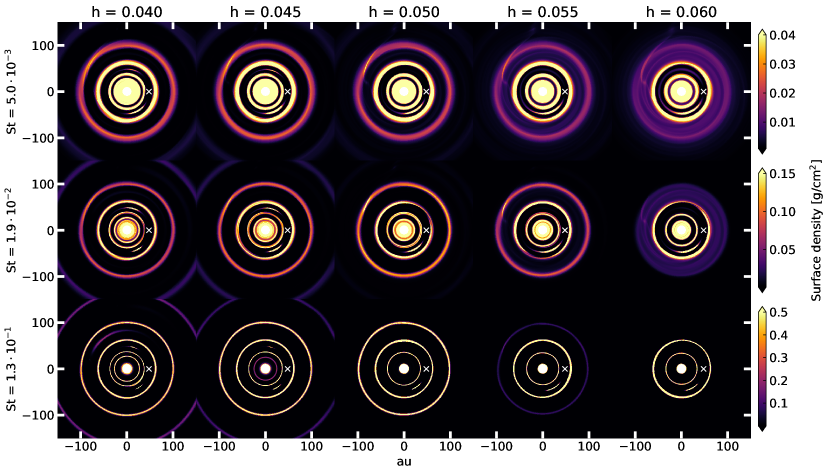
Figure 3: Shown are dust surface density maps for a subset of three fluids with varying values of the aspect ratio $h=H/r$ at 500 orbits at 48 au. Crescent-shaped asymmetries are visible for all aspect ratios. Large values of $h$ weaken dust accumulation in the co-orbital regions of the planets. The white crosses mark the position of planet 1.

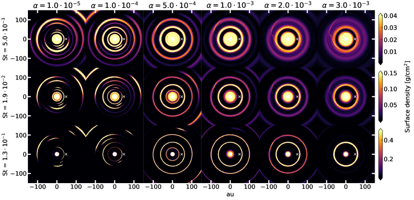
Figure 4: Dust surface density maps for different values of a radially constant $\alpha$ viscosity after 500 orbits at 48 au. For $\alpha\leq 10^{-4}$ strong asymmetries are present. ring 2 weakens or vanishes for large viscosities. The white crosses mark the position of planet 1.

3.2 Rings

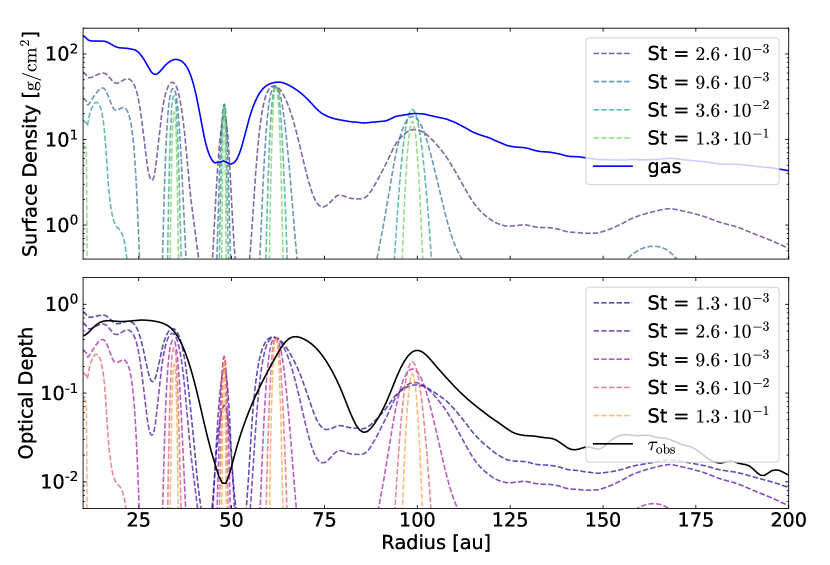
Figure 5: Upper panel: azimuthally averaged dust and gas surface densities of model fid_dres after 1000 orbits at 48 au. Dust density profiles are normalized to the gas peak value at the location of ring 1.
Lower panel: azimuthally averaged optical depths of model mid after 1000 orbits at 48 au compared to the observed optical depth $\tau_{\mathrm{obs}}$. Simulated optical depths are normalized to $\tau_{\mathrm{obs}}$ at the location of ring 1.

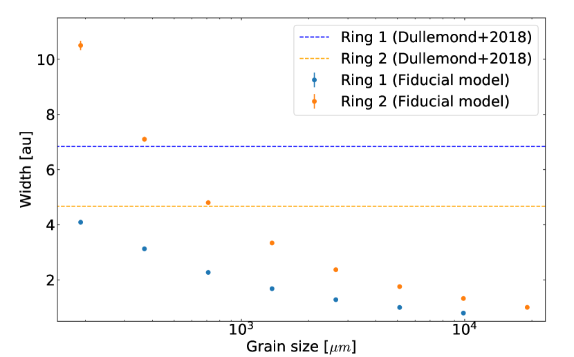
Figure 6: Ring widths of model fid_dres after 1000 orbits at 48 au. Simulated values are compared to the inferred ring widths of Dullemond et al. (2018), displayed as the horizontal dashed lines.

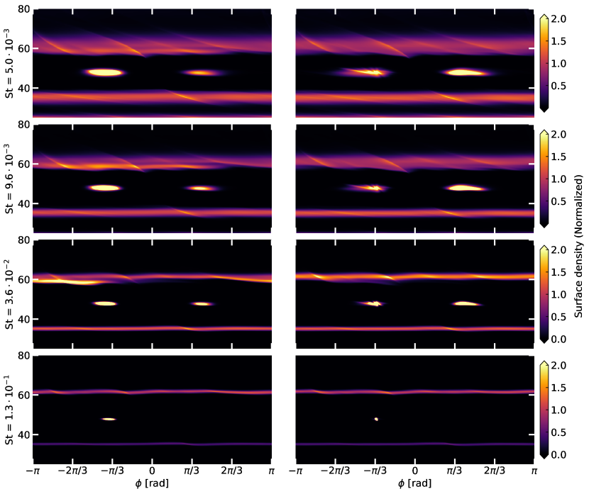
Figure 7: Dust surface density maps in polar coordinates for model fid_dres without dust feedback (left hand side) and p1m6fb_dres with dust feedback after 500 orbits at 48 au for four different initial Stokes numbers and dust sizes. A dust agglomeration around the location of the trailing Lagrange point L5 is present for all Stokes numbers. Unlike the nonfeedback case the right panels show that dust is trapped more efficiently in the leading Lagrange point L4 for smaller Stokes numbers. For $\mathrm{St}\lesssim 3.6\cdot 10^{-2}$ the L4 feature is more pronounced than the dust over density around L5. Dust feedback leads to an instability at the L5 point and fragments the asymmetric feature. Dust densities are normalized to the peak value of ring 1.

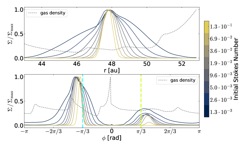
Figure 8: Radial and azimuthal cut through the maximum of the crescent-shaped asymmetry around L5 of the fiducial model fid_dres after 500 orbits at 48 au. The color map indicates the different initial Stokes numbers of the dust fluids. The dashed lines represent the gas density. The surface densities are normalized to their respective maximum value in the co-orbital region of planet 1. The light blue and light green vertical lines indicate the Lagrange points L5 and L4 respectively.

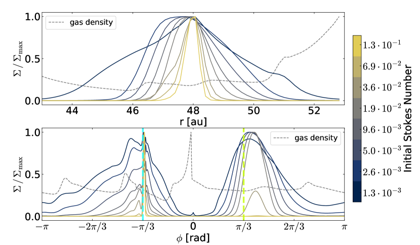
Figure 9: Radial and azimuthal cut through the maximum density value in the co-orbital region of the model p1m6fb_dres with dust feedback after 500 orbits at 48 au. The light blue and light green vertical lines indicate the Lagrange points L5 and L4 respectively. Depending on the location of the feature the density cuts are normalized to the peak value in the region of L4 or L5. Smaller dust with $\mathrm{St}\lesssim 3.6\cdot 10^{-2}$ preferably concentrates in L4.

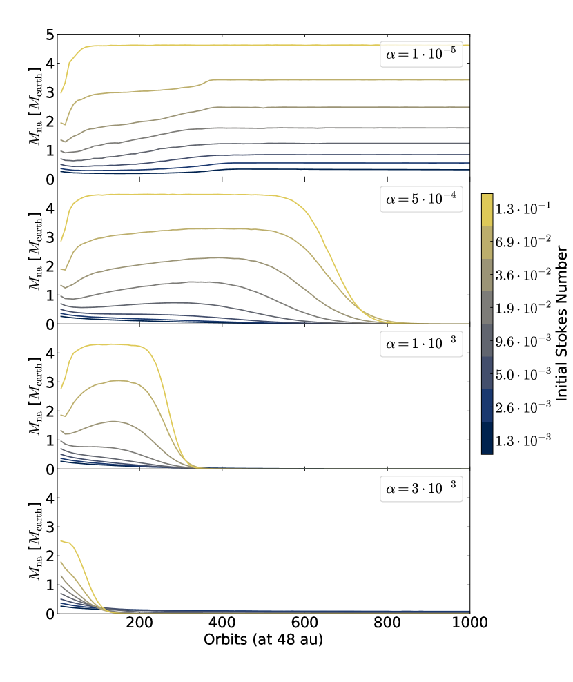
Figure 10: Development of the trapped dust mass in the L5 region for different $\alpha$ viscosities over time with a resolution of 14 cells per scale height. Dust masses $M_{\mathrm{na}}$ in the nonaxisymmetric feature denoted are integrated down to a cut-off value of $10^{-2}\,\Sigma_{\mathrm{max}}$ and normalized to the high mass model stated in Table 2.

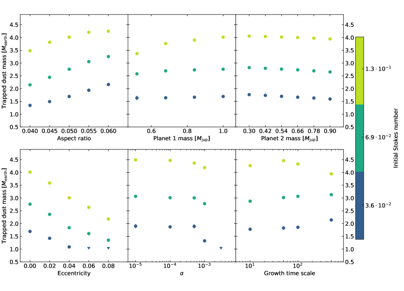
Figure 11: Trapped dust masses in earth masses in the L5 feature for the largest three inital Stokes numbers. The mass values are averaged over the approximately constant mass time frame starting from $100\,T_{0}$. Dust masses are normalized according to the high mass model stated in Table 2. Missing data points are equivalent to a nonexistence of a stable crescent-shaped asymmetry in the co-orbital region around 48 au.

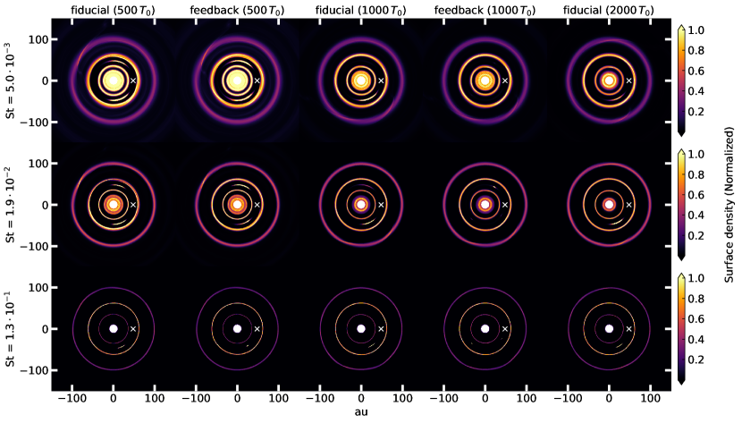
Figure 12: Comparison of the dust surface density map for three different dust sizes of the models fid_dres (fiducial) and p1m6fb_dres (feedback) at different simulation times. The surface densities are normalized to the peak value at ring 1.

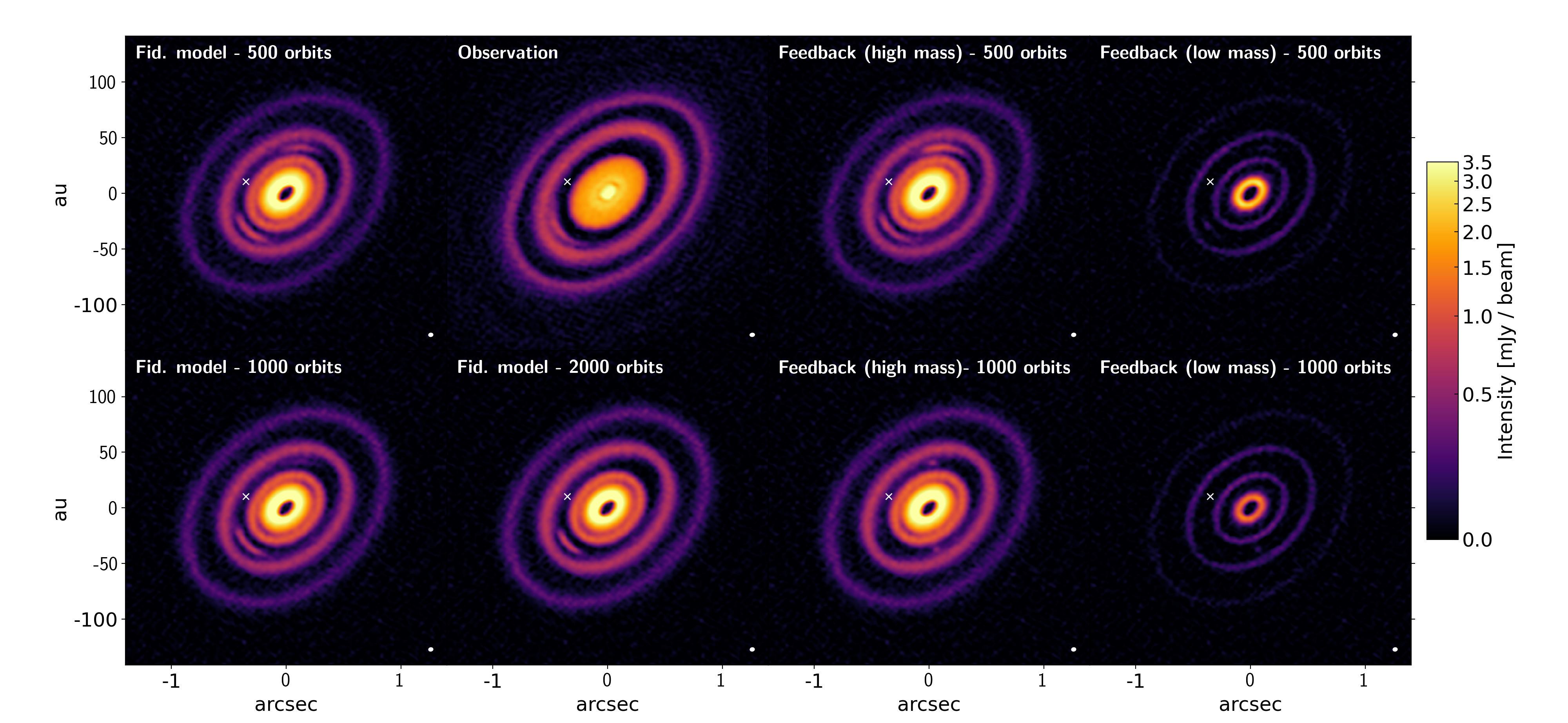
Figure 13: Comparison of the synthetic images based on the models fid_dres (first and second column), p1m6fb_dres (third and fourth column) with the observation taken from Andrews et al. (2018); Isella et al. (2018). The ellipsis at the lower right of each panel visualizes the synthesized beam. The beam size is $49.7\times 41.4\,\mathrm{mas}$ for the synthetic images. The rms noise reaches $\approx 50\,\mu\mathrm{as}$. The synthetic images are projected with an inclination of $46.7\degree$ and a position angle of $133.33\degree$.

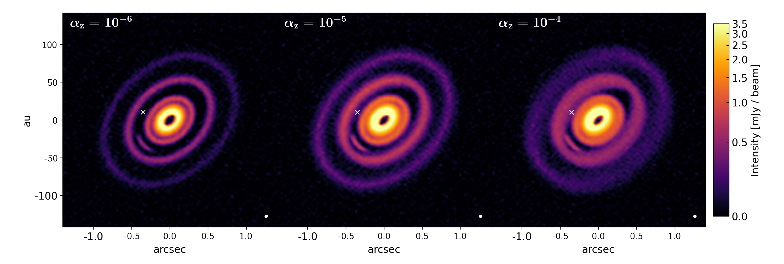
Figure 14: Comparison of the synthetic images based on the model fid_dres after 2000 orbits at 48 au with respect to the vertical dust mixing parametrized by $\alpha_{\mathrm{z}}$.

Before quantifying the nonaxisymmetric feature in the model, we want to compare properties of the ring structures with previous works and the observations. The general procedure is to azimuthally average the dust density maps after 1000 orbits at 48 au and to invoke Gaussian fitting of the dust rings, comparable to Dullemond et al. (2018). Since the ring structure is approximately converged after 900 orbits the following procedure is based on the snapshots at 1000 orbits.
Fig. 5 shows the results of the high resolution fiducial model fid_dres as an example of the radial surface density structure. The increased resolution was chosen since the lower resolution models may overestimate the ring width and the trapped dust mass due to numerical diffusion (appendix B). In the upper panel the dust species is rescaled to gas density peak of ring 1. The dust rings are clearly thinner than the gaseous envelope and the ring width decreases with increasing dust grain sizes due to the stronger drift.
With the corresponding opacities $\kappa_{\mathrm{i}}$ a rough estimate of the resulting optical depth can be computed by $\tau_{\mathrm{sim}}=\kappa_{\mathrm{i}}\Sigma_{\mathrm{i}}$, where i denotes the dust species index. The results of this estimate are displayed in the lower panel of Fig. 5. All optical depths are rescaled to the values at the position of ring 1 from the profile $\tau_{\mathrm{obs}}$ derived in Huang et al. (2018). The profile provided in their work excludes contributions from the prominent nonaxisymmetric structures. Several properties become apparent:

• Ring 1 is wider than in the simulated profile.

• The peak location of ring 1 is located further outward with respect to the simulated one.

• The peak value of the optical depth of ring 2 from smaller grains and Stokes numbers is lower in the simulations compared to the estimated value from the observation.

A partial explanation of these differences could be that the dust-to-gas ratio could become larger than in the models so that dust feedback shifts the ring further outward and spreads the ring as shown in Weber et al. (2018) and Kanagawa et al. (2018). Here, the dust-to-gas ratio is not sufficient to cause a significant effect in the models including dust feedback.
A conclusion of Dullemond et al. (2018) was that the optical depth observed in the DSHARP survey were remarkably close to unity and that the rings were optically thin. Later Zhu et al. (2019) argued that dust scattering could account for this phenomenon and that the actual optical depth could be larger. In the case of HD 163296 the mass hidden in ring 1 could be thus larger than expected.
For ring fitting we use a Gaussian:

$$\Sigma_{\mathrm{fit}}(r)=A\,\mathrm{exp}\left(-\frac{(r-r_{0})^{2}}{2w}\right)$$ (16)

with the peak value $A$, the ring location $r_{0}$ and the ring width $w$. In Fig. 6 the fitted ring widths from model fid are plotted and compared to the observed values in Dullemond et al. (2018). Grain sizes of the high mass model are used. The width of ring 2 is matched close to a grain size of $1\,\mathrm{mm}$. On the other hand, the width of ring 1 is not reached with the parameters chosen in our models. It should be noted that the gas ring width is about 8 au, just slightly larger than the observed value of about 7 au. Smaller Stokes numbers could in principle reproduce these findings.
The equivalent model p1m6fb_dres including dust feedback shows no significant differences.

3.3 Surface density estimation

With ring 1 being the most prominent substructure in the observed system, its estimated lower bound for the surface density would be a reasonable choice for rescaling the simulated dust density maps. Furthermore, the crescent-shaped feature of interest is located closely to ring 1. In order to estimate a minimum mass of trapped dust in this feature an appropriate normalization of the density with respect to ring 1 would be a natural choice.
There are two possible methods in achieving a simple normalization. First, we rescale the sum of all azimuthally averaged dust densities so that the combined optical depth at the location of ring 1 equals the observed value. To maintain the validity of the dynamics of the system, the Stokes number corresponding to the grain size of a fluid has to be unmodified by this process. The immediate consequence is then a change in the dust-to-gas ratio if the densities are rescaled, since a change in the gas surface density with a constant grain size would modify the Stokes number (see Eq. 7). With a change in the dust-to-gas ratio the dust dynamics only remain comparable if no dust feedback is considered.
The second choice would be to maintain an initial dust-to-gas ratio of 0.01 and to change the dust grain size and the gas surface density. A modification of the grain size affects in turn the dust opacities and thus the optical depth. Consequently, the process of generating $\tau_{\mathrm{sim}}$, rescaling it to $\tau_{\mathrm{obs}}$ and inferring the corrected dust surface densities has to be iterated until convergence is achieved. Keeping the dust-to-gas ratio constant is important for the model runs with dust feedback enabled.
Table 2 provides relevant results from these two approaches which will be denoted by the high and low mass model in the following parts. With the unchanged grain sizes the dust-to-gas ratio diminishes to $\approx 2.4\cdot 10^{-3}$. For the iterative approach with the dust-to-gas ratio unchanged, the grain size distribution shifts towards smaller grains with a maximum size $a_{\mathrm{max}}\approx 0.67\,\mathrm{mm}$ and a minimum size $a_{\mathrm{min}}=0.007\,\mathrm{mm}$.
Results of the Gaussian fits onto the dust rings of the fiducial model are listed in Table 3 for all simulated dust species. The inferred ring widths are decreasing with increasing grain sizes and Stokes numbers. The peak maxima shift towards the star for larger grain sizes since the dust drift becomes more dominant in this regime. The total dust mass of all species is computed for both the low and high mass model. Dullemond et al. (2018) found masses of $56\,M_{\mathrm{earth}}$ and $43.6\,M_{\mathrm{earth}}$ for ring 1 and ring 2 respectively while assuming 1 mm grains with equal opacities values as used in the model presented here. The results of both the low and high mass model encompass the values of Dullemond et al. (2018).
The high mass model will be the preferred choice in the following diagrams and analysis since the opacity is dominated by smaller grain sizes compared to the low mass model. The choice is motivated by the broad ring structures apparent in the observations.

3.4 Secondary planet mass

In the models p2m1 - p2m6 the mass of the secondary planet at 83 au is varied in order to verify its impact on the ring structure. The results of Teague et al. (2018) indicate a planet mass of $1\,M_{\mathrm{jup}}$ within an error margin of $50\%$.
In our model runs we chose a mass of $0.55\,M_{\mathrm{jup}}$ for planet 2 since a larger mass causes a stronger dissipation of the crescent-shaped asymmetry. Lower masses significantly decreased the dust content in ring 2 and thus the fiducial planet mass value was chosen as the sweet spot between a strong ring contrast and an maximized asymmetric dust accumulation. Further details are given in appendix A.

3.5 Asymmetries

Of particular interest is the crescent-shaped asymmetry in the vicinity of ring 1 in HD 163296. Such a feature arises naturally in planet-disk interaction models including dust in the form of dust trapping in a Lagrange point of the gap carving planet. In this case planet 1 is responsible for dust trapping in the trailing L5 point which is also visible in Fig. 3 and Fig. 4 for a significant subset of the parameter space. An equivalent result was presented in Isella et al. (2018). In the following subsections we aim to perform a more extensive analysis of this feature in order to constrain physical properties of the dynamical system.

3.5.1 Structure & dust feedback

In Fig. 7 in the left panels dust surface density maps are shown in polar coordinates for four different dust fluids of model fid_dres. The region is focused around the co-orbital region of planet 1. Clearly, dust is concentrated in the trailing Lagrange point L5 of the Jupiter mass planet at 48 au. Several trends become apparent: Not surprisingly, dust grains are trapped more efficiently for larger grain sizes and Stokes numbers due to the stronger drift. Furthermore, the shape is more elongated for smaller Stokes numbers.
Does the dynamics of this feature change with the consideration of a dust back-reaction onto the gas? An example of the impact from dust feedback (model p1m1fb_dres) is given in Fig. 7 on the right hand side with the same parameters as model fid_dres. The crescent-shaped feature exhibits different structures compared to model fid_dres at the location of L5. The dust back-reaction onto the gas triggers and instability leading to fragmentation of the dust feature. Unlike the fiducial model, the additional crescent in the leading Lagrange point L4 of planet 1 is more pronounced than the L5 feature for smaller grain sizes and Stokes numbers. In the explored parameter space dust is significantly trapped for small aspect ratios or very low values of $\alpha<10^{-4}$ without the modeling of dust feedback. With the fiducial set of parameters the L4 feature slowly dissipates after more than a 1000 orbits.
A closer look on the radial and azimuthal extent of these dust shapes is provided in Fig. 8 for all simulated dust fluids. The surface densities of the crescent-shaped asymmetry are normalized to its maximum value. The radial and azimuthal width increases with decreasing values of the Stokes number. In the lower panel the density peak at the trailing L5 dominates the leading peak at L4 for all dust species. For smaller Stokes numbers and grain sizes the density maximum moves away from the planet location similar to the peak shift of the concentric dust rings described in Sec. 3.2.
In Fig. 9 we display the results of model p1m6fb_dres. Contrary to the nonfeedback case the density peak at L4 becomes significant for $\mathrm{St}\leq 3.6\cdot 10^{-2}$. In the vicinity of the L5 point two density peaks appear due to the fragmentation by dust feedback.
The azimuthal gas density profile reveals the momentary location of the spiral wakes caused by the planets as well as the gas accumulation around planet 1 itself at $\phi=0$.

3.5.2 Dynamical stability

In principle the crescent-shaped features in the co-orbital region are subject to diffusive processes like dust diffusion due to turbulent mixing or gravitational interaction with the planetary system (e.g. eccentric orbits). The dust trapping mechanism has to counteract these disruptive forces for the feature to be dynamically stable.
Fig. 10 corroborates this line of argument. The stability of the L5 feature is sensitive to the local value of the $\alpha$ viscosity. Given a value of $\alpha=10^{-5}$ the feature remains stable throughout almost the entirety of the simulation whereas $\alpha=10^{-3}$ shortens the existence down to about 300 dynamical time scales. For larger viscosities no discernable feature develops and the co-orbital region simply empties its dust content from the initial condition.
Studying the results of the models p1m1 to p1m5 we find that below about 0.4 to 0.5 Jupiter masses for planet 1 no stable feature forms since the gravitational interaction is not sufficient to enforce dust trapping in the Lagrange points. Qualitatively the feature life time is thus very sensitive to the given physical parameters. It should be noted that the absolute value in dynamical time scales could be underestimated due to the numerical diffusion present in the lower resolution runs. This additional diffusive effect prevents a stable trapping region around L4 and L5. Further details are provided in appendix B. In Fig. 10 we therefore plotted results with 14 cells per scale height.

3.5.3 Dust mass

A substantial amount of dust can be trapped in the feature at L5. The total mass ranges from roughly $1\,M_{\mathrm{earth}}$ for the low mass model to $10-15\,M_{\mathrm{earth}}$ for the high mass model. An overview of relevant parameters and their impact on the trapped dust mass is given in Fig. 11. Generally, if a sufficiently stable crescent-shaped asymmetry develops, the order of magnitude of the trapped dust mass is comparable for all parameters. Here, we only consider the three largest dust species since smaller grains are prone to be weakly trapped.
Only the low resolution simulations are compared to each other in this parameter study. The mass of the crescent-shaped feature was averaged over 200 orbits starting from $100\,T_{0}$ when convergence is reached. Looking at the aspect ratio dependence, we find that an increase in $H/r$ also leads to a higher dust mass of the L5 feature. A more massive planet also causes an increase in the trapped dust mass. The lighter the planet, the less stable the agglomeration of dust becomes. As mentioned above, for less than about $0.4$ to $0.5\,M_{\mathrm{jup}}$ no stable feature forms at L5. Considering the influence of the $\alpha$ viscosity parameter a local value of $\alpha\geq 10^{-3}$ causes a significant loss of dust mass. For $\alpha\geq 2\cdot 10^{-3}$ no feature develops. Simulation results with a radially constant value of $\alpha$ are used here
Finally, the introduction of an eccentric planetary orbit leads to an almost linear decrease of the trapped dust mass with respect to the eccentricity value. For values $\geq 0.06$ no feature forms for dust Stokes numbers of $3.6\cdot 10^{-2}$ and below.
An increase of the mass of planet 2 has a small influence on the trapped dust mass. The continuous gravitational interaction perturbs the crescent-shaped asymmetry decreases the amount of mass trapped in the feature. The difference between $0.3M_{\mathrm{jup}}$ and $0.9M_{\mathrm{jup}}$ however accounts to roughly 5% of trapped dust mass.

3.5.4 Growth time scale

The growth time scale of the planet mass can have a significant impact on the formation of vortices (Hammer et al., 2017, 2019; Hallam & Paardekooper, 2020). Therefore, simulation runs including longer growth time scales with values of $T_{\mathrm{G}}=10$, 50, 100 and 500 orbits were performed. Qualitatively, the results are mostly unaffected by the choice of $T_{\mathrm{G}}$. In Fig. 11 the masses only deviate about 10 % from the fiducial model. With the longest growth time scale of 500 orbits smaller grains are trapped more efficiently while the mass contained in the largest grains decreases slightly. Deviations from the fiducial model for these long growth time scales could also be caused by a loss of dust content and local redistribution of grain sizes due to dust drift in the simulation domain. More details are given in Appendix C.
The formation of vortices is sensitive to the planet growth time scale since the vortex smooths out the gap edge and reduces the steepness of the corresponding edge slope which in turn weakens the Rossby wave instability (Hammer et al., 2017). This effect is important for longer planet growth time scales and leads to weaker, elongated vortices. In the context of dust trapping in the Lagrange points however, the process takes place in the co-orbital region and the amount of mass concentrating in the asymmetries is determined by the initial dust content available within this region (Montesinos et al., 2020). Since the dust trapping here is related to the horseshoe motion in the co-orbital region, it is a different mechanism and the evolution of the gap edge does not seem to have a major influence on the dynamical origin of the asymmetric features.

3.6 Synthetic images

The main question remains if dust trapping in the L5 point in the models presented could explain the observed feature in HD 163296. We apply the procedure described in Sec. 2.5 and thus extend the surface density maps to three dimensional grids, perform dust radiative transfer calculations RADMC-3D and simulate the observation with ALMA by using the CASA package accordingly. Snapshots of the density maps for these synthetic images are shown in Fig. 12. Both the high resolution fiducial model fid_dres and the dust feedback model p1m6fb_dres are used.
The resulting dust density grid crucially depends on the vertical dust scale height $H_{\mathrm{d}}$ and thus the dust settling prescription (see Eq. 14). With the assumption of constant grain sizes throughout the disk the local Stokes number is used for the calculation of $H_{\mathrm{d}}$. The grain sizes distribution is the same as the one in the simulation runs. Depending on the low or high mass model, the grain sizes and opacities and densities were adjusted accordingly. We chose to leave $\alpha$ as a free parameter for the vertical dust settling recipe which will be denoted as $\alpha_{\mathrm{z}}$. In Fig. 13 synthetic images from various snapshots of the simulation are compared to the observation. The images qualitatively reproduce the observed features. The key difference with respect to the crescent-shaped feature is the more elongated shape compared to the fiducial model. Furthermore, the models produce a radially symmetrically located feature while the observed one is situated closer to ring 1. After 500 and 1000 orbits at 48 au the feature at L4 is still visible due to the slow dissipation at the L4 point. In the image computed from the snapshot at 2000 orbits of the simulation fid_dres, only the L5 feature appears, as also seen in Fig. 12.
As already discussed in Sec. 3.5.1 and Fig. 7 a significant amount of dust agglomerates in the L4 region for smaller grain sizes and Stokes numbers. This effect is clearly visible in the synthetic image of p1m6fb_dres at 500 orbits with dust feedback enabled in Fig. 13. No such feature is present in the observation. The fragmentation of the crescent-shaped asymmetry around L5 becomes more apparent in the later stages of the simulation. After 1000 orbits dust is concentrated in clumps of small azimuthal extent. These features are substantially different from the observation. Since the high mass model assumes a lower dust-to-gas ratio, the synthetic images created from the high mass model and the respective grain size distribution only serve as a comparison of the visibility of such features in the co-orbital region. Additionally, synthetic observations based on the low mass model are shown in Fig. 13. As expected, the larger values of the opacity for the grains with the maximum Stokes numbers compared to the high mass model leads to much narrower rings and substructures. The high mass model is thus more suitable for the HD 163296 system.
Focusing on ring 2, the intensity is slightly lower compared to the observations. This result is consistent with Fig. 5 where the optical depth of ring 2 does not reach the derived values of Huang et al. (2018) for smaller grains.
Looking at the inner part of the disk within the gap at 48 au, the simulated images show a secondary gap caused by planet 1 which is not present or visible in the observed structure. Furthermore, the influence of vertical mixing of dust grains can be investigated with the three synthetic images in Fig. 14 of the nonfeedback model. The model run with an increased dust scale height ($\alpha_{\mathrm{z}}=10^{-4}$) displays a more diffuse intensity map and a slight decrease in intensity perpendicular to the axis of inclination. A difference in ring thickness depending on the azimuthal location is not visible in the observed system. For the weakest vertical mixing ($\alpha_{\mathrm{z}}=10^{-6}$) the dust substructures appear completely flat. Ring 2 is much fainter than the observed intensity and ring 1 appears significantly thinner. The model with $\alpha_{\mathrm{z}}=10^{-5}$ comes closer to the observed ring thickness while having a mostly azimuthally constant ring structure.
Assuming dust trapping in the L5 point of the observation we can propose potential coordinates for a yet undetected planet. Comparing the results of model fid_dres with the ALMA image, the planet offset relative to the disk center is $\delta\mathrm{RA}\approx-0.352\,\mathrm{arcsec}$ and $\delta\mathrm{DEC}\approx 0.104\,\mathrm{arcsec}$. This corresponds to the coordinates RA=17h56m21.2563s, DEC=-21d57m22.3795s.

4 Discussion

In the following parts we compare our results with previous works on the HD 163296 system and equivalent simulations as well as limits and caveats of the models presented here.

4.1 Comparison to previous works

Studying the observed gap widths Isella et al. (2016) postulated a range of $0.5\,M_{\mathrm{jup}}$ to $2\,M_{\mathrm{jup}}$ for planet 1 at 48 au, $0.05\,M_{\mathrm{jup}}$ to $0.3\,M_{\mathrm{jup}}$ for planet 2 at 83 au and $0.15\,M_{\mathrm{jup}}$ to $0.5\,M_{\mathrm{jup}}$ for planet 3 at 137 au. With more detailed hydrodynamical models by Liu et al. (2018) using a multi-fluid dust approach the planet masses were constrained to $0.46\,M_{\mathrm{jup}},0.46\,M_{\mathrm{jup}}$ and $0.58\,M_{\mathrm{jup}}$ for the three planets respectively. At this point no asymmetries were observationally resolved.
Among the publication of the DSHARP survey Zhang et al. (2018) performed an extensive parameter study with hydrodynamical planet-disk interaction simulations using a Lagrangian particle dust formalism. Their results indicate planet masses of $0.35\,M_{\mathrm{jup}},1.07\,M_{\mathrm{jup}}$ and $0.07\,M_{\mathrm{jup}}$ if a radially constant $\alpha$ viscosity of $10^{-4}$ is assumed. The predicted masses of $1\,M_{\mathrm{jup}}$ and $1.3\,M_{\mathrm{jup}}$ by Teague et al. (2018) for the two outer planets exceed the hydrodynamical results. However, with the uncertainties of about $50\%$ the planet masses used in the models can be consistent with the kinematical detections.
Our models indicate that for fiducial model parameters, e.g. an aspect ratio of 0.05 and a radially increasing $\alpha$ viscosity similar to Liu et al. (2018), a minimum mass of $\approx 0.5\,M_{\mathrm{jup}}$ for planet 1 is necessary to produce a stable dust trap in the trailing Lagrange point L5. For higher masses, the amount of dust trapped in the crescent-shaped asymmetry can be slightly decreased (see A).
The initial gas surface density at 48 au of $\Sigma_{\mathrm{g,0}}=37.4\mathrm{g}/\mathrm{cm}^{2}$ for the high mass model assuming a local dust-to-gas mass ratio of $\approx 2.4\cdot 10^{-3}$ is close to the findings of Zhang et al. (2018) with $\Sigma_{\mathrm{g,0}}=3-30\mathrm{g}/\mathrm{cm}^{2}$. Isella et al. (2016) used a value of $\Sigma_{\mathrm{g,0}}=10\mathrm{g}/\mathrm{cm}^{2}$. Given the proximity of the crescent-shaped asymmetry and ring 1 in the observations, it is a natural choice to normalize the dust density to the values derived from the optical depth comparison.
Marzari & Scholl (1998) found that if planetesimals are small enough to be affected by the gas drag, the stability of the L4 point is reduced and the density distribution of L4 and L5 becomes asymmetric. A similar effect was observed in the gas by Masset (2002) if viscosity is included. In this case, compared to the gas drag affecting the dust, the viscous gas drag acts as the effect causing the asymmetric gas distribution. Similar results in the context of hydrodynamical simulations including gas and dust were found by Lyra et al. (2009). Recently, Montesinos et al. (2020) presented hydrodynamical simulations including multi-species particle dust exploring the stability of the L4 and L5 in the presence of a massive planet with at least one Jupiter mass. Their findings basically agree with the results presented in this paper without the effect of dust feedback. They state, that L5 captures a larger amount of dust compared to the L4 point. They argue that colder disks allow for more efficient dust trapping in these Lagrange points, lower viscosity leads to a more symmetric distribution of dust in L4 and L5 and dust entering the co-orbital region from the outer part of the disks seems to not significantly contribute to the mass of the clumps in L4 and L5.
Interestingly, the Trojans populating L4 and L5 around Jupiter seem to be more numerous around the L4 point (Yoshida & Nakamura, 2005). In our models this effect only appears if dust feedback plays a significant role in this region.

4.2 Model assumptions

Dust opacities are highly sensitive to its material composition and spatial structure. Estimating the surface densities from the optical depth is thus subject to a significant uncertainty. This is amplified by the choice of the dust size distribution and dust size limits. However, the features of interest, i.e. the crescent-shaped feature and ring 1 match the observations reasonably well with the high mass model, setting $a_{\mathrm{min}}=0.19\,\mathrm{mm}$ and $a_{\mathrm{max}}=19\,\mathrm{mm}$ with the MRN size distribution.
The life time of the crescent-shaped asymmetry in L5 depends on diffusive processes like the turbulent viscosity and mixing of dust grains. In the resolution study (see appendix B) the resulting life time seems not to be limited within the simulated time frame. In lower resolution studies investigated in this paper the numeric diffusion artificially truncates the feature’s life time. Even by employing highly resolved simulations the age estimation of the crescent-shaped feature and thus approximately the planet itself would be difficult with the degenerate parameter space. Eccentricity and viscosity both shorten the time scale of dispersal significantly. More detailed studies and observations are necessary to constrain dynamical age of the substructures which need to be performed at higher spacial resolution.
In the observation presented in Isella et al. (2018) the crescent-shaped asymmetry is located at $r=55\,\mathrm{au}$ instead of $r=48\,\mathrm{au}$. No combination of parameters in our models are able to reproduce this effect. An eccentric planet would be an intuitive choice but only leads to a disruption of the crescent-shaped feature. Dust feedback can lead to an unstable feature, ultimately leading to small clumps. In the earlier stages, dust feedback promotes dust trapping in the L4 point. No such effect is seen in the observations. Another explanation of the positioning of the crescent-shaped asymmetry could be planet migration. Depending on the migration direction and speed, the locations of the rings and features in the co-rotation region can be asymmetrically shifted in radial direction (Meru et al., 2019; Pérez et al., 2019; Weber et al., 2019). Additionally, sudden migration jumps in a system of multiple planets can temporarily create trailing asymmetries with respect to the migrating planet as shown in Rometsch et al. (submitted).
It should be noted that dust coagulation and fragmentation is not considered here. More sophisticated models including these effects as shown in Drażkowska et al. (2019) could be used in this case but are computationally demanding.
Ring 2 is slightly fainter in our models compared to the observations. The amount of dust that can be trapped in ring 2 depends on planet 3 since it truncates the dust flow from the outer part of the disk. One hypothesis might be that planet 3 formed later than planet 2 and thus allowed a larger amount of dust to be accumulated in the second ring. As shown in Fig. 4 it is furthermore possible to confine the range of permissible values of $\alpha$ by the disappearance of ring 2 for large viscosities ($\alpha>2\cdot 10^{-3}$) and low viscosities ($\alpha<5\cdot 10^{-4}$) due to vortex activity.
The synthetic images in Fig. 13 display an additional gap in the inner dust disk. This secondary is caused by the interaction with the spiral wakes originating from planet 1. The effect is mostly visible for large Stokes numbers and dust sizes as well as high planet masses. However, a close to Jupiter mass planet is necessary to trap the needed amount of dust in the L5 point to be comparable to the observations. Results of Miranda & Rafikov (2019) indicate that radiative effects are important, even at large distances of the central star, since locally isothermal models over-pronounce the effect of the spiral wakes and secondary gaps. The same effect was shown to be important for the inner gas disk of HD 163296 in the work of Ziampras et al. (2020). It can be expected that the additional secondary ring in the inner disk disappears when radiative effects are taken into account. Nevertheless, the inner dust disk is not the main aspect of our work and the locally isothermal approach can be considered to be sufficient for modeling the crescent-shaped feature.
The planet growth time scale has only a minor impact on the overall dust substructure emerging in the simulations. Differences are likely caused by the change in dust content and local dust size distribution due to dust drift. Longer growth time scales lead to a lower intensity of ring 2 due to the lack of material that has already drifted inwards before being trapped by the outer planets. The dynamical structure, especially the shape and location of the crescent-shaped asymmetry, is basically unaffected within the explored parameter space of growth time scales.
The synthetic images based on the low mass model show narrower rings and differ significantly from the observations. The high mass model is thus favored in this study.

5 Conclusion

We presented a parameter study of the crescent-shaped feature of the protoplanetary disk around HD 163296 using multi-fluid hydrodynamical simulations with the FARGO3D code. The model includes eight dust fluids with initial Stokes numbers ranging from $\mathrm{St}=1.3\cdot 10^{-3}$ to $\mathrm{St}=1.3\cdot 10^{-1}$ and grain sizes of $a_{\mathrm{min}}=0.19\,\mathrm{mm}$ and $a_{\mathrm{max}}=19\,\mathrm{mm}$ for the high mass model. Additionally, synthetic ALMA observations based on radiative transfer models of the hydrodynamical outputs are presented. Comparing the model with the observation, the results match qualitatively.
In this work we showed that the observation of the crescent-shaped feature puts important constraint on the disk and planet parameters – always under the assumption that the feature is truly caused by dust accumulation in the planet’s trailing Lagrange point L5. Most importantly, it confines the level of viscosity and planetary mass. The main findings can be summarized as follows:

1. The observed crescent-shaped asymmetry in the observation (Isella et al., 2018) can be reproduced with a Jupiter mass planet in the respective gap location at 48 au. Dust is effectively trapped in the trailing Lagrange point L5. In the case of negligible dust feedback the L4 point is not sufficiently populated to be observable. The peak of the asymmetric dust density distribution shifts towards the planet location for larger Stokes numbers and grain sizes.

2. Rescaling the dust densities to the observed optical depth of ring 1 at 67 au dust masses of 10 to 15 earth masses can be trapped in a crescent shaped feature located at the L5 point. The trapped dust mass is relatively insensitive to the choice of viscosity, aspect ratio, planet mass and eccentricity as well as the planet growth time scale.

3. Including the dust back reaction onto the gas can lead to dust trapping preferably at the leading Lagrange point L4 for initial Stoke numbers of $\mathrm{St}\leq 3.6\cdot 10^{-2}$ and at later stages to fragmentation of the crescent-shaped asymmetry near the L5 point.

4. Diffusive and disruptive effects counter the stability of the dust trap in L5. Values of $\alpha\geq 2\cdot 10^{-3}$ prevent the formation of an asymmetric and stable feature. Introducing eccentricity leads to the same result. The shifted location of the observed crescent-shaped feature at 55 au is not justified by an eccentric planet carving the corresponding gap in the given parameter space.

5. If the L5 feature is caused by an embedded planet, the models allow an estimation of the azimuthal planet position in the gap. The planet offset relative to the disk center is $\delta\mathrm{RA}\approx-0.352\,\mathrm{arcsec}$ and $\delta\mathrm{DEC}\approx 0.104\,\mathrm{arcsec}$ which corresponds to the coordinates RA=17h56m21.2563s, DEC=-21d57m22.3795s.

We can thus conclude that a combination of $\approx 1M_{\mathrm{jup}}$ and $\approx 0.5\,M_{\mathrm{jup}}$ for the inner planets in combination with a MRN dust size distribution with $a_{\mathrm{min}}=0.19\,\mathrm{mm}$ and $a_{\mathrm{max}}=19\,\mathrm{mm}$ as well as a local value of $\alpha=2\cdot 10^{-4}$ can reproduce the observed crescent-shaped asymmetry and ring structures sufficiently well. The dust-to-gas ratio in the models may be overestimated since none of the features emerging in the simulations including feedback, e.g. two crescent-shaped asymmetries and fragmentation, are present in the observation. Additional high resolution studies are necessary to constrain the parameter space further, also in regard to the long-term stability of the feature.

Appendix A Secondary planet mass

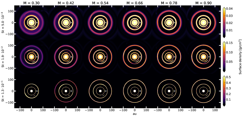
Figure 15: Dust surface density maps for a subset of three fluids with varying values of the planet 2 mass in $M_{\mathrm{jup}}$ at 500 orbits at $r_{0}$. The white crosses mark the position of planet 1.

In Fig. 15 a parameter study of the planet 2 mass influence is shown, involving the models p2m1 to p2m6. The nonaxisymmetric feature at the L5 point is sensitive to the mass of planet 2. In general, the passing of the planet acts as a perturber, inhibiting an effective dust trap in L5. The effect is visible in Fig. 15 for smaller grain sizes. Lower planet masses weaken the dust trapping in ring 2. We identify the balance between effective trapping in ring 2 and optimal dust trapping in the crescent-shaped feature to be on the order of $\approx 0.5M_{\mathrm{jup}}$, thus the choice of the fiducial model parameter.

Appendix B Resolution study

In the model fid_dres the resolution is doubled to $1120\times 1790$ cells in radial and azimuthal direction respectively compared to model fid. Fig. 16 indicates that an increased resolution leads to a more stable asymmetry in the Lagrange point L5. No decline in mass can be observed in the simulated time frame (1000 orbits at 48 au). The feature in the low resolution model fid however depletes rapidly after 600 orbits.
Since the dust trapped in this feature is sensitive to diffusive and disruptive effects, like e.g. viscosity, eccentricity and the passing of the outer planet, the accelerated dispersal may be attributed to numerical diffusion.
Quantifying the absolute value of the numerical diffusion is complex, however the order of magnitude can be estimated by a simple comparison of the high resolution run alpha3_dres with $\alpha=5\cdot 10^{-4}$ and the fiducial model. As shown in Fig. 10 the feature lifetime is approximately comparable to the one of the lower resolution run fid with a local $\alpha=2\cdot 10^{-4}$ . Therefore, the effect of the numerical diffusion in the low resolution model should be approximately equivalent to $\alpha\approx 5\cdot 10^{-4}$. Since FARGO3D is second-order accurate in space and the error of the dust module has been found to be proportional to a power law with an exponent of -2.2 as a function of the number of grid cells (Benítez-Llambay et al. 2019), the numerical diffusion is expected to be equivalent to $\alpha\approx 1\cdot 10^{-4}$ in the model fid_dres. The resolution is thus sufficient to describe the effect of prescribed local viscosity of $\alpha=2\cdot 10^{-4}$ .
Nevertheless, the absolute values of the amount of trapped dust mass in the stable phase is not significantly affected by the low resolution effect and lower resolution models are thus acceptable to quantify these values.

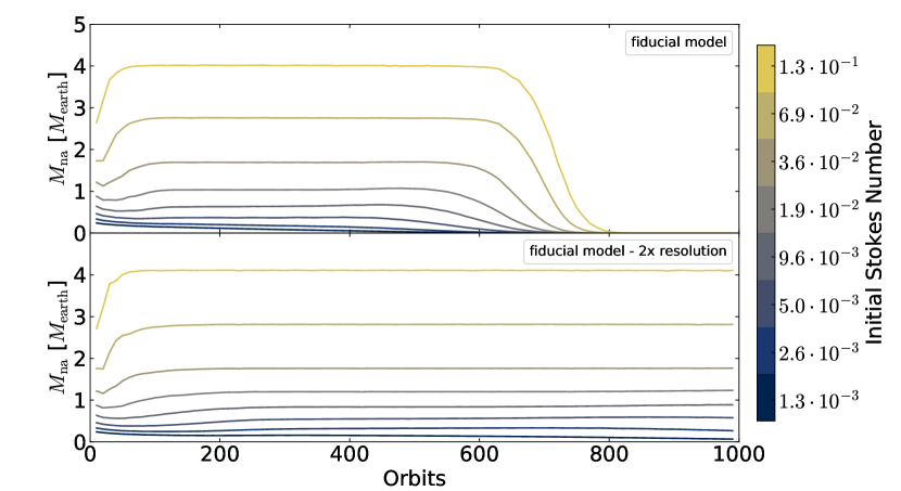
Figure 16: Development of the trapped dust mass in the L5 region of the simulations fid and fid_dres over time. In the lower panel the grid resolution is doubled in both the radial and azimuthal direction. The dispersal of the features are prolonged in the high resolution setup.

Appendix C Planet growth time scale

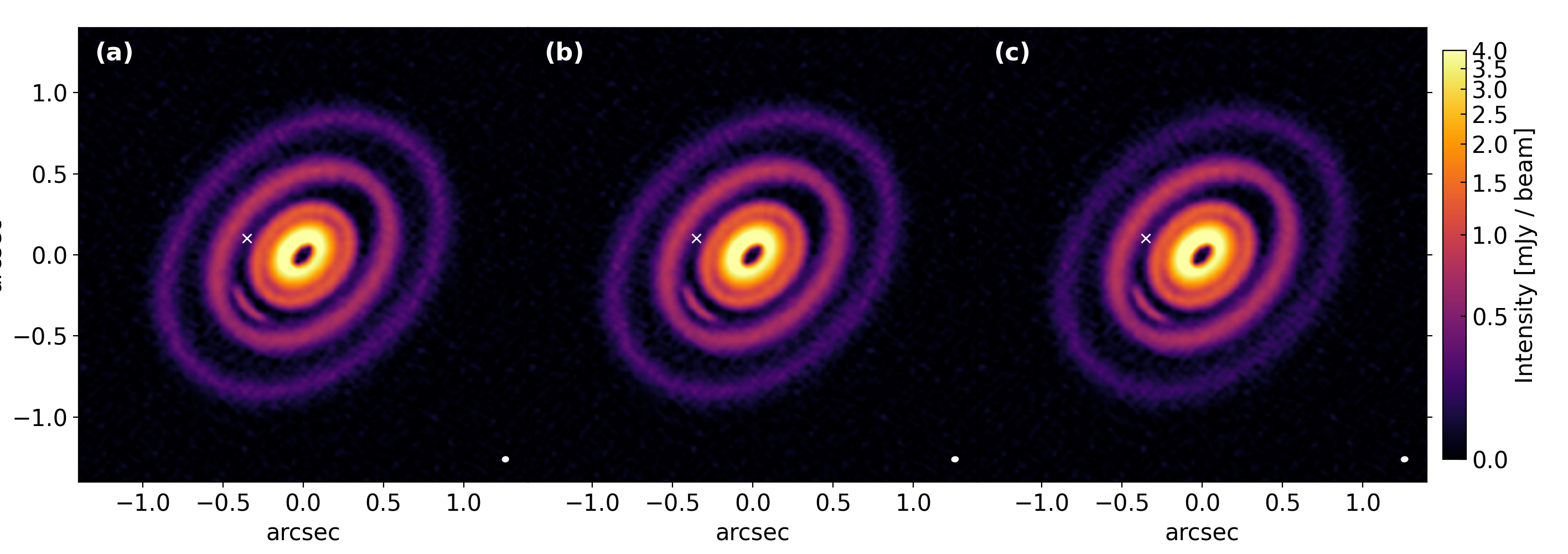
Figure 17: Comparison of the synthetic images of different planet growth time scales (a): $T_{\mathrm{G}}=10\,T_{0}$, (b): $T_{\mathrm{G}}=100\,T_{0}$, (c): $T_{\mathrm{G}}=500\,T_{0}$. The snapshots are taken after 2000 orbits at 48 au.

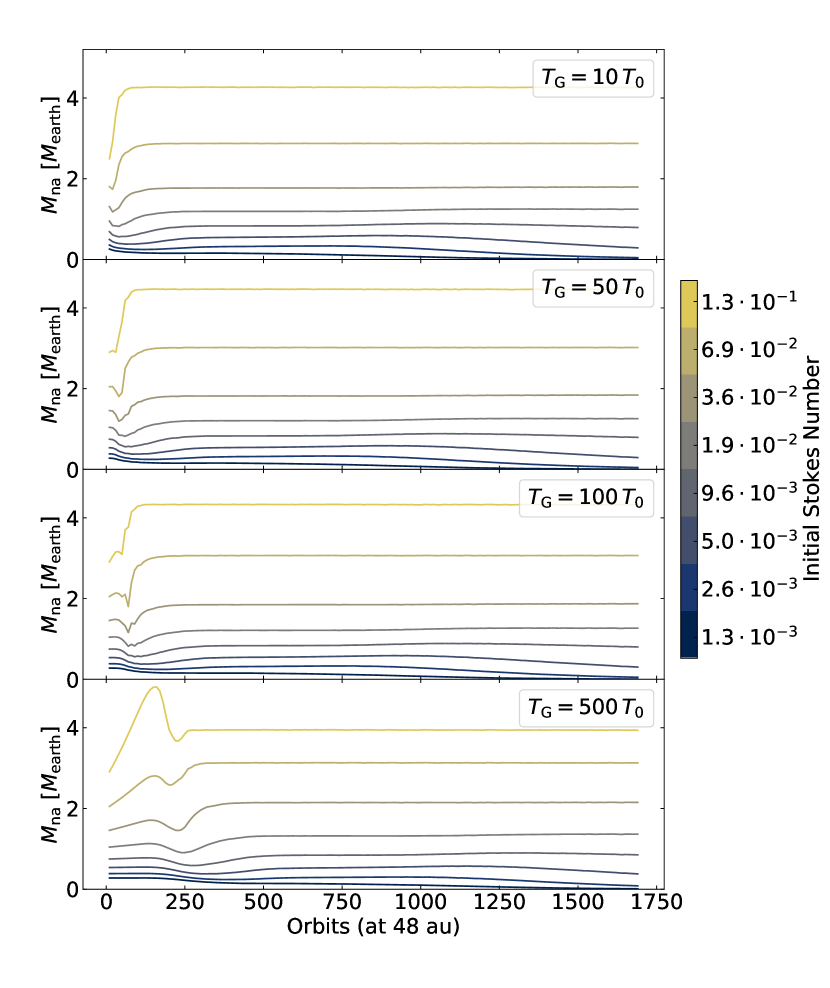
Figure 18: Evolution of the trapped dust mass $M_{\mathrm{na}}$ in the asymmetry around the L5 point for different planet growth time scales $T_{\mathrm{G}}$.

In Fig. 17 simulated ALMA observations are shown for planet mass growth time scales ranging from $T_{\mathrm{G}}=10\,T_{0}$ to $500\,T_{0}$. Ring 2 becomes less massive for longer planet growth time scales since dust drift depletes the outer regions before the planets reach a sufficiently high mass for efficient trapping.
The inner disk structure including the crescent-shaped asymmetry remains unaffected by the choice of parameters. Fig. 18 reveals the temporal evolution of the dust content in the asymmetry around the L5 point for all four growth time scales. For all runs grains smaller than $\approx 1\,\mathrm{mm}$ become depleted after more than 1000 orbits of evolution. After initial jumps in dust mass all simulations reach a stable stationary state considering millimeter grain sizes and above.

Appendix D Dust temperatures

In Fig. 19 dust temperatures from the radiative transfer calculation of the fiducial model and the prescribed gas temperatures are shown. While gas temperature gradient is smaller than the one for the dust, the temperatures and the slope of both match well at the location of planet 1, the primary region of interest where the crescent-shaped asymmetry forms. For the large grain sizes studied in this paper, a gray body approximation for the temperature is approximately valid. We thus see no significant increase in temperature comparing the grain sizes to each other.

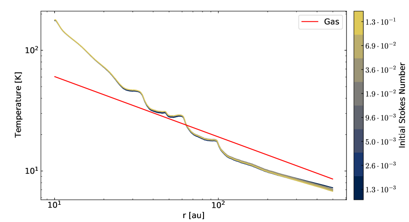
Figure 19: Comparison of prescribed gas temperature in the hydrodynamical simulation and the dust temperatures of the thermal Monte-Carlo calculation at the disk mid plane for all grain sizes.