Chiral hydrodynamics in strong external magnetic fields

Abstract

We construct the general hydrodynamic description of (3+1)-dimensional chiral charged (quantum) fluids subject to a strong external magnetic field with effective field theory methods. We determine the constitutive equations for the energy-momentum tensor and the axial charge current, in part from a generating functional. Furthermore, we derive the Kubo formulas which relate two-point functions of the energy-momentum tensor and charge current to 27 transport coefficients: 8 independent thermodynamic, 4 independent non-dissipative hydrodynamic, and 10 independent dissipative hydrodynamic transport coefficients. Five Onsager relations render 5 more transport coefficients dependent. We uncover four novel transport effects, which are encoded in what we call the shear-induced conductivity, the two expansion-induced longitudinal conductivities and the shear-induced Hall conductivity. Remarkably, the shear-induced Hall conductivity constitutes a novel non-dissipative transport effect. As a demonstration, we compute all transport coefficients explicitly in a strongly coupled quantum fluid via holography.

1 Introduction

Hydrodynamics is a universal effective field theory description of collective phenomena in (quantum) systems with many degrees of freedom. The hydrodynamic description of relativistic fluids has facilitated the physical interpretation of data from heavy ion collisions. It has also allowed to describe effects in condensed matter systems from charge conduction in metals to more recent descriptions of Weyl semimetals and graphene.

In this work, we consider the hydrodynamic description of a (3+1)-dimensional chiral charged thermal fluid subject to a strong external magnetic field. This is not to be confused with magnetohydrodynamics, in which the magnetic field satisfies Maxwell’s equations and hence is dynamical. Our external magnetic field is not dynamical in that sense. This magnetic field and the associated gauge potential $A_{\mu}$ can either be related to a vector $U(1)_{V}$ symmetry assumed to be preserved, or to an axial $U(1)_{A}$ symmetry which may be broken by a chiral anomaly. We point out the differences in the hydrodynamic description depending on which type of the two $U(1)$ symmetries is considered. Our focus, however, is the anomalous axial $U(1)_{A}$ case. We limit our considerations to zeroth and first order in the hydrodynamic derivative expansion. The magnetic field is referred to as strong if it is defined to be of zeroth order in derivatives. On a fundamental level, no axial magnetic fields exist in Nature. However, in low energy electronic descriptions for condensed matter systems such as Weyl-semimetals effectively axial magnetic fields and axial potentials can be created Cortijo_2015 ; Pikulin_2016 ; Grushin_2016 ; Cortijo:2016wnf . Thus we focus here on exploring the effects of an axial $U(1)_{A}$ symmetry. Based on previous results Hernandez:2017mch ; Son:2009tf ; Neiman:2010zi , we expect that adding a conserved vector current associated with a dynamical gauge field will not qualitatively change the physical effects, merely distribute them over different currents, introducing copies of analogous effects. Therefore, the hydrodynamic description derived here can be extended to be applied to the quark-gluon-plasma generated in heavy-ion-collisions.

Our main result are the Kubo formulas for the transport coefficients of a charged chiral thermal fluid subject to a strong magnetic field. These are derived in part from a generating functional and in part from constitutive relations which we construct in all generality in section 2. A nonzero strong magnetic field necessarily leads to anisotropic equilibrium states. In addition, an axial chemical potential breaks parity on the level of the state. The combination of these two broken symmetries explains the large number of transport coefficients. Specifically, we find 8 independent thermodynamic transport coefficients, and initially 19 hydrodynamic transport coefficients. Among the hydrodynamic transport coefficients we find 5 Onsager relations, which leaves 14 independent hydrodynamic transport coefficients. Of those hydrodynamic transport coefficients 3 are non-dissipative and 11 are dissipative. All independent transport coefficients are listed in tables 3, 4 and 5.

The first subset of the 8 independent thermodynamic transport coefficients are the well-known chiral conductivities: vortical $\xi=\xi_{TB}$, chiral magnetic $\xi_{B}$, and chiral thermal $\xi_{T}$. Referring to $\xi_{B}$ as “chiral magnetic effect” is a slight abuse of language. In most of this paper $\xi_{B}$ will measure the response of an axial current to an axial $U(1)_{A}$ magnetic field. The term “chiral magnetic effect” was coined for the response of such a current to a $U(1)_{V}$ vector magnetic field Kharzeev:2004ey , see also Jensen:2013vta . The remaining 5 thermodynamic transport coefficients are 4 newly non-vanishing susceptibilities: magneto-thermal $M_{1}$, perpendicular magneto-vortical $M_{2}$, magneto-acceleration $M_{3}$, magneto-electric $M_{4}$, and the previously discussed Kovtun:2016lfw ; Hernandez:2017mch magneto-vortical susceptibility $M_{5}$. The magneto-acceleration susceptibility $M_{3}$ vanishes in conformal field theories. Note that in addition there are three susceptibilities $\chi_{B}\,,\chi_{33},\,\chi_{13}$ which we do not include in our counting since they are thermodynamic partial derivatives of the pressure, $p$. In stark contrast to this, the $M_{n}$ ($n=1,\,2,\,3,\,4,\,5$) can not be defined as thermodynamic derivatives of the pressure, thus they are independent coefficients.

There are initially 19 hydrodynamic transport coefficients: the shear viscosities perpendicular and longitudinal to the magnetic field $\eta_{\perp},\,\eta_{||}$, the perpendicular and longitudinal Hall viscosities $\tilde{\eta}_{\perp},\,\tilde{\eta}_{||}$, the bulk viscosities $\zeta_{1}$, $\zeta_{2}$, $\eta_{1}$, $\eta_{2}$, the perpendicular and longitudinal charge conductivities $\sigma_{\perp}$, $\sigma_{||}$, the Hall conductivity $\tilde{\sigma}_{\perp}$ (which can alternately be expressed in terms of the charge resistivities $\rho_{\perp},\,\rho_{||},\,\tilde{\rho}_{\perp}$), and the novel $c_{3}$, $c_{4}$, $c_{5}$, $c_{8}$, $c_{10}$, $c_{14}$, $c_{15}$, $c_{17}$. Due to their effect on the fluid to be interpreted in section 2.5, we name $c_{8}$ the shear-induced conductivity, $c_{10}$ the shear-induced Hall conductivity, as well as $c_{4}$ and $c_{5}$ the expansion-induced longitudinal conductivities. Only 4 of the $c_{n}$’s (with $n=3,4,5,8,10,14,15,17$) are independent. Only 3 of the bulk viscosities are independent. This follows from 5 Onsager relations derived in this work.

In section 3, we prove the existence of these transport coefficients by direct computation of their nonzero values within the specific example of a strongly coupled $\mathcal{N}=4$ Super-Yang-Mills (SYM) theory at a large number of colors, $N_{c}\to\infty$, coupled to an external axial $U(1)_{A}$ gauge field. This computation is facilitated by holography Maldacena:1997re . In order to allow for a charged thermal state subject to a strong magnetic field, the charged magnetic black brane solutions are considered D'Hoker:2009bc . Within the classical gravity dual to SYM theory, we compute the frequency or momentum dependent fluctuations around the branes, which are holographically dual to field theory correlation functions of the energy momentum tensor and the axial current. Applying the Kubo formulas derived in section 2, we obtain nonzero values for most of the transport coefficients. An exception are the transport coefficients $c_{3}$, $M_{4},\,\tilde{\eta}_{\perp}$, $\zeta_{1}$ and $\zeta_{2}$ which vanish in the holographic model. The status of $M_{1}$ and $M_{3}$ is unclear within the holographic model as we only have Kubo relations for their derivatives. However, $M_{3}$ is expected to vanish due to conformal invariance.

The effect of chiral anomalies in hydrodynamics was first found through holographic calculations which yielded nonzero anomalous transport in Erdmenger:2008rm ; Banerjee:2008th ; Torabian:2009qk . More generally, the existence of anomalous transport as a consequence of chiral anomalies was elucidated in terms of a local version of the second law of thermodynamics in Son:2009tf . Subsequent studies of anomalous hydrodynamics include Neiman:2010zi ; Kharzeev:2009pj ; Kharzeev:2010gd ; Kharzeev:2013ffa ; Jensen:2012kj ; Jensen:2013kka ; Jensen:2013vta . The equilibrium partition function formulation of relativistic hydrodynamics was first introduced in Jensen:2012jh ; Banerjee:2012iz and subsequently used in a variety of settings Bhattacharyya:2012xi ; Bhattacharya:2012zx ; Bhattacharyya:2013ida ; Kovtun:2016lfw ; Hernandez:2017mch ; Kovtun:2018dvd ; Armas:2018zbe ; Kovtun:2019wjz . In particular, the equilibrium generating functional approach was used to formulate the hydrodynamic framework of (parity preserving) fluids subject to strong external as well as the framework of magnetohydrodynamics (when the electromagnetic field is dynamical) in Hernandez:2017mch . The relation between the frameworks of hydrodynamics with strong magnetic fields and magnetohydrodynamics, as well as the dual formulation of magnetohydrodynamics in terms of two-form fields introduced in Grozdanov:2016tdf was elucidated in Hernandez:2017mch . The anomaly inflow generating functionals have been used for anomalous hydrodynamics in equilibrium in Jensen:2013kka ; Jensen:2012kj and for out of equilibrium hydrodynamics in Haehl:2013hoa . Dispersion relations of hydrodynamic modes within the system under consideration in this work have been computed previously at weak magnetic fields of first order in the hydrodynamic derivative expansion Ammon:2017ded ; Kalaydzhyan:2016dyr ; Abbasi:2016rds . Anisotropic hydrodynamics has been discussed in the context of heavy ion collisions, see for example Martinez:2010sc ; Martinez:2010sd ; Ryblewski:2010bs ; Ryblewski:2011aq ; Ryblewski:2012rr ; Florkowski:2012lba ; Strickland:2014pga ; Huang:2011dc ; Ammon:2017ded .

Holographic duals of quantum field theories with a chiral anomaly and subject to weak electromagnetic fields (of first order in the hydrodynamic derivative expansion) have received much attention due to a host of applications that ranges from condensed matter physics to heavy ion collisions. Specific interest was focused on the analytically known Son:2009tf chiral conductivities: chiral magnetic effect Newman:2005hd ; Kharzeev:2004ey ; Kharzeev:2007jp ; Fukushima:2008xe ; Kharzeev:2009pj , the chiral vortical effect Vilenkin:1978is ; Vilenkin:1979ui ; Erdmenger:2008rm ; Banerjee:2008th , and later the chiral thermal conductivity, see e.g. Neiman:2010zi ; Ammon:2017ded . These (DC) conductivities have been shown to be exact in a multitude of holographic models Gursoy:2014boa ; Grozdanov:2016ala , and based on field theory arguments Fukushima:2008xe . (Non-)renormalization of these chiral conductivities was addressed holographically Gursoy:2014ela ; Jimenez-Alba:2014iia ; Gallegos:2018ozs and field theoretically Golkar:2012kb . The frequency dependent (AC) chiral conductivities have been discussed in Amado:2011zx ; Landsteiner:2013aba ; Li:2018srq , and from the field theory side in Kharzeev:2009pj . At nonzero value of the anomaly and without a strong magnetic field, analytic results for helicity-1 correlators in the hydrodynamic approximation have been obtained in Matsuo:2009xn . Without the anomaly, in strong magnetic field in an uncharged state Kubo formulas for seven transport coefficients have been derived and values were calculated numerically Grozdanov:2017kyl . The shear viscosities have been calculated in Critelli:2014kra ; PhysRevD.96.019903 under the assumption of the validity of the membrane paradigm. Dispersion relations of hydrodynamic and non-hydrodynamic modes within the system under consideration in this work have been computed from quasinormal modes previously at weak magnetic fields of first order in the hydrodynamic derivative expansion Ammon:2017ded . Quasinormal modes of magnetic black branes were calculated in Ammon:2016fru ; Janiszewski:2015ura ; Ammon:2017ded ; Baggioli:2020edn . In Grozdanov:2017kyl dynamical gauge fields in the dual field theory are considered within a two-form field formalism which is distinct from ours. See also Grozdanov:2016tdf ; Hernandez:2017mch for the relation between the two formalisms. Anisotropic effects not related to magnetic fields have also been included in holography in the hydrodynamic approximation Rebhan:2009vc ; Erdmenger:2010xm ; Erdmenger:2014jba ; Garbiso:2020puw .

2 Hydrodynamics

In this section, the constitutive equations, Kubo formulas, equilibrium generating functionals, as well as symmetry constraints, Onsager relations, and the entropy constraints are derived for a charged fluid subjected to a strong external magnetic field. Chemical potentials and magnetic fields associated with either an axial $U(1)_{A}$-symmetry or a vector $U(1)_{V}$-symmetry are considered. Quantities can be classified according to their charge under a parity transformation of the three spatial coordinates in a field theory fluid state. It is helpful to notice that there are three potential sources for parity breaking in the fluids we consider: the chiral anomaly in the microscopic field theory, the external magnetic field associated with a vector $U(1)_{V}$-symmetry, or the axial chemical potential if a global axial $U(1)_{A}$-symmetry is considered. In order to derive constitutive relations and Kubo formulas, we will use generating functionals among other methods. Note that the generating functionals (2), (16) and (21) in presence of a global axial $U(1)_{A}$-symmetry transforms even under charge-inversion, parity, and time-reversal, i.e. it has $(C,P,T)$-eigenvalues (+/+/+).

2.1 Thermodynamics

2.1.1 Generating functional and equilibrium constitutive relations

Following the procedure proposed in Banerjee:2012iz ; Jensen:2012jh , we begin by considering the equilibrium constraints on the hydrodynamic framework arising from the existence of a static generating functional. These constraints arise from considering a system with a time-like Killing vector field $V$ (i.e. ${\cal L}_{V}=0$) coupled to an external metric $g$ and gauge field $A$. For systems that

• have finite correlation lengths,

• are in equilibrium (${\cal L}_{V}=0)$,

• have sources $g,A$ that vary on scales much longer than the correlation lengths,

the generating functional $W_{s}[g,A]=-i\,{\rm ln}Z[g,A]$ is a local functional of the Killing vector field and the sources. The equilibrium generating functional can be systematically expanded in a derivative expansion. The temperature $T$, the chemical potential $\mu$ and the fluid velocity $u^{\mu}$, which are traditionally considered the only zero derivative terms and are defined in terms of the Killing vector field and the sources

$$T=\frac{T_{0}}{\sqrt{-V^{2}}}\,,\quad u^{\mu}=\frac{V^{\mu}}{\sqrt{-V^{2}}}\,,\quad\mu=\frac{V^{\mu}A_{\mu}+\Lambda_{V}}{\sqrt{-V^{2}}}\,,$$ (1)

where $T_{0}$ is a constant setting the normalization of the temperature, and $\Lambda_{V}$ is a gauge parameter which ensures that $\mu$ is gauge invariant Jensen:2013kka . In addition, for a system subject to a strong magnetic field $B^{\mu}=\frac{1}{2}\epsilon^{\mu\nu\rho\sigma}u_{\nu}F_{\rho\sigma}\sim{\cal O}(1)$, the scalar $B^{2}=B^{\mu}B^{\nu}g_{\mu\nu}$ is order zero in derivatives as well. In this paper, we assume the counting $T,\mu,u^{\mu},B^{\mu}\sim{\cal O}(1)$ and all other terms with a derivative as ${\cal O}(\partial)$. For example, $E_{\mu}=F_{\mu\nu}u^{\nu}\sim{\cal O}(\partial)$ and $R^{\mu}_{\ \nu\rho\sigma}\sim\partial\partial g\sim{\cal O}(\partial^{2})$. In addition, the derivatives of the fluid velocity such as the vorticity $\Omega^{\mu}=\epsilon^{\mu\nu\rho\sigma}u_{\nu}\partial_{\rho}u_{\sigma}$ and the fluid acceleration $a^{\mu}=u^{\nu}\nabla_{\nu}u^{\mu}$ are $\mathcal{O}(\partial)$. In table 6, the behavior of hydrodynamic fields, sources and other quantities under charge conjugation $C$, parity $P$, and time reversal $T$ are collected. Note that in this subsection on equilibrium states, the only parity violation stems from the axial gauge field and the associated axial chemical potential.

With this derivative counting, the equilibrium generating functional for a hydrodynamic system coupled to external gauge field and metric subject to strong magnetic fields can be expanded as Hernandez:2017mch

$$W_{s}=\int d^{4}x\sqrt{-g}\left(p(T,\mu,B^{2})+\sum_{n=1}^{5}M_{n}(T,\mu,B^{2})s_{n}+O(\partial^{2})\right)\,,$$ (2)

where $p$ is the homogeneous equilibrium pressure and $s_{n}$ are the first order equilibrium scalars, that is, $s_{n}\sim{\cal O}(\partial)$. Their definitions are listed in table 1, together with their transformation properties under charge conjugation, parity, time reversal and Weyl transformations. The magnetovortical susceptibility $M_{5}=M_{\Omega}$ is the only nonzero first order thermodynamic function for a parity-preserving theory coupled to vector gauge fields. On the other hand, for a system coupled to an axial gauge field, the axial chemical potential $\mu$ breaks parity and the other $M_{n}$ can in principle be nonzero. These will appear along with the pressure in the thermodynamic/hydrostatic constitutive relations. We stress that, in absence of the chiral anomaly, the microscopic theory does not break the parity symmetry, but rather the state in question breaks parity, provided there is a nonzero axial chemical potential. Table 1 highlights the symmetry properties of the equilibrium scalars when defined in terms of axial gauge fields. For this paper, we will focus in the case where our system is coupled to axial gauge fields. This requires us to include the terms that are usually considered to be parity-violating when considering vector gauge fields. That is, the $M_{1}$, $M_{2}$, $M_{3}$ and $M_{4}$ can be nonzero for a parity preserving system coupled to an external axial gauge field. In this section, we elaborate on the modifications of the hydrodynamic framework when these terms are included.

We will write the energy-momentum tensor using the decomposition with respect to the timelike velocity vector $u^{\mu}$,

$$T^{\mu\nu}={\cal E}u^{\mu}u^{\nu}+{\cal P}\Delta^{\mu\nu}+{\cal Q}^{\mu}u^{\nu}+{\cal Q}^{\nu}u^{\mu}+{\cal T}^{\mu\nu}\,,$$ (3)

where $\Delta^{\mu\nu}\equiv g^{\mu\nu}+u^{\mu}u^{\nu}$ is the transverse projector, the energy current ${\cal Q}^{\mu}$ is transverse to $u_{\mu}$, and ${\cal T}^{\mu\nu}$ is transverse to $u_{\mu}$, symmetric, and traceless. Explicitly, the coefficients are ${\cal E}\equiv u_{\mu}u_{\nu}T^{\mu\nu}$, ${\cal P}\equiv{\textstyle{\frac{1}{3}}}\Delta_{\mu\nu}T^{\mu\nu}$, ${\cal Q}_{\mu}\equiv-\Delta_{\mu\alpha}u_{\beta}T^{\alpha\beta}$ and ${\cal T}_{\mu\nu}\equiv{\textstyle{\frac{1}{2}}}(\Delta_{\mu\alpha}\Delta_{\nu\beta}+\Delta_{\nu\alpha}\Delta_{\mu\beta}-{\textstyle{\frac{2}{3}}}\Delta_{\mu\nu}\Delta_{\alpha\beta})T^{\alpha\beta}$. Similarly, we will write the current as

$$J^{\mu}={\cal N}u^{\mu}+{\cal J}^{\mu}\,,$$ (4)

where the charge density is ${\cal N}\equiv-u_{\mu}J^{\mu}$, and the spatial current is ${\cal J}_{\mu}\equiv\Delta_{\mu\lambda}J^{\lambda}$. We also decompose the field strength tensor with respect to $u^{\mu}$,

$n$	1	2	3	4	5
$s_{n}$	$B^{\mu}\partial_{\mu}(\frac{B^{2}}{T^{4}})$	$\epsilon^{\mu\nu\rho\sigma}u_{\mu}B_{\nu}\nabla_{\!\rho}B_{\sigma}$	$B{\cdot}a$	$B{\cdot}E$	$B{\cdot}\Omega$
$(C,P,T)_{\textrm{axial}}$	$+/+/-$	$+/-/+$	$+/+/-$	$+/-/-$	$+/-/+$
$(C,P,T)_{\textrm{vector}}$	$-/-/-$	$+/-/+$	$-/-/-$	$+/-/-$	$-/+/+$
W	3	5	n/a	4	3

Table 1: Independent nonzero $O(\partial)$ invariants in equilibrium in 3+1 dimensions for an axial gauge field. We have used the fluid acceleration $a^{\mu}=u^{\lambda}\nabla_{\lambda}u^{\mu}$ and the vorticity $\Omega^{\mu}=\epsilon^{\mu\nu\rho\sigma}u_{\nu}\partial_{\rho}u_{\sigma}$. An axial chemical potential $\mu$ is $C$-even and $P$-odd. In case of an axial chemical potential we expect $M_{1}$ and $M_{3}$ to be even functions of $\mu$ while $M_{2}$, $M_{4}$ and $M_{5}$ should be odd functions of $\mu$. Here the last row labelled “W” indicates the charge under Weyl-transformations and “n/a” indicates that the tensor structure $s_{3}$ does not have a definite behavior under Weyl-transformations.

$$F_{\mu\nu}=u_{\mu}E_{\nu}-u_{\nu}E_{\mu}-\epsilon_{\mu\nu\rho\sigma}u^{\rho}B^{\sigma}\,,$$ (5)

where $E_{\mu}=F_{\mu\nu}u^{\nu}$ is the electric field and $B^{\mu}={\textstyle{\frac{1}{2}}}\epsilon^{\mu\nu\rho\sigma}u_{\nu}F_{\rho\sigma}$ is the magnetic field. We use the convention $\epsilon^{\mu\nu\rho\sigma}=\varepsilon^{\mu\nu\rho\sigma}/\sqrt{-g}$, where $\varepsilon^{0123}=1$. We also use the vorticity $\Omega^{\mu}=\epsilon^{\mu\nu\rho\sigma}u_{\nu}\partial_{\rho}u_{\sigma}$.

The equilibrium constitutive relations are found by varying the generating functional with respect to the metric and the gauge field

$$\delta W_{s}[A,g]=\int d^{4}x\sqrt{-g}\left({\textstyle{\frac{1}{2}}}T^{\mu\nu}_{\rm eq.}\delta g_{\mu\nu}+J^{\mu}_{\rm eq.}\delta A_{\mu}\right)\,.$$ (6)

This was done in Hernandez:2017mch for a parity-preserving theory coupled to a vector gauge field. The new terms allowed when considering an axial gauge field come from the variation of $M_{i}(T,\mu,B^{2})S_{i}$ for $i\neq 5$ and are given by

$${\cal E}_{{\rm eq.\,new}}=\sum_{n=1}^{4}\epsilon_{n}s_{n}\,,\quad{\cal P}_{\rm eq.\,new}=\sum_{n=1}^{4}\pi_{n}s_{n}\,,\quad{\cal N}_{\rm eq.\,new}=\sum_{n=1}^{4}s_{n}\,\quad{\cal T}^{\mu\nu}_{{\rm eq.\,new}}=\sum_{n=1}^{10}\theta_{n}\tau^{\mu\nu}_{n}\,,$$ (7)

where

$$\epsilon_{3}=-\frac{4B^{2}}{T^{4}}\epsilon_{1}=3\pi_{3}=-4B^{2}\theta_{3}=\frac{4B^{2}}{T^{4}}\left(M_{1}-TM_{1,T}-\mu M_{1,\mu}-4B^{2}M_{1,B^{2}}-T^{4}M_{3,B^{2}}\right)\,,$$ (8)

$$\epsilon_{2}=\theta_{6}=-M_{2}+TM_{2,T}+\mu M_{2,\mu}\,,\quad\epsilon_{4}=TM_{4,T}+\mu M_{4,\mu}+\frac{4B^{2}}{T^{4}}M_{1,\mu}+M_{3,\mu}\,,$$

$$\pi_{2}=-{\textstyle{\frac{2}{3}}}M_{2}-{\textstyle{\frac{4}{3}}}B^{2}M_{2,B^{2}}\,,n\quad\pi_{4}=-{\textstyle{\frac{4}{3}}}B^{3}\theta_{4}=\frac{4B^{2}}{3T^{4}}\phi_{1}=\frac{4B^{2}}{3T^{4}}\left(M_{1,\mu}-T^{4}M_{4,B^{2}}\right)\,,$$

$$\phi_{2}=M_{2,\mu}\,,\quad\phi_{3}=\epsilon_{4}-3\pi_{4}\,,\quad\theta_{2}=M_{2,B^{2}}\,,\quad\theta_{5}=2M_{2}\,,\quad\theta_{7}=M_{2,B^{2}}\,,\quad\theta_{8}=-M_{2,\mu}\,,$$

$$\pi_{1}=\phi_{4}=\theta_{1}=0\,.$$

The comma subscript denotes the derivative with respect to the argument that follows, and we are using $(T,\mu,B^{2})$ as our three independent variables. Hence, for example, $M_{1,T}=\left(\frac{\partial M_{1}}{\partial T}\right)_{\mu,B^{2}}$. The equilibrium vectors and tensors are defined in table 2. The equilibrium spatial current $\mathcal{J}^{\mu}$ and energy current $\mathcal{Q}^{\mu}$ do not receive contributions to $O(\partial)$ from the novel thermodynamic transport coefficients $M_{1}$, $M_{2}$, $M_{3}$ and $M_{4}$.

$n$	1	2	3	4
$v_{n}^{\mu}$	$\epsilon^{\mu\nu\rho\sigma}u_{\nu}\partial_{\sigma}B_{\rho}$	$\epsilon^{\mu\nu\rho\sigma}u_{\nu}B_{\rho}\partial_{\sigma}T/T$	$\epsilon^{\mu\nu\rho\sigma}u_{\nu}B_{\rho}\partial_{\sigma}B^{2}$	$\epsilon^{\mu\nu\rho\sigma}u_{\nu}E_{\rho}B_{\sigma}$

$n$	$1-4$	5	6	7	8
$t_{n}^{\mu\nu}$	$s_{n}B^{\langle\mu}B^{\nu\rangle}$	$v_{1}^{\langle\mu}B^{\nu\rangle}$	$v_{2}^{\langle\mu}B^{\nu\rangle}$	$v_{3}^{\langle\mu}B^{\nu\rangle}$	$v_{4}^{\langle\mu}B^{\nu\rangle}$

Table 2: Top: nonzero transverse $O(\partial)$ vectors that appear in the parity-violating equilibrium energy flux ${\cal Q}^{\mu}$ and in the equilibrium spatial current ${\cal J}^{\mu}$. The vector $v_{4}^{\mu}$ is the Poynting vector. Bottom: nonzero symmetric transverse traceless $O(\partial)$ tensors that appear in the equilibrium stress ${\cal T}^{\mu\nu}$. For any two transverse vectors $X^{\mu}$ and $Y^{\mu}$, the angular brackets stand for $X^{\langle\mu}Y^{\nu\rangle}\equiv X^{\mu}Y^{\nu}+X^{\nu}Y^{\mu}-{\textstyle{\frac{2}{3}}}\Delta^{\mu\nu}X{\cdot}Y$.

For a diffeomorphism and gauge invariant theory, invariance of the generating functional gives the following hydrodynamic equations

$$\nabla_{\nu}T^{\mu\nu}=F^{\mu\nu}J_{\nu}\,,$$ (9a)

$$\nabla_{\mu}J^{\mu}=0\,.$$ (9b)

The definition of the equilibrium energy-momentum tensor and conserved currents ensure that the equations of motion are satisfied in equilibrium.

For completeness, let us summarize the equilibrium constitutive relations for the energy-momentum tensor and the current. The equilibrium energy-momentum tensor is given by

$${\cal E}_{\rm eq.} =-p+T\,p_{,T}+\mu\,p_{,\mu}+\left(T{{M_{5}}}_{,T}+\mu{{M_{5}}}_{,\mu}-2{M_{5}}\right)B{\cdot}\Omega$$

$$\ \ \ \,+\left(TM_{1,T}+\mu M_{1,\mu}+4B^{2}M_{1,B^{2}}+T^{4}M_{3,B^{2}}-M_{1}\right)s_{1}$$

$$\ \ \ \,+\left(TM_{2,T}+\mu M_{2,\mu}-M_{2}\right)s_{2}$$

$$\ \ \ \,+\frac{4B^{2}}{T^{4}}\left(M_{1}-TM_{1,T}-\mu M_{1,\mu}-4B^{2}M_{1,B^{2}}-T^{4}M_{3,B^{2}}\right)s_{3}$$

$$\ \ \ \,+\left(TM_{4,T}+\mu M_{4,\mu}+\frac{4B^{2}}{T^{4}}M_{1,\mu}+M_{3,\mu}\right)s_{4}\,,$$ (10a)

$${\cal P}_{\rm eq.} =p-{\textstyle{\frac{4}{3}}}\,p_{,B^{2}}B^{2}-{\textstyle{\frac{1}{3}}}({M_{5}}+4{{M_{5}}}_{,B^{2}}B^{2})B{\cdot}\Omega-{\textstyle{\frac{2}{3}}}\left(M_{2}+2B^{2}M_{2,B^{2}}\right)s_{2}$$

$$\ \ \ \,+\frac{4B^{2}}{3T^{4}}\left(M_{1}-TM_{1,T}-\mu M_{1,\mu}-4B^{2}M_{1,B^{2}}-T^{4}M_{3,B^{2}}\right)s_{3}$$

$$\ \ \ \,+\frac{4B^{2}}{3T^{4}}\left(M_{1,\mu}-T^{4}M_{4,B^{2}}\right)s_{4}\,,$$ (10b)

$${\cal Q}^{\mu}_{\rm eq.} =-{M_{5}}\epsilon^{\mu\nu\rho\sigma}u_{\nu}\partial_{\sigma}B_{\rho}+(2{M_{5}}-T{{M_{5}}}_{,T}-\mu{{M_{5}}}_{,\mu})\epsilon^{\mu\nu\rho\sigma}u_{\nu}B_{\rho}\partial_{\sigma}T/T$$

$$\ \ \ \,-{{M_{5}}}_{,B^{2}}\epsilon^{\mu\nu\rho\sigma}u_{\nu}B_{\rho}\partial_{\sigma}B^{2}+({{M_{5}}}_{,\mu}-2p_{,B^{2}})\epsilon^{\mu\nu\rho\sigma}u_{\nu}E_{\rho}B_{\sigma}$$ (10c)

$${\cal T}^{\mu\nu}_{\rm eq.} =2p_{,B^{2}}\left(B^{\mu}B^{\nu}-{\textstyle{\frac{1}{3}}}\Delta^{\mu\nu}B^{2}\right)+B^{\langle\mu}B^{\nu\rangle}\left({{M_{5}}}_{,B^{2}}B{\cdot}\Omega+M_{2,B^{2}}s_{2}+(M_{4,B^{2}}-{\textstyle{\frac{1}{T^{4}}}}M_{1,\mu})s_{4}\right)$$

$$\ \ \ \,+B^{\langle\mu}B^{\nu\rangle}\frac{1}{T^{4}}\left(TM_{1,T}+\mu M_{1,\mu}+4B^{2}M_{1,B^{2}}-M_{1}+T^{4}M_{3,B^{2}}\right)s_{3}+{M_{5}}B^{\langle\mu}\Omega^{\nu\rangle}$$

$$\ \ \ \,+2M_{2}B^{\langle\mu}\epsilon^{\nu\rangle\rho\sigma\alpha}u_{\rho}\partial_{\sigma}B_{\alpha}+\left(TM_{2,T}+\mu M_{2,\mu}-M_{2}\right)B^{\langle\mu}\epsilon^{\nu\rangle\alpha\rho\sigma}u_{\alpha}B_{\rho}\partial_{\sigma}T/T$$

$$\ \ \ \,+M_{2,B^{2}}B^{\langle\mu}\epsilon^{\nu\rangle\alpha\rho\sigma}u_{\alpha}B_{\rho}\partial_{\sigma}B^{2}-M_{2,\mu}B^{\langle\mu}\epsilon^{\nu\rangle\rho\sigma\alpha}u_{\rho}E_{\sigma}B_{\alpha}\,,$$ (10d)

where we used the vorticity $\Omega^{\mu}=\epsilon^{\mu\nu\rho\sigma}u_{\nu}\partial_{\rho}u_{\sigma}$. The current is given by

$${\cal N}_{\rm eq.} =p_{,\mu}-\nabla{\cdot}\mathfrak{p}+\mathfrak{p}{\cdot}a-\mathfrak{m}{\cdot}\Omega+\left(M_{1,\mu}-T^{4}M_{4,B^{2}}\right)s_{1}+M_{2,\mu}s_{2}$$

$$\ \ \ \,+\left(M_{3,\mu}+TM_{4,T}+\mu M_{4,\mu}+4B^{2}M_{4,B^{2}}\right)s_{3}+{{M_{5}}}_{,\mu}s_{5}\,,$$ (11a)

$${\cal J}^{\mu}_{\rm eq.} =\epsilon^{\mu\nu\rho\sigma}u_{\nu}\nabla_{\!\rho}\mathfrak{m}_{\sigma}+\epsilon^{\mu\nu\rho\sigma}u_{\nu}a_{\rho}\mathfrak{m}_{\sigma}\,,$$ (11b)

where $a^{\mu}=u^{\lambda}\nabla_{\lambda}u^{\mu}$ defines the acceleration and the (electric) polarization vector is $\mathfrak{p}_{\mu}=\frac{1}{\sqrt{-g}}\frac{\delta W_{s}}{\delta E^{\mu}}=M_{4}B_{\mu}$. The current is written in terms of the magnetic polarization vector $\mathfrak{m}_{\mu}=\frac{1}{\sqrt{-g}}\frac{\delta W_{s}}{\delta B^{\mu}}$

$$\mathfrak{m}^{\mu} =\left(2\,p_{,B^{2}}+2\sum_{n=2}^{5}M_{n,B^{2}}s_{n}+\frac{2}{T^{4}}\left(M_{1}-TM_{1,T}-\mu M_{1,\mu}-4B^{2}M_{1,B^{2}}\right)B{\cdot}\partial T/T\right)B^{\mu}$$ (12)

$$\ \ \ \,+{M_{5}}\Omega^{\mu}+M_{3}a^{\mu}+M_{4}E^{\mu}+M_{1}\Delta^{\mu\nu}\partial_{\nu}\frac{B^{2}}{T^{4}}-M_{2,\mu}\epsilon^{\mu\nu\rho\sigma}u_{\nu}E_{\rho}B_{\sigma}+M_{2,B^{2}}\epsilon^{\mu\nu\rho\sigma}u_{\nu}B_{\rho}\partial_{\sigma}B^{2}$$

$$\ \ \ \,+\left(TM_{2,T}+\mu M_{2,\mu}-M_{2}\right)\epsilon^{\mu\nu\rho\sigma}u_{\nu}B_{\rho}\partial_{\sigma}T/T+2M_{2}\epsilon^{\mu\nu\rho\sigma}u_{\nu}\partial_{\rho}B_{\sigma}\,.$$

Note that we are keeping O($\partial^{2}$) thermodynamic terms in the current (coming from the variation of $\sum_{n=1}^{5}M_{n}s_{n}$ in the generating functional) that are needed to ensure that the conservation laws (9) are satisfied to $O(\partial^{2})$ for time-independent background fields. Including the $O(\partial^{2})$ thermodynamic terms in the energy-momentum tensor will ensure these are satisfied identically, but we omit them here for simplicity.

2.1.2 Incorporating the chiral anomaly

For a theory with a chiral anomaly subject to external axial gauge fields, the generating functional is no longer gauge invariant,

$$\delta_{\alpha}W_{cons}=\frac{C}{24}\int d^{4}x\sqrt{-g}\,\alpha\,\epsilon^{\mu\nu\rho\sigma}F_{\mu\nu}F_{\rho\sigma}\equiv{\cal A}\,,$$ (13)

leading to the following

$$\nabla_{\mu}T^{\mu\nu}_{A}=F^{\mu\nu}J^{cons}_{\nu}-A^{\nu}\nabla_{\mu}J^{\mu}_{cons}\,,$$ (14a)

$$\nabla_{\mu}J_{cons}^{\mu}=-\frac{C}{24}\epsilon^{\mu\nu\rho\sigma}F_{\mu\nu}F_{\rho\sigma}=\frac{C}{3}E{\cdot}B\,,$$ (14b)

where $J_{cons}^{\mu}=\frac{1}{\sqrt{-g}}\frac{\delta W_{cons}}{\delta A_{\mu}}$ is the gauge dependent consistent current. The fact that it is gauge dependent follows from the commuting of $\frac{\delta}{\delta A_{\mu}}$ with the BRST operator $s=\int d^{4}x\partial_{\mu}c\frac{\delta}{\delta A_{\mu}}$ generating gauge transformations, from which we get $\delta_{\alpha}J^{\mu}_{cons}=\frac{1}{\sqrt{-g}}\frac{\delta}{\delta A_{\mu}}{\cal A}={\textstyle{\frac{1}{6}}}C\epsilon^{\mu\nu\rho\sigma}\partial_{\nu}\alpha F_{\rho\sigma}$. Noting that ${\cal A}$ is independent of the metric, a similar argument shows that the consistent energy-momentum tensor $T^{\mu\nu}_{A}=\frac{2}{\sqrt{-g}}\frac{\delta W_{cons}}{\delta g_{\mu\nu}}$ is gauge invariant. It is possible to add a Chern-Simons current $J^{\mu}_{BZ}=-{\textstyle{\frac{1}{6}}}C\epsilon^{\mu\nu\rho\sigma}A_{\nu}F_{\rho\sigma}$, also known as a Bardeen-Zumino polynomial, to the consistent current to get a gauge invariant current $J^{\mu}_{cov}$, usually named covariant current. The equations of motion (14) then take the manifestly gauge covariant from

$$\nabla_{\nu}T^{\mu\nu}_{A}=F^{\mu\nu}J^{cov}_{\nu}\,,$$ (15a)

$$\nabla_{\mu}J^{\mu}_{cov}=-\frac{C}{8}\epsilon^{\mu\nu\rho\sigma}F_{\mu\nu}F_{\rho\sigma}=CE{\cdot}B\,.$$ (15b)

Note that the covariant energy-momentum tensor is the same as the consistent energy-momentum tensor. See Landsteiner:2016led for a recent review on anomalous currents.

To understand how this gauge anomaly affects the hydrodynamic description, we construct the equilibrium generating functionals for the consistent and for the covariant currents using the anomaly inflow mechanism Callan:1984sa . The anomaly inflow generating functionals have been used for anomalous hydrodynamics in equilibrium in Jensen:2013kka ; Jensen:2012kj and for out of equilibrium hydrodynamics in Haehl:2013hoa .

The gauge dependent generating functional for the consistent current of a 3+1 dimensional theory is given by

$$W_{cons}=W_{s}+\int d^{4}x\sqrt{-g}\left(c_{1}T^{2}\Omega{\cdot}A+c_{2}T\left(B{\cdot}A+\mu\Omega{\cdot}A\right)+\frac{C}{3}\mu\left(B{\cdot}A+{\textstyle{\frac{1}{2}}}\mu\Omega{\cdot}A\right)\right)\,,$$ (16)

where $W_{s}$ is the generating functional for a theory without anomalies (2). We refer to $W_{cons}$ as the consistent generating functional. The vectors $T^{2}\Omega^{\mu}$ and $TB^{\mu}+T\mu\Omega^{\mu}$ have vanishing divergence and do not contribute to the gauge anomaly, unless the 3+1-dimensional theory has a boundary. The gauge dependence of the consistent generating functional (13) comes from the non-conservation of the vector $\nabla_{\mu}\left(\mu B^{\mu}+{\textstyle{\frac{1}{2}}}\mu^{2}\Omega^{\mu}\right)=B{\cdot}E$. Note that the term multiplying $c_{2}$ breaks CPT symmetry and is therefore not allowed for Lorentz invariant theories Jensen:2013vta . The coefficient $c_{1}$ is related to the mixed gauge-gravitational anomaly $c_{m}$ by Chen:2012ca ; Jensen:2012kj ; Landsteiner:2011cp ; Stone:2018zel ; Landsteiner:2011iq

$$c_{1}=-8\pi^{2}c_{m}\,.$$ (17)

The variation of the consistent generating functional yields the energy-momentum tensor and the consistent current. We now focus on the new terms coming from $W_{cons}-W_{s}$ and write $\Delta J_{cons}^{\mu}=J^{\mu}_{cons}-J^{\mu}$ where $J^{\mu}$ is the current found in eq. (6) by varying $W_{s}$. Similarly, we write $\Delta T^{\mu\nu}=T^{\mu\nu}_{A}-T^{\mu\nu}$ where $T^{\mu\nu}$ comes from varying $W_{s}$. Taking the source variations we find

$$\Delta T^{\mu\nu} =\xi_{T}u^{(\mu}\Omega^{\nu)}+\xi_{TB}\,u^{(\mu}B^{\nu)}\,,$$ (18a)

$$\Delta J^{\mu}_{cons} ={\textstyle{\frac{1}{3}}}CB{\cdot}Au^{\mu}+\xi\,\Omega^{\mu}+\left(\xi_{B}-{\textstyle{\frac{1}{3}}}C\mu\right)B^{\mu}+{\textstyle{\frac{1}{3}}}C\epsilon^{\mu\nu\rho\sigma}A_{\nu}u_{\rho}E_{\sigma}\,,$$ (18b)

where

$$\xi ={\textstyle{\frac{1}{2}}}C\mu^{2}+c_{1}T^{2}+2c_{2}T\mu\,,\quad \xi_{B}=C\mu+2c_{2}T\,,$$

$$\xi_{T} ={\textstyle{\frac{1}{3}}}C\mu^{3}+2c_{1}T^{2}\mu+2c_{2}T\mu^{2}\,,\quad \xi_{TB}={\textstyle{\frac{1}{2}}}C\mu^{2}+c_{1}T^{2}+2c_{2}T\mu\,.$$ (19)

The consistent current $J^{\mu}_{cons}$ and energy-momentum tensor $T^{\mu\nu}_{A}$ satisfy the consistent equations of motion (14) derived from the diffeomorphism invariance and gauge-non-invariance of the consistent generating functional $W_{cons}$. From the consistent current, we can construct the covariant current $J^{\mu}_{cov}$ by adding to it the Bardeen-Zumino/Chern-Simons current $J^{\mu}_{BZ}=-{\textstyle{\frac{1}{6}}}C\epsilon^{\mu\nu\rho\sigma}A_{\nu}F_{\rho\sigma}$,

$$J^{\mu}_{cov}=J^{\mu}_{cons}+J^{\mu}_{BZ}\,.$$ (20)

Alternatively, we can construct a covariant generating functional $W_{cov}$ by adding a Chern-Simons functional to the consistent generating functional

$$W_{cov}=W_{cons}+W_{CS}\,,$$ (21)

where

$$W_{CS}=-\frac{C}{6}\int A\wedge F\wedge F=-\frac{C}{24}\int d^{5}x\sqrt{-G}\epsilon^{mnopq}A_{m}F_{no}F_{pq}\,.$$ (22)

We take our Chern-Simons theory to live in a 4+1 dimensional space-time ${\cal M}$ with a boundary $\partial{\cal M}$ which corresponds to the space-time where $W_{cons}$ is defined. The five dimensional field strength $F_{mn}=\partial_{m}A_{n}-\partial_{n}A_{m}$ is defined in terms of the five dimensional gauge field $A_{m}$. We take the gauge field $A_{\mu}$ appearing in $W_{cons}$ as the induced gauge field on $\partial{\cal M}$ from $A_{m}$. The Chern-Simons functional is independent of the five dimensional metric $G_{mn}$, and we use the convention $\epsilon^{mnopq}=\varepsilon^{mnopq}/\sqrt{-G}$, where $\varepsilon^{0123z}=1$ and z is the coordinate normal to $\partial{\cal M}$. We also take $G_{mn}$ so that the induced metric in $\partial{\cal M}$ is $g_{\mu\nu}$, the metric used in the consistent generating functional. The Chern-Simons theory is gauge invariant up to a boundary term

$$\delta_{\alpha}W_{CS}=-\frac{C}{24}\int_{\partial{\cal M}}d^{4}x\sqrt{-g}\alpha\epsilon^{\mu\nu\rho\sigma}F_{\mu\nu}F_{\rho\sigma}\,,$$ (23)

which cancels the gauge dependence of $W_{cons}$. Taking source variations of the covariant generating functional gives the covariant energy-momentum tensor and current as well as the bulk current $J^{m}_{H}$,

$$\delta W_{cov}=\int_{\partial{\cal M}}d^{d}x\sqrt{-g}\left({\textstyle{\frac{1}{2}}}T^{\mu\nu}_{A}\delta g_{\mu\nu}+J^{\mu}_{cov}\delta A_{\mu}\right)+\int_{\cal M}d^{5}x\sqrt{-G}J^{m}_{H}\delta A_{m}\,.$$ (24)

Note that the bulk energy-momentum tensor $T^{mn}_{H}=\frac{2}{\sqrt{-G}}\frac{\delta W_{cov}}{\delta G_{mn}}$ vanishes since $W_{CS}$ is independent of $G_{mn}$. Variations of the Chern-Simons functional give the Bardeen-Zumino current and the bulk current

$$\delta W_{CS}=\int_{\partial{\cal M}}d^{4}x\sqrt{-g}J^{\mu}_{BZ}\delta A_{\mu}+\int_{\cal M}d^{5}x\sqrt{-G}J^{m}_{H}\delta A_{m}\,.$$ (25)

Explicitly, these currents are

$$J^{\mu}_{BZ} =-\frac{C}{6}\epsilon^{\mu\nu\rho\sigma}A_{\nu}F_{\rho\sigma}\,,$$ (26a)

$$J^{m}_{H} =-\frac{C}{8}\epsilon^{mnopq}F_{no}F_{pq}\,.$$ (26b)

Notice that $J_{H}^{z}=-\frac{C}{8}\epsilon^{\mu\nu\rho\sigma}F_{\mu\nu}F_{\rho\sigma}=CB{\cdot}E$. Diffeomorphism and gauge invariance of $W_{cov}$ then lead to the covariant equations of motion (15) together with

$$\nabla_{m}J^{m}_{H}=0\,,$$ (27)

which follows directly from the Bianchi identity. The covariant current can be found from (20). Using ${\textstyle{\frac{1}{2}}}\epsilon^{\mu\nu\rho\sigma}A_{\nu}F_{\rho\sigma}=B{\cdot}Au^{\mu}+\epsilon^{\mu\nu\rho\sigma}A_{\nu}u_{\rho}E_{\sigma}-\mu B^{\mu}$, we get

$$J^{\mu}_{cov}=J^{\mu}+\xi\,\Omega^{\mu}+\xi_{B}\,B^{\mu}$$ (28)

Equations (18a) and (28) show how the covariant current and the energy-momentum tensor have to be modified in the presence of a chiral anomaly. The transport coefficients determined by the anomaly coefficient $C$ first appeared in holographic calculations Erdmenger:2008rm ; Banerjee:2008th . Their first derivation in the hydrodynamic framework was done in Son:2009tf using entropy current arguments. In Neiman:2010zi , the result was generalized for theories with general triangle anomalies and the coefficients $c_{1}$ and $c_{2}$ appear as integration constants from solving the entropy constraints. These results were then derived using equilibrium generating functionals in Banerjee:2012iz ; Jensen:2013kka . The anomaly induced transport terms found in the thermodynamic frame are exact Loganayagam:2011mu and can be brought to the Landau-Lifshitz frame by a redefinition of the hydrodynamic variables, using $u^{\mu}\to u^{\mu}+\delta u^{\mu}$ so that ${\cal Q}_{A}^{\mu}=0$.

2.1.3 Thermodynamic correlation functions and Kubo formulas

The Kubo formulas relate the transport coefficients to two-point functions of conserved currents and stress tensors of the underlying microscopic theory. For a system in equilibrium $({\cal L}_{V}=0)$, the static correlation functions can be found by taking second order variations of the generating functional $W_{s}[g,A]$ with respect to the external sources $g_{\mu\nu}$ and $A_{\mu}$. Concretely, for $A_{\mu}\to A_{\mu}+\delta A_{\mu}$ and $g_{\mu\nu}\to g_{\mu\nu}+\delta g_{\mu\nu}$ such that ${\cal L}_{V}\delta A_{\mu}={\cal L}_{V}\delta g_{\mu\nu}=0$ , we have

$$\delta W_{s}^{(2)}=\int\sqrt{-g}\left({\textstyle{\frac{1}{4}}}G_{T^{\mu\nu}T^{\rho\sigma}}\delta g_{\mu\nu}\delta g_{\rho\sigma}+{\textstyle{\frac{1}{2}}}G_{T^{\mu\nu}J^{\rho}}\delta g_{\mu\nu}\delta A_{\rho}+G_{J^{\mu}J^{\nu}}\delta A_{\mu}\delta A_{\nu}\right)\,,$$ (29)

where $\delta W_{s}^{(2)}$ is the second order variation of $W_{s}$ in eq. (2) and $G_{J^{\rho}T^{\mu\nu}}=G_{T^{\mu\nu}J^{\rho}}$. Note that this is equivalent to taking the first order variations of the equilibrium current $J^{\mu}[g,A]$ and stress tensor $T^{\mu\nu}[g,A]$ in eq. (6) with respect to the sources. From here on, we work within an equilibrium state defined in flat space with metric $\eta_{\mu\nu}=\text{diag}(-1,1,1,1)$, with background magnetic field $B=(0,0,0,B_{0})$, and in the fluid rest frame with velocity $u^{\mu}=(1,0,0,0)$. We then consider plane wave fluctuations ($\delta A,\delta g\sim{\rm exp}\left(ik{\cdot}x\right)$) parallel ($k=(0,0,0,k_{z})$) and perpendicular ($k=(0,0,k_{y},0)$) about such a background.

Let us begin with the Kubo formulas for a thermodynamic transport coefficient which was previously considered, $M_{5}$, and a novel one $M_{2}$. Both are expressed in terms of static correlation functions as follows

$$\frac{1}{k_{z}}{\rm Im}\,G_{T^{xz}T^{yz}}(\omega=0,k_{z}\mathbf{\hat{z}})=-2\,B_{0}^{2}\,M_{2}\,,$$ (30)

$$\frac{1}{k_{z}}{\rm Im}\,G_{T^{tx}T^{yz}}(\omega=0,k_{z}\mathbf{\hat{z}})=-B_{0}\,M_{5}\,,$$

in the limit of first setting $\omega=0$, and then taking $k_{z}\to 0$, and $\mathbf{\hat{z}}$ is the unit vector in $z$-direction. In what follows, we take this limit in all the Kubo relations for thermodynamic transport coefficients.

For zero background magnetic field, it is still possible to find Kubo formulas for the magneto-vortical susceptibility

$$\frac{1}{k_{z}^{2}}G_{J^{x}T^{tx}}(\omega=0,k_{z}\hat{k})=M_{5}\,.$$ (31)

While in principle the second order expression (31) could require corrections from ${\cal O}(\partial^{2})$ thermodynamic transport coefficients which we have omitted here (such as a coefficient multiplying $E{\cdot}a$ in the generating functional), this was shown not to be the case in Kovtun:2018dvd .

The remaining thermodynamic transport coefficients $M_{1},\,M_{3},$ and $M_{4}$ are also expressed in terms of static correlation functions. However, in terms of two-point functions, we only find Kubo relations involving thermodynamic derivatives of the transport coefficients

$$\frac{1}{k_{z}}{\rm Im}\,G_{J^{t}T^{xx}}(\omega=0,k_{z}\mathbf{\hat{z}})=-\frac{2\,B_{0}^{3}}{T_{0}^{4}}\,\frac{\partial M_{1}}{\partial\mu}\,,$$ (32)

$$\frac{1}{k_{z}}{\rm Im}\,G_{J^{t}J^{t}}(\omega=0,k_{z}\mathbf{\hat{z}})=B_{0}\frac{\partial M_{4}}{\partial\mu}\,,$$

$$\frac{1}{k_{z}}{\rm Im}\,G_{J^{t}T^{tt}}(\omega=0,k_{z}\mathbf{\hat{z}})=-B_{0}\left(\frac{\partial M_{3}}{\partial\mu}+\frac{4B_{0}^{2}}{T_{0}^{4}}\frac{\partial M_{1}}{\partial\mu}\right)\,.$$

The transport coefficient $M_{1}$ can be found without derivatives in the following combination

$$\frac{1}{k_{z}}{\rm Im}\,G_{T^{tt}T^{xx}}(\omega=0,k_{z}\hat{k})=2\frac{B_{0}^{3}}{T_{0}^{4}}\left(M_{1}-T_{0}\frac{\partial M_{1}}{\partial T}-\mu\frac{\partial M_{1}}{\partial\mu}-4B_{0}^{2}\frac{\partial M_{1}}{\partial B^{2}}-T_{0}^{4}\frac{\partial M_{3}}{\partial B^{2}}\right)\,.$$ (33)

The susceptibility matrix may be defined as

$$\chi_{ab}=\frac{\delta\langle\varphi_{a}\rangle}{\delta\lambda^{b}}\,,$$ (34)

where $\varphi_{a}=(T^{tt},T^{ti},J^{t})$, and $\lambda^{a}=(\delta T/T,u^{i},T\delta\frac{\mu}{T})$. Explicitly, we have

$$\chi_{ab}=\begin{pmatrix}T\left(\frac{\partial\epsilon}{\partial T}\right)_{\mu/T}&0&\left(\frac{\partial\epsilon}{\partial\mu}\right)_{T}\\ 0&w_{0}&0\\ T\left(\frac{\partial n}{\partial T}\right)_{\mu/T}&0&\left(\frac{\partial n}{\partial\mu}\right)_{T}\end{pmatrix}\,.$$ (35)

The susceptibility matrix is symmetric since $T\left(\frac{\partial n}{\partial T}\right)_{\mu/T}=\left(\frac{\partial\epsilon}{\partial\mu}\right)_{T}$. The Kubo formulas for these terms are

$$G_{J^{t}J^{t}}(\omega=0,\mathbf{k}\to 0)=\chi_{33}\,,$$ (36a)

$$G_{T^{tt}J^{t}}(\omega=0,\mathbf{k}\to 0)=\chi_{13}\,,$$ (36b)

$$G_{T^{tt}T^{tt}}(\omega=0,\mathbf{k}\to 0)=\chi_{11}\,.$$ (36c)

These susceptibilities simplify some of the expressions for the transport coefficients. The enthalpy $w_{0}$ can be read off from the one point functions $\langle T^{tt}\rangle+\langle T^{zz}\rangle=w_{0}$. In addition, the magnetic susceptibility ${\chi_{B}}=2p_{,B^{2}}$ can be found by

$$\frac{1}{k_{z}}{\rm Im}\,G_{J^{x}T^{yz}}(\omega=0,k_{z}\hat{k})=-B_{0}\,{\chi_{B}}\,.$$ (37)

As discussed in appendix A.3, we can interpret ${\chi_{B}}$ as a susceptibility.

The anomalous transport coefficients can be found from static correlation functions Amado:2011zx ; Jensen:2013vta . For example, in flat space with constant temperature, constant chemical potential and constant magnetic field in the $z$-direction, we find the following static correlation functions at small momentum

$$\langle J_{cov}^{x}(\mathbf{k})T^{tz}(-\mathbf{k})\rangle=-i\xi\,k_{y}\,,\quad\langle J_{cov}^{x}(\mathbf{k})J_{cons}^{z}(-\mathbf{k}))\rangle=-i\xi_{B}\,k_{y}\,,$$ (38)

$$\langle T^{tx}(\mathbf{k})T^{tz}(-\mathbf{k})\rangle=-i\xi_{T}\,k_{y}\,,\quad\langle T^{tx}(\mathbf{k})J_{cons}^{z}(-\mathbf{k})\rangle=-i\xi_{TB}\,k_{y}\,,$$

where we take the momentum in $y$-direction which is perpendicular to the magnetic field. We can instead take the momentum to point in the direction of the magnetic field, in which case we find

$$\langle J_{cov}^{x}(\mathbf{k})T^{ty}(-\mathbf{k})\rangle=-i\xi\,k_{z}\,,\quad\langle J_{cov}^{x}(\mathbf{k})J_{cons}^{y}(-\mathbf{k}))\rangle=-i\xi_{B}\,k_{z}\,,$$ (39)

$$\langle T^{tx}(\mathbf{k})T^{ty}(-\mathbf{k})\rangle=-i\xi_{T}\,k_{z}\,,\quad\langle T^{tx}(\mathbf{k})J_{cons}^{y}(-\mathbf{k})\rangle=-i\xi_{TB}\,k_{z}\,.$$

2.1.4 A comment about thermodynamic Kubo formulas

In our equilibrium setup with homogeneous magnetic fields, the thermodynamic functions, $M_{1,3,4}$, unfortunately cannot be isolated using only first order, static two-point functions. Nevertheless, it is still possible to isolate their derivatives with respect to the chemical potential, $M_{n,\mu}$.

Now if a given $M_{n}$ is parity odd such that $M_{n,\mu}=0$, then $M_{n}=0$. The reason for this is quite simple. In a microscopic system where parity is broken only by the presence of some axial chemical potential, $\mu$, the generating functional $W_{s}$, see eq. (2), is parity invariant. The coefficient in front of a parity odd $M_{n}$ must then also be parity odd, and with $\mu$ the only parity breaking term in the hydrodynamic system, we must have $M_{n}(\mu=0)=0$. Thus for finite $\mu$, we can write any parity odd $M_{n}$ as

$$M_{n}(\mu)=\int_{0}^{\mu}d\mu^{\prime}M_{n,\mu^{\prime}}(\mu^{\prime})\,,$$ (40)

and the statement follows. As shall be seen, $M_{1,\tilde{\mu}}=M_{3,\tilde{\mu}}=M_{4,\tilde{\mu}}=0$ in our holographic model, where $\tilde{\mu}=\mu/T$ for fixed $T$, see section 3.2. Since we are dealing with external axial gauge fields, only $M_{4}$ is odd in $\mu$, and we conclude that $M_{4}=0$ by the argument above. However, if the system were coupled to vector gauge fields, the same argument would hold for $M_{1,3,5}=0$.

2.2 Hydrodynamics

2.2.1 Non-equilibrium constitutive relations

With the equilibrium terms out of the way, the next step is to add the non-equilibrium terms to our constitutive relations. The non-equilibrium terms are the scalar, vector and tensor structures which are required to vanish in equilibrium by the constraint ${\cal L}_{V}=0$. These terms can be derived from a non-local effective Schwinger-Keldysh action. Recent reviews on the non-equilibrium formalism for hydrodynamics can be found in Haehl:2018lcu ; Glorioso:2018wxw ; Jensen:2018hse . For the purposes of our analysis, we use the effective field theory approach of adding all the non-equilibrium terms allowed by our symmetries to the constitutive relations, and constraining their transport coefficients via the Onsager relations and the entropy constraints.

The definition of the thermodynamic quantities (1) is ambiguous when out of equilibrium. The redefinition of $T$, $\mu$ and $u^{\mu}$ are referred to as hydrodynamic frame transformations. An introductory review of this ambiguity in the hydrodynamic framework can be found in Kovtun:2011np , implications of frame-choice on the stability of hydrodynamics were discussed recently Kovtun:2019hdm ; Hoult:2020eho ; Bemfica:2017wps ; Bemfica:2019knx ; Bemfica:2020zjp , and the modifications required for fluids in strong magnetic fields are explained in Hernandez:2017mch . For our purposes, we use the approach in Hernandez:2017mch to add the non-equilibrium terms in a systematic way to the hydrodynamic frame invariants.

We begin by isolating $O(1)$ and $O(\partial)$ contributions to the energy-momentum tensor (3) and the current (4). The spatial part of the current ${\cal J}^{\mu}$ has no ${\cal O}(1)$ term, neither does the energy current ${\cal Q}^{\mu}$. So we are left with the ${\cal O}(1)$ quantities

$${\cal E}=\epsilon(T,\mu,B^{2})+f_{\cal E}\,,$$

$${\cal P}=\Pi(T,\mu,B^{2})+f_{\cal P}\,,$$

$${\cal N}=n(T,\mu,B^{2})+f_{\cal N}\,,$$

$${\cal T}^{\mu\nu}={\chi_{B}}(T,\mu,B^{2})\left(B^{\mu}B^{\nu}-{\textstyle{\frac{1}{3}}}\Delta^{\mu\nu}B^{2}\right)+f^{\mu\nu}_{\cal T}\,,$$

where $\epsilon=-p+T(\partial p/\partial T)+\mu(\partial p/\partial\mu)$, $\Pi=p-{\textstyle{\frac{2}{3}}}{\chi_{B}}B^{2}$, $n=\partial p/\partial\mu$, and the magnetic susceptibility is ${\chi_{B}}=2\partial p/\partial B^{2}$. The terms $f_{\cal E}$, $f_{\cal P}$, $f_{\cal N}$, $f^{\mu\nu}_{\cal T}$, ${\cal Q}^{\mu}$, and ${\cal J}^{\mu}$ are all $O(\partial)$, and contain both equilibrium and non-equilibrium contributions, $f_{\cal E}=\bar{f}_{\cal E}+f_{\cal E}^{\textrm{non-eq.}}$ etc, where the bar denotes $O(\partial)$ contributions coming from the variation of $W_{s}$.

We can then write down the following quantities which are invariant under hydrodynamic frame transformations

$$f\equiv f_{\cal P}-\left(\frac{\partial\Pi}{\partial\epsilon}\right)_{\!n}f_{\cal E}-\left(\frac{\partial\Pi}{\partial n}\right)_{\!\epsilon}f_{\cal N}\,,$$ (41a)

$$\ell\equiv\frac{B^{\alpha}}{B}\left({\cal J}_{\alpha}-\frac{n}{\epsilon+p}{\cal Q}_{\alpha}\right)\,,$$ (41b)

$$\ell^{\mu}_{\perp}\equiv\mathbb{B}^{\mu\alpha}\left({\cal J}_{\alpha}-\frac{n}{\epsilon+p-{\chi_{B}}B^{2}}{\cal Q}_{\alpha}\right)\,,$$ (41c)

$$t^{\mu\nu}\equiv f^{\mu\nu}_{\cal T}-\left(B^{\mu}B^{\nu}-{\textstyle{\frac{1}{3}}}\Delta^{\mu\nu}B^{2}\right)\left[\left(\frac{\partial{\chi_{B}}}{\partial\epsilon}\right)_{\!n}f_{\cal E}+\left(\frac{\partial{\chi_{B}}}{\partial n}\right)_{\!\epsilon}f_{\cal N}\right]\,.$$ (41d)

Here $\mathbb{B}^{\mu\nu}\equiv\Delta^{\mu\nu}-B^{\mu}B^{\nu}/B^{2}$ is the projector onto a plane orthogonal to both $u^{\mu}$ and $B^{\mu}$, all thermodynamic derivatives are evaluated at fixed $B^{2}$, and $B\equiv\sqrt{B^{2}}$. When the magnetic susceptibility ${\chi_{B}}$ is $T$- and $\mu$-independent, the stress $f^{\mu\nu}_{\cal T}$ is frame-invariant.

Following the notation of Hernandez:2017mch with the slight modification $c_{14}\to c_{14}-c_{15}$, the terms in the non-equilibrium frame invariants are

$$f_{\text{non-eq.}} =-\zeta_{1}\,\nabla{\cdot}u-\zeta_{2}\,{b^{\mu}b^{\nu}}\nabla_{\!\mu}u_{\nu}+c_{3}\,b{\cdot}V\,,$$ (42a)

$$\ell_{\text{non-eq.}} =\sigma_{\parallel}\,b{\cdot}V+c_{4}\,\nabla{\cdot}u+c_{5}\,b^{\mu}b^{\nu}\nabla_{\mu}u_{\nu}\,,$$ (42b)

$$\ell_{\perp,\text{non-eq.}}^{\mu} =\sigma_{\perp}V^{\mu}_{\perp}+\tilde{\sigma}_{\perp}\tilde{V}^{\mu}+c_{8}\Sigma^{\mu}+c_{10}\tilde{\Sigma}^{\mu}\,,$$ (42c)

$$\tau^{\mu\nu}_{\text{non-eq.}} =-\eta_{\perp}\sigma^{\mu\nu}_{\perp}-\eta_{\parallel}(b^{\mu}\Sigma^{\nu}+b^{\nu}\Sigma^{\mu})-b^{\langle\mu}b^{\nu\rangle}\left(\eta_{1}\nabla{\cdot}u+\eta_{2}b^{\alpha}b^{\beta}\nabla_{\alpha}u_{\beta}-c_{14}b{\cdot V}\right)$$

$$-\tilde{\eta}_{\perp}\tilde{\sigma}^{\mu\nu}_{\perp}-\tilde{\eta}_{\parallel}(b^{\mu}\tilde{\Sigma}^{\nu}+b^{\nu}\tilde{\Sigma}^{\mu})+c_{15}(b^{\mu}V_{\perp}^{\nu}+b^{\nu}V^{\mu}_{\perp})+c_{17}(b^{\mu}\tilde{V}^{\nu}+b^{\nu}\tilde{V}^{\mu})\,,$$ (42d)

where $b^{\mu}=B^{\mu}/\sqrt{B^{2}}$, $V^{\mu}=E^{\mu}-T\Delta^{\mu\nu}\partial_{\nu}\frac{\mu}{T}$, $V_{\perp}^{\mu}=(\Delta^{\mu\nu}-b^{\mu}b^{\nu})V_{\nu}$, $\Sigma^{\mu}=(\Delta^{\mu\nu}-b^{\mu}b^{\nu})\sigma_{\nu\rho}b^{\rho}$ and for any vectors $\tilde{v}^{\mu}=\epsilon^{\mu\nu\rho\sigma}u_{\nu}b_{\rho}v_{\sigma}$, $v^{(\mu}_{1}v^{\nu)}_{2}=v^{\mu}_{1}v^{\nu}_{2}+v^{\nu}_{1}v^{\mu}_{2}$ and $v_{1}^{\langle\mu}v_{2}^{\nu\rangle}=v_{1}^{\mu}v_{2}^{\nu}+v_{2}^{\mu}v_{1}^{\nu}-{\textstyle{\frac{2}{3}}}\Delta^{\mu\nu}v_{1}{\cdot}v_{2}$. The shear tensor and the projector orthogonal to $u^{\mu}$ have the usual definitions $\sigma^{\mu\nu}=\Delta^{\mu\alpha}\Delta^{\nu\beta}(\nabla_{\alpha}u_{\beta}+\nabla_{\beta}u_{\alpha}-{\textstyle{\frac{2}{3}}}g_{\alpha\beta}\nabla{\cdot}u)$ and $\Delta^{\mu\nu}=g^{\mu\nu}+u^{\mu}u^{\nu}$. The transverse component of the shear tensor is $\sigma_{\perp}^{\mu\nu}=\frac{1}{2}\left(\mathbb{B}^{\mu\alpha}\mathbb{B}^{\nu\beta}+\mathbb{B}^{\mu\beta}\mathbb{B}^{\nu\alpha}-\mathbb{B}^{\mu\nu}\mathbb{B}^{\alpha\beta}\right)\sigma_{\alpha_{\beta}}$ and the tilded version is $\tilde{\sigma}_{\perp}^{\mu\nu}=\frac{1}{2}\left(\epsilon^{\mu\alpha\beta\gamma}u_{\alpha}b_{\beta}\sigma_{\perp\gamma}^{\nu}+\epsilon^{\nu\alpha\beta\gamma}u_{\alpha}b_{\beta}\sigma_{\perp\gamma}^{\mu}\right)$. The coefficients in front of the first order hydrodynamic terms are hydrodynamic transport coefficients. These are functions of the ${\cal O}(1)$ hydrodynamic quantities (For example, $\zeta_{1}=\zeta_{1}(T,\mu,B^{2})$). These transport coefficients will be subject to four equality constraints coming from the Onsager relations, as well as some inequality constraints coming from the entropy/correlation function argument.

Furthermore, considering the parity eigenvalues of the quantities in front of the transport coefficients, we can predict the parity eigenvalue of the transport coefficient themselves, since the combination of the two must match the parity of the stress tensor or axial current. Since $\mu$ is the only parity pseudo-scalar, this allows us to constraint these transport coefficients as even or odd functions of $\mu$. From the previously explored transport coefficients, the tilded ones ($\tilde{\eta}_{\perp}$, $\tilde{\eta}_{\parallel}$, and $\tilde{\sigma}_{\perp}$) are odd functions of the chemical potential, while the rest ($\sigma_{\parallel}$, $\rho_{\perp}$, $\eta_{\perp}$, $\eta_{\parallel}$, $\zeta_{1}$, $\zeta_{2}$, $\eta_{1}$ and $\eta_{2}$) are even functions of the chemical potential. From the previously unexplored transport coefficients, $c_{10}$ and $c_{17}$ are even functions of the chemical potential, while $c_{3}$, $c_{4}$, $c_{5}$, $c_{8}$, $c_{14}$ and $c_{15}$ are odd functions of the chemical potential.

For completeness, let us summarize the constitutive relations for a parity-violating theory in the thermodynamic frame. The energy-momentum tensor is given by

$${\cal E} ={\cal E}_{\rm eq.}\,,\quad{\cal Q}^{\mu}={\cal Q}^{\mu}_{\rm eq.}\,\quad{\cal P}={\cal P}_{\rm eq.}-\zeta_{1}\nabla{\cdot}u-\zeta_{2}{b^{\mu}b^{\nu}}\nabla_{\!\mu}u_{\nu}+c_{3}b{\cdot}V\,,$$ (43a)

$${\cal T}^{\mu\nu} ={\cal T}^{\mu\nu}_{\rm eq.}-\eta_{\perp}\sigma^{\mu\nu}_{\perp}-\eta_{\parallel}(b^{\mu}\Sigma^{\nu}+b^{\nu}\Sigma^{\mu})-b^{\langle\mu}b^{\nu\rangle}\left(\eta_{1}\nabla{\cdot}u+\eta_{2}b^{\alpha}b^{\beta}\nabla_{\alpha}u_{\beta}-c_{14}b{\cdot}V\right)$$

$$\ \ \ \,-\tilde{\eta}_{\perp}\tilde{\sigma}^{\mu\nu}_{\perp}-\tilde{\eta}_{\parallel}(b^{\mu}\tilde{\Sigma}^{\nu}+b^{\nu}\tilde{\Sigma}^{\mu})+c_{15}(b^{\mu}V_{\perp}^{\nu}+b^{\nu}V^{\mu})+c_{17}(b^{\mu}\tilde{V}^{\nu}+b^{\nu}\tilde{V}^{\mu})\,,$$ (43b)

where $\sigma^{\mu\nu}_{\perp}\equiv{\textstyle{\frac{1}{2}}}\left(\mathbb{B}^{\mu\alpha}\mathbb{B}^{\nu\beta}+\mathbb{B}^{\nu\alpha}\mathbb{B}^{\mu\beta}-\mathbb{B}^{\mu\nu}\mathbb{B}^{\alpha\beta}\right)\sigma_{\alpha\beta}$ is the part of the shear tensor transverse to the magnetic field, and $\tilde{\sigma}_{\perp}^{\mu\nu}=\frac{1}{2}\left(\epsilon^{\mu\lambda\alpha\beta}u_{\lambda}b_{\alpha}\sigma_{\perp\beta}^{\ \ \ \nu}+\epsilon^{\nu\lambda\alpha\beta}u_{\lambda}b_{\alpha}\sigma_{\perp\beta}^{\ \ \ \mu}\right)$. We used the projection orthogonal to the magnetic field and the fluid velocity $\mathbb{B}^{\mu\nu}=\Delta^{\mu\nu}-b^{\mu}b^{\nu}$. The current is given by

$${\cal N} ={\cal N}_{\rm eq.}\,,$$ (44a)

$${\cal J}^{\mu} ={\cal J}^{\mu}_{\rm eq.}+\sigma_{\perp}V^{\mu}_{\perp}+\tilde{\sigma}_{\perp}\,\tilde{V}^{\mu}+b^{\mu}(\sigma_{||}b{\cdot}V+c_{4}\nabla{\cdot}u+c_{5}b^{\alpha}b^{\beta}\nabla_{\alpha}u_{\beta})+c_{8}\Sigma^{\mu}+c_{10}\tilde{\Sigma}^{\mu}\,.$$ (44b)

The magnetic polarization vector is given in (12) and the polarization vector is $p_{\mu}=M_{4}B_{\mu}$.

2.2.2 Hydrodynamic correlation functions

We can find the two point correlation functions of energy-momentum and conserved currents by varying the one-point functions given by the constitutive relations in the presence of external sources with respect to the external sources. To do this, we solve the hydrodynamic equations in the presence of plane wave external source perturbations $\delta A,\delta g$ (proportional to $\exp(-i\omega t+i\mathbf{k\cdot x})$) to find $\delta T[A,g],\delta\mu[A,g],\delta u^{\mu}[A,g]$, then vary the resulting on-shell expressions $T^{\mu\nu}_{\rm on-shell}[A,g]$ and $J^{\mu}_{\rm on-shell}[A,g]$ with respect to $g_{\mu\nu}$ and $A_{\mu}$ to find the retarded hydrodynamic correlation functions

$$G^{R}_{T^{\mu\nu}T^{\alpha\beta}}=\frac{2}{\sqrt{-g}}\frac{\delta}{\delta g_{\alpha\beta}}\left(\sqrt{-g}\,T^{\mu\nu}_{\textrm{on-shell}}[A,g]\right)\,, G^{R}_{J^{\mu}T^{\alpha\beta}}=\frac{2}{\sqrt{-g}}\frac{\delta}{\delta g_{\alpha\beta}}\left(\sqrt{-g}\,J^{\mu}_{\textrm{on-shell}}[A,g]\right)\,,$$ (45a)

$$G^{R}_{T^{\mu\nu}J^{\alpha}}=\frac{\delta}{\delta A_{\alpha}}T^{\mu\nu}_{\textrm{on-shell}}[A,g]\,, G^{R}_{J^{\mu}J^{\alpha}}=\frac{\delta}{\delta A_{\alpha}}J^{\mu}_{\textrm{on-shell}}[A,g]\,,$$ (45b)

where the source perturbations $\delta g$ and $\delta A$ are set to zero after the variation. The above expressions are to be understood as

$$\delta(\sqrt{-g}\,T^{\mu\nu}_{\textrm{on-shell}})={\textstyle{\frac{1}{2}}}\sqrt{-g}\,G^{R}_{T^{\mu\nu}T^{\alpha\beta}}\,\delta g_{\alpha\beta}(\omega,{\bf k})\,,$$ (46)

etc. This provides a direct method to evaluate the retarded functions, and allows both to find constrains due to the Onsager relations and to derive Kubo formulas for transport coefficients.

2.2.3 Symmetry constraints and Onsager relations

Time reversal covariance adds additional constraints to the transport coefficients, called the Onsager relations Onsager1 ; Onsager2 . We consider a state characterized by a density matrix $\rho(\chi)$ and an anti-unitary operator $\Theta$ such that

$$\Theta^{-1}\rho(\chi)\Theta=\rho(-\chi)\,,$$ (47)

where $\chi$ are some $\Theta$ symmetry breaking parameters of the state associated with the density matrix $\rho(\chi)$. Recall that the expectation values in this state are given by

$$\langle{\cal O}\rangle_{\rho(\chi)}={\rm Tr}\left(\rho(\chi){\cal O}\right)\,,$$ (48)

and the retarded two point correlation functions are given by

$$G^{R}_{\varphi_{a}\varphi_{b}}(t,\mathbf{x};\chi)=i\theta(t)\langle[\varphi_{a}(t,\mathbf{x}),\varphi_{b}(0,\mathbf{0})]\rangle_{\rho(\chi)}\,.$$ (49)

Now, for states that are homogeneous in space-time (i.e. with space-time translation invariance), the transformation properties of $\rho(\chi)$ under $\Theta$ leads to

$$G^{R}_{\varphi_{a}\varphi_{b}}(t,\mathbf{x};\chi)=\eta_{\varphi_{a}}\eta_{\varphi_{b}}G^{R}_{\varphi_{b}^{\dagger}\varphi_{a}^{\dagger}}(t,-\mathbf{x};-\chi)\,,$$ (50)

where $\eta_{\varphi_{a}}$ is the $\Theta$ eigenvalue of $\varphi_{a}$ and similarly for $\varphi_{b}$.

This relation can be translated to the Fourier basis correlators

$$G^{R}_{\varphi_{a}\varphi_{b}}(\omega,\mathbf{k};\chi)=\int d^{4}x\,e^{-i\omega t+i\mathbf{k}{\cdot}\mathbf{x}}G^{R}_{\varphi_{a}\varphi_{b}}(t,\mathbf{x};\chi)\,,$$ (51)

where we find

$$G^{R}_{\varphi_{a}\varphi_{b}}(\omega,\mathbf{k};\chi)=\eta_{\varphi_{a}}\eta_{\varphi_{b}}G^{R}_{\varphi_{b}^{\dagger}\varphi_{a}^{\dagger}}(\omega,-\mathbf{k};-\chi)\,.$$ (52)

To derive the Onsager relations in our system we have the option of using $\Theta={\cal T}$, $\chi=B_{0}$ or $\Theta={\cal PT}$, $\chi=\mu$. The Onsager relations are derived by using (52) on two point functions of energy-momentum and currents.

A similar argument using the unitary parity operator ${\cal P}$ also gives the constraint

$$G^{R}_{\varphi_{a}\varphi_{b}}(\omega,\mathbf{k};\chi)=\epsilon_{\varphi_{a}}\epsilon_{\varphi_{b}}G^{R}_{\varphi_{a}\varphi_{b}}(\omega,-\mathbf{k};-\chi)\,,$$ (53)

where $\epsilon_{\varphi_{a}}$ is the ${\cal P}$ eigenvalue of $\varphi_{a}$ and in this case $\chi=(B_{0},\mu)$. We will refer to the constraints derived from eq. (53) as the parity constraints. These constraints are the same that can be derived from considering the parity eigenvalue of the terms in the constitutive relations: $\tilde{\eta}_{\perp}$, $\tilde{\eta}_{\parallel}$, $\tilde{\sigma}_{\perp}$, $c_{3}$, $c_{4}$, $c_{5}$, $c_{8}$, $c_{14}$ and $c_{15}$ are odd functions of the chemical potential, while $\sigma_{\parallel}$, $\rho_{\perp}$, $\eta_{\perp}$, $\eta_{\parallel}$, $\zeta_{1}$, $\zeta_{2}$, $\eta_{1}$, $\eta_{2}$, $c_{10}$ and $c_{17}$ are even functions of the chemical potential.

2.2.4 Hydrodynamic Kubo formulas for systems in strong magnetic fields

The Kubo fomulas for the non-equilibrium transport coefficients can be found by evaluating the zero spatial momentum, low frequency limit of the retarded functions in flat space-time. For parity preserving systems coupled to strong vector magnetic fields, only the viscosities ($\zeta_{1}$, $\zeta_{2}$, $\eta_{1}$, $\eta_{2}$, $\eta_{\parallel}$, $\tilde{\eta}_{\parallel}$, $\eta_{\perp}$ and $\tilde{\eta}_{\perp}$) and the conductivities ($\sigma_{\parallel}$, $\sigma_{\perp}$ and $\tilde{\sigma}_{\perp}$) appear in the constitutive relations. The two-point function of the longitudinal current $J^{z}$ gives the longitudinal conductivity,

$${\textstyle{\frac{1}{\omega}}}{\rm Im}\,G_{J^{z}J^{z}}(\omega,{\bf k}{=}0)=\sigma_{\parallel}+\cdots\,,$$ (54a)

in the limit of first setting $${\bf k}=0 \omega\to 0 B_{0}\ll T_{0}^{2} M_{1}=M_{3}=M_{4}=0 2\times 2 {\bf B}_{0} \sigma_{ab}\equiv\sigma_{\perp}\delta_{ab}+\left(\frac{n_{0}}{|{\bf B}_{0}|}+\tilde{\sigma}_{\perp}\right)\epsilon_{ab} \rho_{ab}\equiv(\sigma^{-1})_{ab}=\rho_{\perp}\delta_{ab}+\tilde{\rho}_{\perp}\,\epsilon_{ab} \rho_{\perp} \tilde{\rho}_{\perp} J^{x} J^{y}$$, and then taking . In what follows, we take this limit in all the Kubo relations for hydrodynamic transport coefficients. The ellipsis denote terms that vanish for or when . The Kubo formulas for the transverse conductivities simplify when written in terms of the transverse resistivities. We define the conductivity matrix in the plane transverse to as , and the corresponding resistivity matrix as , which defines and . Using these definitions, the two-point functions of the transverse currents , give the transverse resistivities,

$${\textstyle{\frac{1}{\omega}}}{\rm Im}\,G_{J^{x}J^{x}}(\omega,{\bf k}{=}0)=\omega^{2}\rho_{\perp}\frac{w_{0}(w_{0}-{M_{5}}_{,\mu}B_{0}^{2})}{B_{0}^{4}}\,,$$ (54b)

$${\textstyle{\frac{1}{\omega}}}{\rm Im}\,G_{J^{x}J^{y}}(\omega,{\bf k}{=}0)=\frac{n_{0}}{B_{0}}-\omega^{2}\tilde{\rho}_{\perp}\frac{w_{0}(w_{0}-{M_{5}}_{,\mu}B_{0}^{2})}{B_{0}^{4}}\,{\rm sign}(B_{0})\,,$$ (54c)

Alternatively, the transverse resistivities can be found from correlation functions of momentum density,

$${\textstyle{\frac{1}{\omega}}}{\rm Im}\,G_{T^{tx}T^{tx}}(\omega,{\bf k}{=}0)=\rho_{\perp}\frac{w_{0}(w_{0}-{M_{5}}_{,\mu}B_{0}^{2})}{B_{0}^{2}}\,,$$ (55a)

$${\textstyle{\frac{1}{\omega}}}{\rm Im}\,G_{T^{tx}T^{ty}}(\omega,{\bf k}{=}0)=-\tilde{\rho}_{\perp}{\rm sign}(B_{0})\frac{w_{0}(w_{0}-{M_{5}}_{,\mu}B_{0}^{2})}{B_{0}^{2}}\,.$$ (55b)

where $O_{3}=\frac{1}{2}(T^{xx}-T^{yy})$. The “bulk” viscosities may be expressed as

$${\textstyle{\frac{1}{\omega}}}\delta_{ij}{\rm Im}\,G_{T^{ij}O_{1}}(\omega,{\bf k}{=}0)=3\zeta_{1}+\cdots\,,$$ (56a)

$${\textstyle{\frac{1}{3\omega}}}\delta_{ij}\delta_{kl}\,{\rm Im}\,G_{T^{ij}T^{kl}}(\omega,{\bf k}{=}0)=3\zeta_{1}+\zeta_{2}+\cdots\,,$$ (56b)

$${\textstyle{\frac{1}{\omega}}}{\rm Im}\,G_{O_{1}O_{1}}(\omega,{\bf k}{=}0)=\zeta_{1}-{\textstyle{\frac{2}{3}}}\eta_{1}+\cdots\,,$$ (56c)

$${\textstyle{\frac{1}{\omega}}}{\rm Im}\,G_{O_{2}O_{2}}(\omega,{\bf k}{=}0)=2\eta_{2}+\cdots\,,$$ (56d)

where $$O_{1}=\frac{1}{2}(T^{xx}+T^{yy}) O_{2}=T^{zz}-\frac{1}{2}(T^{xx}+T^{yy}) \delta^{ij} i=x,y,z M_{1}=M_{3}=M_{4}=0 B_{0}\ll T_{0}^{2}$$, and . The is the projector onto the spatial coordinates, i.e. . The ellipsis denote terms that vanish when , or when . The shear viscosities are given by

$${\textstyle{\frac{1}{\omega}}}{\rm Im}\,G_{T^{xy}T^{xy}}(\omega,{\bf k}{=}0)=\eta_{\perp}\,,$$ (56e)

$${\textstyle{\frac{1}{\omega}}}{\rm Im}\,G_{T^{xy}O_{3}}(\omega,{\bf k}{=}0)=\tilde{\eta}_{\perp}\,{\rm sign}(B_{0})\,,$$ (56f)

$${\textstyle{\frac{1}{\omega}}}{\rm Im}\,G_{T^{xz}T^{xz}}(\omega,{\bf k}{=}0)=\eta_{\parallel}+(c_{8}c_{15}-c_{10}\bar{c}_{17})\rho_{\perp}-(c_{8}\bar{c}_{17}+c_{10}c_{15})\tilde{\rho}_{\perp}\,,$$ (56g)

$${\textstyle{\frac{1}{\omega}}}{\rm Im}\,G_{T^{yz}T^{xz}}(\omega,{\bf k}{=}0)=\left(\tilde{\eta}_{\parallel}+(c_{8}\bar{c}_{17}+c_{10}c_{15})\rho_{\perp}+(c_{8}c_{15}-c_{10}\bar{c}_{17})\tilde{\rho}_{\perp}\right){\rm sign}(B_{0})\,,$$ (56h)

Using relation (52) yields the Onsager relations for the parity preserving transport coefficients

$$3\zeta_{2}-6\eta_{1}-2\eta_{2}=0\,.$$ (57)

In addition, the parity constraints coming from relation (53) imply that the tilded transport coefficients $\tilde{\rho}_{\perp}$, $\tilde{\eta}_{\perp}$ and $\tilde{\eta}_{\parallel}$ are odd functions of the chemical potential, while the untilded $\sigma_{\parallel}$, $\rho_{\perp}$, $\eta_{\perp}$, $\eta_{\parallel}$, $\zeta_{1}$, $\zeta_{2}$, $\eta_{1}$ and $\eta_{2}$ are even functions of the chemical potential.

The Kubo formulas for the parity violating non-equilibrium coefficients appearing in (42) are given by

$${\textstyle{\frac{1}{\omega}}}{\rm Im}\,G_{T^{tx}T^{xz}}(\omega,{\bf k}{=}0)=-\frac{w_{0}-{M_{5}}_{,\mu}B_{0}^{2}}{B_{0}}(c_{8}\tilde{\rho}_{\perp}+c_{10}\rho_{\perp})\,,$$ (58a)

$${\textstyle{\frac{1}{\omega}}}{\rm Im}\,G_{T^{tx}T^{yz}}(\omega,{\bf k}{=}0)=-\frac{w_{0}-{M_{5}}_{,\mu}B_{0}^{2}}{|B_{0}|}(c_{8}\rho_{\perp}-c_{10}\tilde{\rho}_{\perp})\,,$$ (58b)

$${\textstyle{\frac{1}{\omega}}}{\rm Im}\,G_{T^{xz}T^{tx}}(\omega,{\bf k}{=}0)=\frac{w_{0}}{B_{0}}(c_{15}\tilde{\rho}_{\perp}+\bar{c}_{17}\rho_{\perp})\,,$$ (58c)

$${\textstyle{\frac{1}{\omega}}}{\rm Im}\,G_{T^{yz}T^{tx}}(\omega,{\bf k}{=}0)=-\frac{w_{0}}{|B_{0}|}(c_{15}\rho_{\perp}-\bar{c}_{17}\tilde{\rho}_{\perp})\,,$$ (58d)

$${\textstyle{\frac{1}{\omega}}}{\rm Im}\,G_{J^{z}O_{1}}(\omega,{\bf k}{=}0)=-c_{4}\,{\rm sign}(B_{0})+\cdots\,,$$ (58e)

$${\textstyle{\frac{1}{\omega}}}{\rm Im}\,G_{J^{z}O_{2}}(\omega,{\bf k}{=}0)=-c_{5}\,{\rm sign}(B_{0})+\cdots\,$$ (58f)

$${\textstyle{\frac{1}{\omega}}}\delta_{ij}{\rm Im}\,G_{T^{ij}J^{z}}(\omega,{\bf k}{=}0)=3c_{3}\,{\rm sign}(B_{0})+\cdots\,,$$ (58g)

$${\textstyle{\frac{1}{\omega}}}{\rm Im}\,G_{O_{2}J^{z}}(\omega,{\bf k}{=}0)=2c_{14}\,{\rm sign}(B_{0})+\cdots\,,$$ (58h)

where once again the terms in the ellipsis vanish for $M_{1}=M_{3}=M_{4}=0$ or $B_{0}\ll T^{2}_{0}$. The rest of the Kubo formulas in the previous section (54) (55) and (2.2.4) remain valid when the gauge fields are axial. As mentioned in section 2.2.3, the Onsager relations give constraints on the transport coefficients. The constraints on the parity-violating coefficients can be derived using $\Theta={\cal T}$ in (52). Here, ${\cal T}$ refers to time-reversal. In addition to (57), these are

$$c_{3}=-c_{4}-{\textstyle{\frac{1}{3}}}c_{5}\,,\quad c_{14}=-{\textstyle{\frac{1}{2}}}c_{5}\,,\quad c_{15}=-\frac{w_{0}-{M_{5}}_{,\mu}B^{2}_{0}}{w_{0}}c_{8}\,,\quad\bar{c}_{17}=-\frac{w_{0}-{M_{5}}_{,\mu}B^{2}_{0}}{w_{0}}c_{10}\,.$$ (59)

In addition, the parity constraints (53) imply that $c_{10}$ and $c_{17}$ are even functions of the chemical potential, while $c_{3}$, $c_{4}$, $c_{5}$, $\bar{c}_{8}$, $c_{14}$ and $c_{15}$ are odd functions of the chemical potential.

For a microscopic theory with a chiral anomaly, the Kubo formulas for the parallel shear viscosities are slightly modified

$${\textstyle{\frac{1}{\omega}}}{\rm Im}\,G_{T^{xz}T^{xz}}(\omega,{\bf k}{=}0)=\eta_{\parallel}+(c_{8}c_{15}-\tilde{c}_{10}\tilde{c}_{17})\rho_{\perp}-(c_{8}\tilde{c}_{17}+\tilde{c}_{10}c_{15})\tilde{\rho}_{\perp}\,,$$ (60a)

$${\textstyle{\frac{1}{\omega}}}{\rm Im}\,G_{T^{yz}T^{xz}}(\omega,{\bf k}{=}0)=\left(\tilde{\eta}_{\parallel}+(c_{8}\tilde{c}_{17}+\tilde{c}_{10}c_{15})\rho_{\perp}+(c_{8}c_{15}-\tilde{c}_{10}\tilde{c}_{17})\tilde{\rho}_{\perp}\right){\rm sign}(B_{0})\,,$$ (60b)

where

$$\tilde{c}_{10}=c_{10}-\xi_{TB}\,,\quad\tilde{c}_{17}=\bar{c}_{17}+\xi_{TB}=c_{17}+B_{0}^{2}M_{2,\mu}+\xi_{TB}\,.$$

Recall that $\xi_{TB}=\frac{1}{2}C\mu^{2}+c_{1}T^{2}+2c_{2}T\mu$. The Kubo formulas for parity violating non-equilibrium coefficients that are modified are

$${\textstyle{\frac{1}{\omega}}}{\rm Im}\,G_{T^{tx}T^{xz}}(\omega,{\bf k}{=}0)=-\frac{w_{0}-{M_{5}}_{,\mu}B_{0}^{2}}{B_{0}}(c_{8}\tilde{\rho}_{\perp}+\tilde{c}_{10}\rho_{\perp})\,,$$ (62a)

$${\textstyle{\frac{1}{\omega}}}{\rm Im}\,G_{T^{tx}T^{yz}}(\omega,{\bf k}{=}0)=-\frac{w_{0}-{M_{5}}_{,\mu}B_{0}^{2}}{|B_{0}|}(c_{8}\rho_{\perp}-\tilde{c}_{10}\tilde{\rho}_{\perp})\,,$$ (62b)

$${\textstyle{\frac{1}{\omega}}}{\rm Im}\,G_{T^{xz}T^{tx}}(\omega,{\bf k}{=}0)=\frac{w_{0}}{B_{0}}(c_{15}\tilde{\rho}_{\perp}+\tilde{c}_{17}\rho_{\perp})\,,$$ (62c)

$${\textstyle{\frac{1}{\omega}}}{\rm Im}\,G_{T^{yz}T^{tx}}(\omega,{\bf k}{=}0)=-\frac{w_{0}}{|B_{0}|}(c_{15}\rho_{\perp}-\tilde{c}_{17}\tilde{\rho}_{\perp})\,.$$ (62d)

In addition, we need to specify what currents we use in the correlation functions. From the on-shell expressions $T^{\mu\nu}_{\rm on-shell}[A,g]\,,\ J^{\mu}_{cov,\,\rm on-shell}[g,A]$, every gauge field variation introduces a consistent current, that is

$$G_{T^{\mu\nu}J_{cons}^{\alpha}}=\frac{\delta}{\delta A_{\alpha}}T^{\mu\nu}_{\textrm{on-shell}}[A,g]\,,\quad G_{J_{cov}^{\mu}J_{cons}^{\alpha}}=\frac{\delta}{\delta A_{\alpha}}J^{\mu}_{cov,\,\textrm{on-shell}}[A,g]\,.$$ (63)

Let us rewrite (54) and the rest of (58) with the explicit labels for these currents

$${\textstyle{\frac{1}{\omega}}}{\rm Im}\,G_{J^{z}_{cov}J^{z}_{cons}}(\omega,{\bf k}{=}0)=\sigma_{\parallel}+\cdots\,,$$ (64a)

$${\textstyle{\frac{1}{\omega}}}{\rm Im}\,G_{J_{cov}^{x}J^{x}_{cons}}(\omega,{\bf k}{=}0)=\omega^{2}\rho_{\perp}\frac{w_{0}(w_{0}-{M_{5}}_{,\mu}B_{0}^{2})}{B_{0}^{4}}\,,$$ (64b)

$${\textstyle{\frac{1}{\omega}}}{\rm Im}\,G_{J_{cov}^{x}J_{cons}^{y}}(\omega,{\bf k}{=}0)=\frac{n_{0}}{B_{0}}-\omega^{2}\tilde{\rho}_{\perp}\frac{w_{0}(w_{0}-{M_{5}}_{,\mu}B_{0}^{2})}{B_{0}^{4}}\,{\rm sign}(B_{0})\,,$$ (64c)

$${\textstyle{\frac{1}{\omega}}}{\rm Im}\,G_{J_{cov}^{z}O_{1}}(\omega,{\bf k}{=}0)=-c_{4}\,{\rm sign}(B_{0})+\cdots\,,$$ (64d)

$${\textstyle{\frac{1}{\omega}}}{\rm Im}\,G_{J_{cov}^{z}O_{2}}(\omega,{\bf k}{=}0)=-c_{5}\,{\rm sign}(B_{0})+\cdots\,$$ (64e)

$${\textstyle{\frac{1}{\omega}}}\delta_{ij}{\rm Im}\,G_{T^{ij}J_{cons}^{z}}(\omega,{\bf k}{=}0)=3c_{3}\,{\rm sign}(B_{0})+\cdots\,,$$ (64f)

$${\textstyle{\frac{1}{\omega}}}{\rm Im}\,G_{O_{2}J_{cons}^{z}}(\omega,{\bf k}{=}0)=2c_{14}\,{\rm sign}(B_{0})+\cdots\,,$$ (64g)

where $O_{1}$ and $O_{2}$ are defined below (2.2.4). The terms omitted vanish for $B_{0}\ll T_{0}^{2}$ or when $M_{1}=M_{3}=M_{4}=0$. Note that the Bardeen-Zumino polynomial $J^{\mu}_{BZ}$ is proportional to $1/\sqrt{-g}$ so that $\sqrt{-g}J^{\mu}_{BZ}$ is independent of the metric and therefore $G_{J_{cov}^{\mu}T^{\nu\rho}}=G_{J_{cons}^{\mu}T^{\nu\rho}}$. This is important for using time reversal covariance to derive the Onsager constraints by (52). The modified Onsager relations are

$$c_{3}=-c_{4}-{\textstyle{\frac{1}{3}}}c_{5}\,,\quad c_{14}=-{\textstyle{\frac{1}{2}}}c_{5}\,,\quad c_{15}=-\frac{w_{0}-{M_{5}}_{,\mu}B^{2}_{0}}{w_{0}}c_{8}\,,\quad\tilde{c}_{17}=-\frac{w_{0}-{M_{5}}_{,\mu}B^{2}_{0}}{w_{0}}\tilde{c}_{10}\,.$$ (65)

2.2.5 A comment on frequency-dependent transport coefficients

Note that we may also compute frequency-dependent transport coefficients and find Kubo relations for them. A common example are the AC electric conductivities defined in electrodynamics. Generally, one can define any frequency-dependent thermodynamic transport coefficient, $\kappa$ as

$$\kappa_{\text{thermo}}(\omega)=\lim\limits_{k\to 0}\frac{G(\omega,k)-G(\omega,k=0)}{-ik}\,,$$ (66)

with the Green’s function for the appropriate operator. Similarly, any frequency-dependent hydrodynamic transport coefficient can be defined as

$$\kappa_{\text{hydro}}(\omega)=\frac{G(\omega,k=0)}{-i\omega}\,\qquad\text{(no limit on $\omega$ is implied)}\,.$$ (67)

In this work, however, we are not going to consider such frequency-dependent transport coefficients, and instead leave this as a future task.

2.3 Entropy constraints

To find constraints on the transport coefficients, one method is to impose a local version of the second law of thermodynamics: the existence of a local entropy current with positive semi-definite divergence for every non-equilibrium configuration consistent with the hydrodynamic equations. As was shown in Bhattacharyya:2013lha ; Bhattacharyya:2014bha , the constraints on transport coefficients derived from the entropy current are the same as those derived from the equilibrium generating functional, plus the inequality constraints on dissipative transport coefficients. We take the entropy current to be

$$S^{\mu}=S^{\mu}_{\rm canon}+S^{\mu}_{\rm eq.}\,,$$

where the canonical part of the entropy current is

$$S^{\mu}_{\rm canon}=\frac{1}{T}\left(pu^{\mu}-T^{\mu\nu}_{A}u_{\nu}-\mu J_{cov}^{\mu}\right)\,,$$ (68)

and $S^{\mu}_{\rm eq.}$ is found from the equilibrium partition function, as described in  Bhattacharyya:2013lha ; Bhattacharyya:2014bha . The constraints on transport coefficients follow by demanding $\nabla_{\!\mu}S^{\mu}\geqslant 0$. Using the hydrodynamic equations (15), the divergence of the modified canonical entropy current is

$$\nabla_{\!\mu}S^{\mu}_{\rm canon}=\nabla_{\!\mu}\left(\frac{p}{T}u^{\mu}\right)-T_{A}^{\mu\nu}\nabla_{\!\mu}\frac{u_{\nu}}{T}+J_{cov}^{\mu}\left(\frac{E_{\mu}}{T}-\partial_{\mu}\frac{\mu}{T}\right)-\frac{\mu}{T}CB{\cdot}E\,.$$

The $S^{\mu}_{\rm eq.}$ part of the entropy current is explicitly built to cancel out the part of $\nabla_{\!\mu}S^{\mu}_{\rm canon}$ that arises from the equilibrium terms in the constitutive relations, i.e. the terms in $T^{\mu\nu}$ and $J^{\mu}$ derived from the equilibrium generating functional. These include the anomalous term $\frac{\mu}{T}CB{\cdot}E$. We thus focus on non-equilibrium terms, and write the thermodynamic frame constitutive relations as $T_{A}^{\mu\nu}=T^{\mu\nu}_{\rm eq.}+T^{\mu\nu}_{\textrm{non-eq.}}$ and $J^{\mu}_{cov}=J^{\mu}_{\rm eq.}+J^{\mu}_{\textrm{non-eq.}}$. The divergence of the entropy current is then

$$\nabla_{\!\mu}S^{\mu} =\frac{1}{T}J^{\mu}_{\textrm{non-eq.}}\left(E_{\mu}-T\partial_{\mu}\frac{\mu}{T}\right)-T^{\mu\nu}_{\textrm{non-eq.}}\nabla_{\!\mu}\frac{u_{\nu}}{T}$$

$$=\frac{1}{T}\left(\ell^{\mu}_{\perp\textrm{non-eq.}}+\frac{B^{\mu}}{B}\ell_{\textrm{non-eq.}}\right)V_{\mu}-\frac{1}{T}f_{\textrm{non-eq.}}\nabla{\cdot}u-\frac{1}{2T}t^{\mu\nu}_{\textrm{non-eq.}}\sigma_{\mu\nu}\,.$$

Using the constitutive relations (43), (44), this leads to

$$T\nabla_{\!\mu}S^{\mu} ={\textstyle{\frac{1}{2}}}\eta_{\perp}(\sigma^{\mu\nu}_{\perp})^{2}+\sigma_{\perp}V_{\perp}^{2}+\eta_{\parallel}\Sigma^{2}+\left(c_{8}-c_{15}\right)\Sigma{\cdot}V_{\perp}$$

$$+(\zeta_{1}-{\textstyle{\frac{2}{3}}}\eta_{1})S_{3}^{2}+2\eta_{2}S_{4}^{2}+\sigma_{\parallel}S_{5}^{2}+(2\eta_{1}+\zeta_{2}-{\textstyle{\frac{2}{3}}}\eta_{2})S_{3}S_{4}$$

$$+\left(c_{4}-c_{3}+{\textstyle{\frac{2}{3}}}c_{14}\right)S_{3}S_{5}+\left(c_{5}-2c_{14}\right)S_{4}S_{5}\,,$$ (69)

where $S_{3}\equiv\nabla{\cdot}u$, $S_{4}\equiv b^{\mu}b^{\nu}\nabla_{\!\mu}u_{\nu}$ and $S_{5}\equiv b{\cdot}V$. Demanding $\nabla_{\!\mu}S^{\mu}\geqslant 0$ now gives $\eta_{\perp}\geqslant 0$ together with the condition that the quadratic forms made out of $V_{\perp}$, and $\Sigma$ and $S_{3}$, $S_{4}$ and $S_{5}$ are non-negative, which implies

$$\sigma_{\perp}\geqslant 0\,,\quad\eta_{\parallel}\geqslant 0\,\quad\eta_{2}\geqslant 0\,,\quad\zeta_{1}-{\textstyle{\frac{2}{3}}}\eta_{1}\geqslant 0\,,\quad\sigma_{\parallel}\geqslant 0\,,$$ (70)

$$\sigma_{\perp}\eta_{\parallel}\geqslant{\textstyle{\frac{1}{4}}}\left(c_{8}-c_{15}\right)^{2}\,,\quad 2\eta_{2}(\zeta_{1}-{\textstyle{\frac{2}{3}}}\eta_{1})\geqslant{\textstyle{\frac{1}{4}}}(2\eta_{1}+\zeta_{2}-{\textstyle{\frac{2}{3}}}\eta_{2})^{2}\,,$$

$$\sigma_{\parallel}(\zeta_{1}-{\textstyle{\frac{2}{3}}}\eta_{1})\geqslant{\textstyle{\frac{1}{4}}}(c_{4}-c_{3}+{\textstyle{\frac{2}{3}}}c_{14})^{2}\,,\quad 2\eta_{2}\sigma_{\parallel}\geqslant{\textstyle{\frac{1}{4}}}(c_{5}-2c_{14})^{2}\,,$$

$${\rm det}(M)\geqslant 0\,,$$

where

$$M=\begin{bmatrix}\zeta_{1}-{\textstyle{\frac{2}{3}}}\eta_{1}&\eta_{1}+{\textstyle{\frac{1}{2}}}\zeta_{2}-{\textstyle{\frac{1}{3}}}\eta_{2}&{\textstyle{\frac{1}{2}}}c_{4}-{\textstyle{\frac{1}{2}}}c_{3}+{\textstyle{\frac{1}{3}}}c_{14}\\ \eta_{1}+{\textstyle{\frac{1}{2}}}\zeta_{2}-{\textstyle{\frac{1}{3}}}\eta_{2}&2\eta_{2}&{\textstyle{\frac{1}{2}}}c_{5}-c_{14}\\ {\textstyle{\frac{1}{2}}}c_{4}-{\textstyle{\frac{1}{2}}}c_{3}+{\textstyle{\frac{1}{3}}}c_{14}&{\textstyle{\frac{1}{2}}}c_{5}-c_{14}&\sigma_{\parallel}\end{bmatrix}\,.$$ (71)

The coefficients $\tilde{\eta}_{\perp}$, $\tilde{\eta}_{\parallel}$, $\tilde{\sigma}$, $c_{10}$ and $c_{17}$ do not contribute to entropy production, and are not constrained by the above analysis. Thus, $\tilde{\eta}_{\perp}$, $\tilde{\eta}_{\parallel}$, $\tilde{\sigma}$, $c_{10}$ and $c_{17}$ are non-equilibrium non-dissipative coefficients. Note that using the Onsager relations (57) and (65) these constraints reduce to the linear constraints

$$\eta_{\perp}\geqslant 0\,,\quad\sigma_{\perp}\geqslant 0\,,\quad\eta_{\parallel}\geqslant 0\,\quad\eta_{2}\geqslant 0\,,\quad\zeta_{1}-{\textstyle{\frac{2}{3}}}\eta_{1}\geqslant 0\,,\quad\sigma_{\parallel}\geqslant 0\,,$$ (72)

the quadratic constraints

$$\sigma_{\perp}\eta_{\parallel}\geqslant(1-\frac{M_{5,\mu}B_{0}^{2}}{2})^{2}c_{8}^{2}\,,\quad\quad 2\eta_{2}(\zeta_{1}-{\textstyle{\frac{2}{3}}}\eta_{1})\geqslant 4\eta_{1}^{2}\,,$$ (73)

$$\sigma_{\parallel}(\zeta_{1}-{\textstyle{\frac{2}{3}}}\eta_{1})\geqslant c_{4}^{2}\,,\quad\quad\quad\quad\quad 2\eta_{2}\sigma_{\parallel}\geqslant c_{5}^{2}\,,$$

and the qubic constraint

$${\rm det}(M)\geqslant 0$$ (74)

where now

$$M=\begin{bmatrix}\zeta_{1}-{\textstyle{\frac{2}{3}}}\eta_{1}&2\eta_{1}&c_{4}\\ 2\eta_{1}&2\eta_{2}&c_{5}\\ c_{4}&c_{5}&\sigma_{\parallel}\end{bmatrix}.$$

2.4 Eigenmodes

From the hydrodynamic equations (15) together with the constitutive relations (43), (44), (18a), (28), one can study the eigenmodes of small oscillations about the thermal equilibrium state. We begin by including only the anomaly induced transport coefficients from the parity violating sector, i.e. $\xi,\,\xi_{B},\,\xi_{T},\,\xi_{TB}$, and set $c_{3}=c_{4}=c_{5}=c_{8}=c_{10}=c_{14}=c_{15}=c_{17}=0$. We also keep the $CPT$ violating constant $c_{2}=0$, and begin by ignoring the $c_{1}$ term that is related to the gravitational anomaly coefficient. At the end of the section we comment on the changes due to keeping $c_{1}\neq 0$. We set the external sources to zero, and linearize the hydrodynamic equations near the flat-space equilibrium state with constant $T=T_{0}$, $\mu=\mu_{0}$, $u^{\alpha}=(1,{\bf 0})$, and $B^{\alpha}=(0,0,0,B_{0})$. Taking the fluctuating hydrodynamic variables proportional to $\exp(-i\omega t+i{\bf k}{\cdot}{\bf x})$, the source-free system admits five eigenmodes, two gapped ($\omega({\bf k}{\to}0)\neq 0$), and three gapless ($\omega({\bf k}{\to}0)=0$). The frequencies of the gapped eigenmodes are

$$\omega=\pm\frac{B_{0}^{2}}{w_{0}}\sigma_{12}-\frac{iB_{0}^{2}}{w_{0}}\sigma_{11}+v_{gap\pm}k\,\cos\theta-iD_{c}(\theta)k^{2}\,,$$ (75)

where $w_{0}\equiv\epsilon_{0}+p_{0}$ is the equilibrium enthalpy density, and we have taken ${\chi_{B}}B_{0}^{2}\ll w_{0}$, ${{M_{5}}}_{,\mu}B_{0}^{2}\ll w_{0}$ in the hydrodynamic regime $B_{0}\ll T_{0}^{2}$. The $2\times 2$ conductivity matrix in the plane transverse to ${\bf B}_{0}$ was defined in section 2.2.4. We repeat it here for the reader’s convenience: $\sigma_{ab}\equiv\sigma_{\perp}\delta_{ab}+\left(\frac{n_{0}}{|{\bf B}_{0}|}+\tilde{\sigma}\right)\epsilon_{ab}$. The corresponding resistivity matrix is $\rho_{ab}\equiv(\sigma^{-1})_{ab}=\rho_{\perp}\delta_{ab}+\tilde{\rho}_{\perp}\,\epsilon_{ab}$, which defines $\rho_{\perp}$ and $\tilde{\rho}_{\perp}$. Stability of these eigenmodes requires $\sigma_{11}=\sigma_{\perp}>0$, which is a direct consequence of the entropy production argument (70). The analogous mode in 2+1 dimensional hydrodynamics was christened the hydrodynamic cyclotron mode in Hartnoll:2007ih , which also explored its implications for transport near two-dimensional quantum critical points. The gapped mode velocity

$$v_{gap\pm}=\frac{B^{2}_{0}C\mu_{0}^{3}}{3w_{0}^{2}}(\sigma_{12}\pm i\sigma_{11})$$ (76)

is unique to systems in the presence of anomalies.

The coefficient $D_{c}(\theta)$ in the cyclotron mode eigenfrequency (75) at small $B_{0}$ is

$$D_{c}(\theta) =\left(\frac{3\zeta_{1}{+}6\eta_{\perp}{-}2\eta_{1}+6i\tilde{\eta}_{\perp}}{6w_{0}}+\frac{(n_{0}^{2}\chi_{11}{-}w_{0}^{2}\chi_{33})w_{0}}{2n_{0}^{2}\det(\chi)}(\sigma_{11}\mp i\tilde{\sigma})\pm\frac{iv_{s}^{2}w_{0}}{2n_{0}B_{0}}\right)\sin^{2}\theta$$ (77)

$$+\left(\frac{\eta_{\perp}}{w_{0}}\pm i\left(\frac{\tilde{\eta}_{\parallel}}{w_{0}}+\frac{C\mu_{0}^{3}}{3}\frac{v_{gap\,\pm}}{w_{0}}\right)\right)\cos^{2}\theta+O(B_{0}^{2})\,,$$

where $\theta$ is the angle between $\mathbf{k}$ and $\mathbf{B}_{0}$. The nonzero elements of the $3\times 3$ susceptibility matrix are $\chi_{11}=T(\partial\epsilon/\partial T)_{\mu/T}$, $\chi_{13}=\chi_{31}=(\partial\epsilon/\partial\mu)_{T}$, $\chi_{33}=(\partial n/\partial\mu)_{T}$, and $\chi_{22}=w_{0}$, with derivatives evaluated at constant $B^{2}$ in equilibrium. The speed of sound $v_{s}$ in eq. (77) is given by

$$v_{s}^{2}=\frac{n_{0}^{2}\chi_{11}+w_{0}^{2}\chi_{33}-2n_{0}w_{0}\chi_{13}}{\det(\chi)}\,.$$ (78)

For the gapped modes, the limits $\theta\to 0$ and $\mathbf{k}\to 0$ as well as $\theta\to\pi/2$ and $\mathbf{k}\to 0$ commute.

For momenta ${\bf k}\parallel{\bf B}_{0}$, the three gapless eigenmodes are the two “sound” waves, and the chiral magnetic wave Kharzeev:2010gd . The eigenfrequencies in the small momentum limit are

$$\omega=kv_{\pm}-i\frac{\Gamma_{\parallel\pm}}{2}k^{2}\,,$$ (79a)

$$\omega=kv_{0}-iD_{\parallel}k^{2}\,.$$ (79b)

The velocities $v_{0}\,,\ v_{+}$ and $v_{-}$ can be expressed in terms of the speed of sound as well as the following expressions

$$\alpha=\frac{(s_{0}T_{0})^{2}}{{\rm det}(\chi)}\,,\quad\gamma=\frac{\mu_{0}^{2}}{w_{0}}-2n_{0}\mu_{0}\frac{\chi_{11}-\mu_{0}\chi_{13}}{{\rm det}(\chi)}+w_{0}\frac{\chi_{11}-\mu_{0}\chi_{33}}{{\rm det}(\chi)}\,,$$ (80)

from which we find

$$v_{0} =B_{0}C\frac{\alpha}{v_{s}^{2}}+\cdots\,,$$ (81)

$$v_{\pm} =\pm v_{s}+B_{0}C\frac{\gamma v_{s}^{2}-\alpha}{2v_{s}^{2}}+\cdots\,,$$

where we have omitted terms of order $B_{0}^{2}C^{2}$ and higher.

The damping coefficient is

$$\Gamma_{s,\parallel} =\frac{3\zeta_{1}+10\eta_{1}+6\eta_{2}}{3W_{0}}+\frac{v_{s}^{2}\chi_{11}-w_{0}}{\det(\chi)}\frac{w_{0}}{v_{s}^{2}}\sigma_{\parallel}$$ (82)

$$+CB_{0}\left(\Sigma_{\parallel}\sigma_{\parallel}+\Sigma_{\perp}\sigma_{\perp}\right)+\cdots\,,$$

where

$$\frac{w_{0}}{W_{0}}=1+{\cal O}\left(CB_{0}\right)\,.$$ (83)

The ${\cal O}(CB_{0})$ part of $\frac{1}{W_{0}}$ as well as the ${\cal O}(1)$ part of $\Sigma_{\perp}$ can be found in appendix A.2. We have omitted higher order terms in $CB_{0}$ in eq. (82).

The longitudinal diffusion constant is

$$D_{\parallel}=\frac{w_{0}^{2}\sigma_{\parallel}}{v_{s}^{2}\det(\chi)}+{\cal O}\left(B_{0}^{2}C^{2}\right)\,,$$ (84)

where once again, the ${\cal O}\left(C^{2}B_{0}^{2}\right)$ terms can be found in appendix A.2. The positivity of the diffusion constant implies $\sigma_{\parallel}>0$.

For modes propagating at an angle $\theta\neq\pi/2$ with respect to ${\bf B}_{0}$, the velocities (and damping coefficients) of the “sound” waves and the chiral magnetic wave depend on the angle of propagation. For a fixed value of $\theta$, the small-momentum eigenfrequencies are $\omega=kv_{\pm}\cos\theta-\frac{i}{2}\Gamma_{s}(\theta)k^{2}$, and $\omega=kv_{0}\cos\theta-iD(\theta)k^{2}$, where

$$D(\theta) = D_{\parallel}\cos^{2}\theta+\left(\frac{n_{0}^{2}\,w_{0}^{2}\,\rho_{\perp}}{B_{0}^{2}v_{s}^{2}\det(\chi)^{2}}+{\cal O}(B_{0}C)\right)\sin^{2}\theta\,,$$ (85)

$$\Gamma_{s}(\theta) = \Gamma_{s,\parallel}\cos^{2}\theta+\left(\frac{\eta_{\parallel}}{w_{0}}+\frac{(n_{0}\chi_{13}-w_{0}\chi_{33})^{2}w_{0}^{3}}{B_{0}^{2}\,\det(\chi)^{2}}\rho_{\perp}+{\cal O}(B_{0}C)\right)\sin^{2}\theta\,.$$ (86)

The limits $\theta\to\pi/2$ and $k\to 0$ in the gapless eigenfrequencies do not commute. For momenta ${\bf k}\perp{\bf B}_{0}$, the three gapless eigenmodes include two diffusive modes, and one “subdiffusive” mode with a quartic dispersion relation,

$$\omega=-iD_{\perp\,\pm}k^{2}\,,$$ (87a)

$$\omega=-i\frac{\eta_{\perp}k^{4}}{B_{0}^{2}\,\chi_{33}}\,.$$ (87b)

The transverse diffusion constant is given by

$$D_{\perp\pm}=D_{\perp}\pm\sqrt{D_{\perp}^{2}-\frac{w_{0}^{2}\chi_{33}\eta_{\parallel}\rho_{\perp}}{B_{0}^{2}\left(\det(\chi)-B_{0}^{2}C^{2}T_{0}^{2}\mu_{0}^{2}\frac{ds}{dT}\right)}}\,,$$ (88)

where

$$D_{\perp}= \frac{w_{0}^{4}\chi_{33}+B_{0}^{2}C^{2}\mu_{0}^{2}\left(w_{0}^{2}\mu_{0}T_{0}\frac{dn}{dT}+{\textstyle{\frac{1}{4}}}\mu_{0}^{2}\det(\chi)-w_{0}^{3}\right)}{w_{0}B_{0}^{2}\left(\det(\chi)-B_{0}^{2}C^{2}T_{0}^{2}\mu_{0}^{2}\frac{ds}{dT}\right)}\frac{\rho_{\perp}}{2}$$ (89)

$$+\frac{\det(\chi)}{w_{0}\left(\det(\chi)-B_{0}^{2}C^{2}T_{0}^{2}\mu_{0}^{2}\frac{ds}{dT}\right)}\frac{\eta_{\parallel}}{2}\,.$$

again using ${{M_{5}}}_{,\mu}B_{0}^{2}\ll w_{0}$. Stability of the equilibrium state requires $\eta_{\perp}>0$, $\eta_{\parallel}>0$, $\rho_{\perp}>0$, which is ensured by the entropy production argument (70).

The $c_{1}$ constant related to the gravitational anomaly modifies the dispersion relations in a similar way than the $C$ gauge anomaly coefficient. For example, the combination in the denominators in the transverse diffusion constants $D_{\perp\pm}$ in eq. (87) with definitions given in eqs. (88) and (89) get modified

$$T_{0}^{2}\mu_{0}^{2}C^{2}\frac{ds}{dT}\to T_{0}^{2}\mu_{0}^{2}C^{2}\frac{ds}{dT}+4c_{1}C\frac{dn}{dT}T_{0}^{3}\mu_{0}-4c_{1}^{2}T_{0}^{4}\chi_{33}\,,$$ (90)

and the terms in the gap velocity $v_{gap}$ and the cyclotron frequency $D_{c}(\theta)$ in eq. (75) which include the gauge anomaly coefficient appear in the following combination

$$\frac{1}{3}C\mu_{0}^{3}\to\frac{1}{3}C\mu_{0}^{3}+2c_{1}T_{0}^{2}\mu_{0}=\xi_{T}\,,$$ (91)

with $\xi_{T}$ in eq. (19).

Lastly, we mention that taking $C=c_{1}=0$, and therefore $\xi=\xi_{B}=\xi_{T}=\xi_{TB}=0$, the results of this section agree with those found in section 3.5 of Hernandez:2017mch . In turn, those results reduce to the standard results for $B_{0}\to 0$. Including the other coefficients $c_{n}$ complicates this eigenmode analysis considerably, and is a excellent direction for future investigation.

The equations (77), (87b), (88), (82), (84), (85) may be regarded as Einstein relations. They are relating several transport coefficients to each other, in analogy to the simple examples of the shear diffusion $D_{\eta}=\eta/(\epsilon+P)$, the charge diffusion $D_{\sigma}=\sigma/\chi$ (with the charge susceptibility $\chi$), and sound attenuation $\Gamma=(\zeta+4\eta/3)/(\epsilon+P)$ (with bulk viscosity $\zeta$) in the uncharged isotropic system.

2.5 Interpretation of transport coefficients

With the systematic approach applied in this section, 22 independent transport coefficients have been identified. Some of them have a standard interpretation with a new twist, some are novel and will be given a first interpretation here.

2.5.1 Discussion of all transport coefficients

If not specified otherwise, in the examples here we assume a flat metric $\eta_{\mu\nu}=\text{diag}(-1,1,1,1)$, and the equilibrium fluid velocity $u^{\mu}=(1,0,0,0)$.

The perpendicular magnetic vorticity susceptibility $\bm{M_{2}}$.

In order to interpret $M_{2}$, we may consider how it arises in various expressions originating from the generating functional.

First, one may interpret $M_{2}$ with the help of the vorticity of the magnetic field, $\Omega_{B}^{\mu}$. This quantity appears in the most prominent terms in the equilibrium constitutive equations (10), which contain $M_{2}$, namely

$$\mathcal{E}_{\text{eq}}\sim\mathcal{P}_{\text{eq}}\sim M_{2}B{\cdot}\Omega_{B}\,.$$ (92)

Here, in analogy to the vorticity of the fluid velocity, $\Omega^{\mu}=\epsilon^{\mu\nu\rho\sigma}u_{\nu}\nabla_{\rho}u_{\sigma}$, we define the vorticity of the magnetic field as $\Omega_{B}^{\mu}=\epsilon^{\mu\nu\rho\sigma}u_{\nu}\nabla_{\rho}B_{\sigma}$. In this sense, $M_{2}$ measures the response of energy or pressure to the vorticity of $B$ parallel to $B$. In other words, $M_{2}$ measures the response to that component of the curl of the magnetic field, which is perpendicular to both the magnetic field itself and to the fluid velocity.
Example: Thermodynamic (time-independent): Consider a time-independent uncharged equilibrium state with an inhomogeneous anisotropic background magnetic field $\bm{B}=(B_{x}(y),B_{y}(x),B_{z})$. Here, $B_{z}$ is a constant in space and time, however, $B_{x}$ depends on $y$, and $B_{y}$ depends on $x$. This leads to $T^{00}\sim M_{2}\epsilon^{\mu\nu\rho\sigma}u_{\mu}B_{\nu}\nabla_{\rho}B_{\sigma}\sim M_{2}\epsilon^{tzyx}u_{t}B_{z}\nabla_{y}B_{x}(y)\sim-M_{2}B_{z}\partial_{i}\times B_{j}\sim-M_{2}B_{z}\partial_{y}B_{x}(y)$. So in such an equilibrium state, the energy density (and pressure) receive a contribution from that part of the curl of the magnetic field, which is perpendicular to itself. $M_{2}$ measures how large that contribution is.

Alternatively, $M_{2}$ also appears in the magnetization measuring response to the curl of the magnetic field perpendicular to the fluid flow (in the fluid rest frame), or as response to the temperature gradient perpendicular to the magnetic field and the fluid flow (in the fluid rest frame):

$$\mathfrak{m}^{\mu}\sim M_{2}(2\Omega^{\mu}_{B}-\epsilon^{\mu\nu\kappa\sigma}u_{\nu}B_{\kappa}\partial_{\sigma}T)\,.$$ (93)

The second term may be interpreted as a magentic version of the Nernst effect as both are a response to the same tensor structure $\epsilon^{\mu\nu\kappa\sigma}u_{\nu}B_{\kappa}\partial_{\sigma}T$. However, here the response occurs in the magnetization, whereas the original Nernst effect has a response in the electric field. One may think of $-M_{2}$ as a magnetization Nernst coefficient.

Second, one may interpret $M_{2}$ in terms of the Poynting vector. Consider a setup with $B=B_{0}\hat{z}$, $E=E_{0}\hat{y}$, $T=T_{0}$ and $\mu=E_{0}y$ on $|y|\leq R$ where $E_{0}={\cal O}(\partial)$. Then there is a nonzero shear term $T^{zx}=-M_{2,\mu}B^{z}\epsilon^{xtyz}u_{t}E_{y}B_{z}\sim M_{2,\mu}B_{0}^{2}E_{0}$ due to $M_{2}$. That is, $M_{2,\mu}$ measures the response of the shear tensor to an external Poynting vector $S^{\mu}=\epsilon^{\mu\nu\rho\sigma}u_{\nu}E_{\rho}B_{\sigma}$ in the plane spanned by the magnetic field $B^{\mu}$ and the Poynting vector $S^{\mu}$. In the same setup, $M_{2,\mu}$ also gives the response of the magnetization to the external Poynting vector $\mathfrak{m}^{\mu}\sim-M_{2,\mu}S^{\mu}$.

In a theory which microscopically preserves parity invariance, $M_{2}$ can be non-vanishing in states in which parity is broken through an axial ($U(1)_{A}$) chemical potential. It can also be nonzero if parity is broken microscopically through a chiral anomaly.

The magneto-thermal susceptibility $\bm{M_{1}}$.

It appears in the constitutive relation of the equilibrium energy momentum tensor, (10), as a response of the energy density to the gradient of the dimensionless ratio $B^{2}/T^{4}$. This gradient is parallel to the magnetic field

$$\mathcal{E}_{\text{eq}}\sim M_{1}B^{\mu}\partial_{\mu}\left(\frac{B^{2}}{T^{4}}\right)\,.$$ (94)

Example: Consider a spatially modulated magnetic field in the $z$-direction, $B_{z}$, which is constant in time but depends on the $z$-coordinate, e.g. $B_{z}(z)=B_{0}\,\text{sin}(kz)$ with the wave vector of the modulation, $k$. Assume the temperature is constant. This leads to a spatially modulated energy density $T^{00}\sim M_{1}B_{z}(z)(\partial_{z}B_{z}(z)^{2})/T^{4}=M_{1}\frac{2kB_{0}^{3}}{T^{4}}\text{sin}^{2}(kz)\,\text{cos}(kz)$. Alternatively, the temperature can be spatially modulated. A pure time-modulation would not lead to any response, because the gradient $\partial_{\mu}$ needs to be aligned with the (spatial) magnetic field $B$.

Alternatively, $M_{1}$ measures the response of the magnetization to the part of the gradient of $B^{2}/T^{4}$ which is perpendicular to the fluid velocity

$$\mathfrak{m}^{\mu}\sim M_{1}\Delta^{\mu\nu}\partial_{\nu}\frac{B^{2}}{T^{4}}\,.$$ (95)

The magneto-acceleration susceptibility $\bm{M_{3}}$.

It multiplies $B{\cdot}a$ in the generating functional, eq. (2). In the energy momentum constitutive relation, (10), one finds the term

$$\mathcal{E}_{\text{eq}}\sim\mathcal{P}_{\text{eq}}\sim M_{3,B^{2}}\,B{\cdot}a\,.$$ (96)

Hence, the thermodynamic derivative of $M_{3}$ with respect to $B^{2}$ measures the response of equilibrium energy and pressure to a magnetic field aligned with the acceleration of the fluid in any of the spatial directions. In the magnetization, $M_{3}$ appears directly measuring the response to the acceleration of the fluid

$$\mathfrak{m}^{\mu}\sim M_{3}\,a^{\mu}\,.$$ (97)

Example: A fluid which is accelerated in the $x$-direction gets magnetized along that direction. Its magnetization is proportional to the acceleration.

The magneto-acceleration susceptibility $M_{3}$ vanishes in conformal field theories regardless of the state breaking conformal invariance.

The magneto-electric susceptibility $\bm{M_{4}}$.

This susceptibility has been discussed previously with both electric and magnetic field being strong ($B\sim\mathcal{O}(1)$) Kovtun:2016lfw . There and in our case, this susceptibility multiplies $B{\cdot}E$ in the generating functional, eq. (2). For our case

$$\mathcal{E}_{\text{eq}}\sim M_{4,T}\,B{\cdot}E\,,\qquad{\cal P}_{\rm eq}\sim M_{4,B^{2}}\,B{\cdot}E\,.$$ (98)

The magneto-electric susceptibility $M_{4}$ measures the response of the energy density or pressure to an electric field projected onto the direction of the magnetic field. Hence this response is proportional to $|B|\,|E|\text{cos}\,\theta$ with the angle, $\theta$, between the two fields. In the magnetization, $M_{4}$ measures the response to an electric field

$$\mathfrak{m}^{\mu}\sim M_{4}\,E^{\mu}\,,$$ (99)

and the only leading contribution to the polarization is given by

$$\mathfrak{p}^{\mu}=M_{4}\,B^{\mu}\,.$$ (100)

These two last equations highlight that the term $M_{4}B{\cdot}E$ generates a response (polarization and magnetization) symmetric under exchange of $B$ and $E$.

Novel “expansion-induced longitudinal conductivities” $\bm{c_{4}}$ and $\bm{c_{5}}$.

These transport coefficients appear in the constitutive relation for the current

$$\mathcal{J}^{\mu}\sim b^{\mu}(c_{4}\nabla{\cdot}u+c_{5}b^{\alpha}b^{\beta}\nabla_{\alpha}u_{\beta})\,.$$ (101)

There is similarity between these two terms and the longitudinal viscosity terms contributing to the energy-momentum tensor $T^{\mu\nu}\sim b^{\langle\mu\nu\rangle}(\eta_{1}\nabla\cdot u+\eta_{2}b^{\alpha}b^{\beta}\nabla_{\alpha}u_{\beta})$ in eq. (43). The latter is a symmetric traceless two-tensor contribution aligned with the magnetic field, and eq. (101) is a current aligned with the magnetic field. We refer to $c_{4}$ and $c_{5}$ as conductivities instead of viscosities since they appear in the charge current. In this sense they are longitudinal conductivities in analogy to $\eta_{1},\,\eta_{2}$ being longitudinal viscosities. Both, $c_{4}$ and $\eta_{1}$ measure the response of the respective currents to divergence of the velocity field, $\nabla{\cdot}u$. In a similar way, the coefficient $c_{5}$ appears in analogy to $\eta_{2}$ as a response to the gradient of the velocity field along the magnetic field projected onto the magnetic field direction, $b^{\mu}b^{\nu}\nabla_{\mu}u_{\nu}$. The latter can be thought of as an expansion of the fluid along the magnetic field.

Novel shear-induced conductivity $\bm{c_{8}}$ and shear-induced Hall conductivity $\bm{c_{10}}$ (the latter is dissipationless).

Both transport coefficients measure the response to the shear within a particular plane, in that sense both are shear-induced. But contrary to the standard shear viscosities, $c_{8}$ and $c_{10}$ measure the response within that plane in which the shear occurs. Hence, we refer to $c_{8}$ and $c_{10}$ as being transverse. In order to stress that both measure a response of the current we refer to them as conductivities rather than viscosities. One example for the interpretation of $c_{8}$ and $c_{10}$ can be based on the constitutive relations containing:

$$\mathcal{J}^{\mu} = \mathcal{J}_{\text{eq.}}^{\mu}+\dots+c_{8}\Sigma^{\mu}+c_{10}\tilde{\Sigma}^{\mu}\,,$$ (102)

$$\Sigma^{\mu} = (\Delta^{\mu\nu}-b^{\mu}b^{\nu})\sigma_{\nu\rho}b^{\rho}\,,$$ (103)

$$\tilde{\Sigma}^{\mu} = \epsilon^{\mu\nu\alpha\beta}u_{\nu}b_{\alpha}\Sigma_{\beta}\,.$$ (104)

Example: Start by choice with the background magnetic field $B^{\mu}=(0,0,0,B_{z})$, which implies $b^{\mu}=(0,0,0,1)$, which implies $(\Delta^{\mu\nu}-b^{\mu}b^{\nu})=\text{diag}(0,1,1,0)$, which is the projector onto the two directions perpendicular to the background magnetic field, $B_{z}$, and the fluid velocity simultaneously. Working out eq. (103), we find that $c_{8}$ measures the response of the spatial current components, e.g. $\mathcal{J}_{x}$ ($\mathcal{J}_{y}$), to a shear of the fluid in the plane of that current and the magnetic field, e.g. $(x,z)$-plane ($(y,z)$-plane) for the response in the $x$-direction ($y$-direction):

$$\mathcal{J}_{x}\sim c_{8}(\partial_{x}u_{z}+\partial_{z}u_{x})\,,\quad\mathcal{J}_{y}\sim c_{8}(\partial_{y}u_{z}+\partial_{z}u_{y})\,,$$ (105)

at linear order in derivatives. Equivalently, $c_{10}$ measures the (Hall-like) response of the current $\mathcal{J}$ to a shear in the plane of the magnetic field and perpendicular to the current response, e.g. $(y,z)$-plane for the response in $x$-direction (and equivalently for the $y$-direction):

$$\mathcal{J}_{x}\sim c_{10}(\partial_{y}u_{z}+\partial_{z}u_{y})\,,\quad\mathcal{J}_{y}\sim c_{10}(\partial_{x}u_{z}+\partial_{z}u_{x})\,.$$ (106)

The transverse Hall viscosity $\bm{\tilde{\eta}_{\perp}}$, and the novel longitudinal Hall viscosity $\bm{\tilde{\eta}_{||}}$.

Hall viscosities were first discovered in (2+1)-dimensional systems Avron:1995fg ; Avron:1997 . The (3+1)-dimensional counterparts have been discussed in Hernandez:2017mch . In (2+1)dimensions, the relevant term in the energy momentum tensor constitutive relation takes a form which is our $\tilde{\sigma}_{\perp}^{\mu\nu}$ projected onto the plane perpendicular to the magnetic field $B^{\mu}$. When simplified, this reads $T^{ij}\sim\eta_{H}(\epsilon^{ikl}u_{k}\sigma_{l}^{j}+\epsilon^{jkl}u_{k}\sigma_{l}^{i})$ with the (2+1)-dimensional traceless symmetric stress $\sigma_{l}^{j}$ defined in analogy to our $\sigma_{\mu}^{\nu}$.

In our system, the transport in the plane perpendicular to the magnetic field is associated with $\tilde{\eta}_{\perp}$. The relevant contribution to the energy-momentum tensor constitutive equation, eq. (43), is given by

$$T^{\mu\nu}\sim\tilde{\eta}_{\perp}\tilde{\sigma}_{\perp}^{\mu\nu}\,.$$ (107)

One may imagine that in that plane the tensor structure giving rise to Hall viscosity is simply that of a (2+1)-dimensional system, given in the previous paragraph. It may be interpreted in the same way as in Avron:1995fg ; Avron:1997 , namely as the response of the energy-momentum tensor’s diagonal components to a shear in the plane perpendicular to the magnetic field.
Example: Considering the $(x,y)$-plane, one finds for example $T^{xx}\sim\tilde{\eta}_{\perp}\sigma^{xy}$, if the magnetic field is chosen along the $z$-direction.

On the contrary, the Hall viscosity in the plane along the magnetic field, $\tilde{\eta}_{||}$, is novel. It measures the response of the energy-momentum tensor off-diagonal components to a shear in the plane aligned with the magnetic field and one of the other spatial directions as seen in the constitutive relation, eq. (43),

$$T^{\mu\nu}\sim\tilde{\eta}_{||}(b^{\mu}\tilde{\Sigma}^{\nu}+b^{\nu}\tilde{\Sigma}^{\mu})\,.$$ (108)

Example: If the magnetic field is aligned with the $z$-direction, then we have $T^{xz}\sim\tilde{\eta}_{||}\sigma^{yz}$.

The Hall conductivity $\bm{\tilde{\sigma}_{\perp}}$.

Hall transport is dissipationless and only occurs in the plane perpendicular to the magnetic field. For example, consider a magnetic field along the $z$-direction and an electric potential $V^{x}=E^{x}-T\partial^{x}\frac{\mu}{T}$ along the $x$-direction. This configuration induces a current in the $y$-direction proportional to $\tilde{\sigma}_{\perp}$. An equivalent Hall response in the longitudinal $(x,z)$- or $(y,z)$-plane does not exist. Note that this can also be related to the parity anomaly in the absence of any magnetic field from a (2+1)-dimensional point of view as discussed below, see section 2.5.2.

The remaining 12 transport coefficients have been identified previously, either at vanishing magnetic field, at vanishing charge density, and/or without a chiral anomaly. Our study generalizes these previous results.

The magneto-vortical susceptibility $\bm{M_{5}}$.

This coefficient was first found, named, and interpreted in Hernandez:2017mch . It appears as the response of energy/pressure to the magnetic field along the vorticity:

$$T_{tt}\sim T_{zz}\sim M_{5}B{\cdot}\Omega\,.$$ (109)

Heuristically, one may imagine vortices of charged fluid (due to nonzero vorticity) distributed over the system. Each charged vortex acts like an elementary magnet. Depending on its charge and orientation with respect to the magnetic field, it either increases or decreases the energy of the fluid. The fluid can respond like a diamagnet or paramagnet, depending on the sign of $M_{5}$, which is a microscopic property of the system and has to be measured. $M_{5}$ also measures the response of the magnetization to vorticity in the fluid

$$\mathfrak{m}^{\mu}\sim M_{5}\Omega^{\mu}+M_{2}(2\epsilon^{\mu\nu\rho\sigma}u_{\nu}\nabla_{\rho}B_{\sigma}-\epsilon^{\mu\nu\kappa\sigma}u_{\nu}B_{\kappa}\partial_{\sigma}T)\,,$$ (110)

and was interpreted to measure the angular momentum generated by an external magnetic field due to non-vanishing surface currents (see discussion of Hernandez:2017mch for more details). Note that $M_{5}$ requires a nonzero $\mu$ in order not to vanish, indicating that the fluid must be charged for these effects to take place. These terms capture the intuitive effects of a charged fluid with nonzero vorticity producing a magnetization, and a charged fluid subject to a magnetic field acquiring some angular momentum in response.

Additionally, the magneto-vortical susceptibility induces a Nernst effect in the energy current

$${\cal Q}^{\mu}\sim\left(2M_{5}-TM_{5,T}-\mu M_{5,\mu}\right)\epsilon^{\mu\nu\rho\sigma}u_{\nu}B_{\rho}\partial_{\sigma}T/T$$ (111)

from which one can identify $2M_{5}/T-M_{5,T}-\mu M_{5,\mu}/T$ as a momentum Nernst coefficient.

Chiral vortical, chiral magnetic, chiral thermal conductivities, $\xi=\xi_{TB},\,\xi_{B},\,\xi_{T}$.

As expected, these dissipationless chiral conductivities are given analytically as functions of thermodynamic quantities and the chiral anomaly coefficient of the microscopic theory, see eq. (19). Therefore, we confirm validity of these expressions in states with a strong magnetic field.

The Nernst effect.

The thermodynamic constitutive relations encode the Nernst effect in the spatial current ${\cal J}^{\mu}$

$${\cal J^{\mu}}\sim-\left(\chi_{B,T}+\mu\chi_{B,\mu}/T\right)\epsilon^{\mu\nu\rho\sigma}u_{\nu}B_{\rho}\partial_{\sigma}T\,.$$ (112)

The Nernst coefficient can therefore be identified with $-\chi_{B,T}-\mu\chi_{B,\mu}/T$. The magnetic susceptibility $\chi_{B}=2\,p_{,B^{2}}$ was defined in section 2.1.3. Furthermore, it has been shown that the conformal anomaly gives rise to a Nernst effect Chernodub:2017jcp with a Nernst coefficient proportional to the conformal anomaly coefficient. This can be seen in our setup by considering that, in the absence of a magnetic field, the conformal anomaly vanishes and thus $T^{\mu}_{\mu}=4p-Tp{,T}-\mu p_{,\mu}-2\chi_{B}B^{2}=0$ at $B=0$. Taylor expanding $T^{\mu}_{\mu}$ at small $B^{2}$ then gives the leading conformal anomaly coefficient $c_{A}$

$$T^{\mu}_{\mu}=c_{A}F_{\mu\nu}F^{\mu\nu}=2c_{A}B^{2}\,,$$ (113)

where $c_{A}=-T\chi_{B,T}/2-\mu\chi_{B,\mu}/2$. This leads to the relation $N_{Nernst}=2c_{A}/T$. This relation agrees with the result of Chernodub:2017jcp except for the numerical prefactor. The latter should depend on which charges the fermions in the one-loop diagram carry, that determines the conformal anomaly coefficient.

Very well known transport coefficients.

It should be noted first that while the transport coefficients to be discussed here are well known, they have not yet been discussed for a strong magnetic field associated with an axial $U(1)_{A}$. This aspect is novel in our work.

The remaining transport coefficients are all hydrodynamic. Due to the anisotropy caused by the magnetic field, there are two shear viscosities, $\eta_{\perp}$ for transport perpendicular, and $\eta_{||}$ for transport longitudinal to the magnetic field. See e.g. Rebhan:2009vc ; Huang:2011dc ; Critelli:2014kra ; Hernandez:2017mch ; Grozdanov:2016tdf ; Grozdanov:2017kyl ; Garbiso:2020puw for shear viscosities in anisotropic systems. The bulk viscosities $\zeta_{1}$, $\zeta_{2}$, and $\eta_{1}$ (and the linearly dependent $\eta_{2}$) have been discussed in Huang:2011dc ; Critelli:2014kra ; Hernandez:2017mch ; Grozdanov:2016tdf ; Grozdanov:2017kyl . The same is true for the perpendicular and longitudinal conductivities $\sigma_{\perp}$, $\sigma_{||}$, and the associated resistivities.

Remarks on the origin of the transport effects:

• The coefficient $M_{5}$ can be nonzero if the chemical potential is nonzero, even if there is no anomaly.

• We note that the susceptibilities $M_{1},\,M_{2},\,M_{3},\,M_{4}$ were already considered in Hernandez:2017mch for a vector magnetic field associated with a $U(1)_{V}$. In that case, they have to vanish in a microscopic theory preserving parity. However, in our case with an axial magnetic field present, these coefficients can be nonzero even if the microscopic theory is parity preserving. In other words, for the thermodynamic transport coefficients $M_{1},\,M_{2},\,M_{3},\,M_{4}$ one source of parity-violation suffices in order for them not to vanish. This parity violation may stem from a chiral anomaly in the microscopic theory or alternately from an external axial $U(1)_{A}$ chemical potential in a parity-preserving microscopic theory. Hence, these coefficients are not exclusively caused by the anomaly.

• While $M_{1,3,4}$ show up in constitutive equations multiplying a first order scalar $s_{n}$, $M_{2}$ and $M_{5}$ stand out from the crowd as they multiply other tensor structures at first order in derivatives. Consequently, $M_{2}$ and $M_{5}$ are the one of these transport coefficients which still contribute to the constitutive equations if all $s_{1,2,3,4,5}=0$.

• All transport coefficients $c_{i}$ and $\tilde{c}_{i}$ are nonzero only if the system is chiral. This chirality can be caused by an anomaly, or a $U(1)_{A}$ chemical potential. Hence, these coefficients are not exclusively caused by the anomaly.

2.5.2 Relation to hydrodynamics in 2+1 dimensional fluids

It is theoretically and experimentally motivated to consider slicing a $(3+1)$-dimensional material into $(2+1)$-dimensional planes and suppressing the interactions between such slices. For example, graphene or the high temperature superconducting cuprates show a layered structure where transport along the layers is different from transport perpendicular to the layers.

Parity-violating hydrodynamics in 2+1 dimensions has been constructed and discussed in Jensen:2011xb . While there is no chiral anomaly, here the parity anomaly manifests in the transport effects. In order to relate the transport in that lower dimensional system, we may think of our magnetic field as defining (2+1)-dimensional planes perpendicular to it. One can think of the (3+1)-dimensional hydrodynamics described in this section as being projected onto hypersurfaces perpendicular to the magnetic field. For the purpose of constructing constitutive relations for hydrodynamic transport on those (2+1)-dimensional hyperplanes, this simply means that we could project all (3+1)-dimensional tensor structures onto those hyperplanes. For example, the magnetic field may point along the $z$-direction. Then, itself is defined by the projection of $B^{\mu}=\frac{1}{2}\,\epsilon^{\mu\nu\rho\sigma}u_{\nu}F_{\rho\sigma}$ onto the $z$-direction: $B_{z}=\frac{1}{2}\,\epsilon_{z}{}^{ijk}u_{i}F_{jk}$, where $i,\,j,\,k\in\{t,\,x,\,y\}$. On the $(t,x,y)$-hyperplane $B_{z}$ transforms like a pseudoscalar if $B^{\mu}$ is associated with a vector $U(1)_{V}$, and like a scalar for an axial $U(1)_{A}$. Another example is the vorticity which becomes a pseudoscalar $\Omega_{z}=\epsilon_{z}{}^{ijk}u_{i}\partial_{j}u_{k}$. These are the definitions of the (pseudo)scalar magnetic field and vorticity in Jensen:2011xb . This projection procedure can also be applied to the other tensor structures we used to construct the (3+1)-dimensional hydrodynamic constitutive relations, eqs. (43) and (44). Of course, for a comparison, we need to take into account that weak magnetic fields, $B\sim\mathcal{O}(\partial)$ are considered in Jensen:2011xb . So similarities will generally be more obvious in the non-equilibrium part of the constitutive relations.

Among the equilibrium quantities, $s_{1},\,s_{2},\,s_{3},\,s_{4}$ have derivatives or other vectors pointing in the $z$-direction, which have no counterpart in (2+1) dimensions. However, $s_{5}$ has a trivial counterpart $\Omega B$, with $B\sim\mathcal{O}(1)$, $\Omega\sim\mathcal{O}(\partial)$ in our counting and $\Omega,B\sim\mathcal{O}(\partial)$ in the counting of Jensen:2011xb . The generating functional may depend on the pseudoscalars $B$ and $\Omega$ discussed above, as well as on the temperature $T$.

It turns out that the perpendicular Hall viscosity of the (3+1)-dimensional hydrodynamics after projection of constitutive relations eq. (43) is identified with the Hall viscosity in the (2+1)-dimensional hydrodynamic constitutive relation. To see this, consider that the term $\tilde{\eta}_{\perp}\tilde{\sigma}_{\perp}^{\mu\nu}$ projected onto the $(t,x,y)$-hyperplane becomes $\tilde{\eta}_{\perp}\tilde{\sigma}_{\perp}^{ij}$ in analogy to the same tensor structure defined in Jensen:2011xb . Similarly, the perpendicular shear viscosity term $\eta_{\perp}\sigma^{\mu\nu}$ is projected onto the shear viscosity term in (2+1) dimensions.

In the (2+1)-dimensional hydrodynamics the current constitutive relation analogous to eq. (44) contains the Hall conductivity term $(\tilde{\sigma}_{\perp}+\tilde{\chi}_{E})\epsilon^{ijk}u_{j}E_{k}$. The first term can be thought of as a projection of $\tilde{\sigma}_{\perp}\tilde{V}^{\mu}$. The thermodynamic transport coefficient $\tilde{\chi}_{E}$ is entirely determined by thermodynamic quantities, and it does not vanish at zero magnetic field. The (3+1)-dimensional Hall conductivity also contains such a purely thermodynamic contribution to the current, namely $\epsilon^{\mu\nu\rho\sigma}u_{\nu}b_{\rho}E_{\sigma}$, which is first order in derivatives but we may choose these to be only spatial derivatives. Note that the parity anomaly leads to a Hall effect in absence of magnetic fields, as had been realized early by Haldane Haldane:1988zza .

Projecting either of the longitudinal shear or longitudinal Hall viscosity onto a $(t,x,y)$-hyperplane makes it vanish from the energy momentum tensor. Heuristically, this is clear because there can not be any shear or Hall response in the longitudinal $(x,z)$- or $(y,z)$-planes if there are no such planes in the (2+1)-dimensional system. We refer to such longitudinal transport effects as out-of-plane transport from the perspective of $(2+1)$-dimensional hyperplanes orthogonal to the anisotropy. The opposite to that is the in-plane transport. It turns out that all of the novel transport coefficients $\tilde{\eta}_{||},\,\eta_{||}$, $\tilde{\sigma}_{||},\,\eta_{1},\,\eta_{2}$, $\zeta_{2},\,c_{3},\,c_{4},\,c_{5},\,c_{8},\,c_{10},\,c_{14}$, $c_{15},\,c_{17}$ describe out-of-plane transport effects as seen from the projection of the constitutive relations eq. (43) and (44).

The (2+1)-dimensional constitutive relations in the thermodynamic frame are given by

$$T^{ij}_{(2+1)D} = (\epsilon_{0}+\tilde{\epsilon}_{1}B+\tilde{\epsilon}_{2}\Omega)u^{i}u^{j}+p_{0}\Delta^{ij}+\tilde{\phi}_{2}\tilde{E}^{(i}u^{j)}+\frac{\tilde{\epsilon}_{2}}{T}\epsilon^{(ikl}u_{k}\partial_{l}u^{j)}+\mathcal{O}(\partial^{2})\,,$$ (114)

$$J^{i}_{(2+1)D} = (n_{0}+\tilde{\phi}_{1}B+\tilde{\phi}_{2}\Omega)u^{i}+\tilde{\phi}_{1}\tilde{E}^{i}+\frac{\tilde{\epsilon}_{1}}{T}\epsilon^{ijk}u_{j}\partial_{k}T+\mathcal{O}(\partial^{2})\,.$$ (115)

The identification between the thermodynamic transport coefficients for (2+1)-dimensional parity violating hydrodynamics and (3+1)-dimensional hydrodynamics with strong magnetic fields can be easily done by comparing our equilibrium constitutive relations to the results of Jensen:2012jh . Formally, the comparison becomes straightforward by expanding the generating functional in eq. (2) in small magnetic field and keeping only the terms which don’t vanish under the assumption of no fluctuations parallel to the magnetic field

$$W_{s}=\int d^{4}x\sqrt{-g}\left(p(T,\mu,B^{2}=0)+p_{,B^{2}}(T,\mu,B^{2}=0)B^{2}+M_{5}(T,\mu,B^{2}=0)B^{\alpha}\Omega_{\alpha}+\cdots\right)\,.$$ (116)

We can take this generating functional over a thin (2+1)-dimensional sheet orthogonal to the magnetic field as the generating functional for (2+1)-dimensional parity violating hydrodynamics and compare it to the generating functional in Jensen:2012jh

$$W_{2+1}=\int d^{3}x\sqrt{-\gamma}\left(p_{2+1}(T,\mu)+\tilde{\alpha}_{1}B+\tilde{\alpha}_{2}\Omega+\cdots\right)\,,$$ (117)

where $\Omega=B^{\mu}\Omega_{\mu}/B$ with $B=\sqrt{B^{2}}$. Comparing the two expansions above leads to the identification of the thermodynamic transport coefficients in the following way

$$p_{2+1}(T,\mu)=p(T,\mu,0)\,,\quad\tilde{\alpha}_{1}=B\,p_{,B^{2}}(T,\mu,0)=0\,,\quad\tilde{\alpha}_{2}=B\,M_{5}(T,\mu,0)=0\,.$$ (118)

Note that because of the derivative counting $B\sim{\cal O}(\partial)$, the first order thermodynamic transport coefficients $\tilde{\alpha}_{i}$ must vanish. This is a direct consequence of the assumption that the 3+1 dimensional system behaves analytically at small $B^{\mu}$, that is $p=p(T,\mu,B^{2})$. Indeed, upon making these identifications, the constitutive relations in eqs. (10) and (11) are inconsistent with the results of Jensen:2011xb ; Jensen:2012jh by a factor of 2 whenever $\tilde{\alpha}_{1}$ shows up. To derive the correct 2+1 equilibrium constitutive relations, we must start with a 3+1 system with a generating functional that is not analytic at small $B^{\mu}$, so that $p=p(T,\mu,B)$. Then a similar analysis leads instead to the identification

$$p_{2+1}(T,\mu)=p(T,\mu,0)\,,\quad\tilde{\alpha}_{1}=\,p_{,B}(T,\mu,0)\,,\quad\tilde{\alpha}_{2}=B\,M_{5}(T,\mu,0)\,.$$ (119)

The thermodynamic transport coefficients $\tilde{\alpha}_{i}$ can now be nonzero. Note that $\tilde{\alpha}_{2}\neq 0$ requires $M_{5}$ to diverge at small magnetic field, which is allowed since we didn’t assume $W_{s}$ was analytic at small $B^{\mu}$. The resulting equilibrium constitutive relations would then match precisely the results of Jensen:2011xb ; Jensen:2012jh after truncating fluctuations along the magnetic field and higher order terms in the magnetic field.

A different way of dimensional reduction could be defined for hydrodynamics on a (2+1)-dimensional hypersurface with normal vector $n^{\mu}$ pointing along the magnetic field, in a (3+1)-dimensional material. Using this vector $n^{\mu}$ to project all tensor structures onto the lower-dimensional surface, one obtains a (2+1)-dimensional hydrodynamic description of such a hypersurface Hernandez:2017xan .

We are interested in the Hall response $(\tilde{\chi}_{E}+\tilde{\sigma})\tilde{E}^{\mu}$ and its (3+1)-dimensional analog. Note that within the (2+1)-dimensional constitutive equations in Landau versus thermodynamic frame the following relations hold Jensen:2012jh :

$$\tilde{\chi}_{E}=\tilde{\phi}_{1}-\frac{n}{\epsilon+p}\tilde{\phi}_{2}\,.$$ (120)

There is one obvious contribution to the Hall response in the current, $J^{\mu}=\tilde{\sigma}_{\perp}\tilde{E}^{\mu}+...$, but there is another contribution to the Hall response, coming from $\mathcal{Q}^{\mu}$, in the frame invariant combination

$$J^{\mu}-\frac{n}{\epsilon+p-{\chi_{B}}B^{2}}\mathcal{Q}^{\mu}\sim\tilde{E}^{\mu}\left(\tilde{\sigma}_{\perp}+2B\,p_{,B^{2},\mu}-\frac{n}{\epsilon+p-{\chi_{B}}B^{2}}(M_{5,\mu}-2p_{,B^{2}})\,B\right)\,.$$ (121)

This should be Taylor-expanded in small $B$ in order to keep only terms linear in derivatives for comparison. In the (2+1)-dimensional frame-invariant from Jensen:2012jh , one finds

$$J_{2+1}^{i}-\frac{n}{\epsilon+p}\mathcal{Q}_{2+1}^{i}\sim\tilde{E}^{i}\left(\tilde{\sigma}_{\perp}+\tilde{\phi}_{1}-\frac{n}{\epsilon+p}\tilde{\phi}_{2}\right)\,.$$ (122)

This implies that our relations projected on (2+1) dimensions and taking hydrodynamic frames into account give

$$\tilde{\chi}_{E}=\tilde{\phi}_{1}-\frac{n}{\epsilon+p}\tilde{\phi}_{2}=2B\,n_{,B^{2}}+\frac{n}{\epsilon+p}(2p_{,B^{2}}-M_{5,\mu})\,B\,,$$ (123)

where we have used that $n=p_{,\mu}$. Now this agrees with Jensen:2011xb ; Jensen:2012jh if we recall that in (2+1) dimensions $\frac{\partial p}{\partial\Omega}=B\,M_{5}$, as is shown in Jensen:2011xb .

3 Holography

Our goal is to investigate an explicit example of a charged plasma in quantum field theory with a chiral anomaly at strong coupling and in presence of a (strong) magnetic background field. In particular, we determine the transport coefficients within that quantum field theory and show that most of the novel transport coefficients discussed in section 2 are indeed non-vanishing.

For this purpose, we consider $\mathcal{N}=4$ Super-Yang-Mills (SYM) theory with gauge group $SU(N_{c})$. The field content of $\mathcal{N}=4$ SYM theory consists of the following: one vector, four left-handed Weyl fermions, and six real scalar fields. All the matter content is in the adjoint representation of the $SU(N_{c})$ gauge group. $\mathcal{N}=4$ SYM theory is invariant under a global $SU(4)_{R}$ R-charge symmetry. In the following we consider a $U(1)$ subgroup of $SU(4)_{R}$, which we label $U(1)_{A}$. In $\mathcal{N}=4$ SYM theory the associated global current is axial and has non-vanishing divergence due to a chiral anomaly in the theory. Hence we refer to this as an axial $U(1)_{A}$ current. The fermions and scalars are charged under the anomalous $U(1)_{A}$ symmetry, while the vector field is uncharged. The anomalous current $J^{\alpha}$ associated with the $U(1)_{A}$ symmetry is coupled to an external axial gauge field $A_{\alpha}^{\text{ext}}$ via the interaction term

$$S=S_{\text{SYM}}+\int d^{4}x\,J^{\alpha}A_{\alpha}^{\text{ext}}\,.$$ (124)

We are specifically interested in the effects of a constant external magnetic field $B$ described by $F=\textrm{d}A^{\text{ext}}=B\,dx\wedge dy$. Moreover, we allow for a nonzero chemical potential $\mu$ associated with the $U(1)_{A}$ symmetry. We may think of $\mu$ and $B$ as an axial chemical potential and a magnetic field associated with an axial $U(1)_{A}$ symmetry, respectively. This is an example for the $U(1)_{A}$ symmetry, associated gauge fields, chemical potential, and currents discussed in section 2.

In order to obtain results for the charged plasma state within this strongly coupled theory, we utilize the gauge/gravity correspondence in the large $N_{c}$ limit and at large ’t Hooft coupling $\lambda$ limit Maldacena:1997re (for textbooks see Ammon:2015wua ; Nastase ; Schalm ). Then we perform the relevant calculations in the dual gravitational theory, or a consistent truncation thereof, namely within Einstein-Maxwell-Chern-Simons theory subject to an external magnetic field. The relevant solutions dual to the desired equilibrium state at finite temperature, finite axial chemical potential, and subject to an external magnetic field, are charged magnetic black branes D'Hoker:2009mm ; Ammon:2016szz . The stability of these black branes was investigated in Ammon:2017ded by computing the quasinormal modes.

3.1 Holographic Setup

The holographically dual gravitational theory mentioned above is five-dimensional Einstein-Maxwell-Chern-Simons theory with a negative cosmological constant $\Lambda=-6/L^{2}$ and the $AdS_{5}$ radius $L$. This theory is defined via

$$S_{\textrm{grav}}=\frac{1}{2\kappa^{2}}\left[\,\int\limits_{\mathcal{M}}\!d^{5}x\,\sqrt{-g}\left(R+\frac{12}{L^{2}}-\frac{1}{4}F_{mn}F^{mn}\right)-\frac{\gamma}{6}\int\limits_{\mathcal{M}}A\wedge F\wedge F\right]\,,$$ (125)

where $\mathcal{M}$ denotes the asymptotically $AdS_{5}$ spacetime, while $\partial\mathcal{M}$ denotes its conformal boundary. Furthermore, $g_{mn}$ is the five-dimensional metric and $F_{mn}=\partial_{m}A_{n}-\partial_{n}A_{m}$ is the five-dimensional $U(1)_{A}$ field strength tensor. Moreover, the parameter $\gamma$ is the Chern-Simons coupling which is related to the anomaly coefficient $C$ introduced in section 2.1.2 by $C=-\gamma.$ Let us specify the parameters $c_{1}$ and $c_{2}$ introduced in the consistent generating functional (16): the coefficient $c_{1}$ is related to the mixed gauge-gravitational anomaly and is sub-leading in the large $N_{c}$ limit. Hence, in our case $c_{1}=0.$ Moreover, since the dual $\mathcal{N}=4$ supersymmetric field theory is CPT-invariant, we also conclude that $c_{2}=0$.

For $\gamma=2/\sqrt{3}$, the action (125) is the bosonic part of minimal gauged supergravity in five spacetime dimensions and hence it is a consistent truncation of the most general class of type IIB supergravity in ten dimensions or supergravity in eleven dimensions which are dual to $\mathcal{N}=1$ superconformal field theories, see e.g. Buchel:2006gb ; Gauntlett:2006ai ; Gauntlett:2007ma ; Colgain:2014pha . In this paper however, we restrict ourselves not just to this particular value of $\gamma$ but rather treat $\gamma$ as a free parameter and study the transport coefficients as a function thereof. In particular, we investigate the cases $\gamma=0$ and $\gamma=2/\sqrt{3}$. The latter value, we refer to as supersymmetric.

The action (125) has to be amended by boundary terms Henningson:1998gx ; Balasubramanian:1999re ; Taylor:2000xw ; Sahoo:2010sp of the form

$$S_{\text{bdy}}=\frac{1}{\kappa^{2}}\int\limits_{\partial\mathcal{M}}\!d^{4}x\sqrt{-\hat{g}}\left(K-\frac{3}{L}-\frac{L}{4}\hat{R}+\ln\left(\frac{\varrho}{L}\right)\left(\frac{L}{8}F_{\mu\nu}F^{\mu\nu}-\frac{L^{3}}{8}\hat{R}_{\mu\nu}\hat{R}^{\mu\nu}+\frac{L^{3}}{24}\hat{R}^{2}\right)\right),$$ (126)

where $\varrho$ is the radial coordinate of $AdS_{5}$ in the Poincaré slicing. The metric $\hat{g}_{\mu\nu}$ is induced by $g_{mn}$ on the conformal boundary of $AdS_{5}$, while the extrinsic curvature is given by

$$K_{mn}=\mathcal{P}_{m}^{\ \,o}\,\mathcal{P}_{n}^{\ \,p}\,\nabla_{o}n_{p}\,,\qquad\mbox{with}\quad\mathcal{P}_{m}^{\ \,o}=\delta_{m}^{\ o}-n_{m}n^{o}\,.$$ (127)

Here, $\nabla$ is the covariant derivative and $n_{m}$ are the components of the outward pointing normal vector of the boundary $\partial\mathcal{M}.$ Moreover, $K$ is the trace of the extrinsic curvature with respect to the metric at the boundary, $\hat{R}_{\mu\nu}$ denotes the Ricci tensor associated with the metric $\hat{g}_{\mu\nu}$ and $\hat{R}$ is the corresponding Ricci scalar. For simplicity we are going to choose $L=1$ and $2\,\kappa^{2}=16\pi G_{5}=1$ from now on.

The equations of motion associated with the action (125) in terms of the Ricci tensor $R_{mn}$, metric $g_{mn}$, and field strength $F_{mn}$ read

$$R_{mn}=-4\,g_{mn}+\frac{1}{2}\left(F_{mo}\,F_{n}{}^{o}-\frac{1}{6}\,g_{mn}\,F_{op}F^{op}\right)$$ (128)

from variation with respect to the metric, as well as

$$\nabla_{m}F^{mn}+\frac{\gamma}{8\sqrt{-g}}\,\varepsilon^{nmopq}F_{mo}F_{pq}=0$$ (129)

from variation with respect to the gauge field. Here, $\varepsilon^{mnopq}$ is the totally antisymmetric Levi-Civita symbol in five spacetime dimensions with $\varepsilon^{txyz\varrho}=1$.

We are interested in describing the charged plasma state in the presence of an external (axial) magnetic background field, (axial) chemical potential and in the presence of the chiral anomaly. The appropriate ansatz for the metric and the field strength tensor $F$ in ingoing Eddington-Finkelstein coordinates reads

$$ds^{2} = \frac{1}{\varrho^{2}}\left[\left(-u(\varrho)+c(\varrho)^{2}\,w(\varrho)^{2}\right)\,dt^{2}-2\,dt\,d\varrho+2\,c(\varrho)\,w(\varrho)^{2}\,dz\,dt\right.$$ (130)

$$\left.+v(\varrho)^{2}\,\left(dx^{2}+dy^{2}\right)+w(\varrho)^{2}\,dz^{2}\right]\,,$$

$$F = A_{t}^{\prime}(\varrho)\,d\varrho\wedge dt+B\,dx\wedge dy+P^{\prime}(\varrho)\,d\varrho\wedge dz\,,$$ (131)

where the horizon of the black brane is located at $\varrho=1$, while the conformal boundary is located at $\varrho=0$. Moreover, prime denotes derivatives with respect to the radial coordinate $\varrho$. The field strength tensor (131) may be obtained from a gauge field $A$ of the form

$$A=A_{t}(\varrho)\,dt+\frac{B}{2}\left(-y\,dx+x\,dy\right)+P(\varrho)\,dz\,.$$ (132)

Note that the ansatz for the metric and the field strength tensor preserve the $SO(2)$ rotational symmetry in the $(x,y)$-plane.

The metric functions $u(\varrho),v(\varrho),w(\varrho)$ and $c(\varrho)$ are chosen such that the spacetime is asymptotically $AdS_{5}$ with a flat Minkowski metric $\hat{g}$ of the conformal boundary which is located at $\varrho=0$. In particular, we set $u(0)=v(0)=w(0)=1$ and $c(0)=0$. Moreover, the leading component of $A_{t}$ is identified with the axial chemical potential $\mu$, while there is no explicit source for $P(\varrho)$. The latter choice sets the source for the field theory current $J_{z}$ to zero.

Moreover, we impose the conditions $A_{t}(1)=0$ and $c(1)=u(1)=0$ at the horizon which is located at $\varrho=1$. The condition on $c(1)$ and $u(1)$ prevents a conical singularity at the horizon in the Euclideanized metric. The subleading coefficient of $u(\varrho)$ at the horizon is related to the temperature

$$T=\frac{|u^{\prime}(1)|}{4\pi}\,.$$ (133)

The explicit form of functions close to the conformal boundary and near the horizon are shown in appendix B.

In order to find the functions $u(\varrho),\,c(\varrho),\,w(\varrho),\,v(\varrho),\,A_{t}(\varrho)$, and $P(\varrho)$ subject to the boundary conditions specified above we use spectral methods to solve the ordinary differential equations (for more details see  Ammon:2016szz ). We can also read off thermodynamic quantities such as the density of the partition function in the grand canonical ensemble $\Omega$, the entropy density $s$ as well as the one-point function of the energy-momentum tensor $T_{\mu\nu}$, the covariant current $J^{\mu}_{cov}$ and the consistent current $J^{\mu}_{cons}$ from the numerical solution.

The form of the expectation value of the energy-momentum tensor depends on the chosen action (125) and on its boundary terms (126). Given these boundary terms, which corresponds to a particular choice of the renormalization scheme, the energy-momentum tensor may be extracted from  Balasubramanian:1999re

$$\left\langle T_{\mu\nu}\right\rangle=\lim\limits_{\varrho\rightarrow 0}\frac{1}{\varrho^{2}} \Big{(} -2K_{\mu\nu}+2(K-3)\,g_{\mu\nu}+\ln(\varrho)\left(F_{\mu}^{\ \alpha}F_{\nu\alpha}-\frac{1}{4}\,g_{\mu\nu}F^{\alpha\beta}F_{\alpha\beta}\right)$$ (134)

$$+\hat{R}_{\mu\nu}-\frac{1}{2}\hat{R}\hat{g}_{\mu\nu}+8\ln(\varrho)\,h^{(4)}_{\mu\nu}\Big{)}\,$$

with

$$h^{(4)}_{\mu\nu}=\frac{1}{8}\hat{R}_{\mu\nu\rho\sigma}\hat{R}^{\rho\sigma}+\hat{R}\hat{\nabla}_{\mu}\hat{\nabla}_{\nu}\hat{R}-\frac{1}{16}\hat{\nabla}^{2}\hat{R}_{\mu\nu}-\frac{1}{24}\hat{R}\hat{R}_{\mu\nu}+\frac{1}{96}\left(\hat{\nabla}^{2}\hat{R}+\hat{R}^{2}-3\hat{R}_{\rho\sigma}\hat{R}^{\rho\sigma}\right)\hat{g}_{\mu\nu}$$ (135)

Here, $\hat{g}_{\mu\nu}$ is the metric on the conformal boundary of $AdS_{5}$; $\hat{\nabla}_{\mu}$, $\hat{R}_{\mu\nu\rho\sigma}$, $\hat{R}_{\mu\nu}$ and $\hat{R}$ are the covariant derivative, the Riemann curvature tensor, the Ricci tensor and the Ricci scalar of the boundary metric $\hat{g}$. Also, $h^{(4)}_{\mu\nu}$ is proportional to the Bach tensor, which spoils the power series expansion of the metric in the Fefferman-Graham expansion FG ; Fefferman:2007rka for $d=4$, introducing a term that is logarithmic in the radial coordinate Alvarez:2002jy . Moreover, $K_{\mu\nu}$ is the (projected) extrinsic curvature (127).

Let us now turn to the expectation value of the consistent and covariant form of the current $\left\langle J^{\mu}\right\rangle.$ The consistent current is given in terms of a variation of the consistent generating functional $W_{cons}$ with respect to the boundary gauge field $A^{\textrm{ext}}_{\mu}$ (see eq. (124) for the definition of the external gauge field). The consistent generating functional is identified with the action (125) – including its boundary terms (126) – evaluated on-shell. Note that this proposal is adequate since both, $W_{cons}$ as well as the gravitational action $S_{\textrm{grav}}$ transforms in the same way under an infinitesimal $U(1)$ gauge transformation, namely as specified by equation (13). Hence, the expectation value of the consistent current $J_{cons}^{\mu}$ is given by D'Hoker:2009bc ; Landsteiner:2011iq ; Gynther:2010ed ; Landsteiner:2016led ; Landsteiner:2011tf ; Landsteiner:2013aba

$$\left\langle J_{cons}^{\mu}\right\rangle=\lim\limits_{\varrho\rightarrow 0}\left(\sqrt{-g}n_{a}g^{a\nu}F_{\nu\sigma}g^{\sigma\mu}+\frac{\gamma}{6}\epsilon^{\alpha\beta\gamma\mu}A_{\alpha}F_{\beta\gamma}+\ln\varrho\,\sqrt{-\hat{g}}\,\hat{\nabla}_{\nu}F^{\nu\mu}\right)\,,$$ (136)

where $n_{a}$ is the unit normal vector orthogonal to the AdS-boundary.

Let us turn to the expectation value of the covariant form of the current $J_{cov}^{\mu}$. The recipe is to drop the term in (136) which arises from the Chern-Simons term, i.e. the term $\frac{\gamma}{6}\epsilon^{\alpha\beta\gamma\mu}A_{\alpha}F_{\beta\gamma}$. This is also in accordance with the proposal put forward in the previous paragraph: the covariant current is given in terms of a variation of the covariant generating functional $W_{cov}$ which differs from $W_{cons}$ by a Chern-Simons term – see eq. (22). This is chosen in such a way that $W_{cov}$ is gauge invariant. In terms of the dual gravitational theory this means that we have to drop the Chern-Simons term from the action $S_{\textrm{grav}}$ before evaluating $S_{\textrm{grav}}$ and $S_{\textrm{bdy}}$ on-shell. Note that this also fits nicely with the identification $C=-\gamma$ which we stated earlier.

In summary, the expectation value of the covariant current reads

$$\left\langle J_{cov}^{\mu}\right\rangle=\lim\limits_{\varrho\rightarrow 0}\left(\sqrt{-g}n_{a}g^{a\nu}F_{\nu\sigma}g^{\sigma\mu}+\ln\varrho\,\sqrt{-\hat{g}}\,\hat{\nabla}_{\nu}F^{\nu\mu}\right)\,.$$ (137)

In appendix B we evaluate the expectation value of the energy momentum tensor and the covariant current for the charged magnetic brane considered here and relate them to coefficients in the near-boundary expansion. A word of caution in order: components of the one-point functions, e.g. the energy density $\epsilon=\langle T_{tt}\rangle,$ as well as the pressure $p$ may be scheme-dependent. Adding finite counter terms in $S_{\text{bdy}}$ (see eq. (126)) will change the renormalization scheme. In fact, here we use $1/L$ as our renormalization scale. Other physically significant choices of the renormalization scale are discussed in Fuini:2015hba .

Besides thermodynamics, we are also interested in thermodynamic and hydrodynamic transport coefficients given in terms of Kubo formulas in section 2.2.4. In order to compute the corresponding correlation functions, we consider fluctuations to linear order in the metric, $h_{mn}(\varrho,x^{\mu}),$ and of the gauge field, $a_{m}(\varrho,x^{\mu})$, on top of the background discussed above. We perform a Fourier transformation along the field theory coordinates $x^{\mu}$ and solve the corresponding equations of motion (128) and (129) for the fluctuations $\tilde{h}_{mn}(\varrho,k^{\mu})$ and $\tilde{a}_{m}(\varrho,k^{\mu})$.

Since we either determine correlation functions at zero momentum, or we choose the momentum to be aligned with the magnetic field, (i.e. along the $z$-axis) we may classify the fluctuations according to the unbroken SO(2) symmetry corresponding to rotations around the $z$-axis (for more details see e.g. Ammon:2017ded ). In order to consider only the physical modes of the system, we have to fix the gauge freedom. To do so, we choose a modified radial gauge in which $a_{\varrho}=0$ and $h_{m\varrho}=0$ for $m\neq t$, as well as $h_{t\varrho}=1/2\,h_{tt}.$

To determine the thermodynamic/transport coefficients we proceed as follows: we perturb the system by switching on a source term, e.g. $h_{\alpha\beta}(0)=\delta g_{\alpha\beta}$ and then study its linear response $\delta\langle T_{\mu\nu}\rangle$ and $\delta\langle J_{cov}^{\mu}\rangle$; using eq. (46) we may read off the correlators $G_{T^{\mu\nu}T^{\alpha\beta}}(\omega,{\bf k})$ and $G_{J_{cov}^{\mu}T^{\alpha\beta}}(\omega,{\bf k}).$ Likewise we may allow for non-vanishing sources $a_{\alpha}(0)$ from which we deduce $G_{J_{cov}^{\mu}J_{cons}^{\alpha}}(\omega,{\bf k})$ (see eq. (63)). The naive way to compute correlators of the form $\lim\limits_{k\rightarrow 0}\frac{1}{k}G_{\mathcal{O}\tilde{\mathcal{O}}}(\omega=0,k\hat{\bf{z}})$ and $\lim\limits_{\omega\rightarrow 0}\frac{1}{\omega}G_{\mathcal{O}\tilde{\mathcal{O}}}(\omega,\bm{k}=\bm{0})$ is to evaluate the Green’s function at a small value of $k$ (or a small value of $\omega$), and then divide by that small value of $k$ (or $\omega$). Not surprisingly, this leads to large numerical errors. In appendix B we outline a method which just determines the linear coefficient in a small $k$ (or $\omega$) expansion of the corresponding Green’s function.

3.2 Results: Thermodynamics and thermodynamic transport coefficients

Partition function in the grand canonical ensemble and magnetization

First we determine thermodynamic quantities of the dual field theory such as $\Omega(T,\mu,B)$ being the density of the partition function in the grand canonical ensemble which in turn gives the pressure $p=-\Omega.$ In fact, we study the system as a function of the dimensionless chemical potential $\tilde{\mu}=\mu/T$ and the dimensionless magnetic field $\tilde{B}=B/T^{2}.$ From here on out we will refer to these two quantities simply as the chemical potential $\tilde{\mu}$ and the magnetic field $\tilde{B}$ for brevity. Moreover, any observable discussed in the following sections will be rescaled by powers of temperature such that it is dimensionless. For example, the dimensionless density of the grand canonical potential $\Omega$ is given by $\Omega(T,\mu,B)/T^{4}$.

In figure 1 we display the dimensionless pressure $p/T^{4}$ as a function of the magnetic field $\tilde{B}$ for different values of the chemical potential $\tilde{\mu}.$ Since there is no major qualitative difference between the cases $\gamma=0$ and $\gamma=2/\sqrt{3}$ we only display the latter one. As a cross-check for our numerics we checked that the – from the gravitational point of view non-trivial – relation $p=\langle T_{zz}\rangle$ holds to high accuracy.

Next, we determine the magnetization $M$ which is defined by $M=-\left(\frac{\partial\Omega}{\partial B}\right)_{\mu,T}$ where $\mu$ and $T$ are kept constant. Note that we can express the dimensionless magnetization $M/T^{2}$ by $\partial\!\left(p/T^{4}\right)\!/\partial\tilde{B}|_{\tilde{\mu}}$ where we keep $\tilde{\mu}$ constant. The results are shown in figure 2. The left figure shows the dimensionless magnetization for the supersymmetric case while the right figure displays the case $\gamma=0.$ In both cases, the magnetization is a symmetric function of $\tilde{\mu}$. Figure 2 shows three different cases. Some remarks are in order: Firstly, the magnetization vanishes for $\tilde{B}\rightarrow 0$. In fact, the red curve in the left and right panel of figure 2 corresponds to the smallest value of $\tilde{B}$ which we investigated, namely $\tilde{B}=0.05$. In both cases, the magnitude of the magnetization nearly vanishes (however, zooming into the red curve we see a behavior similar to the one with larger values of $\tilde{B}$). Secondly, the magnetization is an even function of the chemical potential $\tilde{\mu}$. Note that in the case $\gamma=0$ the magnetization increases as a function of $|\tilde{\mu}|,$ while for the supersymmetric value of $\gamma$, the magnetization as a function of $|\tilde{\mu}|$ first decreases and then again increases. Our numerics do not allow an exact statement, however, figure 2 suggests that in both cases the magnetization approaches zero for large values of $\tilde{\mu}$. Finally, the values for the dimensionless magnetization agree for both cases of $\gamma$ at zero chemical potential which is an important cross-check for our numerics. This is because at zero chemical potential our solutions reduce to magnetic black branes, which can be shown to receive no contribution from the Chern-Simons term, neither through the on-shell action, nor through the equations of motion.

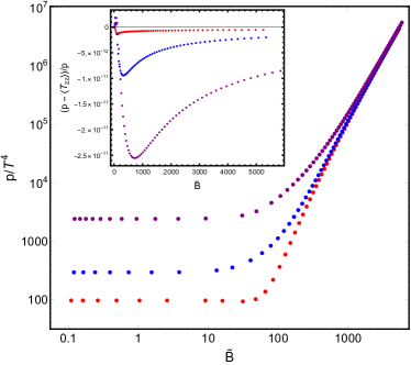
Figure 1: The dimensionless pressure $p/T^{4}$ as a function of the magnetic field $\tilde{B}=B/T^{2}$ for $\gamma=2/\sqrt{3}$ and three different values of $\tilde{\mu}$, namely $\tilde{\mu}=0$ (red), $\tilde{\mu}=4$ (blue), $\tilde{\mu}=10$ (purple). Inset: Difference between $p$ and $\langle T_{zz}\rangle$ which serves as a check of the numerics.

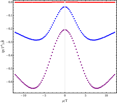
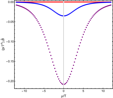
Figure 2: The dimensionless magnetization $(p/T^{4})_{,\tilde{B}}$ as a function of $\tilde{\mu}=\mu/T$ for $\gamma=2/\sqrt{3}$ (left figure) and $\gamma=0$ (right figure). The different curves correspond to magnetic fields $B/T^{2}=\{0.05,12.5,30\}$ (red, blue, purple).

Next, we determine the thermodynamic transport coefficients $M_{i}$ with $i=1,\dots,5$ in this holographic model using the Kubo formulas (30) and (32). From the correlation functions within the Kubo formulas using dimensional analysis we then read off that $M_{1,3,5}$ have dimension of temperature (or chemical potential), while $M_{2}$ has dimension of inverse temperature. Finally, $M_{4}$ is dimensionless.

Magneto-vortical susceptibility $M_{5}$

First, we study the thermodynamic coefficient $M_{5}$ which is also known as magneto-vortical susceptibility and has energy dimension one. We consider the dimensionless combination $M_{5}/T$. We numerically confirm that in both cases for $\gamma$, the magneto-vortical susceptibility $M_{5}/T$ is non-vanishing for nonzero magnetic field and/or nonzero chemical potential. Moreover, as expected and as evident from Figure 3, $M_{5}/T$ is an anti-symmetric function of the chemical potential $\tilde{\mu}$.

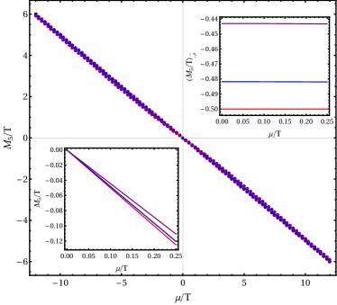
Figure 3: The dimensionless magneto-vortical susceptibility $M_{5}/T$ as a function of the chemical potential $\mu/T$ for $\gamma=2/\sqrt{3}$ (left subfigure) and $\gamma=0$ (right subfigure). The different curves correspond to magnetic fields $B/T^{2}=\{0.05,12.5,30\}$ (red, blue, purple).

Note that the left and right panel of Figure 3 correspond to the case $\gamma=2/\sqrt{3}$ (left panel) and to the case $\gamma=0$ (right panel), respectively. We first discuss the case $\gamma=0.$ For vanishing magnetic field $\tilde{B}=0$ we find a linear relation between $M_{5}/T$ and $\tilde{\mu}$ (at least for the values of the axial chemical potential displayed) of the form $M_{5}/T=-\tilde{\mu}/2$ which is in agreement with Bu:2019qmd . However for finite magnetic fields, $M_{5}/T$ is no longer directly proportional to $\mu/T$ as evident from the inset in the lower left corner. In fact, we numerically find that

$$\frac{\partial(M_{5}/T)}{\partial\tilde{\mu}}\Big{|}_{\tilde{\mu}=0}=-\frac{1}{2}+c\tilde{B}^{2}$$ (138)

where $c$ is a positive constant. If we evaluate $\partial(M_{5}/T)/\partial\tilde{\mu}$ at non-vanishing (but small) chemical potential $\tilde{\mu}$ there are additional corrections to the right hand side of eq. (138).

In case of $\gamma=2/\sqrt{3}$ the thermodynamic coefficient $M_{5}/T$ transitions through zero at a finite value of $\tilde{\mu}$ as opposed to the case $\gamma=0$ where $M_{5}/T$ is decreasing monotonically with increasing chemical potential. In particular, for $\tilde{B}=0$, the relation $M_{5}/T=-\tilde{\mu}\,T/2$ does not longer hold for finite values of the chemical potential $\tilde{\mu}$. This can be seen from the inset in the lower left corner of the right panel of figure 3. For finite but small magnetic fields, there will be again corrections To be more precise we numerically verified the relation (138) for sufficiently small $\tilde{B}$. However, the constant $c$ is negative in contrast to the case in which $\gamma=0$.

Thermodynamic coefficient $M_{2}$

Let us turn to the thermodynamic coefficient $M_{2}$ which has inverse energy dimension, hence we consider the dimensionless combination $M_{2}\cdot T$. We here determine this transport coefficient for the first time in holography. In fact, $M_{2}$ vanishes in the holographic Einstein-Maxwell model, i.e. for the case $\gamma=0$. Hence, in figure 4 we only present results for $\gamma=2/\sqrt{3}$.

Figure 4: The dimensionless thermodynamic susceptibility $M_{2}T$ as a function of the chemical potential $\mu/T$ for $\gamma=2/\sqrt{3}$. The different curves correspond to magnetic fields $B/T^{2}=\{0.05,12.5,30\}$ (red, blue, purple).

As expected, $M_{2}T$ is an odd function of the chemical potential $\tilde{\mu}.$ For small chemical potential $\tilde{\mu}<0.25$ we approximately find a linear proportionality between $M_{2}T$ and $\tilde{\mu}$ as evident from the inset in the lower right corner of figure 4, implying $M_{2}T=a\,\tilde{\mu}$, where the coefficient $a$ depends on $\tilde{B}$. In fact, the coefficient $a$ is given by $a\approx 0.024$ for vanishing magnetic field which is not related to the chiral anomaly coefficient $C=-\gamma$ in an obvious way. Finally, the value of $M_{2}T$ seems to not be sensitive to $\tilde{B}$ for chemical potentials of order $\tilde{\mu}=7$ or larger – at least for reasonably small magnetic fields $\tilde{B}$ displayed in figure 4.

Remaining thermodynamic coefficient $M_{1},M_{3}$ and $M_{4}$

Next, we turn our attention to the remaining thermodynamic transport coefficients $M_{1},M_{3}$ and $M_{4}.$ As discussed in the section on hydrodynamics there are no Kubo formulas available so far which give us directly one of the thermodynamic transport coefficients $M_{i}$ with $i=1,3,4.$ However, we can evaluate the Kubo relations (32) to numerically determine $M_{4,\tilde{\mu}},$ $(M_{1}/T)_{,\tilde{\mu}}$ and $(M_{3}/T)_{,\tilde{\mu}}$ i.e. the derivative of the dimensionless thermodynamic coefficient $M_{i}$ with respect to the chemical potential $\tilde{\mu}.$ It turns out that all these three derivatives vanish numerically. Following the logic of section 2.1.4 we conclude that $M_{4}(\tilde{\mu},\tilde{B})=0$ in our holographic model. A similar conclusion cannot be made for the thermodynamic transport coefficients $M_{1}$ and $M_{3}$. $M_{3}$ is zero due to conformal invariance of theory.

3.3 Results: Dissipationless transport coefficients

In this section we determine the dissipationless transport coefficients in our holographic model which are the Hall conductivity $\tilde{\sigma}_{\perp}$, the Hall viscosities $\tilde{\eta}_{\perp}$ and $\tilde{\eta}_{\parallel}$ as well as the coefficient $c_{10}$ (or alternatively $c_{17}$) which may be interpreted as a shear-induced Hall conductivity.

We first turn our attention to the Hall viscosity $\tilde{\eta}_{\perp}$ which may be computed by the Kubo formula (56f). We find that this transport coefficient vanishes in our holographic model. In fact this is obvious from the gravity side since the relevant fluctuations of the metric, namely $h_{xy}$ and $h_{xx}-h_{yy}$, decouple.

Hall conductivity $\tilde{\sigma}_{\perp}$

Next, we determine numerically the Hall conductivity $\tilde{\sigma}_{\perp}$. To do so we first employ the Kubo formulas (55) for $\rho_{\perp}$ and $\tilde{\rho}_{\perp}$ and then invert the resistivity matrix to obtain the conductivity matrix which contains the Hall conductivity $\tilde{\sigma}_{\perp}$. The Hall conductivity $\tilde{\sigma}_{\perp}$ has dimension of temperature and hence we consider the dimensionless Hall conductivity $\tilde{\sigma}_{\perp}/T$. Its behaviour for fixed chemical potential as a function of the magnetic field is displayed in figures 5 and 6. The Hall conductivity is nonzero even for vanishing chiral anomaly coefficient $C=-\gamma$ as evident from the right panels of those figures. Moreover, the Hall conductivity is only nonzero for nonzero chemical potential and nonzero magnetic field.

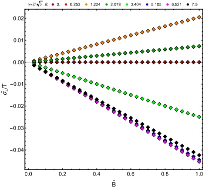
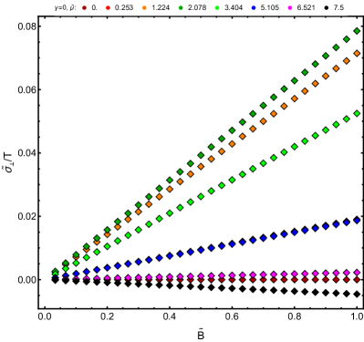
Figure 5: The dimensionless Hall conductivity $\tilde{\sigma}_{\perp}/T$ as a function of a small magnetic field $\tilde{B}$. The left panel shows the case $\gamma=2/\sqrt{3}$, while the right panel displays $\gamma=0$. The different curves correspond to chemical potentials $\tilde{\mu}\in\{0.016,0.253,1.224,2.078,3.404,5.105,6.521,7.5\}$. Note that the specific values of $\tilde{\mu}$ are part of a Chebychev grid in $\tilde{\mu}$ needed to compute the thermodynamic derivatives to high precision. For further reference see appendix B.4.

We first focus on the behavior of the dimensionless Hall conductivity as a function of the magnetic field for fixed chemical potential. As evident from figure 5 the dimensionless Hall conductivity $\tilde{\sigma}_{\perp}/T$ is linear in $\tilde{B}$ for small magnetic fields $\tilde{B}$ and for fixed $\tilde{\mu}$, i.e. $\tilde{\sigma}_{\perp}/T\approx a(\tilde{\mu})\,\tilde{B}.$ The proportionality constant $a(\tilde{\mu})$ displays an interesting behavior as a function of $\tilde{\mu}$ for both values of the chiral anomaly coefficient $C=-\gamma=0$ and $\gamma=2/\sqrt{3}$: first it monotonically increases with increasing chemical potential $\tilde{\mu}$, then turns around and decreases. Finally, the proportionality constant turns negative for even larger values of $\tilde{\mu}$.

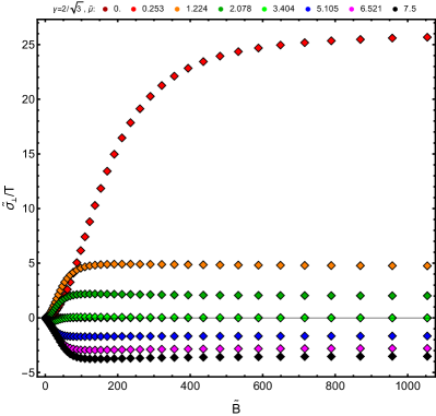
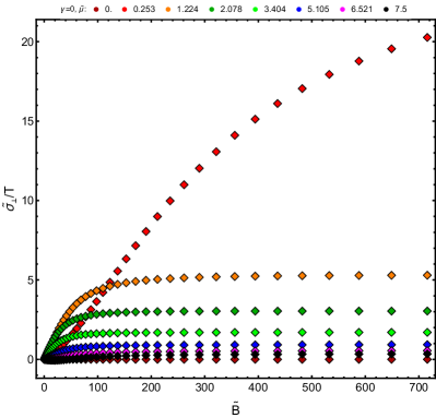
Figure 6: The dimensionless Hall conductivity $\tilde{\sigma}_{\perp}/T$ as a function of a large dimensionless magnetic field $\tilde{B}$. The left panel shows the case $\gamma=2/\sqrt{3}$, while the right panel displays $\gamma=0$.

In addition, the behavior of the dimensionless Hall conductivity for large values of the magnetic field $\tilde{B}$ at fixed chemical potential $\tilde{\mu}$ is displayed in figure 6. The dimensionless Hall conductivity approaches a $\tilde{\mu}$-dependent value for large magnetic fields. Moreover, we may investigate the ratio $\tilde{\sigma}_{\perp}/\sigma_{\perp}$ of the Hall conductivity and the perpendicular conductivity $\sigma_{\perp}$ (the latter one will be discussed in the next subsection) as a function of the magnetic field. For fixed chemical potential $\tilde{\mu},$ the ratio $\tilde{\sigma}_{\perp}/\sigma_{\perp}$ is directly proportional to the magnetic field. This linear relationship persists even for very large values of the magnetic field. The proportionality constant depends on $\tilde{\mu}$ and shows as a function of $\tilde{\mu}$ a behavior similar to that of the proportionality constant $a(\tilde{\mu})$ of the previous paragraph. Specifically, the similarities are that both proportionality constants vanish at $\tilde{\mu}=0$, both increase monotonically with increasing $\tilde{\mu}>0$, reach a maximum value, then decrease monotonically and then turn negative within the range covered by our data.

Hall viscosity $\tilde{\eta}_{\parallel}$ and shear-induced Hall conductivity $c_{10}$

Finally, we investigate the Hall viscosity $\tilde{\eta}_{\parallel}$ and the coefficient $c_{10}$ which may be interpreted as a shear-induced Hall conductivity. Note that both transport coefficients turn out to be zero in case of vanishing chiral anomaly and hence these are novel transport coefficients which are determined here for the first time within a holographic model.

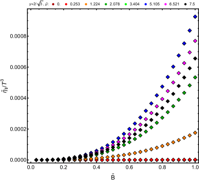
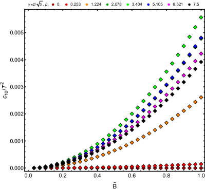
Figure 7: The dissipationless transport coefficients $\tilde{\eta}_{\parallel}/T^{3}$ and $c_{10}/T^{2}$ in presence of the chiral anomaly $\gamma=2/\sqrt{3}$. Without chiral anomaly, both transport coefficients are zero. The green curve with $\tilde{\mu}=3.404$ is hidden under the blue curve.

Figures 7 and 8 display dimensionless versions of the Hall viscosity $\tilde{\eta}_{\parallel}$ and of $c_{10}$ as a function of the magnetic field for fixed chemical potential. Note that the Hall viscosity $\tilde{\eta}_{\parallel}$ has units of temperature $T^{3}$, and hence $\tilde{\eta}_{\parallel}/T^{3}$ is dimensionless. Moreover, $c_{10}$ has the same units as $T^{2}$ implying that $c_{10}/T^{2}$ is dimensionless.

As evident from figures 7 and 8 both dimensionless quantities $\tilde{\eta}_{\parallel}/s$ and $c_{10}/T^{2}$ are only nonzero in the presence of both a non-vanishing magnetic field and a non-vanishing chemical potential. Moreover, note that both quantities are also positive (at least for the magnetic fields and chemical potentials investigated in this paper) even though these quantities are not constrained by the entropy positivity argument from hydrodynamics.

We first investigate the behaviour of the Hall viscosity and the novel shear-induced Hall conductivity for small magnetic fields $\tilde{B}$. As indicated in figure 7 the dimensionless quantities $\tilde{\eta}_{\parallel}/T^{3}$ and $c_{10}/T^{2}$ show the following scaling laws with the magnetic field for fixed chemical potential:

$$\tilde{\eta}_{\parallel}/T^{3}\sim\tilde{B}^{3}\,,\qquad\textrm{and}\qquad c_{10}/T^{2}\sim\tilde{B}^{2}\,.$$ (139)

We defer the plots with the fit curves superimposed, figure 16, to the appendix. The behavior of the corresponding $\tilde{\mu}$-dependent proportionality constants are not very illuminating; both proportionality constants monotonically increase for small chemical potential $\tilde{\mu}$, while they monotonically decrease for larger values of $\tilde{\mu}$.

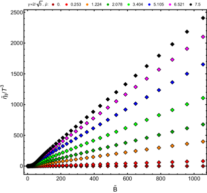
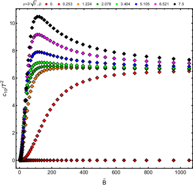
Figure 8: The dissipationless transport coefficients $\tilde{\eta}_{\parallel}/T^{3}$ and $c_{10}/T^{2}$ in presence of the chiral anomaly $\gamma=2/\sqrt{3}$. Without chiral anomaly, both transport coefficients are zero.

Figure 8 displays the dissipationless Hall viscosity and shear-induced Hall conductivity for fixed chemical potential and large magnetic fields. In particular, we find that the dissipationless Hall viscosity is linear in $\tilde{B}$ as shown in the left panel of figure 8. In fact, we find that the proportionality constant between $\tilde{\eta}_{\parallel}/T^{3}$ and $\tilde{B}$ is linear in $\tilde{\mu}$, hence giving us the following universal result for the holographic model considered here:

$$\frac{\tilde{\eta}_{\parallel}}{T^{3}}\approx 0.305\,\tilde{\mu}\,\tilde{B}\,.$$ (140)

Within the full parameter range covered by our numerical data, the above approximation is valid for sufficiently large $\tilde{\mu}\tilde{B}$. The shear-induced Hall conductivity for large magnetic fields $\tilde{B}$ is shown in the right panel of figure 8. It is also tempting to speculate that the novel dimensionless shear-induced Hall conductivity, $c_{10}/T^{2}$, approaches a value for large magnetic fields which is independent of the chemical potential.

3.4 Results: Dissipative hydrodynamic transport coefficients

In this section we investigate the dissipative transport coefficients in our holographic model which may be grouped into

• components of the shear viscosity tensor, namely $\eta_{\perp}$, $\eta_{\parallel}$, $\eta_{1}$ and $\eta_{2}$, as well as the components of the bulk viscosity tensor, namely $\zeta_{1}$ and $\zeta_{2}$,

• dissipative components of the conductivity tensor, namely the longitudinal and perpendicular conductivities $\sigma_{\parallel}$ and $\sigma_{\perp}$,

• novel transport coefficients $c_{4}$ and $c_{5}$, as well as $c_{8}$ which in our model are only nonzero in the presence of a nonzero chiral anomaly coefficient $C=-\gamma\neq 0$, magnetic field $B\neq 0$, and chemical potential $\mu\neq 0$. (In our model $c_{3}=0$ for any values of $\gamma,\,B,\,\mu$.)

Viscosities

We first focus on the various components of the shear viscosity tensor. The perpendicular shear viscosity $\eta_{\perp}$ satisfies $\eta_{\perp}/s=1/(4\pi)$. Note that both $\eta_{\perp}/T^{2}$ and $s/T^{2}$ change as functions of the magnetic field. Remarkably, their functional dependence on $B$ is identical and cancels in the ratio $\eta_{\perp}/s$. This can be shown analytically even in the presence of the chiral anomaly as well as in the presence of $B$ and $\mu$, following Critelli:2014kra .

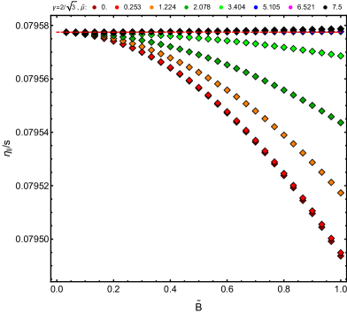
Figure 9: Parallel shear viscosity as function of $\tilde{B}$ for fixed values of $\tilde{\mu}$. The dashed red line indicates the well-known result for $\eta_{\perp}/s$, namely $1/(4\pi).$ Left: $\gamma=2/\sqrt{3}$. For this supersymmetric value of $\gamma$, the ratio of parallel shear viscosity increases with $\tilde{B}$ for $\tilde{\mu}\geq 5$ within the range of parameters displayed here. See figure 10 for a refined statement. Right: $\gamma=0$.

The parallel shear viscosity $\eta_{\parallel}/s$ depends non-trivially on the magnetic field and the chemical potential. The dimensionless parallel shear viscosity $\eta_{\parallel}/s$ is shown in figure 9 for small values of the magnetic field $\tilde{B}$ and in figure 10 for medium and large magnetic fields. It is evident from both figures that $\eta_{\parallel}$ is positive as implied by the hydrodynamic stability analysis. Moreover, for vanishing magnetic field, $\eta_{\parallel}/s$ takes the value $1/(4\pi)$ as expected. Let us first investigate the behavior for small magnetic fields $\tilde{B}$ displayed in figure 9. The dimensionless ratio $\eta_{\parallel}/s$ deviates from $1/(4\pi)$ quadratically, i.e.

$$\frac{\eta_{\parallel}}{s}\sim\frac{1}{4\pi}-c(\tilde{\mu})\tilde{B}^{2}\,,$$ (141)

where $c(\tilde{\mu})$ is a model-dependent coefficient. In fact, $c(\tilde{\mu})$ is positive for vanishing chiral anomaly and monotonically decreases with increasing $\tilde{\mu}$; in contrast, for $\gamma=2/\sqrt{3}$ the coefficient $c(\tilde{\mu})$ turns negative for $\tilde{\mu}>5$. In other words, for those values of $\tilde{\mu}$ the ratio $\eta_{\parallel}/s$ increases for small and intermediate magnetic fields $\tilde{B}$, as evident from the right panel of figure 10. However, for large magnetic fields $\tilde{B}$ the dimensionless parallel shear viscosity $\eta_{\parallel}/s$ decreases monotonically to zero. This is true for both values of the chiral anomaly.

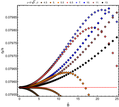
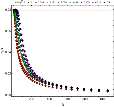
Figure 10: Ratio of parallel shear viscosity and entropy density as function of $\tilde{B}$ with $\gamma=2/\sqrt{3}$; in the left plot the color scheme distinct from right since we use a different set of $\tilde{\mu}$. We observe that $\eta_{\|}/s$ increases initially for $\tilde{\mu}\geq 5$. This behavior is only present with the chiral anomaly. Eventually, all curves tend to zero as displayed in the right figure.

We also investigated whether we can predict the transport coefficient $\eta_{\parallel}/s$ by using horizon data of the charge magnetic black brane. In fact, extending the analysis of Critelli:2014kra we were able to show that this is indeed the case for vanishing chiral anomaly coefficient and in the presence of a magnetic field and a chemical potential. However, in the case of non-vanishing chiral anomaly coefficient we were not able to find an horizon formula for $\eta_{\parallel}/s$.

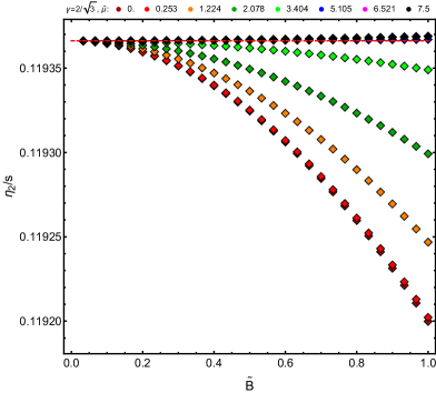
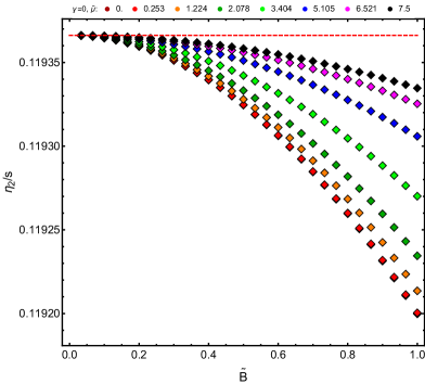
Figure 11: Dimensionless ratio of bulk viscosity $\eta_{2}$ and entropy density for fixed chemical potentials $\tilde{\mu}$. The red dashed line indicates the value for $\eta_{2}/s$ at zero magnetic field, namely $3/(8\pi).$ Note the behavior similar to $\eta_{\parallel}/s$, namely that for $\gamma=2/\sqrt{3}$ there is a distinctly different behavior from the case $\gamma=0$: for the largest three displayed chemical potentials, i.e. for $\tilde{\mu}\geq 5$, the value of the transport coefficient $\eta_{2}/s$ increases with $\tilde{B}$, while it always decreases for $\gamma=0$.

Next, we turn to the dissipative components $\eta_{1}$ and $\eta_{1}$ of the shear viscosity tensor. It suffices to display only $\eta_{2}$ since the bulk viscosity $\zeta_{2}$ vanishes in our holographic model. Hence, the transport coefficients $\eta_{1}$ and $\eta_{2}$ are related by $\eta_{2}=-\frac{1}{3}\eta_{1}$ due to the Onsager relation (65). The behavior of the dimensionless ratio $\eta_{2}/s$ as a function of the magnetic field $\tilde{B}$ is depicted in figure 11. As expected, the ratio $\eta_{2}/s=3/(8\pi)$ for vanishing magnetic field and quadratically deviates from that value for small magnetic fields up to $\tilde{B}=1$. We obtain scaling law similar to the one for $\eta_{\parallel}/s,$ see equation (141). The analogous coefficient $c(\tilde{\mu})$ qualitatively shows the same behavior as in the case of $\eta_{\parallel}/s:$ it monotonically decreases for $\gamma=0$ but stays positive; in contrast for $\gamma=2/\sqrt{3}$ it is not monotonic for the whole range of chemical potentials $\tilde{\mu}$ and even turns negative for intermediate values of $\tilde{\mu}.$

Finally, we numerically checked that the bulk viscosities $\zeta_{1}$ and $\zeta_{2}$ vanish in our model.

Conductivities

Next, we investigate the dissipative components of the conductivity tensor, namely the longitudinal conductivity $\sigma_{\parallel}$ and the perpendicular component $\sigma_{\perp}$. Both quantities have units of temperature, implying that $\sigma_{\perp}/T$ and $\sigma_{\parallel}/T$ are dimensionless. Both dimensionless quantities are almost insensitive to the magnetic field and to $\gamma$. In fact, for both values of the chiral anomaly coefficient and within the range covered by our numerical data, that is $\tilde{\mu}$ between $0$ and $7.5$ $\sigma_{\parallel}/T$ has a relative variation of order $10^{-3}$ for $\tilde{B}<1.$

According to our numerical data, $\sigma_{\perp}/\sigma_{||}$ changes only slightly (at most by $10^{-2}$) in the range $\tilde{B}=0.0,...,1.0$ where our Kubo formula is valid; see derivation in section 2. Due to systematic and numerical errors for this particular ratio it is not possible to consider this change significant. In figure 12 we depict the ratio $\sigma_{\perp}/\sigma_{\parallel}$ which is a measure of the anisotropy of the system. The left panel shows the case $\gamma=2/\sqrt{3}$. Note that in this case the ratio is always larger than one. In contrast, in the case of vanishing chiral anomaly which is shown in the right panel of figure 12 the ratio may be also less than one, depending on the value of the chemical potential. In both cases, i.e. for $\gamma=0$ and for $\gamma=2/\sqrt{3}$ the ratio $\sigma_{\perp}/\sigma_{\parallel}$ deviates from one quadratically in $\tilde{B},$ i.e.

$$\frac{\sigma_{\perp}}{\sigma_{\parallel}}=1+\tilde{c}(\tilde{\mu})\,\tilde{B}^{2}\,,$$ (142)

which holds up to magnetic fields of order $\tilde{B}=1.$

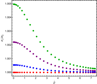
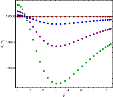
Figure 12: The ratio of longitudinal and perpendicular conductivity $\sigma_{\perp}/\sigma_{||}$ as function of $\tilde{\mu}$ at fixed $\tilde{B}$ for $\gamma=2/\sqrt{3}$ (left) and $\gamma=0$ (right). Each color corresponds to a fixed value of $\tilde{B}$ given by $\tilde{B}=\{1/30,1/3,2/3,1\}$ (red, blue, purple, dark green).

Novel transport coefficients $c_{3}$, $c_{4}$ and $c_{5}$ as well as $c_{8}$

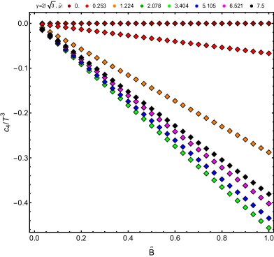
Figure 13: The transport coefficient $c_{4}/T^{3}$ in presence of the chiral anomaly $\gamma=2/\sqrt{3}$. Without chiral anomaly or for vanishing chemical potential, the transport coefficients is zero.

The novel transport coefficients $c_{4}$, $c_{5}$ as well as $c_{8}$ are nonzero in our holographic model. However, they vanish if either the anomaly is absent, i.e. if $\gamma=0$, or if the magnetic field vanishes, or if the chemical potential vanishes. In other words, our holographic calculation is the first to reveal these transport coefficients, because they need $\mu\neq 0$, $B\neq 0$, and the chiral anomaly coefficient $C=-\gamma\neq 0$ simultaneously. Our numerical data shows that $c_{3}$ vanishes in our model. This is expected due to the conformal invariance of theory. The vanishing of $c_{3}$ implies that $c_{4}=-c_{5}/3$ due to the Onsager relation (65). The two relations $c_{4}=-\frac{1}{3}c_{5}$ and $\eta_{2}=-\frac{1}{3}\eta_{1}$ explain why the bound $\det M\geq 0$ with $M$ given by eq. (71) is saturated (within numerical accuracy $\det M\approx 10^{-6}$). The Onsager relation for $c_{4}$ and $c_{5}$ is satisfied up to errors of order $10^{-16}$ at worst ($\tilde{B}=1$, and $\tilde{\mu}=2.078$ corresponding to the dark green curve). We hence plot only the dimensionless quantity $c_{4}/T^{3}$, see figure 13. It turns out that $c_{4}$ is negative which in turn implies that $c_{5}$ is positive. Furthermore, we find $c_{4}/T^{3}\sim d(\tilde{\mu})\tilde{B}$, where $d(\tilde{\mu})$ is negative. Note that $d(\tilde{\mu})$ first decreases as a function of the chemical potential $\tilde{\mu}$ and then increases again. The dimensionless quantity $c_{8}/T^{2}$ as a function of $\tilde{B}$ is depicted in figure 14. Note that $c_{8}/T^{2}$ is proportional to $\tilde{B}$ for small $\tilde{B}$, i.e. the slope changes its sign. Finally, as observed in the other transport coefficients above, $c_{8}/T^{2}$ seems to go to zero for large magnetic fields.

We make the observation that many of the dissipative transport coefficients vanish at large magnetic fields. This may be interpreted as dissipation being suppressed at large magnetic fields, as indicated for example by $\eta_{||}$, see figure 11. A subset of the current authors has previously observed this behavior in the sound attenuation coefficient and the shear diffusion coefficient Ammon:2016fru ; Ammon:2017ded computed in the holographic model we also consider here.

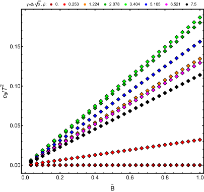
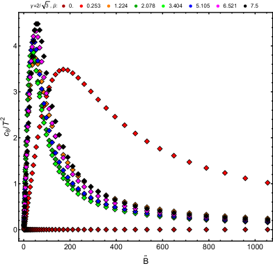
Figure 14: The transport coefficient $c_{8}/T^{3}$ for small and large magnetic fields in presence of the chiral anomaly $\gamma=2/\sqrt{3}$. Without chiral anomaly or for vanishing chemical potential, the transport coefficients is zero.

4 Discussion

In this paper we have used effective field theory methods in order to construct a hydrodynamic description of chiral charged relativistic fluids subject to a strong external magnetic field. In particular, hydrodynamic constitutive relations are generated for the energy-momentum tensor, consistent, and covariant (axial) charge currents. All the independent transport coefficients appearing in the constitutive equations are summarized and classified in tables 3 (thermodynamic), 4 (hydrodynamic, non-dissipative), and 5 (hydrodynamic, dissipative). A discussion and physical interpretation of these transport coefficients is provided in section 2.5.1. Instead of repeating the discussions already given above, in the following we highlight novel phenomena and interesting observations. Novel coefficients and transport effects arise due to the combination of magnetic field, axial charge, and chiral anomaly. These three quantities break time-reversal symmetry, rotational symmetry from $O(3)$ down to $O(2)$, parity symmetry, and chiral symmetry. This symmetry breaking has a drastic impact on the effective field theory description, leading to odd transport effects.

Remarkably, one novel non-dissipative hydrodynamic transport coefficient is found: the shear-induced Hall conductivity $c_{10}$. This transport effect falls into the same category as the known Hall viscosity $\tilde{\sigma}_{\perp}$ and the transverse Hall viscosity $\tilde{\eta}_{\perp}$. This is because all three of them describe time-dependent but dissipationless transport effects. There exists no longitudinal Hall conductivity.

In addition, three novel dissipative transport coefficients are found: the shear-induced conductivity $c_{8}$, as well as the expansion-induced longitudinal conductivities $c_{4}$ and $c_{5}$. Even the well-known charge conductivity and resistivity highlight the drastic changes to the fluid description. In standard hydrodynamic Kubo formulas the charge conductivity is the transport coefficient appearing in the lowest order of the current-current correlator. However, here the lowest transport coefficient is the charge resistivity, see e.g. eq. (54b). The four novel coefficients, $c_{4}$, $c_{5}$, $c_{8}$ and $c_{10}$ can be nonzero in a strong magnetic field if either a chiral anomaly or an axial chemical potential is breaking the parity symmetry.

Kubo relations are derived for 8 independent thermodynamic ($M_{2},\,M_{5}$, $\xi$, $\xi_{B}$, $\xi_{T}$, $M_{1}$, $M_{3}$, $M_{4}$), for 4 independent non-dissipative hydrodynamic ($\tilde{\eta}_{\perp}$, $\tilde{\eta}_{||}$, $c_{10}$, $\tilde{\sigma}_{\perp}$), and for 10 independent dissipative hydrodynamic ($\eta_{\perp}$, $\eta_{||}$, $c_{8}$, $\sigma_{\perp}$, $\sigma_{||}$, $\eta_{1}$, $\eta_{2}$, $\zeta_{1}$, $c_{4}$, $c_{5}$) transport coefficients. For the explicit formulas refer to the equations listed in the third column in tables 3 (thermodynamic), 4 (hydrodynamic, non-dissipative), and 5 (hydrodynamic, dissipative), respectively. In order to derive the thermodynamic transport effects, a field theory generating functional for time-independent $n$-point functions was constructed, see eq. (16). Five Onsager relations, (57) and (65), are found and can be used for cross-checks in explicit computations of the 19 possible hydrodynamic transport coefficients. Kubo relations for the dependent hydrodynamic transport coefficients ($c_{3}$, $c_{14}$, $c_{15}$, $c_{17}$, $\zeta_{2}$) in a parity-violating microscopic theory (one with a chiral anomaly), are provided in eq. (64a), (62c), and (62d). The coefficients $c_{3},\,c_{4},\,c_{5}$ have counterparts in a theory which does not feature an anomaly but which breaks parity through the axial chemical potential, those are given in (59) and (58).

Most prominently, our work discusses strong magnetic fields. The magnetic field breaks rotation symmetry leading to an anisotropic equilibrium state (in the rest frame of the fluid). Let us summarize here which transport effects newly arise at strong magnetic fields of order $\mathcal{O}(\partial^{0})$, versus the effects appearing already in states with weak magnetic fields of order $\mathcal{O}(\partial)$. Consider the list of all transport coefficients provided in tables 3, 4, and 5. First, some of the first order transport coefficients each split into two distinct coefficients, one for transport perpendicular and the other parallel to the magnetic field: $\eta_{||},\,\eta_{\perp},\,\tilde{\eta}_{||},\,\tilde{\eta}_{\perp},\,\sigma_{||},\,\sigma_{\perp}$ (or equivalently $\rho_{||},\,\rho_{\perp}$), $\tilde{\sigma}_{||}$, and $\tilde{\sigma}_{\perp}$. At weak magnetic field all $\alpha_{||}=\alpha_{\perp}$, where $\alpha$ stands for any transport coefficient within this group, and all tilded coefficients vanish. Second, at strong magnetic field new tensor structures in the constitutive relations give rise to $\eta_{1},\,\eta_{2},\,\zeta_{1},\,\zeta_{2}$. At weak magnetic fields $2/3\,\eta_{2}=-2\eta_{1}=\eta$, $\zeta_{1}=\zeta$, and $\zeta_{2}=0$. Third, two of the chiral conductivities, namely $\xi_{B},\,\xi_{TB}$, are promoted from first order in derivative effects at weak magnetic fields to zeroth order effects at strong magnetic fields. Fourth, all of the $M_{n}$ vanish at weak magnetic field, as seen from the $s_{n}$ in table 1. Finally, all $c_{i}$ with $i\geq 3$ vanish at weak magnetic field, as can be deduced from eq. (42).

Interestingly, we find three incarnations of the Nernst effect. Strikingly, we confirm a previous claim Chernodub:2017jcp , that the standard Nernst coefficient, see (112), is proportional to the conformal anomaly, which in turn is then related to the magnetic susceptibility $\chi_{B}$. In addition, we find a magnetic version of the Nernst effect, see (93), with the magnetic Nernst coefficient related to the perpendicular magnetic vorticity susceptibility $M_{2}$, and a momentum Nernst effect, see (111), with momentum Nernst coefficient related to the magneto-vortical susceptibility $M_{5}$.

As a proof of existence and consistency of this hydrodynamic description of chiral fluids we provide an explicit computation in a holographic model. This model is the well-known $\mathcal{N}=4$ Super-Yang-Mills (SYM) theory minimally coupled to an external axial $U(1)_{A}$ gauge field. In order to probe a charged fluid in a magnetic field, we consider perturbations around charged magnetic black brane solution. A Chern-Simons term yields the desired anomalous (chiral) charge current. We find values for 25 of the transport coefficients, for which we verify the 5 Onsager relations (57) and (65). For the remaining two, $M_{1}$ and $M_{3}$ we find only their derivatives as the hydrodynamic theory gives only Kubo relations for those derivatives. However, as stated in section 2, $M_{3}=0$ in a conformal field theory. Of the 25 computed coefficients 20 are nonzero. In our model the gravitational anomaly is absent, hence all effects associated with $c_{1}$, see eq. (17), vanish in this model. The magneto-acceleration susceptibility $M_{3}$ vanishes due to conformal invariance. Also the transverse Hall viscosity $\tilde{\eta}_{\perp}$ vanishes, however, without any reason obvious to us.

Due to conformal invariance the bulk viscosities $\zeta_{1}$, and $\zeta_{2}$ vanish. In addition, $c_{3}$ is zero.

As discussed in the introduction, we have restricted our attention to an axial $U(1)_{A}$ symmetry in this work. In Nature, however, an interplay between axial and vector symmetries is generic. In the standard model of particle physics, for example, currents of left- and right-handed fermions may be combined into axial and vector currents. Thus, it is natural to extend the hydrodynamic description to the combination, $U(1)_{V}\times U(1)_{A}$. As usual, the vector and axial currents can be related to the current of left- and right-handed particles by $J^{\mu}_{V/A}=(J^{\mu}_{L}\pm J^{\mu}_{R})/2$. A different combination of currents may be interesting in the context of the $\Lambda$-hyperon polarization effect recently discovered in heavy ion collisions STAR:2017ckg : one may consider the helicity current instead of the axial current Ambrus:2019khr ; Ambrus:2020oiw . This would require disentangling the axial current carried by particles from that carried by anti-particles, which is the definition of the helicity current.

A next logical step is to restrict the vector gauge fields to satisfy Maxwell’s equations and allow them to interact dynamically with the fluid. The resulting effective field theory may be labelled magnetohydrodynamics. However, previous constructions excluding anomalies Grozdanov:2016ala ; Grozdanov:2016tdf ; Kovtun:2018dvd ; Grozdanov:2017kyl indicate that such a description goes well beyond what is known as textbook magnetohydrodynamics. Although the setting with dynamical gauge fields Grozdanov:2017kyl is distinct from the one we consider here, some of the Kubo relations associated with energy momentum tensor correlators agree with ours. In order to understand this observation, recall that the constitutive equations for hydrodynamics coupled to external electromagnetic fields can be interpreted as those of hydrodynamics coupled to dynamical gauge fields Hernandez:2017mch .

Over the past decade progress has been made towards a generating functional yielding non-equilibrium contributions to the constitutive relations and more generally to the $n$-point functions Jensen:2012jh ; Crossley:2015evo ; Haehl:2015pja ; Haehl:2015foa ; Haehl:2016pec ; Haehl:2018lcu ; Glorioso:2018wxw . This progress will eventually establish hydrodynamics as an effective field theory. Our work provides a step towards this goal by encoding the equilibrium response in our generating functional (16). Extending it to include non-equilibrium transport effects would be accomplishing that goal. In order to understand the fluid response to time-dependent or spatially modulated sources, frequency and wave length dependence of the transport coefficients should be studied, which can be computed with our methods. In the holographic context frequency- and wavelength-dependent transport coefficients have been computed before Amado:2011zx ; Hoyos2013 . One may also venture to extend hydrodynamics in strong electromagnetic fields to descriptions of fluids far-from-equilibrium. Recent developments applying insights from resurgence are promising in this regard Romatschke:2017vte ; Heller:2013oxa ; Heller:2015dha ; Heller:2020anv ; Heller:2020uuy . For an alternate expansion, linearizing in hydrodynamic fields, see Bu:2016oba ; Bu:2016vum ; Bu:2018drd ; Bu:2018psl ; Bu:2019mow .

An application of our fluid description is the hydrodynamic modelling of heavy ion collisions Romatschke:2017ejr , as well as the hydrodynamic description of astrophysical fluids in strong magnetic fields RezzollaHydroTextbook ; Joyce:1997uy ; Boyarsky:2011uy ; Tashiro:2012mf ; Brandenburg:2017rcb (see Boyarsky:2020ani ; Boyarsky:2020cyk for recent papers), and the description of condensed matter materials and cold atom gases subjected to magnetic fields, see Fujita:2012fp ; An:2020tkn ; Hoyos:2020ywe ; Baggioli:2020edn for holographic models in this context. While these systems are subject to a strong dynamical vector magnetic field, when the backreaction of the fluid on the electromagnetic field can be neglected, the description in terms of external magnetic fields as outlined in this paper may be useful. For example this is the case in (quantum) Hall effect experiments, ultracold atom gases in strong magnetic field traps, and possibly intermediate time phase of heavy-ion-collisions where the magnetic field changes from growing to decaying.

Moreover, external axial gauge fields are of importance in the context of Weyl semimetals. Elastic deformations therein couple to the fermionic low-energy excitations with different signs, giving rise to effective axial gauge fields Cortijo_2015 ; Cortijo:2016wnf . Such deformations naturally arise at the surfaces of Weyl semimetals, inducing localised axial magnetic fields in their vicinity. In fact, the surface states (so-called Fermi arcs) may be understood from this perspective in terms of lowest Landau levels generated by those axial magnetic fields (see e.g. Chernodub:2013kya ; Ammon:2016mwa ).

In quantum chromodynamics (QCD) the chiral magnetic effect and more generally QCD thermodynamics in the presence of an external magnetic field has been investigated using lattice simulations Buividovich:2009wi ; Buividovich:2010tn ; Bali:2011qj ; Bali:2012zg ; Bali:2014kia ; Astrakhantsev:2019zkr . In particular, a result from lattice gauge theory gives motivation to the study of holographic models as a surrogate for QCD with strong magnetic fields: the magnetoresponse of $\mathcal{N}=4$ SYM as computed in the same holographic dual we used in this work has been found to have universal similarities to the magnetoresponse of QCD Endrodi:2018ikq . The Kubo relations for thermodynamic transport coefficients and constitutive relations derived in the present paper facilitate a more detailed comparison of the equilibrium response in QCD and SYM subject to external magnetic fields.

The time-evolution of (electro)magnetic fields in relativistic heavy-ion-collisions has also been considered Voronyuk:2011jd ; Inghirami:2019mkc . It would be interesting to compare the hydrodynamic transport in our holographic model to the results from these other approaches. Even an analysis of the data from the other approaches using our Kubo relations may lead to interesting results in and out of equilibrium.

Especially with regard to condensed matter physics, we predict additional effects in the Hall response of materials. Hall effects of quantum or classical nature have been studied in condensed matter physics since Hall’s discovery in 1879.

For example, Hall viscosity Avron:1995fg ; Avron:1997 is a dissipationless transport coefficient of relevance to topological states of matter, e.g. fractional quantum Hall systems, see for example Wen:2017 ; Hoyos:2014pba . In (2+1) dimensions Hall viscosity in a hydrodynamic context has been found to be given by the angular momentum density in condensed matter Read:2008rn ; Read:2010epa , and in holographic systems, e.g. in application to $p$-wave superfluids Son:2013xra . In fractional quantum Hall systems the Hall viscosity is quantized and may be used to detect topological phase transitions Hoyos:2014pba .

However, the Hall viscosities which we find in (3+1) dimensions prepared in an anisotropic state are novel. We predict two distinct Hall viscosities, one associated with the plane parallel to a strong magnetic field, the other with a plane perpendicular to it with generically distinct values. It would be very interesting to understand how the anomalous Hall effect Nagosa2010 may fit into our hydrodynamic description. We assume that it would be measured in our Hall conductivity $\tilde{\sigma}_{\perp}$. Potentially analogous effects may appear in the other Hall coefficients. Finally, the novel dissipationless coefficient $c_{10}$ is to be interpreted as a Hall response of a charge current to the shear of a fluid in a plane in the fluid creates a charge current perpendicular to that plane. This considerably extends the possibilities for Hall physics to be studied in the future and promises new technological applications.

One promising testing ground are Weyl- or Dirac-semimetals Nielsen:1983 ; Cortijo_2015 ; Cortijo:2016wnf ; Pikulin:2016 ; Taguchi:2016 ; Breunig:2019kjd ; Zhang:2018 . A quantum Hall effective action for the anisotropic Dirac semimetal is discussed in Hoyos:2020ywe . Experiments with Weyl semimetals report the observation of chiral transport effects in presence of magnetic fields 2014arXiv1412.6543L ; 2015arXiv150606577S ; 2015arXiv150407698Z ; 2015arXiv150600924W ; 2015arXiv150603190Y . In these experiments, the relevant observable is the negative magnetoresistance. However, note that negative magnetoresistance cannot unambigously be related to the presence of a chiral anomaly (see e.g. the holographic computations in Baumgartner:2017kme ; Ammon:2009jt ). Hydrodynamic behavior has been measured most reliably or has been theoretically argued for in (2+1)-dimensional materials Berdyugin162 ; Molenkamp:1994 ; Moll1061 where the parity anomaly leads to anomalous transport effects DiSante:2019zrd ; Tutschku:2020rjq ; Tutschku:2020drw ; parityAnomalyQHEWuerzburgPRL ; Haldane:1988zza . Our discussion of (2+1)-dimensional hydrodynamics in section 2.5.2 will help relating our (3+1)-dimensional hydrodynamic transport effects to these lower dimensional experiments and theoretical descriptions.

All these examples, taken from fields as different as particle physics and condensed matter physics, illustrate the importance of a more detailed understanding of the response of (non)relativistic fluids in the presence of electromagnetic fields and anomalies, towards which this work is taking a step.

coefficient	name	Kubo formulas	$\mathcal{C}$	$\mathcal{P}$	$\mathcal{T}$
Thermodynamic $\left(\lim\limits_{\mathbf{k}\to 0}\lim\limits_{\omega\to 0}\right)$,  non-dissipative
momentum diffusion sector
${M_{2}}$	perp. magnetic vorticity susceptibility	$T^{xz}T^{yz}$ (30)	+	-	+
${M_{5}}$	magneto-vortical susceptibility	$T^{tx}T^{yz}$ (30,31)	+	-	+
$\xi=\xi_{TB}$	chiral vortical conductivity	$J^{x}T^{ty}$ (38,39)	+	+	+
$\xi_{B}$	chiral magnetic conductivity	$J^{x}J^{y}$ (38,39)	+	-	+
$\xi_{T}$	chiral vortical heat conductivity	$T^{tx}T^{ty}$ (38,39)	+	-	+
scalar sector
${M_{1}}$	magneto-thermal susceptibility	$J^{t}T^{xx}$ (32)	+	+	-
${M_{3}}$	magneto-acceleration susceptibility	$J^{t}T^{tt}$ (32)	+	+	-
${M_{4}}$	magneto-electric susceptibility	$J^{t}J^{t}$ (32)	+	-	-

Table 3: Independent thermodynamic transport coefficients in a charged chiral thermal plasma subjected to a strong $U(1)_{A}$ magnetic field. The column “Kubo formulas” points to the equations containing the relevant Kubo formulas. In that column, the operator combinations, e.g. $J_{x}T_{ty}$ indicate the correlation function appearing in the Kubo formula for the spatial momentum to be aligned with the magnetic field. The susceptibilities $\chi_{11}$, $\chi_{13}$, $\chi_{33}$ and $\chi_{B}$ are not counted here as transport coefficients because they are thermodynamic derivatives of pressure. Here, “perp.” denotes “perpendicular”.

Non-dissipative Hydrodynamic $\left(\lim\limits_{\omega\to 0}\lim\limits_{\mathbf{k}\to 0}\right)$
coefficient	name	Kubo formulas	$\mathcal{C}$	$\mathcal{P}$	$\mathcal{T}$
shear sector
${\tilde{\eta}_{\perp}}$	transverse Hall viscosity	$T^{xy}(T^{xx}-T^{yy})\eqref{eq:tildeEtaPerpKubo}$	+	-	+
momentum diffusion sector
$\boxed{c_{10}}\propto c_{17}$	shear-induced Hall cond.	$T^{tx}T^{xz},T^{tx}T^{yz}$ (61,62a,62b)	+	+	+
${\tilde{\eta}_{||}}$	parallel Hall viscosity	$T^{yz}T^{xz}$ (60b)	+	-	+
${\tilde{\sigma}_{\perp}}$	Hall conductivity	$J^{x}J^{x}$,$J^{x}J^{y}$ (55,54b,54c)	+	-	+

Table 4: Independent non-dissipative hydrodynamic transport coefficients in a charged chiral thermal plasma subjected to a strong $U(1)_{A}$ magnetic field. Similar to table 3. Note that the Hall conductivity $\tilde{\sigma}_{\perp}$ is dissipationless, however, it is computed from the resistivity matrix including $\rho$ and $\tilde{\rho}$, which are both dissipative. Here, “cond.” denotes “conductivity”. Boxed quantities are novel in this paper.

dissipative, hydrodynamic $\left(\lim\limits_{\omega\to 0}\lim\limits_{\mathbf{k}\to 0}\right)$
coefficient	name	Kubo formulas	$\mathcal{C}$	$\mathcal{P}$	$\mathcal{T}$
shear sector
$\eta_{\perp}$	perp. shear viscosity	$T^{xy}T^{xy}$ (2.2.4)	+	+	-
momentum diffusion sector
${\eta_{||}}$	parallel shear viscosity	$T^{xz}T^{xz}$ (60a)	+	+	-
$\boxed{c_{8}}\propto c_{15}$	shear-induced conductivity	$T^{tx}T^{xz}$, $T^{tx}T^{yz}$ (58)	+	+	+
${\rho_{\perp}}$	perp. resistivity	$J^{x}J^{x}$ (55)	+	+	-
$\sigma_{||}$	long. conductivity	$J^{z}J^{z}$ (54a)	+	+	-
$\sigma_{\perp}$	perp. conductivity	$\rho_{ab}\equiv(\sigma^{-1})_{ab}=\rho_{\perp}\delta_{ab}+\tilde{\rho}_{\perp}\,\epsilon_{ab}$	+	+	-
scalar sector
$\eta_{1}$	bulk viscosity	$\mathcal{O}_{1}\mathcal{O}_{1}$ (56c)	+	+	-
$\eta_{2}$	bulk viscosity	$\mathcal{O}_{2}\mathcal{O}_{2}$ (56d)	+	+	-
$\zeta_{1}$	bulk viscosity	$T^{ij}(T^{xx}+T^{yy})$(56a)	+	+	-
$\zeta_{2}$	bulk viscosity	$3\zeta_{2}-6\eta_{1}=2\eta_{2}$	+	+	-
$\boxed{c_{4}}$	expan.-induced long. cond.	$J^{x}T^{xx}$ (58)	+	-	-
$\boxed{c_{5}}\propto c_{14}$	expan.-induced long. cond.	$J^{z}T^{zz}$ (58)	+	-	-
$c_{3}$		$c_{5}=-3(c_{3}+c_{4})$	+	-	-

Table 5: Independent dissipative hydrodynamic transport coefficients in a charged chiral thermal plasma subjected to a strong $U(1)_{A}$ magnetic field. Similar to table 4. Abbreviations: perpendicular (perp.), longitudinal (long.), conductivity (cond.), expansion (expan.). Gray shaded rows display relation of dependent transport coefficients to the set of independent transport coefficients. Boxed quantities are novel in this paper.

Appendix A Details of the hydrodynamic calculation

quantity	${C}$	${P}$	${T}$
$t$	+	+	-
$x^{i}$	+	-	+
$\varrho$	+	+	+
$T,h_{tt},T^{tt}$	+	+	+
$\mu_{A},A_{t},J^{t}$	+	-	+
$\mu_{V},V_{t},J_{V}^{t}$	-	+	+
$A_{i},J^{i}$	+	+	-
$V_{i},J_{V}^{i}$	-	-	-
$A_{\varrho}$	+	-	-
$V_{\varrho}$	-	+	-
$u^{i},h_{ti},T^{ti}$	+	-	-
$h_{ij},T^{ij}$	+	+	+
$B^{i}$	+	-	-
$B_{V}^{i}$	-	+	-
$E^{i}$	+	+	+
$E_{V}^{i}$	-	-	+
$dx^{\mu}\wedge dx^{\nu}\wedge dx^{\rho}\wedge dx^{\sigma}\wedge dx^{\kappa}$	+	-	-
$\int\limits_{i}^{f}A\wedge F\wedge F$	+	+	+
$\int\limits_{i}^{f}V\wedge F_{V}\wedge F_{V}$	-	-	+
$u^{t}$	+	+	+
generating functionals $W_{s},\,W_{cons},\,W_{cov}$ (axial $U(1)_{A}$)	+	+	+

Table 6: Transformation properties of the following quantities under charge-parity ${C}$, parity ${P}$, and time-reversal ${T}$: field theory coordinates $x^{\mu}=t,\,x,\,y,\,z$, field theory axial $U(1)_{A}$ (or vector $U(1)_{V}$) current $J^{\mu}$ (or $J^{\mu}_{V}$) and energy-momentum tensor $T^{\mu\nu}$, hydrodynamic variables $T,\,u^{\mu},\,\mu$ (or $\mu_{V}$) and sources $h_{\mu\nu}$, $A_{\mu}$ (or $V_{\mu}$), as well as the extra spatial direction $r$ and Chern-Simons term, both appearing in the anomaly inflow formulation in section 2. In some entries we have split the time $t$ from the spatial components in the field theory directions, labeled by $i=x,\,y,\,z$, and the $\varrho$-component. Note that we consider here an axial gauge field $A_{\mu}$ which has transformation properties distinct from that of a vector gauge field. We here refer to the parity ${P}$ with respect to the field theory directions $x,\,y,\,z$. The integral boundaries are indicated as initial, $i$, and final, $f$.

A.1 Consistent-consistent Kubo Formulas

The Kubo formulas in sections 2.1 and 2.2.4 were written in terms of covariant-consistent correlation functions. The consistent-consistent connected correlation functions are the same as the covariant-covariant connected correlation functions since

$$\langle J^{\mu}_{cov}J^{\nu}_{cov}\rangle = \langle(J^{\mu}_{cons}+J^{\mu}_{BZ})(J^{\nu}_{cons}+J^{\nu}_{BZ})\rangle$$ (143)

$$= \langle J^{\mu}_{cons}J^{\nu}_{cons}\rangle+J^{\mu}_{BZ}\langle J^{\nu}_{cons}\rangle+\langle J^{\mu}_{cons}\rangle J^{\nu}_{BZ}+J^{\mu}_{BZ}J^{\nu}_{BZ}\,,$$

and the last three terms are disconnected. The consistent-consistent connected correlation functions differ from the covariant-consistent connected correlation functions (63) by the variation of the Bardeen-Zumino polynomial

$$G_{J_{cons}^{\mu}J_{cons}^{\nu}}=G_{J_{cov}^{\mu}J_{cons}^{\nu}}+\frac{\delta J^{\mu}_{BZ}}{\delta A_{\nu}}\,.$$ (144)

Alternatively, the static consistent-consistent correlation functions can be found by varying the 3+1 dimensional generating functional (16)

$$G_{J_{cons}^{\mu}J_{cons}^{\nu}}(\omega=0,\mathbf{k})=\frac{\delta^{2}W_{cons}}{\delta A_{\mu}(\mathbf{k})\delta A_{\nu}(-\mathbf{k})}\,.$$ (145)

The Kubo formula for $\xi_{B}$ in terms of static consistent-consistent correlation functions is then

$$\langle J^{x}_{cons}(\mathbf{k})J^{z}_{cons}(-\mathbf{k})\rangle=-ik_{y}(\xi_{B}-{\textstyle{\frac{1}{3}}}CA_{t})\,,$$ (146a)

for fluctuations perpendicular to the magnetic field and

$$\langle J^{x}_{cons}(\mathbf{k})J^{y}_{cons}(-\mathbf{k})\rangle=-ik_{z}(\xi_{B}-{\textstyle{\frac{1}{3}}}CA_{t})\,,$$ (146b)

for fluctuations parallel to the magnetic field. These thermodynamic formulas are unchanged by the presence of strong magnetic fields, and agree with the expressions found in Amado:2011zx ; Jensen:2013vta . We can also rewrite the current-current Kubo formulas in  (64a) in terms of the consistent currents

$${\textstyle{\frac{1}{\omega}}}{\rm Im}\,G_{J^{z}_{cons}J^{z}_{cons}}(\omega,{\bf k}{=}0)=\sigma_{\parallel}+\cdots\,,$$ (147a)

$${\textstyle{\frac{1}{\omega}}}{\rm Im}\,G_{J_{cons}^{x}J^{x}_{cons}}(\omega,{\bf k}{=}0)=\omega^{2}\rho_{\perp}\frac{w_{0}(w_{0}-{M_{5}}_{,\mu}B_{0}^{2})}{B_{0}^{4}}\,,$$ (147b)

$${\textstyle{\frac{1}{\omega}}}{\rm Im}\,G_{J_{cons}^{x}J_{cons}^{y}}(\omega,{\bf k}{=}0)=\frac{n_{0}}{B_{0}}-\omega^{2}\tilde{\rho}_{\perp}\frac{w_{0}(w_{0}-{M_{5}}_{,\mu}B_{0}^{2})}{B_{0}^{4}}\,{\rm sign}(B_{0})\,,$$ (147c)

$${\textstyle{\frac{1}{\omega}}}{\rm Im}\,G_{J_{cons}^{z}O_{1}}(\omega,{\bf k}{=}0)=-c_{4}\,{\rm sign}(B_{0})+\cdots\,,$$ (147d)

$${\textstyle{\frac{1}{\omega}}}{\rm Im}\,G_{J_{cons}^{z}O_{2}}(\omega,{\bf k}{=}0)=-c_{5}\,{\rm sign}(B_{0})+\cdots\,$$ (147e)

$${\textstyle{\frac{1}{\omega}}}\delta_{ij}{\rm Im}\,G_{T^{ij}J_{cons}^{z}}(\omega,{\bf k}{=}0)=3c_{3}\,{\rm sign}(B_{0})+\cdots\,,$$ (147f)

$${\textstyle{\frac{1}{\omega}}}{\rm Im}\,G_{O_{2}J_{cons}^{z}}(\omega,{\bf k}{=}0)=2c_{14}\,{\rm sign}(B_{0})+\cdots\,,$$ (147g)

where $O_{2}$ is defined below equation (2.2.4). The terms omitted vanish for $B_{0}\ll T_{0}^{2}$ or when $M_{1}=M_{3}=M_{4}=0$.

A.2 Eigenmodes

In this appendix, we give more details about the gapless eigenmodes found in section 2.4.

The velocities $v_{0}\,,\ v_{+}$ and $v_{-}$ appearing in eq. (79) are the solutions to the cubic equation

$$a_{3}v^{3}+a_{2}v^{2}+a_{1}v+a_{0}=0\,,$$ (148)

where

$$a_{0}=-B_{0}C\frac{(s_{0}T_{0})^{2}}{\det(\chi)}\,,$$

$$a_{1}=v_{s}^{2}-\frac{(B_{0}C\mu_{0}T_{0})^{2}}{\det(\chi)}\frac{ds}{dT}\,,$$

$$a_{2}=B_{0}C\left(\frac{\mu_{0}^{2}}{w_{0}}-2n_{0}\mu_{0}\frac{\chi_{11}-\mu_{0}\chi_{13}}{{\rm det}(\chi)}+w_{0}\frac{\chi_{11}-\mu_{0}^{2}\chi_{33}}{{\rm det}(\chi)}\right)\,,$$

$$a_{3}=-1+\frac{(B_{0}C\mu_{0}T_{0})^{2}}{\det(\chi)}\frac{ds}{dT}\,,$$

and the speed of sound expressed in terms of the elements of the susceptibility matrix is given by (78)

These can be solved perturbatively in $B_{0}C$. We first label

$$\alpha =\frac{(s_{0}T_{0})^{2}}{{\rm det}(\chi)}\,,\quad\quad\quad\quad\beta=\frac{(\mu_{0}T_{0})^{2}}{{\rm det}(\chi)}\frac{ds}{dT}\,,$$

$$\gamma =\frac{\mu_{0}^{2}}{w_{0}}-2n_{0}\mu_{0}\frac{\chi_{11}-\mu_{0}\chi_{13}}{{\rm det}(\chi)}+w_{0}\frac{\chi_{11}-\mu_{0}\chi_{33}}{{\rm det}(\chi)}\,,$$

from which we find

$$v_{0} =B_{0}C\frac{\alpha}{v_{s}^{2}}+\cdots\,,$$ (149)

$$v_{\pm} =\pm v_{s}+B_{0}C\frac{\gamma v_{s}^{2}-\alpha}{2v_{s}^{2}}\mp B_{0}^{2}C^{2}\frac{3\alpha^{2}-2\alpha\gamma v_{s}^{2}+v_{s}^{4}(4\beta(1-v_{s}^{2})-\gamma^{2})}{8v_{s}^{5}}+\cdots\,,$$

where we have omitted terms of order $B_{0}^{3}C^{3}$ and higher.

The damping coefficient in eq. (82) has the following corrections

$$\frac{w_{0}}{W_{0}} =1+CB_{0}\frac{\chi_{11}w_{0}+2n_{0}\mu_{0}(\mu_{0}\chi_{13}-\chi_{11})+\mu_{0}^{2}\left((3\det(\chi)-\chi_{13}^{2}w_{0})/\chi_{11}-\det(\chi)/w_{0}\right)-(s_{0}T_{0}/v_{s})^{2}}{v_{s}\det(\chi)}\,,$$ (150)

$$\quad\quad\quad\Sigma_{\perp}=\frac{8\mu_{0}w_{0}^{2}(\mu_{0}\chi_{13}-\chi_{11})(w_{0}\chi_{13}-n_{0}\chi_{11})}{v_{s}(n_{0}\chi_{11}-2w_{0}\chi_{13})^{2}\det(\chi)}\,,$$

and $\Sigma_{\parallel}$ is a lengthy function of the susceptibilities, other thermodynamic derivatives of the pressure, the chemical potential and the temperature. We have omitted higher order terms in $CB_{0}$ in eq. (82).

The leading correction to the longitudinal diffusion constant in eq. (84) is

$$D_{\parallel}=\frac{w_{0}^{2}\sigma_{\parallel}}{v_{s}^{2}\det(\chi)}+B_{0}^{2}C^{2}\left(\left(\frac{ds}{d\mu}\right)_{p}\frac{s_{0}^{4}T_{0}^{6}}{3v_{s}^{6}{\rm det}(\chi)^{3}}(3\zeta_{1}+10\eta_{1}+6\eta_{2})+F\sigma_{\parallel}\right)+\cdots\,,$$

where $\left(\frac{ds}{d\mu}\right)_{p}$ is the derivative keeping pressure and magnetic field fixed, and

$$F =\frac{s_{0}^{4}\,T_{0}^{6}\,w_{0}}{v_{s}^{8}\,{\rm det}(\chi)^{4}}\Bigg{[}2\left(\frac{dn}{d\mu}\right)_{p}^{2}s_{0}^{2}\mu_{0}^{2}+2\left(\frac{ds}{d\mu}\right)_{p}^{3}n_{0}T_{0}\mu_{0}^{2}$$

$$+\left(\frac{ds}{d\mu}\right)_{p}^{2}\left(3s_{0}^{2}T_{0}^{2}-2\left(\frac{dn}{d\mu}\right)_{p}s_{0}T_{0}\mu_{0}^{2}-\mu_{0}^{2}n_{0}\left(n_{0}-2\left(\frac{dn}{d\mu}\right)_{p}\mu_{0}\right)\right)$$

$$+2\left(\frac{dn}{d\mu}\right)_{p}\left(\frac{ds}{d\mu}\right)_{p}s_{0}\mu_{0}\left(3s_{0}T_{0}+\mu_{0}\left(n_{0}-\left(\frac{dn}{d\mu}\right)_{p}\mu_{0}\right)\right)\Bigg{]}\,.$$

The positivity of the diffusion constant implies $\sigma_{\parallel}>0$.

A.3 A comment on magnetic susceptibilities

In this appendix, we comment on the choice of naming ${\chi_{B}}=2p_{,B^{2}}$ as magnetic susceptibility. The thermodynamic function ${\chi_{B}}$ appears in the constitutive relation for the magnetic polarization in front of $B^{\mu}$. To be more precise, we can define $\delta W=\frac{1}{2}\int\sqrt{-g}M^{\mu\nu}\delta F_{\mu\nu}=\int\sqrt{-g}\left(m^{\mu}\delta B_{\mu}+p^{\mu}\delta E_{\mu}\right)$ (see Kovtun:2016lfw ). The polarization tensor $M_{\mu\nu}$ is related to the polarization and magnetization vectors $p_{\mu}$ and $m_{\mu}$ by

$$M_{\mu\nu}=p_{\mu}u_{\nu}-p_{\nu}u_{\mu}-\epsilon_{\mu\nu\rho\sigma}u^{\rho}m^{\sigma}\,.$$ (151)

Varying the generating functional $W=\!\int\sqrt{-g}{\cal F}(T,\mu,B^{2},E^{2},B{\cdot}E,B{\cdot}a,B{\cdot}\Omega,E{\cdot}a,E{\cdot}\Omega,\cdots)$ we find the constitutive relations for $p^{\mu}$ and $m^{\mu}$

$$m^{\mu}=2{\cal F}_{,B^{2}}B^{\mu}+{\cal F}_{,B{\cdot}E}E^{\mu}+{\cal F}_{,B{\cdot}a}a^{\mu}+{\cal F}_{,B{\cdot}\Omega}\Omega^{\mu}+\cdots\,,$$ (152)

$$p^{\mu}=2{\cal F}_{,E^{2}}E^{\mu}+{\cal F}_{,B{\cdot}E}B^{\mu}+{\cal F}_{,E{\cdot}a}a^{\mu}+{\cal F}_{,E{\cdot}\Omega}\Omega^{\mu}+\cdots\,.$$

Now, if we focus on the zeroth order constitutive relations and with strong magnetic fields so that $B^{\mu}={\cal O}(1)$ while $E^{\mu}=a^{\mu}=\Omega^{\mu}={\cal O}(\partial)$, we simply find

$$m^{\mu}=2p_{,B^{2}}B^{\mu}+\cdots\,,\quad p^{\mu}=\cdots\,,$$ (153)

that is, the thermodynamic function relating $B^{\mu}$ to $m^{\mu}$ is simply $2p_{,B^{2}}$. When written in terms of magnetic field strength $H^{\mu}=B^{\mu}-m^{\mu}$, the relation reads

$$m^{\mu}=\frac{2p_{,B^{2}}}{1-2p_{,B^{2}}}H^{\mu}\,.$$ (154)

However, if we are interested in seeing how the magnetization changes as we change the magnetic field $\delta m^{\mu}=m^{\mu\nu}\delta B_{\nu}$, we find

$$m^{\mu\nu}=4p_{,B^{2}B^{2}}B^{\mu}B^{\nu}+2p_{,B^{2}}g^{\mu\nu}\,,$$ (155)

where, in particular, the term aligned with $B^{\mu}$ is

$$m^{\mu\nu}B_{\mu}B_{\nu}=4p_{,B^{2}B^{2}}B^{4}+2p_{,B^{2}}B^{2}=p_{,BB}B^{2}$$ (156)

where $B=\sqrt{B^{2}}$. This is often quoted as the magnetic susceptibility at finite magnetic field.

Note that the change in magnetization orthogonal to the existing magnetic field is given by $2p_{,B^{2}}$. That is, for

$$\delta B^{\mu}=\delta B^{\mu}_{\parallel}+\delta B^{\mu}_{\perp}\,,$$ (157)

we have the following change in the magnetization

$$\delta m^{\mu}=p_{,BB}\,\delta B^{\mu}_{\parallel}+2p_{,B^{2}}\delta B^{\mu}_{\perp}\,.$$ (158)

This suggests we could call $2p_{,B^{2}}$ the perpendicular magnetic susceptibility and $p_{,BB}$ the parallel magnetic susceptibility.

Appendix B Details of the holographic calculation

In this section, we present more details of the holographic calculation. We also outline the numerical procedure used to construct the numerical solutions in this work and compute the transport coefficients.

B.1 Expansion close to horizon and conformal boundary

Here we include the near-boundary and near-horizon expansions for the functions defined in the metric and gauge field ansatz, eq. (130) and eq. (131), used in the holographic model. The solution close to the conformal boundary (i.e. for $\varrho=0$) reads

$$u(\varrho)=1+\varrho^{4}\left[u_{4}+{\cal O}(\varrho^{2})\right]+\varrho^{4}\ln(\varrho)\left[\frac{B^{2}}{6}+{\cal O}(\varrho^{2})\right]\,,$$

$$v(\varrho)=1+\varrho^{4}\left[-\frac{w_{4}}{2}+{\cal O}(\varrho^{2})\right]+\varrho^{4}\ln(\varrho)\left[-\frac{B^{2}}{24}+{\cal O}(\varrho^{2})\right]\,,$$

$$w(\varrho)=1+\varrho^{4}\left[w_{4}+{\cal O}(\varrho^{2})\right]+\varrho^{4}\ln(\varrho)\left[\frac{B^{2}}{12}+{\cal O}(\varrho^{2})\right]\,,$$

$$c(\varrho)=\varrho^{4}\left[c_{4}+{\cal O}(\varrho^{2})\right]+\varrho^{8}\ln(\varrho)\left[-\frac{B^{2}}{12}{c_{4}}+{\cal O}(\varrho^{2})\right]\,,$$

$$A_{t}(\varrho)=\mu-\frac{\rho}{2}\varrho^{2}-\frac{\gamma Bp_{1}}{8}\varrho^{4}+{\cal O}(\varrho^{6})\,,$$

$$P(\varrho)=\varrho^{2}\left(\frac{p_{1}}{2}+\frac{\gamma B\rho}{8}\varrho^{2}+{\cal O}(\varrho^{4})\right)\,,$$ (159)

where $u_{4},\,w_{4},\,c_{4},\,\rho,\,p_{1}$ are undetermined coefficients. Here we have chosen to set the non-normalizable mode for $P(\varrho)$ to zero at the conformal boundary. This choice is dual to switching off the source for the current in $z$-direction on the boundary. Near the horizon at $\varrho=1$, the expansion of the same functions reads

$$u(\varrho) =(1-\varrho)\left[\bar{u}_{1}+{\cal O}(1-\varrho)\right],\qquad c(\varrho) =(1-\varrho)\left[\bar{c}_{1}+{\cal O}(1-\varrho)\right],$$

$$v(\varrho) =\bar{v}_{0}+{\cal O}(1-\varrho), A_{t}(\varrho) =(1-\varrho)\left[\bar{A}_{t\,0}+{\cal O}(1-\varrho)\right],$$

$$w(\varrho) =\bar{w}_{0}+{\cal O}(1-\varrho), P(\varrho) =\bar{P}_{0}+{\cal O}(1-\varrho)\,,$$ (160)

where $\bar{u}_{1},\,\bar{c}_{1},\,\bar{w}_{0},\,\bar{v}_{0},\,\bar{A}_{t\,0}$ and $\bar{P}_{0}$ are undetermined coefficients. At the horizon, we choose the coefficients of order $(1-\varrho)^{0}$ in $u(\varrho)$, $c(\varrho)$, and $A_{t}(\varrho)$ to vanish.

B.2 Summary of thermodynamic details of the charged magnetic black brane

In the following we display how to extract the expectation value of the energy-momentum tensor and of the covariant and consistent currents from the metric and gauge field solutions.

In order to compute the expectation value of the energy momentum tensor in equilibrium for the charged magnetic brane we only have to evaluate the terms in the first line of (134). Given our ansatz for the metric (130) and for the gauge field (132) as well as the boundary expansion (B.1), the expectation value of the energy momentum tensor in equilibrium reads

$$\langle T^{\mu\nu}\rangle=\left(\begin{array}[]{cccc}-3\,u_{4}&0&0&-4\,c_{4}\\ 0&-\frac{B^{2}}{4}-u_{4}-4\,w_{4}&0&0\\ 0&0&-\frac{B^{2}}{4}-u_{4}-4\,w_{4}&0\\ -4\,c_{4}&0&0&8\,w_{4}-u_{4}\end{array}\right)\,.$$ (161)

Again, let us stress that the components of the energy-momentum tensor are scheme-dependent. However, for any choice of the scheme, the trace of the energy momentum tensor is $\langle T_{\mu}{}^{\mu}\rangle=-B^{2}/2$.

The expectation value of the covariant current $J_{\text{cov}}^{\mu}$ for the charged magnetic black brane is given by

$$\langle J_{cov}^{\mu}\rangle=\left(\rho,\,0,\,0,\,p_{1}\right)\,,$$ (162)

where $\rho$ and $p_{1}$ are boundary coefficients defined in eq. (B.1). Note that the equations of motion imply $p_{1}=-\gamma\mu B$ as shown in Ammon:2016szz and hence $\langle J^{z}_{cov}\rangle=-\gamma\mu B$ assuming that $B$ is aligned along the (positive) $z$-axis.

In the following we will outline how to determine the other thermodynamic quantities, such as the entropy $s$, the temperature $T$ and the (density of the) grand canonical potential $\Omega.$ The entropy density $s$ is given by the function $v(\varrho)$ and $w(\varrho)$ evaluated at the horizon $\varrho=1$ using the expansion (B.1)

$$s=4\pi\,v(1)^{2}\,w(1)=4\pi\,\bar{v}_{0}^{2}\,\bar{w}_{0}.$$ (163)

while the temperature is given by

$$T=\frac{|u^{\prime}(1)|}{4\pi}\,.$$ (164)

Finally, the grand canonical potential or its density $\Omega$ is given by

$$\Omega=\epsilon-sT-\mu\langle J_{cov}^{t}\rangle.$$ (165)

This concludes the discussion concerning the thermodynamics of the charged magnetic black brane.

B.3 Numerical details

B.3.1 Details for computing $\tilde{B}$ and $\tilde{\mu}$ derivatives of thermodynamic coefficients

To extract the transport coefficients via Kubo formulas, we have to evaluate thermodynamic derivatives with respect to $\tilde{B}$ and $\tilde{\mu}$, respectively, while keeping the respective other quantity fixed. We compute the derivatives with spectral derivative matrices, where we discretize the parameter range in $\tilde{B}$ and $\tilde{\mu}$ in terms of a Chebychev grid. From a numerical point of view, we can only control $\mu$ in terms of a boundary condition on the temporal component of the gauge field and $B$ as external parameter. To compute the background for a given $\tilde{B}$, we vary $B$ in terms of an iterative solver until we find the desired value of $\tilde{B}$ (while keeping $\tilde{\mu}$ fixed).

B.3.2 Spectral method for calculating the holographic Green’s functions numerically

The numerical calculation of the transport coefficients in this paper are based on a pseudo-spectral method (see Boyd00 ; Ammon:2016fru ; Grieninger:2017jxz ; Grieninger:2020wsb ; Baggioli:2019abx for a more detailed introduction). In order to determine the thermo- and hydrodynamic (transport) coefficients we have to (numerically) compute Green’s functions of the form $\lim\limits_{\omega\rightarrow 0}{\textstyle{\frac{1}{\omega}}}{\rm Im}\,G_{\mathcal{O}_{a}\mathcal{O}^{c}}(\omega,{\bf k}{=}0)$ and $\lim\limits_{k_{z}\rightarrow 0}{\textstyle{\frac{1}{k_{z}}}}{\rm Im}\,G_{\mathcal{O}_{a}\mathcal{O}^{c}}(\omega{=}0,k\,{\bf e}_{z})$ to very high accuracy.

Green’s functions of the form $G_{\mathcal{O}_{a}\mathcal{O}^{c}}(\omega,{\bf k})$ are determined by exploiting the relationship

$$\delta\left\langle\mathcal{O}_{a}\right\rangle(\omega,\bm{k})=G_{\mathcal{O}_{a}\mathcal{O}^{c}}(\omega,\bm{k})\,\delta\phi_{c}(\omega,{\bf k})\,,$$ (166)

where $\delta\phi_{c}$ is the source dual to the operator $\mathcal{O}_{c}$ and $\delta\left\langle\mathcal{O}_{a}\right\rangle$ is the response to the perturbation $\delta\phi_{c}.$

To directly compute two-point functions of the form $\lim\limits_{\omega\rightarrow 0}{\textstyle{\frac{1}{\omega}}}{\rm Im}\,G_{\mathcal{O}_{a}\mathcal{O}^{b}}(\omega,{\bf k}{=}0)$ and $\lim\limits_{k_{z}\rightarrow 0}{\textstyle{\frac{1}{k}}}{\rm Im}\,G_{\mathcal{O}_{a}\mathcal{O}^{b}}(\omega{=}0,k{\bf e}_{z})$ we found it convenient to apply a three-step procedure which we explain in the following. As outlined in chapter 3.1, the background of our gravity model is the charged-magnetic black brane which we solve by means of a pseudo-spectral method as described in Ammon:2016fru ; Grieninger:2017jxz ; Grieninger:2020wsb ; Ammon:2017ded . On top of that background we calculate the fluctuations to linear order in $\omega$ and $k$ (were $k$ is the component along the $z$-axis, i.e., along the magnetic field), respectively, by doing an expansion in terms of them which read for the metric fluctuations

$$h_{mn}(\varrho,\omega)=h_{mn}^{(0)}(\varrho)+\omega\,h_{mn}^{(1)}(\varrho)\quad\text{and}\quad h_{mn}(\varrho,k)=h_{mn}^{(0)}(\varrho)+k\,h_{mn}^{(1)}(\varrho),$$ (167)

respectively. In order to compute a two-point functions of the form ${\textstyle{\frac{1}{\omega}}}{\rm Im}\,G_{T^{ab}T^{cd}}(\omega,{\bf k}{=}0)$, for example, we have to source the fluctuation $h_{cd}^{(0)}$ and read of the vacuum expectation value of the fluctuation $h_{ab}^{(1)}$. This may be done by plugging the background solution into the fluctuation equations of zeroth order in $\omega$ and then plugging the background solution and zeroth order solution into the first order equations and solve for the fluctuations of first order in $\omega$. For the metric fluctuations the near boundary expansion is schematically of the form

$$h_{mn}^{(0)}(\varrho) =h_{mn,\bm{s}}^{(0)}+\varrho^{4}\,h_{mn,\bm{v}}^{(0)}+B^{2}h_{mn,\bm{s}}^{(0)}\varrho^{4}\log(\varrho)$$ (168)

$$h_{mn}^{(1)}(\varrho) =h_{mn,\bm{s}}^{(1)}+\ldots+\varrho^{4}\,h_{mn,\bm{v}}^{(1)}+(B\,h_{mn,\bm{s}}^{(0)}+B^{2}\,h_{mn,\bm{s}}^{(1)})\,\varrho^{4}\log(\varrho),$$

where the prefactors $h_{mn,\bm{s}}^{(0)}$ and $h_{mn,\bm{s}}^{(1)}$ are related to the source of the energy momentum tensor. Depending on the operator $\mathcal{O}^{a}$ under considerations, we switch on the corresponding zeroth order sources $h_{ab,\bm{s}}^{(0)}$. The first order sources $h_{ab,\bm{s}}^{(1)}$ are always zero whereas the vacuum expectation value of the operator $\mathcal{O}_{b}$ is encoded in the corresponding $h_{ab,\bm{v}}^{(1)}$.

B.3.3 Convergence and numerical accuracy

In this subsection, we discuss the convergence and numerical precision of the numerical procedure we used to compute the transport coefficients. The asymptotic boundary expansions of the background fields (159) and the fluctuations (168) contain logarithmic contributions proportional to the magnetic field $B$. To improve the numerical accuracy close to the boundary and simplify the process of reading of the expectation values, we introduce auxiliary functions, schematically given by

$$h^{\text{old}}_{mn}=h_{mn,\,\bm{s}}+\varrho^{4}\,h^{\text{new}}_{mn}+c_{1}\,\varrho^{4}\,\log(\varrho)$$ (169)

$$a^{\text{old}}_{m}=a_{m,\,\bm{s}}+\varrho^{2}\,a^{\text{new}}_{m}+c_{2}\,\varrho^{2}\,\log(\varrho)$$ (170)

where $c_{1},\,c_{2}$ is the coefficient of the logarithmic term proportional to the expectation value. We found it convenient to apply these kind of redefinition of the functions for all background fields and fluctuations.

Furthermore, to improve the numerical precision we shift the divergent logarithmic coefficients at the boundary to higher powers in terms of the radial coordinate by introducing the coordinate mapping $\varrho\mapsto\varrho^{2}$ as introduced in Ammon:2016fru ; Grieninger:2017jxz and more extensively discussed in Grieninger:2020wsb . The improvement of the numerical solution after applying this coordinate mapping may be seen in figure 15, where we depict the convergence for the fluctuations $h_{tx},\,h_{zx},\,a_{x}$ in the helicity-one sector without coordinate mapping (left) and with coordinate mapping (right). We note that with coordinate mapping, the coefficients fall off geometrically to machine precision before they reach a plateau.

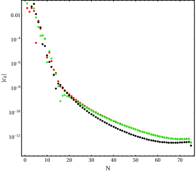
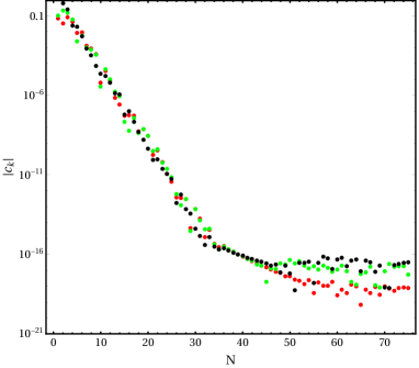
Figure 15: Convergence in the momentum diffusion sector without (left) and with (right) the coordinate mapping $\varrho\mapsto\varrho^{2}$. The $c_{k}$ are the Chebychev coefficients of the numerical solution and $N$ is the number of gridpoints of the Chebychev grid used to discretize the radial direction. The parameters are $\gamma=2/\sqrt{3},\,\tilde{B}=109.658,\,\tilde{\mu}=7.5$ and the fluctuations are $h_{tx},\,h_{zx},\,a_{x}$ (red, green, black).

In section 3.3 we have mentioned a fit of our numerical data for $c_{10}$ and $\tilde{\eta}_{||}$ to the form given in eq. (139). The fit is visualized here in figure 16.

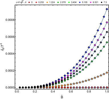
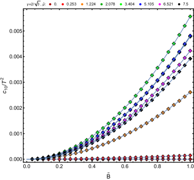
Figure 16: Fit of our numerical data (dots) for $c_{10}$ and $\tilde{\eta}_{||}$ to the form given in eq. (139) (solid lines).

B.4 Computing thermodynamic derivatives of dimensionless quantities

We compute dimensionless quantities of the (conformal) field theory using holography. In particular, we use appropriate powers of the temperature $T$ to introduce the dimensionless chemical potential $\tilde{\mu}=\mu/T$ and the dimensionless magnetic field $\tilde{B}=B/T^{2}.$ In general, for a (thermodynamic) quantity $\mathcal{O}$ with energy dimension $\alpha$ we may introduce the dimensionless quantity $\tilde{\mathcal{O}}=\mathcal{O}/T^{\alpha}.$ Assuming $\mathcal{O}$ is only a function of $(T,\mu,B)$, the dimensionless quantity $\tilde{\mathcal{O}}$ can only depend on the dimensionless quantities, i.e. $(\tilde{\mu},\tilde{B})$. In particular this implies

$$d\mathcal{O}(T,\mu,B)=\left(\frac{\partial\mathcal{O}}{\partial T}\right)_{\mu,B}dT+\left(\frac{\partial\mathcal{O}}{\partial\mu}\right)_{T,B}d\mu+\left(\frac{\partial\mathcal{O}}{\partial B}\right)_{T,\mu}dB\,,$$ (171)

as well as

$$d\mathcal{O}(T,\mu,B)=d\left(T^{\alpha}\,\tilde{\mathcal{O}}(\tilde{\mu},\tilde{B})\right)=\alpha T^{\alpha-1}\tilde{\mathcal{O}}(\tilde{\mu},\tilde{B})\,dT+T^{\alpha}d\tilde{\mathcal{O}}(\tilde{\mu},\tilde{B})\,,$$ (172)

with

$$d\tilde{\mathcal{O}}(\tilde{\mu},\tilde{B})=\left(\frac{\partial\tilde{\mathcal{O}}}{\partial\tilde{\mu}}\right)_{\tilde{B}}d\tilde{\mu}+\left(\frac{\partial\tilde{\mathcal{O}}}{\partial\tilde{B}}\right)_{\tilde{\mu}}d\tilde{B}\,.$$ (173)

Equating both expressions for $d\mathcal{O}$ and using $d\tilde{\mu}=d\mu/T-\mu\,dT/T^{2}$ as well as $d\tilde{B}=dB/T^{2}-2B\,dT/T^{3}$, we may relate derivatives of $\mathcal{O}$ with respect to $T$, $\mu$ and $B$ to derivatives of $\tilde{\mathcal{O}}$ with respect to $\tilde{\mu}$ and $\tilde{B}$ as follows

$$\left(\frac{\partial\mathcal{O}}{\partial\mu}\right)_{T,B} = T^{\alpha-1}\left(\frac{\partial\tilde{\mathcal{O}}}{\partial\tilde{\mu}}\right)_{\tilde{B}}\,,$$ (174)

$$\left(\frac{\partial\mathcal{O}}{\partial B}\right)_{T,\mu} = T^{\alpha-2}\left(\frac{\partial\tilde{\mathcal{O}}}{\partial\tilde{B}}\right)_{\tilde{\mu}}\,,$$ (175)

$$\left(\frac{\partial\mathcal{O}}{\partial T}\right)_{\mu,B} = T^{\alpha-1}\left(-\tilde{\mu}\,\left(\frac{\partial\tilde{\mathcal{O}}}{\partial\tilde{\mu}}\right)_{\tilde{B}}-2\tilde{B}\,\left(\frac{\partial\tilde{\mathcal{O}}}{\partial\tilde{B}}\right)_{\tilde{\mu}}+\alpha\,\tilde{\mathcal{O}}\right)\,.$$ (176)

We may apply those expressions to the case of a grand canonical potential, i.e. $\mathcal{O}(T,\mu,B)=\Omega(T,\mu,B)$ which for a four-dimensional relativistic field theory has energy dimension four, i.e. $\alpha=4$. In this case we obtain the usual relations for the charge density $\rho=-\left(\frac{\partial\Omega}{\partial\mu}\right)_{T,B}$, the magnetization $M=-\left(\frac{\partial\Omega}{\partial B}\right)_{T,\mu}$ and the entropy density $s=-\left(\frac{\partial\Omega}{\partial T}\right)_{\mu,B}$ in terms of their dimensionless counterparts.

References

- (1) A. Cortijo, Y. Ferreirós, K. Landsteiner and M. A. Vozmediano, Elastic gauge fields in weyl semimetals, Physical Review Letters 115 (Oct, 2015).
- (2) D. Pikulin, A. Chen and M. Franz, Chiral anomaly from strain-induced gauge fields in dirac and weyl semimetals, Physical Review X 6 (Oct, 2016).
- (3) A. G. Grushin, J. W. Venderbos, A. Vishwanath and R. Ilan, Inhomogeneous weyl and dirac semimetals: Transport in axial magnetic fields and fermi arc surface states from pseudo-landau levels, Physical Review X 6 (Dec, 2016).
- (4) A. Cortijo, D. Kharzeev, K. Landsteiner and M. A. H. Vozmediano, Strain induced Chiral Magnetic Effect in Weyl semimetals, Phys. Rev. B 94 (2016), no. 24 241405 [1607.03491].
- (5) J. Hernandez and P. Kovtun, Relativistic magnetohydrodynamics, JHEP 05 (2017) 001 [1703.08757].
- (6) D. T. Son and P. Surowka, Hydrodynamics with Triangle Anomalies, Phys. Rev. Lett. 103 (2009) 191601 [0906.5044].
- (7) Y. Neiman and Y. Oz, Relativistic Hydrodynamics with General Anomalous Charges, JHEP 1103 (2011) 023 [1011.5107].
- (8) D. Kharzeev, Parity violation in hot QCD: Why it can happen, and how to look for it, Phys.Lett. B633 (2006) 260–264 [hep-ph/0406125].
- (9) K. Jensen, P. Kovtun and A. Ritz, Chiral conductivities and effective field theory, JHEP 10 (2013) 186 [1307.3234].
- (10) P. Kovtun, Thermodynamics of polarized relativistic matter, JHEP 07 (2016) 028 [1606.01226].
- (11) J. M. Maldacena, The Large N limit of superconformal field theories and supergravity, Int. J. Theor. Phys. 38 (1999) 1113–1133 [hep-th/9711200]. [Adv. Theor. Math. Phys.2,231(1998)].
- (12) E. D’Hoker and P. Kraus, Charged Magnetic Brane Solutions in AdS (5) and the fate of the third law of thermodynamics, JHEP 1003 (2010) 095 [0911.4518].
- (13) A. Vilenkin, Parity Nonconservation and Rotating Black Holes, Phys.Rev.Lett. 41 (1978) 1575–1577.
- (14) A. Vilenkin, Macroscopic parity-violating effects: Neutrino fluxes from rotating black holes and in rotating thermal radiation, Phys. Rev. D 20 (Oct, 1979) 1807–1812.
- (15) A. Vilenkin, Quantum field theory at finite temperature in a rotating system, Phys. Rev. D 21 (1980) 2260–2269.
- (16) J. Erdmenger, M. Haack, M. Kaminski and A. Yarom, Fluid dynamics of R-charged black holes, JHEP 01 (2009) 055 [0809.2488].
- (17) N. Banerjee et. al., Hydrodynamics from charged black branes, JHEP 01 (2011) 094 [0809.2596].
- (18) M. Torabian and H.-U. Yee, Holographic nonlinear hydrodynamics from AdS/CFT with multiple/non-Abelian symmetries, JHEP 08 (2009) 020 [0903.4894].
- (19) D. E. Kharzeev and H. J. Warringa, Chiral Magnetic conductivity, Phys. Rev. D 80 (2009) 034028 [0907.5007].
- (20) D. E. Kharzeev and H.-U. Yee, Chiral Magnetic Wave, Phys. Rev. D83 (2011) 085007 [1012.6026].
- (21) D. E. Kharzeev, The Chiral Magnetic Effect and Anomaly-Induced Transport, Prog. Part. Nucl. Phys. 75 (2014) 133–151 [1312.3348].
- (22) K. Jensen, R. Loganayagam and A. Yarom, Thermodynamics, gravitational anomalies and cones, JHEP 02 (2013) 088 [1207.5824].
- (23) K. Jensen, R. Loganayagam and A. Yarom, Anomaly inflow and thermal equilibrium, JHEP 05 (2014) 134 [1310.7024].
- (24) K. Jensen, M. Kaminski, P. Kovtun, R. Meyer, A. Ritz et. al., Towards hydrodynamics without an entropy current, Phys.Rev.Lett. 109 (2012) 101601 [1203.3556].
- (25) N. Banerjee, J. Bhattacharya, S. Bhattacharyya, S. Jain, S. Minwalla and T. Sharma, Constraints on Fluid Dynamics from Equilibrium Partition Functions, JHEP 09 (2012) 046 [1203.3544].
- (26) S. Bhattacharyya, S. Jain, S. Minwalla and T. Sharma, Constraints on Superfluid Hydrodynamics from Equilibrium Partition Functions, JHEP 01 (2013) 040 [1206.6106].
- (27) J. Bhattacharya, S. Bhattacharyya and M. Rangamani, Non-dissipative hydrodynamics: Effective actions versus entropy current, JHEP 02 (2013) 153 [1211.1020].
- (28) S. Bhattacharyya, J. R. David and S. Thakur, Second order transport from anomalies, JHEP 01 (2014) 010 [1305.0340].
- (29) P. Kovtun and A. Shukla, Kubo formulas for thermodynamic transport coefficients, 1806.05774.
- (30) J. Armas and A. Jain, One-form superfluids \& magnetohydrodynamics, JHEP 01 (2020) 041 [1811.04913].
- (31) P. Kovtun and A. Shukla, Einstein’s equations in matter, Phys. Rev. D 101 (2020), no. 10 104051 [1907.04976].
- (32) S. Grozdanov, D. M. Hofman and N. Iqbal, Generalized global symmetries and dissipative magnetohydrodynamics, Phys. Rev. D 95 (2017), no. 9 096003 [1610.07392].
- (33) F. M. Haehl, R. Loganayagam and M. Rangamani, Effective actions for anomalous hydrodynamics, JHEP 03 (2014) 034 [1312.0610].
- (34) M. Ammon, M. Kaminski, R. Koirala, J. Leiber and J. Wu, Quasinormal modes of charged magnetic black branes & chiral magnetic transport, JHEP 04 (2017) 067 [1701.05565].
- (35) T. Kalaydzhyan and E. Murchikova, Thermal chiral vortical and magnetic waves: new excitation modes in chiral fluids, 1609.00024.
- (36) N. Abbasi, D. Allahbakhshi, A. Davody and S. F. Taghavi, Collective Excitations in QCD Plasma, 1612.08614.
- (37) M. Martinez and M. Strickland, Dissipative Dynamics of Highly Anisotropic Systems, Nucl. Phys. A 848 (2010) 183–197 [1007.0889].
- (38) M. Martinez and M. Strickland, Non-boost-invariant anisotropic dynamics, Nucl. Phys. A 856 (2011) 68–87 [1011.3056].
- (39) R. Ryblewski and W. Florkowski, Non-boost-invariant motion of dissipative and highly anisotropic fluid, J. Phys. G 38 (2011) 015104 [1007.4662].
- (40) R. Ryblewski and W. Florkowski, Highly-anisotropic and strongly-dissipative hydrodynamics with transverse expansion, Eur. Phys. J. C 71 (2011) 1761 [1103.1260].
- (41) R. Ryblewski and W. Florkowski, Highly-anisotropic hydrodynamics in 3+1 space-time dimensions, Phys. Rev. C 85 (2012) 064901 [1204.2624].
- (42) W. Florkowski, M. Martinez, R. Ryblewski and M. Strickland, Anisotropic hydrodynamics - basic concepts, PoS ConfinementX (2012) 221 [1301.7539].
- (43) M. Strickland, Anisotropic Hydrodynamics: Three lectures, Acta Phys. Polon. B 45 (2014), no. 12 2355–2394 [1410.5786].
- (44) X.-G. Huang, A. Sedrakian and D. H. Rischke, Kubo formulae for relativistic fluids in strong magnetic fields, Annals Phys. 326 (2011) 3075–3094 [1108.0602].
- (45) G. Newman, Anomalous hydrodynamics, JHEP 01 (2006) 158 [hep-ph/0511236].
- (46) D. E. Kharzeev, L. D. McLerran and H. J. Warringa, The Effects of topological charge change in heavy ion collisions: ’Event by event P and CP violation’, Nucl.Phys. A803 (2008) 227–253 [0711.0950].
- (47) K. Fukushima, D. E. Kharzeev and H. J. Warringa, The Chiral Magnetic Effect, Phys. Rev. D78 (2008) 074033 [0808.3382].
- (48) U. Gursoy and J. Tarrio, Horizon universality and anomalous conductivities, JHEP 10 (2015) 058 [1410.1306].
- (49) S. Grozdanov and N. Poovuttikul, Universality of anomalous conductivities in theories with higher-derivative holographic duals, JHEP 09 (2016) 046 [1603.08770].
- (50) U. Gürsoy and A. Jansen, (Non)renormalization of Anomalous Conductivities and Holography, JHEP 10 (2014) 092 [1407.3282].
- (51) A. Jimenez-Alba, K. Landsteiner and L. Melgar, Anomalous magnetoresponse and the Stückelberg axion in holography, Phys. Rev. D90 (2014) 126004 [1407.8162].
- (52) A. D. Gallegos and U. Gursoy, Dynamical gauge fields and anomalous transport at strong coupling, 1806.07138.
- (53) S. Golkar and D. T. Son, (Non)-renormalization of the chiral vortical effect coefficient, JHEP 02 (2015) 169 [1207.5806].
- (54) I. Amado, K. Landsteiner and F. Pena-Benitez, Anomalous transport coefficients from Kubo formulas in Holography, JHEP 1105 (2011) 081 [1102.4577].
- (55) K. Landsteiner, E. Megias and F. Pena-Benitez, Frequency dependence of the Chiral Vortical Effect, Phys. Rev. D90 (2014), no. 6 065026 [1312.1204].
- (56) S. Li and H.-U. Yee, Relaxation Times for Chiral Transport Phenomena and Spin Polarization in Strongly Coupled Plasma, 1805.04057.
- (57) Y. Matsuo, S.-J. Sin, S. Takeuchi and T. Tsukioka, Magnetic conductivity and Chern-Simons Term in Holographic Hydrodynamics of Charged AdS Black Hole, JHEP 04 (2010) 071 [0910.3722].
- (58) S. Grozdanov and N. Poovuttikul, Generalised global symmetries in holography: magnetohydrodynamic waves in a strongly interacting plasma, JHEP 04 (2019) 141 [1707.04182].
- (59) R. Critelli, S. I. Finazzo, M. Zaniboni and J. Noronha, Anisotropic shear viscosity of a strongly coupled non-Abelian plasma from magnetic branes, Phys. Rev. D90 (2014), no. 6 066006 [1406.6019].
- (60) S. I. Finazzo, R. Critelli, R. Rougemont and J. Noronha, Erratum: Momentum transport in strongly coupled anisotropic plasmas in the presence of strong magnetic fields [phys. rev. d 94, 054020 (2016)], Phys. Rev. D 96 (Jul, 2017) 019903.
- (61) M. Ammon, S. Grieninger, A. Jimenez-Alba, R. P. Macedo and L. Melgar, Holographic quenches and anomalous transport, JHEP 09 (2016) 131 [1607.06817].
- (62) S. Janiszewski and M. Kaminski, Quasinormal modes of magnetic and electric black branes versus far from equilibrium anisotropic fluids, Phys. Rev. D93 (2016), no. 2 025006 [1508.06993].
- (63) M. Baggioli, S. Grieninger and L. Li, Magnetophonons & type-B Goldstones from Hydrodynamics to Holography, JHEP 09 (2020) 037 [2005.01725].
- (64) A. Rebhan, A. Schmitt and S. A. Stricker, Anomalies and the chiral magnetic effect in the Sakai-Sugimoto model, JHEP 1001 (2010) 026 [0909.4782].
- (65) J. Erdmenger, P. Kerner and H. Zeller, Non-universal shear viscosity from Einstein gravity, Phys. Lett. B 699 (2011) 301–304 [1011.5912].
- (66) J. Erdmenger, M. Rangamani, S. Steinfurt and H. Zeller, Hydrodynamic Regimes of Spinning Black D3-Branes, JHEP 02 (2015) 026 [1412.0020].
- (67) M. Garbiso and M. Kaminski, Hydrodynamics of simply spinning black holes & hydrodynamics for spinning quantum fluids, 2007.04345.
- (68) J.-W. Chen, S. Pu, Q. Wang and X.-N. Wang, Berry Curvature and Four-Dimensional Monopoles in the Relativistic Chiral Kinetic Equation, Phys. Rev. Lett. 110 (2013), no. 26 262301 [1210.8312].
- (69) K. Landsteiner, E. Megias and F. Pena-Benitez, Gravitational Anomaly and Transport, Phys.Rev.Lett. 107 (2011) 021601 [1103.5006].
- (70) M. Stone and J. Kim, Mixed Anomalies: Chiral Vortical Effect and the Sommerfeld Expansion, Phys. Rev. D 98 (2018), no. 2 025012 [1804.08668].
- (71) K. Landsteiner, E. Megias, L. Melgar and F. Pena-Benitez, Holographic Gravitational Anomaly and Chiral Vortical Effect, JHEP 09 (2011) 121 [1107.0368].
- (72) K. Landsteiner, Notes on Anomaly Induced Transport, Acta Phys. Polon. B47 (2016) 2617 [1610.04413].
- (73) C. G. Callan, Jr. and J. A. Harvey, Anomalies and Fermion Zero Modes on Strings and Domain Walls, Nucl. Phys. B250 (1985) 427–436.
- (74) R. Loganayagam, Anomaly Induced Transport in Arbitrary Dimensions, 1106.0277.
- (75) F. M. Haehl, R. Loganayagam and M. Rangamani, Effective Action for Relativistic Hydrodynamics: Fluctuations, Dissipation, and Entropy Inflow, JHEP 10 (2018) 194 [1803.11155].
- (76) H. Liu and P. Glorioso, Lectures on non-equilibrium effective field theories and fluctuating hydrodynamics, PoS TASI2017 (2018) 008 [1805.09331].
- (77) K. Jensen, R. Marjieh, N. Pinzani-Fokeeva and A. Yarom, A panoply of Schwinger-Keldysh transport, SciPost Phys. 5 (2018), no. 5 053 [1804.04654].
- (78) P. Kovtun, G. D. Moore and P. Romatschke, The stickiness of sound: An absolute lower limit on viscosity and the breakdown of second order relativistic hydrodynamics, Phys.Rev. D84 (2011) 025006 [1104.1586].
- (79) P. Kovtun, First-order relativistic hydrodynamics is stable, JHEP 10 (2019) 034 [1907.08191].
- (80) R. E. Hoult and P. Kovtun, Stable and causal relativistic Navier-Stokes equations, JHEP 06 (2020) 067 [2004.04102].
- (81) F. S. Bemfica, M. M. Disconzi and J. Noronha, Causality and existence of solutions of relativistic viscous fluid dynamics with gravity, Phys. Rev. D 98 (2018), no. 10 104064 [1708.06255].
- (82) F. S. Bemfica, M. M. Disconzi and J. Noronha, Nonlinear Causality of General First-Order Relativistic Viscous Hydrodynamics, Phys. Rev. D 100 (2019), no. 10 104020 [1907.12695].
- (83) F. S. Bemfica, M. M. Disconzi and J. Noronha, General-Relativistic Viscous Fluid Dynamics, 2009.11388.
- (84) L. Onsager, Reciprocal relations in irreversible processes. i., Phys. Rev. 37 (Feb, 1931) 405–426.
- (85) L. Onsager, Reciprocal relations in irreversible processes. ii., Phys. Rev. 38 (Dec, 1931) 2265–2279.
- (86) S. Bhattacharyya, Entropy current and equilibrium partition function in fluid dynamics, JHEP 08 (2014) 165 [1312.0220].
- (87) S. Bhattacharyya, Entropy Current from Partition Function: One Example, JHEP 07 (2014) 139 [1403.7639].
- (88) K. Jensen, M. Kaminski, P. Kovtun, R. Meyer, A. Ritz et. al., Parity-Violating Hydrodynamics in 2+1 Dimensions, JHEP 1205 (2012) 102 [1112.4498].
- (89) S. A. Hartnoll, P. K. Kovtun, M. Muller and S. Sachdev, Theory of the Nernst effect near quantum phase transitions in condensed matter, and in dyonic black holes, Phys.Rev. B76 (2007) 144502 [0706.3215].
- (90) J. E. Avron, R. Seiler and P. G. Zograf, Viscosity of quantum Hall fluids, Phys. Rev. Lett. 75 (1995) 697–700 [cond-mat/9502011].
- (91) J. E. Avron, Odd Viscosity, arXiv e-prints (Dec., 1997) physics/9712050 [physics/9712050].
- (92) M. Chernodub, A. Cortijo and M. A. Vozmediano, Generation of a Nernst Current from the Conformal Anomaly in Dirac and Weyl Semimetals, Phys. Rev. Lett. 120 (2018), no. 20 206601 [1712.05386].
- (93) F. Haldane, Model for a Quantum Hall Effect without Landau Levels: Condensed-Matter Realization of the ’Parity Anomaly’, Phys.Rev.Lett. 61 (1988) 2015–2018.
- (94) J. Hernandez, Exploring the fluid landscape: three new regimes of relativistic hydrodynamics, Master’s thesis, U. Victoria (main), 2017. https://dspace.library.uvic.ca/bitstream/handle/1828/8449/Hernandez_Juan_MSc_2017.pdf.
- (95) M. Ammon and J. Erdmenger, Gauge/gravity duality. Cambridge Univ. Pr., Cambridge, UK, 2015.
- (96) H. Nastase, Introduction to the AdS/CFT Correspondence. Cambridge Univ. Pr., Cambridge, UK, 2015.
- (97) J. Zaanen, Y. Liu, Y.-W. Sun and K. Schalm, Holographic Duality in Condensed Matter Physics. Cambridge Univ. Pr., Cambridge, UK, 2016.
- (98) E. D’Hoker and P. Kraus, Magnetic Brane Solutions in AdS, JHEP 0910 (2009) 088 [0908.3875].
- (99) M. Ammon, J. Leiber and R. P. Macedo, Phase diagram of 4D field theories with chiral anomaly from holography, JHEP 03 (2016) 164 [1601.02125].
- (100) M. Ammon, J. Erdmenger, P. Kerner and M. Strydom, Black Hole Instability Induced by a Magnetic Field, Phys. Lett. B 706 (2011) 94–99 [1106.4551].
- (101) A. Buchel and J. T. Liu, Gauged supergravity from type IIB string theory on Y**p,q manifolds, Nucl. Phys. B771 (2007) 93–112 [hep-th/0608002].
- (102) J. P. Gauntlett, E. O Colgain and O. Varela, Properties of some conformal field theories with M-theory duals, JHEP 02 (2007) 049 [hep-th/0611219].
- (103) J. P. Gauntlett and O. Varela, Consistent Kaluza-Klein reductions for general supersymmetric AdS solutions, Phys. Rev. D76 (2007) 126007 [0707.2315].
- (104) E. O. Colgáin, M. M. Sheikh-Jabbari, J. F. Vázquez-Poritz, H. Yavartanoo and Z. Zhang, Warped Ricci-flat reductions, Phys. Rev. D90 (2014), no. 4 045013 [1406.6354].
- (105) M. Henningson and K. Skenderis, The Holographic Weyl anomaly, JHEP 07 (1998) 023 [hep-th/9806087].
- (106) V. Balasubramanian and P. Kraus, A Stress tensor for Anti-de Sitter gravity, Commun.Math.Phys. 208 (1999) 413–428 [hep-th/9902121].
- (107) M. Taylor, More on counterterms in the gravitational action and anomalies, hep-th/0002125.
- (108) B. Sahoo and H.-U. Yee, Electrified plasma in AdS/CFT correspondence, JHEP 11 (2010) 095 [1004.3541].
- (109) C. Fefferman and C. R. Graham, Conformal invariants, in The Mathematical Heritage of Élie Cartan (Lyon, 1984), Astérisque, Numero Hors Serie (1985) 95–116.
- (110) C. Fefferman and C. R. Graham, The ambient metric, Ann. Math. Stud. 178 (2011) 1–128 [0710.0919].
- (111) E. Alvarez, J. Conde and L. Hernandez, A Note on the Bach tensor in AdS / CFT, hep-th/0206140.
- (112) A. Gynther, K. Landsteiner, F. Pena-Benitez and A. Rebhan, Holographic Anomalous Conductivities and the Chiral Magnetic Effect, JHEP 02 (2011) 110 [1005.2587].
- (113) K. Landsteiner, E. Megias, L. Melgar and F. Pena-Benitez, Gravitational Anomaly and Hydrodynamics, J. Phys. Conf. Ser. 343 (2012) 012073 [1111.2823].
- (114) J. F. Fuini and L. G. Yaffe, Far-from-equilibrium dynamics of a strongly coupled non-Abelian plasma with non-zero charge density or external magnetic field, JHEP 07 (2015) 116 [1503.07148].
- (115) M. Ammon, V. G. Filev, J. Tarrio and D. Zoakos, D3/D7 Quark-Gluon Plasma with Magnetically Induced Anisotropy, JHEP 09 (2012) 039 [1207.1047].
- (116) Y. Bu and S. Lin, Magneto-vortical effect in strongly coupled plasma, Eur. Phys. J. C 80 (2020), no. 5 401 [1912.11277].
- (117) A. Jimenez-Alba and L. Melgar, Anomalous Transport in Holographic Chiral Superfluids via Kubo Formulae, JHEP 10 (2014) 120 [1404.2434].
- (118) K. Landsteiner and Y. Liu, The holographic Weyl semi-metal, Phys. Lett. B753 (2016) 453–457 [1505.04772].
- (119) K. Landsteiner, Y. Liu and Y.-W. Sun, Quantum phase transition between a topological and a trivial semimetal from holography, Phys. Rev. Lett. 116 (2016), no. 8 081602 [1511.05505].
- (120) C. Copetti, J. Fernandez-Pendas and K. Landsteiner, Axial Hall effect and universality of holographic Weyl semi-metals, 1611.08125.
- (121) M. Ammon, M. Heinrich, A. Jimenez-Alba and S. Moeckel, Surface States in Holographic Weyl Semimetals, 1612.00836.
- (122) G. Grignani, A. Marini, F. Pena-Benitez and S. Speziali, AC conductivity for a holographic Weyl Semimetal, 1612.00486.
- (123) STAR Collaboration, L. Adamczyk et. al., Global hyperon polarization in nuclear collisions: evidence for the most vortical fluid, Nature 548 (2017) 62–65 [1701.06657].
- (124) V. E. Ambrus and M. Chernodub, Helical vortical effects, helical waves, and anomalies of Dirac fermions, 1912.11034.
- (125) V. E. Ambrus and M. Chernodub, Hyperon–anti-hyperon polarization asymmetry in relativistic heavy-ion collisions as an interplay between chiral and helical vortical effects, 2010.05831.
- (126) A. Boyarsky, J. Frohlich and O. Ruchayskiy, Magnetohydrodynamics of Chiral Relativistic Fluids, Phys. Rev. D 92 (2015) 043004 [1504.04854].
- (127) M. Crossley, P. Glorioso and H. Liu, Effective field theory of dissipative fluids, JHEP 09 (2017) 095 [1511.03646].
- (128) F. M. Haehl, R. Loganayagam and M. Rangamani, Adiabatic hydrodynamics: The eightfold way to dissipation, JHEP 05 (2015) 060 [1502.00636].
- (129) F. M. Haehl, R. Loganayagam and M. Rangamani, The Fluid Manifesto: Emergent symmetries, hydrodynamics, and black holes, JHEP 01 (2016) 184 [1510.02494].
- (130) F. M. Haehl, R. Loganayagam and M. Rangamani, Schwinger-Keldysh formalism. Part I: BRST symmetries and superspace, JHEP 06 (2017) 069 [1610.01940].
- (131) C. Hoyos, S. Moroz and D. Thanh Son, Effective theory of chiral two-dimensional superfluids, 1305.3925.
- (132) P. Romatschke, Relativistic Fluid Dynamics Far From Local Equilibrium, Phys. Rev. Lett. 120 (2018), no. 1 012301 [1704.08699].
- (133) M. P. Heller, D. Mateos, W. van der Schee and M. Triana, Holographic isotropization linearized, JHEP 09 (2013) 026 [1304.5172].
- (134) M. P. Heller and M. Spalinski, Hydrodynamics Beyond the Gradient Expansion: Resurgence and Resummation, Phys. Rev. Lett. 115 (2015), no. 7 072501 [1503.07514].
- (135) M. P. Heller, R. Jefferson, M. Spaliński and V. Svensson, Hydrodynamic attractors in phase space, Phys. Rev. Lett. 125 (2020), no. 13 132301 [2003.07368].
- (136) M. P. Heller, A. Serantes, M. Spaliński, V. Svensson and B. Withers, The hydrodynamic gradient expansion in linear response theory, 2007.05524.
- (137) Y. Bu, M. Lublinsky and A. Sharon, Anomalous transport from holography: Part I, JHEP 11 (2016) 093 [1608.08595].
- (138) Y. Bu, M. Lublinsky and A. Sharon, Anomalous transport from holography: Part II, 1609.09054.
- (139) Y. Bu, T. Demircik and M. Lublinsky, Gradient resummation for nonlinear chiral transport: an insight from holography, Eur. Phys. J. C 79 (2019), no. 1 54 [1807.11908].
- (140) Y. Bu, T. Demircik and M. Lublinsky, Nonlinear chiral transport from holography, JHEP 01 (2019) 078 [1807.08467].
- (141) Y. Bu, T. Demircik and M. Lublinsky, Chiral transport in strong fields from holography, 1903.00896.
- (142) P. Romatschke and U. Romatschke, Relativistic Fluid Dynamics In and Out of Equilibrium. Cambridge Monographs on Mathematical Physics. Cambridge University Press, 5, 2019.
- (143) J. M. Stewart, Relativistic Hydrodynamics, by Luciano Rezzolla and Olindo Zanotti. Scope: monograph, text book. Level: postgraduate, advanced undergraduate, early career researcher, researcher, Contemporary Physics 55 (Oct., 2014) 354–355.
- (144) M. Joyce and M. E. Shaposhnikov, Primordial magnetic fields, right-handed electrons, and the Abelian anomaly, Phys. Rev. Lett. 79 (1997) 1193–1196 [astro-ph/9703005].
- (145) A. Boyarsky, J. Frohlich and O. Ruchayskiy, Self-consistent evolution of magnetic fields and chiral asymmetry in the early Universe, Phys. Rev. Lett. 108 (2012) 031301 [1109.3350].
- (146) H. Tashiro, T. Vachaspati and A. Vilenkin, Chiral Effects and Cosmic Magnetic Fields, Phys. Rev. D 86 (2012) 105033 [1206.5549].
- (147) A. Brandenburg, J. Schober, I. Rogachevskii, T. Kahniashvili, A. Boyarsky, J. Frohlich, O. Ruchayskiy and N. Kleeorin, The turbulent chiral-magnetic cascade in the early universe, Astrophys. J. Lett. 845 (2017), no. 2 L21 [1707.03385].
- (148) A. Boyarsky, V. Cheianov, O. Ruchayskiy and O. Sobol, Equilibration of the chiral asymmetry due to finite electron mass in electron-positron plasma, 2008.00360.
- (149) A. Boyarsky, V. Cheianov, O. Ruchayskiy and O. Sobol, Evolution of the primordial axial charge across cosmic times, 2007.13691.
- (150) M. Fujita, M. Kaminski and A. Karch, SL(2,Z) Action on AdS/BCFT and Hall Conductivities, JHEP 07 (2012) 150 [1204.0012].
- (151) Y.-S. An, T. Ji and L. Li, Magnetotransport and Complexity of Holographic Metal-Insulator Transitions, JHEP 10 (2020) 023 [2007.13918].
- (152) C. Hoyos, R. Lier, F. Peña Benitez and P. Surówka, Quantum Hall effective action for the anisotropic Dirac semimetal, Phys. Rev. B 102 (2020), no. 8 081303 [2006.14595].
- (153) M. N. Chernodub, A. Cortijo, A. G. Grushin, K. Landsteiner and M. A. H. Vozmediano, Condensed matter realization of the axial magnetic effect, Phys. Rev. B 89 (2014), no. 8 081407 [1311.0878].
- (154) P. Buividovich, M. Chernodub, E. Luschevskaya and M. Polikarpov, Numerical evidence of chiral magnetic effect in lattice gauge theory, Phys. Rev. D 80 (2009) 054503 [0907.0494].
- (155) P. Buividovich, M. Chernodub, D. Kharzeev, T. Kalaydzhyan, E. Luschevskaya and M. Polikarpov, Magnetic-Field-Induced insulator-conductor transition in SU(2) quenched lattice gauge theory, Phys. Rev. Lett. 105 (2010) 132001 [1003.2180].
- (156) G. Bali, F. Bruckmann, G. Endrodi, Z. Fodor, S. Katz, S. Krieg, A. Schafer and K. Szabo, The QCD phase diagram for external magnetic fields, JHEP 02 (2012) 044 [1111.4956].
- (157) G. Bali, F. Bruckmann, G. Endrodi, Z. Fodor, S. Katz and A. Schafer, QCD quark condensate in external magnetic fields, Phys. Rev. D 86 (2012) 071502 [1206.4205].
- (158) G. Bali, F. Bruckmann, G. Endrödi, S. Katz and A. Schäfer, The QCD equation of state in background magnetic fields, JHEP 08 (2014) 177 [1406.0269].
- (159) N. Yu. Astrakhantsev, V. V. Braguta, M. D’Elia, A. Yu. Kotov, A. A. Nikolaev and F. Sanfilippo, Lattice study of electromagnetic conductivity of quark-gluon plasma in external magnetic field, 1910.08516.
- (160) G. Endrodi, M. Kaminski, A. Schafer, J. Wu and L. Yaffe, Universal Magnetoresponse in QCD and SYM, JHEP 09 (2018) 070 [1806.09632].
- (161) V. Voronyuk, V. Toneev, W. Cassing, E. Bratkovskaya, V. Konchakovski and S. Voloshin, (Electro-)Magnetic field evolution in relativistic heavy-ion collisions, Phys. Rev. C 83 (2011) 054911 [1103.4239].
- (162) G. Inghirami, M. Mace, Y. Hirono, L. Del Zanna, D. E. Kharzeev and M. Bleicher, Magnetic fields in heavy ion collisions: flow and charge transport, Eur. Phys. J. C 80 (2020), no. 3 293 [1908.07605].
- (163) X.-G. Wen, Colloquium: Zoo of quantum-topological phases of matter, Reviews of Modern Physics 89 (Oct., 2017) 041004 [1610.03911].
- (164) C. Hoyos, Hall viscosity, topological states and effective theories, Int. J. Mod. Phys. B 28 (2014) 1430007 [1403.4739].
- (165) N. Read, Non-Abelian adiabatic statistics and Hall viscosity in quantum Hall states and p(x) + ip(y) paired superfluids, Phys. Rev. B 79 (2009) 045308 [0805.2507].
- (166) N. Read and E. Rezayi, Hall viscosity, orbital spin, and geometry: paired superfluids and quantum Hall systems, Phys. Rev. B 84 (2011) 085316 [1008.0210].
- (167) D. T. Son and C. Wu, Holographic Spontaneous Parity Breaking and Emergent Hall Viscosity and Angular Momentum, JHEP 07 (2014) 076 [1311.4882].
- (168) N. Nagaosa, J. Sinova, S. Onoda, A. H. MacDonald and N. P. Ong, Anomalous Hall effect, Reviews of Modern Physics 82 (Apr., 2010) 1539–1592 [0904.4154].
- (169) H. Nielsen and M. Ninomiya, The adler-bell-jackiw anomaly and weyl fermions in a crystal, Physics Letters B 130 (1983), no. 6 389 – 396.
- (170) D. I. Pikulin, A. Chen and M. Franz, Chiral anomaly from strain-induced gauge fields in dirac and weyl semimetals, Phys. Rev. X 6 (Oct, 2016) 041021.
- (171) K. Taguchi, T. Imaeda, M. Sato and Y. Tanaka, Photovoltaic chiral magnetic effect in weyl semimetals, Phys. Rev. B 93 (May, 2016) 201202.
- (172) D. Breunig, S.-B. Zhang, M. Stehno and B. Trauzettel, Influence of a chiral chemical potential on Weyl hybrid junctions, Phys. Rev. B 99 (2019), no. 17 174501 [1903.06229].
- (173) S.-B. Zhang, F. Dolcini, D. Breunig and B. Trauzettel, Appearance of the universal value of the zero-bias conductance in a weyl semimetal-superconductor junction, Phys. Rev. B 97 (Jan, 2018) 041116.
- (174) Q. Li, D. E. Kharzeev, C. Zhang, Y. Huang, I. Pletikosic, A. V. Fedorov, R. D. Zhong, J. A. Schneeloch, G. D. Gu and T. Valla, Observation of the chiral magnetic effect in ZrTe5, ArXiv e-prints (Dec., 2014) [1412.6543].
- (175) C. Shekhar, F. Arnold, S.-C. Wu, Y. Sun, M. Schmidt, N. Kumar, A. G. Grushin, J. H. Bardarson, R. Donizeth dos Reis, M. Naumann, M. Baenitz, H. Borrmann, M. Nicklas, E. Hassinger, C. Felser and B. Yan, Large and unsaturated negative magnetoresistance induced by the chiral anomaly in the Weyl semimetal TaP, ArXiv e-prints (June, 2015) [1506.06577].
- (176) C. Zhang, E. Zhang, Y. Liu, Z.-G. Chen, S. Liang, J. Cao, X. Yuan, L. Tang, Q. Li, T. Gu, Y. Wu, J. Zou and F. Xiu, Detection of chiral anomaly and valley transport in Dirac semimetals, ArXiv e-prints (Apr., 2015) [1504.07698].
- (177) Z. Wang, Y. Zheng, Z. Shen, Y. Zhou, X. Yang, Y. Li, C. Feng and Z.-A. Xu, Helicity protected ultrahigh mobility Weyl fermions in NbP, ArXiv e-prints (June, 2015) [1506.00924].
- (178) X. Yang, Y. Liu, Z. Wang, Y. Zheng and Z.-a. Xu, Chiral anomaly induced negative magnetoresistance in topological Weyl semimetal NbAs, ArXiv e-prints (June, 2015) [1506.03190].
- (179) A. Baumgartner, A. Karch and A. Lucas, Magnetoresistance in relativistic hydrodynamics without anomalies, JHEP 06 (2017) 054 [1704.01592].
- (180) M. Ammon, T. H. Ngo and A. O’Bannon, Holographic Flavor Transport in Arbitrary Constant Background Fields, JHEP 10 (2009) 027 [0908.2625].
- (181) D. Kharzeev, Y. Kikuchi and R. Meyer, Chiral magnetic effect without chirality source in asymmetric Weyl semimetals, Eur. Phys. J. B 91 (2018), no. 5 83 [1610.08986].
- (182) A. I. Berdyugin, S. G. Xu, F. M. D. Pellegrino, R. Krishna Kumar, A. Principi, I. Torre, M. Ben Shalom, T. Taniguchi, K. Watanabe, I. V. Grigorieva, M. Polini, A. K. Geim and D. A. Bandurin, Measuring hall viscosity of graphene’s electron fluid, Science 364 (2019), no. 6436 162–165 [https://science.sciencemag.org/content/364/6436/162.full.pdf].
- (183) L. W. Molenkamp and M. J. M. de Jong, Electron-electron-scattering-induced size effects in a two-dimensional wire, Phys. Rev. B 49 (Feb, 1994) 5038–5041.
- (184) P. J. W. Moll, P. Kushwaha, N. Nandi, B. Schmidt and A. P. Mackenzie, Evidence for hydrodynamic electron flow in pdcoo2, Science 351 (2016), no. 6277 1061–1064 [https://science.sciencemag.org/content/351/6277/1061.full.pdf].
- (185) D. Di Sante, J. Erdmenger, M. Greiter, I. Matthaiakakis, R. Meyer, D. Rodríguez Fernández, R. Thomale, E. van Loon and T. Wehling, Turbulent hydrodynamics in strongly correlated Kagome metals, Nature Commun. 11 (2020), no. 1 3997 [1911.06810].
- (186) C. Tutschku, F. S. Nogueira, C. Northe, J. van den Brink and E. Hankiewicz, Temperature and chemical potential dependence of the parity anomaly in quantum anomalous Hall insulators, Phys. Rev. B 102 (2020), no. 20 205407 [2007.11852].
- (187) C. Tutschku, J. Böttcher, R. Meyer and E. Hankiewicz, Momentum-Dependent Mass and AC Hall Conductivity of Quantum Anomalous Hall Insulators and Their Relation to the Parity Anomaly, Phys. Rev. Res. 2 (2020), no. 3 033193 [2003.03146].
- (188) J. Böttcher, C. Tutschku, L. W. Molenkamp and E. M. Hankiewicz, Survival of the quantum anomalous hall effect in orbital magnetic fields as a consequence of the parity anomaly, Phys. Rev. Lett. 123 (Nov, 2019) 226602.
- (189) J. P. Boyd, Chebyshev and Fourier Spectral Methods (Second Edition, Revised). Dover Publications, New York, 2001.
- (190) S. Grieninger, Holographic quenches and anomalous transport, 1711.08422.
- (191) S. Grieninger, Non-equilibrium dynamics in Holography. PhD thesis, Jena U., 2020. 2012.10109.
- (192) M. Baggioli and S. Grieninger, Zoology of solid & fluid holography — Goldstone modes and phase relaxation, JHEP 10 (2019) 235 [1905.09488].